Theory of Thermal Conductivity on Excitonic Insulator

Abstract

We study the thermal conductivity in the excitonic insulator using a simple quasi one-dimensional two-band model consisting of electron and hole bands with the Coulomb interactions between these bands. Based on the linear response theory within a mean-field scheme, we develop a method to identify the contributions to thermal conductivity driven by excitonic insulator. It is found that there is an additional heat current operator owing to the excitonic phase transition, and that it gives contributions to thermal conductivity which are not expressed in the form of Sommerfeld-Bethe relations written in the form of an imaginary-time derivative of the electric current operator. Finally, we discuss the relationship between the newly-found additional contribution and the heat current carried by excitons.

I introduction

An excitonic insulator (EI) is one of the interesting correlated phases of narrow-gap semiconductors and semimetals. It was proposed in the 60s that Coulomb interaction between conduction band electrons and valence band holes can lead to a spontaneous formation of excitons, and their condensation induces a nonconducting state mott ; blatt ; knox ; kohn ; jerome ; halperin . Various theoretical studies have been carried out on EI, and one of the most important and interesting aspects of these studies is that the excitonic theory can be transformed to the BCS theory by a particle-hole transformation kohn ; jerome ; halperin . Then, various properties such as anisotropic band structure zittartz4 , impurity effect zittartz1 , transport properties jerome ; zittartz2 ; zittartz3 , and effect of magnetic field fenton have been extensively discussed in terms of similarity or symmetry with the superconducting theory. However, no materials have been identified as EI at that time.

Recently, growing number of promising candidate materials for EI have actually been proposed, raising researchers’ interest to study the EI phase. For example, ${\rm Tm}({\rm Se,Te})$ bucher ; wachter2 , $1T$-${\rm TiSe}_{2}$ wilson ; cercellier , and ${\rm Ta}_{2}{\rm NiSe}_{5}$ tanise1 ; wakisaka ; tanise2 have been proposed on the basis of various transport measurements neuenschwander ; wachter , angle-resolved photoemission spectroscopy (ARPES) cercellier ; tanise1 ; wakisaka , and systematic elemental substitutions zerogap . In particular, after ${\rm Ta}_{2}{\rm NiSe}_{5}$ was proposed, many experiments have been performed on ${\rm Ta}_{2}{\rm NiSe}_{5}$, such as spectroscopic ellipsometry ellipsometry , observation of electron-phonon coupling and exciton-phonon coupling epc1 ; epc2 ; epc3 , transport studies on bulk and thin-film samples thin , and study of electrical tuning of the EI ground state tuning . The EI phase is also being actively studied theoretically, including calculation of the BCS-BEC crossover bronold ; crossover , electron-phonon coupling epc4 , spin-orbit coupling soc , and the topological EI states topological . With that, the verification of the theories and experiments has become increasingly important. It is interesting to note that some theoretical calculations reproduce the ARPES results tanise2 , the superconductivity in the vicinity of the excitonic phase tyoudendou ; tyoudendouriron and peculiar temperature dependence of orbital susceptibility taijiritu ; matsuura .

The proposals of new candidate materials have also been pursued, such as semiconductor materials handoutai ; inas , electron-hole bilayers bilayer , graphene graphen1 ; graphen2 and iron-based superconductors fe ; fe2 . However, in actual materials, the EI phase often coexists with the charge density waves and staggered orbital orders difficulty1 ; difficulty2 , and it is still difficult to determine the EI state by experiments. Considering the verification of experimental and theoretical studies and the creation of new materials, it is important to develop methods other than photoemission spectroscopy to identify EI. Thermal conductivity in EI is also one of the interesting topics. This is because the excitons do not have electronic charges, but have energies contributing to the heat current. Indeed, it was observed that the thermal conductivity of ${\rm TmSe}_{0.45}{\rm Te}_{0.55}$, which is a candidate material of EI, shows unusual temperature dependence wachter .

When the thermal conductivity is written in the form of an imaginary-time derivative of the electric current, as shown by Jonson and Mahan jonson , the following relations hold:

$$L_{11}= \int^{\infty}_{-\infty}d\epsilon\left(-\frac{d\,f\left(\epsilon\right)}{d\epsilon}\right)\sigma\left(\epsilon\right),$$ (1a)

$$L_{21}= \int^{\infty}_{-\infty}d\epsilon\,\frac{\epsilon-\mu}{e}\left(-\frac{d\,f\left(\epsilon\right)}{d\epsilon}\right)\sigma\left(\epsilon\right),$$ (1b)

$$L_{22}= \int^{\infty}_{-\infty}d\epsilon\left(\frac{\epsilon-\mu}{e}\right)^{2}\left(-\frac{d\,f\left(\epsilon\right)}{d\epsilon}\right)\sigma\left(\epsilon\right),$$ (1c)

where the linear response coefficients, $L_{ij}\ \left(i,j=1,2\right)$, are defined by linear

$$\begin{split}\bm{j}&=L_{11}\bm{E}+L_{12}\left(-\frac{\nabla T}{T}\right),\\ \bm{j}^{Q}&=L_{21}\bm{E}+L_{22}\left(-\frac{\nabla T}{T}\right).\end{split}$$ (2)

Here, $\bm{j}$, $\bm{j}^{Q}$, $\bm{E}$, $T$, and $\nabla T$ are electric current density, heat current density, electric field, temperature, and temperature gradient, respectively, and $e$ is electron charge ($e<0$) and $f\left(\epsilon\right)=1/\left(e^{\beta\left(\epsilon-\mu\right)}+1\right)$ is the Fermi distribution function, where $\beta=1/k_{B}T$, and $\mu$ and $k_{B}$ are the chemical potential and Boltzmann constant. Due to Onsager’s reciprocal theorem, $L_{12}=L_{21}$ holds. The electrical conductivity is $L_{11}$, and the thermal conductivity $\kappa$, which is defined as the ratio of $\bm{j}_{Q}$ to $-\nabla T$ under the $\bm{j}=0$ condition, is given by

$$\kappa=\left(L_{22}-L_{21}L_{12}/L_{11}\right)/T.$$ (3)

Since excitons do not carry electrical charge, $L_{11}$ in Eq. (1a) should be due to quasiparticles and not due to excitons. Correspondingly, $L_{21}$ and $L_{22}$ in Eqs. (1b) and (1c) should be also due to quasiparticles. Therefore, if the excitons, when they are condensed below transition temperature, contribute to heat current, then there must be additional contributions to $L_{21}$ and $L_{22}$ that are not expressed as in Eqs. (1b) and (1c). To clarify the discussion in the following, we call Eqs. (1b) and (1c) as Sommerfeld-Bethe (SB) relation for $L_{21}$ fukuyama and SB relation for $L_{22}$, because Eqs. (1b) and (1c) can be obtained from the Boltzmann’s equation sb . In the previous studies zittartz3 ; kurihara , the thermal conductivity was discussed on the basis of Eqs. (1a) $\sim$ (1c). Thus, the exciton contributions were not taken into account.

In this paper, we study the thermal conductivity in a model for EI to identify the additional contribution derived from EI, which is beyond the SB relations. First, we microscopically obtain the heat current operator in a model for EI ohta ; matsuura , or a simple quasi one-dimensional two-band model. Then, we study the linear response theory kubo ; luttinger of $L_{11}$, $L_{21}$, and $L_{22}$ within a mean-field scheme to introduce the order parameters of EI. We will show that, by considering two types of nearest-neighbor interactions, additional heat current operators owing to the EI phase transition exist and give the contributions in $L_{21}$ and $L_{22}$ which are not expressed in the form of Eqs. (1b) and (1c). Finally, we discuss the relationship between this additional contribution and the heat current due to excitons.

Theoretically, the validity of the SB relations, Eqs. (1a) $\sim$ (1c), has been discussed jonson ; kontani ; fukuyama . Jonson and Mahan showed that, in the presence of potential (including random potentials) and the electron-phonon interaction, the SB relations holds, except for a single term in the heat current operator which is due to the electron-phonon interaction jonson . Later, Kontani showed that the presence of the Hubbard interaction does not break the SB relations using the Jonson-Mahan’s method kontani . Recently it is shown that the presence of the finite range Coulomb interaction breaks the SB relations fukuyama . The present paper is an extension of fukuyama to the case where a phase transition occurs in the presence of finite range interactions.

This paper is organized as follows. In Sect. 2, we introduce a model Hamiltonian to study the thermal conductivity in EI, and then develop a method for calculating the electronic state based on the mean-field approximation. In Sect. 3, we derive heat current operators on this model microscopically. In Sect. 4, we clarify the contribution of the order parameters of EI to the thermal conductivity, and in Sect. 5, we discuss the validity of SB relations on this model, and the relationship between the additional contribution and the heat cuurent due to excitons. Finally, Sect. 6 is devoted for the conclusion.

II Two-Band Model and Electronic State of Excitonic Insulator based on Mean-field Approximation

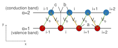
Figure 1: Schematic picture of two-band model with Coulomb interactions between chains. Red and blue circles indicate the lattice sites, $\alpha$ is the index of the chain, $b$ is the difference between the $x$-coordinates of the $i$-th site of two chains, and $c$ is the difference between $i$-th and ($i$-1)-th sites. $V_{b}$ and $V_{c}$ are the Coulomb interactions between the two chains.

To study EI, in this paper, we use a following two-band model Hamiltonian as shown in Fig. 1 matsuura :

$$\hat{\mathscr{H}}= \sum_{i}[\,(t\,\hat{c}^{\dagger}_{1,i}\,\hat{c}_{1,i+1}-t^{\prime}\,\hat{c}^{\dagger}_{2,i}\,\hat{c}_{2,i+1}+{\rm h.c.}\,)\,$$

$$+\left(-\epsilon-\mu\right)\hat{n}_{1,i}+\left(\epsilon-\mu\right)\hat{n}_{2,i}+V_{b}\,\hat{n}_{1,i}\,\hat{n}_{2,i}$$

$$+V_{c}\,\hat{n}_{1,i}\,\hat{n}_{2,i-1}\,]\,+\sum_{i,j,\alpha}V_{\rm{imp}}\left(x_{\alpha,i}-X_{j}\right)\hat{n}_{\alpha,i},$$ (4)

where $t$ ($t^{\prime}$) and $\epsilon$ are a transfer integral between the nearest-neighbor sites in the chain $\alpha=1$ ($\alpha=2$), and a one-body level of $i$-th site, respectively. $\hat{c}_{\alpha,i}$ ($\hat{c}_{\alpha,i}^{\dagger}$) is an annihilation (creation) operator at the $i$-th site of chain $\alpha$ where the spin degrees of freedom are neglected. $V_{b}$ and $V_{c}$ indicate the Coulomb interaction between $i$-th site in the chain $\alpha=1$ and $i$-th site in the chain $\alpha=2$ and that between $i$-th site in the chain $\alpha=1$ and ($i$-1)-th site in the chain $\alpha=2$. Figure 1 shows the positions of sites. $b$ ($c$) is the difference between the $x$-coordinates of the $i$-th site in the chain $\alpha=1$ and the $i$-th (($i$-1)-th) site in the chain $\alpha=2$. We set the lattice constant $a$ as $a=b+c$. $V_{\rm imp}\left(x_{\alpha,i}-X_{j}\right)$ is the randomly distributed impurity potential where $x_{\alpha,i}$ and $X_{j}$ are the $x$-coordinates of the position of the site and randomly distributed impurities, respectively.

The similar effective model has been suggested in Ref. matsuura . The model of Ref. matsuura corresponds to that for $c=a$, $b=0$ and $V_{c}=0$ in Eq. (4). As discussed below, the finite $b$ and $V_{c}$ are important to obtain the additional heat current due to the Coulomb interaction.

Using a mean-field approximation for EI and assuming that the order parameters are independent of the sites, i.e.,

$$\begin{split}\Delta_{b}=&-\frac{V_{b}}{N}\sum_{i}\langle\hat{c}^{\dagger}_{2,i}\,\hat{c}_{1,i}\rangle=-\frac{V_{b}}{N}\sum_{k}\langle\hat{c}^{\dagger}_{2,k}\,\hat{c}_{1,k}\rangle e^{-ikb},\\ \Delta_{c}=&-\frac{V_{c}}{N}\sum_{i}\langle\hat{c}^{\dagger}_{2,i-1}\,\hat{c}_{1,i}\rangle=-\frac{V_{c}}{N}\sum_{k}\langle\hat{c}^{\dagger}_{2,k}\,\hat{c}_{1,k}\rangle e^{ikc},\end{split}$$ (5)

with $N$ being the total number of sites, we obtain the following mean field Hamiltonian of EI

$$\hat{\mathscr{H}}_{\rm MF}= \sum_{k}\{\left(2t\,{\rm cos}ka-\epsilon-\mu\right)\hat{c}^{\dagger}_{1,k}\,\hat{c}_{1,k}$$

$$+\left(-2t^{\prime}\,{\rm cos}ka+\epsilon-\mu\right)\hat{c}^{\dagger}_{2,k}\,\hat{c}_{2,k}$$

$$+(\,\Delta_{k}\,\hat{c}^{\dagger}_{1,k}\,\hat{c}_{2,k}+{\rm h.c.})\}$$

$$+\sum_{k,q,\alpha}\frac{1}{N}\,\rho_{\rm imp}\left(q\right)v_{\rm imp}\left(q\right)\hat{c}^{\dagger}_{\alpha,k+q}\,\hat{c}_{\alpha,k},$$ (6)

where $\Delta_{k}\equiv\,\Delta_{b}\,e^{ikb}+\Delta_{c}\,e^{-ikc}$, $\rho_{\rm imp}\left(q\right)\equiv\sum_{i}e^{-iqX_{i}}$ and $v_{\rm imp}\left(q\right)\equiv\sum_{i}e^{-iq\left(x_{\alpha,i}-X\right)}\,V_{\rm imp}\left(x_{\alpha,i}-X\right)$.

By diagonalizing this Hamiltonian except for the impurity potential, we obtain

$$\hat{\mathscr{H}}_{\rm eff}=\sum_{k}\left(E_{k+}\,\hat{p}^{\dagger}_{k+}\,\hat{p}_{k+}+E_{k-}\,\hat{p}^{\dagger}_{k-}\,\hat{p}_{k-}\right),$$ (7)

where $\hat{p}_{k\pm}$ is an annihilation operator of a quasiparticle, and the quasiparticle energy is given by

$$E_{k\pm}= \left(t-t^{\prime}\right)\,{\rm cos}ka-\mu$$

$$\pm\sqrt{\left\{\left(t+t^{\prime}\right)\,{\rm cos}ka-\epsilon\right\}^{2}+\left|\Delta_{k}\right|^{2}}.$$ (8)

The unitary matrix satisfying $\left(\begin{array}[]{c}\hat{c}_{1,k}\\ \hat{c}_{2,k}\end{array}\right)\equiv\,\bm{U}\left(\begin{array}[]{c}\hat{p}_{k+}\\ \hat{p}_{k-}\end{array}\right)$ is

$$\bm{U}=\frac{1}{\sqrt{2X_{k}}}\left(\begin{array}[]{cc}\frac{\Delta_{k}}{\sqrt{X_{k}-Y_{k}}}&\frac{\Delta_{k}}{\sqrt{X_{k}+Y_{k}}}\\ \frac{X_{k}-Y_{k}}{\sqrt{X_{k}-Y_{k}}}&\frac{-X_{k}-Y_{k}}{\sqrt{X_{k}+Y_{k}}}\end{array}\right),$$ (11)

where $X_{k}$ and $Y_{k}$ are

$$\begin{split}X_{k}&\equiv\sqrt{\left\{\left(t+t^{\prime}\right)\,{\rm cos}ka-\epsilon\right\}^{2}+\left|\Delta_{k}\right|^{2}},\\ Y_{k}&\equiv\left(t+t^{\prime}\right)\,{\rm cos}ka-\epsilon.\end{split}$$ (12)

Using the effective Hamiltonian of Eq. (7), the self-consistent equations to obtain the order parameters of EI becomes

$$\Delta_{b}= -\frac{V_{b}}{2N}\sum_{k}\left(\Delta_{b}+\Delta_{c}\,e^{-ika}\right)\frac{f\left(E_{k+}\right)-f\left(E_{k-}\right)}{X_{k}},$$

$$\Delta_{c}= -\frac{V_{c}}{2N}\sum_{k}\left(\Delta_{b}\,e^{ika}+\Delta_{c}\right)\frac{f\left(E_{k+}\right)-f\left(E_{k-}\right)}{X_{k}}.$$ (13)

The chemical potential is now included in $E_{k\pm}$. Since we focus on the half-filling case in this paper, the chemical potential is determined by

$$\frac{1}{N}\sum_{k}\left\{f\left(E_{k+}\right)+f\left(E_{k-}\right)\right\}=1.$$ (14)

Solving Eqs. (13) and (14) self-consistently, we can obtain $\Delta_{b}$  ,  $\Delta_{c}$ and $\mu$. It is to be noted that the order parameters can be complex. However, we find that the phase difference between $\Delta_{b}$ and $\Delta_{c}$ does not occur in the parameters we used in this paper. Thus, we set the order parameters as real numbers.

Figure 2 shows the dispersion relations of normal state (black lines) and EI (red lines) at $T/t=0$ for several values of Hamiltonian parameters. We set $t^{\prime}=t$, $V_{b}=V_{c}=0.5t$, and $\epsilon=1.95t$ for Fig. 2(a) and $\epsilon=2.01t$ for Fig. 2(b), and $t^{\prime}=3t$, $V_{b}=V_{c}=2t$, and $\epsilon=3t$ for Fig. 2(c) and $\epsilon=4.2t$ for Fig. 2(d), respectively. The dispersion relations of the normal state indicate the semimetallic state for Figs. 2(a) and (c), or the semiconducting state for Figs. 2(b) and (d). When we consider the order parameters of EI, all the electronic states become the semiconducting states.

Figures 3(a) and (b) show the $\epsilon$ dependence of the transition temperature of EI. The parameters of Fig. 3(a) (Fig. 3(b)) are the same as that of Fig. 2(a) (Fig. 2(c)). As shown in Fig. 3(a) and (b), the transition temperature has a maximum at $(\epsilon-t-t^{\prime})/t\sim 0$. This $\epsilon$ behavior is the same as the result of Ref. matsuura .

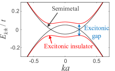
(a)

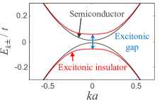
(b)

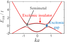
(c)

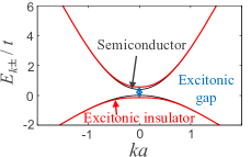
(d)

Figure 2: Dispersion relations of normal state (black line) and EI (red line) at $T/t=0$. The parameters are set as (a) $t^{\prime}=t$, $V_{b}=V_{c}=0.5t$, and $\epsilon=1.95t$, (b) $t^{\prime}=t$, $V_{b}=V_{c}=0.5t$, and $\epsilon=2.01t$, (c) $t^{\prime}=3t$, $V_{b}=V_{c}=2t$ and $\epsilon=3t$, and (d) $t^{\prime}=3t$, $V_{b}=V_{c}=2t$ and $\epsilon=4.2t$.

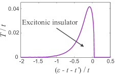
(a)

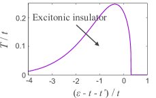
(b)

Figure 3: $\epsilon$ dependence of the transition temperature at (a) $t^{\prime}=t$ and $V_{b}=V_{c}=0.5t$ and (b) $t^{\prime}=3t$ and $V_{b}=V_{c}=2t$.

III Electric and heat current operators

The electric current density operator $\hat{\bm{j}}\left(\bm{r}\right)$ and the heat current density operator $\hat{\bm{j}}^{Q}\left(\bm{r}\right)$ are derived from the continuity equations linear

$$\frac{d\hat{\rho}\left(\bm{r}\right)}{dt}+{\rm div}\hat{\bm{j}}\left(\bm{r}\right)=0,\;\;\frac{d\hat{h}\left(\bm{r}\right)}{dt}+{\rm div}\hat{\bm{j}}^{Q}\left(\bm{r}\right)=0,$$ (15)

where $\hat{\rho}\left(\bm{r}\right)$ and $\hat{h}\left(\bm{r}\right)$ are the charge density and the Hamiltonian density ($\hat{\mathscr{H}}=\int d\bm{r}\,\hat{h}\left(\bm{r}\right)$), respectively.

In the preset model (Eq. (4)), the total electric current operator, $\hat{J}=\int d\bm{r}\hat{j}\left(\bm{r}\right)$, is given by

$$\hat{J}=\sum_{k,\alpha}j_{\alpha}\left(k\right)\,\hat{c}^{\dagger}_{\alpha,k}\,\hat{c}_{\alpha,k},$$ (16)

with

$$j_{1}\left(k\right)\equiv-\frac{2ea}{\hbar}t\,{\rm sin}ka,\;\;j_{2}\left(k\right)\equiv\,\frac{2ea}{\hbar}t^{\prime}\,{\rm sin}ka.$$ (17)

On the other hand, the total heat current operator,
$\hat{J}^{Q}=\int d\bm{r}\hat{j}^{Q}\left(\bm{r}\right)$, becomes

$$\hat{J}^{Q}= \sum_{k,\alpha}j^{Q}_{\alpha\alpha}\left(k\right)\hat{c}^{\dagger}_{\alpha,k}\,\hat{c}_{\alpha,k}$$

$$+\sum_{k,k^{\prime},q}j^{Q}_{V}\left(k,k^{\prime},q\right)\hat{c}^{\dagger}_{1,k+q}\,\hat{c}_{1,k}\,\hat{c}^{\dagger}_{2,k^{\prime}-q}\,\hat{c}_{2,k^{\prime}}$$

$$+\sum_{k,q,\alpha}j^{Q}_{{\rm imp}\alpha}\left(k,q\right)\hat{c}^{\dagger}_{\alpha,k+q}\,\hat{c}_{\alpha,k},$$ (18)

with

$$j^{Q}_{11}\left(k\right)\equiv-\frac{2a}{\hbar}t\,{\rm sin}ka\left(2t\,{\rm cos}ka-\epsilon-\mu\right),$$

$$j^{Q}_{22}\left(k\right)\equiv\frac{2a}{\hbar}t^{\prime}\,{\rm sin}ka\left(-2t^{\prime}\,{\rm cos}ka+\epsilon-\mu\right),$$

$$j^{Q}_{V}\left(k,k^{\prime},q\right)$$

$$\equiv -\frac{a}{\hbar}\left(t-t^{\prime}\right)\frac{1}{N}\Bigl{\{}\left(V_{b}e^{iqb}+V_{c}e^{-iqc}\right){\rm cos}\frac{q}{2}a\,{\rm sin}(k+\frac{q}{2})a$$

$$+\left(V_{b}e^{iq(b+\frac{a}{2})}+V_{c}e^{-iq(c+\frac{a}{2})}\right){\rm sin}(k^{\prime}-\frac{q}{2})a\Bigr{\}},$$

$$j^{Q}_{{\rm imp}1}\left(k,q\right)$$

$$\equiv -\frac{2a}{\hbar}t\frac{1}{N}\,\rho_{\rm imp}\left(q\right)v_{\rm imp}\left(q\right){\rm cos}\frac{q}{2}a\,{\rm sin}(k+\frac{q}{2})a,$$

$$j^{Q}_{{\rm imp}2}\left(k,q\right)$$

$$\equiv \frac{2a}{\hbar}t^{\prime}\frac{1}{N}\,\rho_{\rm imp}\left(q\right)v_{\rm imp}\left(q\right){\rm cos}\frac{q}{2}a\,{\rm sin}(k+\frac{q}{2})a.$$ (19)

The derivations of these operators together with the Hamiltonian density are shown in Appendix A. While $\hat{J}$ in Eq. (16) is a one-body current operator, the heat current operator $\hat{J}^{Q}$ in Eq. (18) is the many-body operator in the presence of the Coulomb interaction fukuyama .

As discussed in Appendix B, if we start from the mean field Hamiltonian of Eq. (6), we obtain a different expression of heat current operator. However, the heat current operator in Eq. (18) should be used to study the thermal conductivity, because it satisfies the continuity equation (15) without any approximations.

IV Additional heat current contribution in the EI phase

In this section, we study thermal conductivity based on the linear response theory within the mean-field approximation to clarify the additional contributions in the EI phase, which do not satisfy the SB relation in Eqs. (1).

In the mean-field approximation (6), the one-body Green’s function is given as

$$\mathscr{G}^{0}_{\alpha\alpha^{\prime}}\left(k,\tau\right) \equiv-\left\langle T_{\tau}\left[\,\hat{p}_{k\alpha}\left(\tau\right)\hat{p}^{\dagger}_{k\alpha^{\prime}}\left(0\right)\right]\right\rangle,$$ (20)

$$\bm{G}^{(0)}\left(k,i\epsilon_{n}\right) \equiv\left(\begin{array}[]{cc}\mathscr{G}^{0}_{\scriptscriptstyle++}\left(k,i\epsilon_{n}\right)&\mathscr{G}^{0}_{\scriptscriptstyle+-}\left(k,i\epsilon_{n}\right)\\ \mathscr{G}^{0}_{\scriptscriptstyle-+}\left(k,i\epsilon_{n}\right)&\mathscr{G}^{0}_{\scriptscriptstyle--}\left(k,i\epsilon_{n}\right)\end{array}\right)$$ (23)

$$=\left(\begin{array}[]{cc}\frac{1}{i\epsilon_{n}-E_{k+}}&0\\ 0&\frac{1}{i\epsilon_{n}-E_{k-}}\end{array}\right),$$ (26)

where $T_{\tau}$ is the standard $\tau$-ordering operator, and $\epsilon_{n}=(2n+1)\pi k_{B}T$ where $n$ is an integer. Taking into account the self-energy due to the impurity scattering

$$\bm{\Sigma}\left(k,i\epsilon_{n}\right)= -i\,{\rm sign}\left(\epsilon_{n}\right)\left(\begin{array}[]{cc}\Gamma_{1}&\Gamma_{3}\\ \Gamma_{3}&\Gamma_{2}\end{array}\right),$$ (29)

where $\Gamma_{1}$, $\Gamma_{2}$ and $\Gamma_{3}$ are real independent of $\epsilon_{n}$, Dyson’s equation leads to

$$\bm{G}\left(k,i\epsilon_{n}\right)={\scriptstyle\frac{1}{\left(i\epsilon_{n}-E_{k+}+i\,{\rm sign}\left(\epsilon_{n}\right)\Gamma_{1}\right)\left(i\epsilon_{n}-E_{k-}+i\,{\rm sign}\left(\epsilon_{n}\right)\Gamma_{2}\right)+\Gamma_{3}^{2}}}\left(\begin{array}[]{cc}i\epsilon_{n}-E_{k-}+i\,{\rm sign}\left(\epsilon_{n}\right)\Gamma_{2}&-i\,{\rm sign}\left(\epsilon_{n}\right)\Gamma_{3}\\ -i\,{\rm sign}\left(\epsilon_{n}\right)\Gamma_{3}&i\epsilon_{n}-E_{k+}+i\,{\rm sign}\left(\omega_{n}\right)\Gamma_{1}\end{array}\right).$$ (32)

In this paper, the values of $\Gamma_{1}$ $\Gamma_{2}$ and $\Gamma_{3}$ are estimated by calculating the self-energy in the absence of interactions from Dyson’s Equation as follows

$$\begin{split}\Gamma_{1}=&\frac{an_{i}v^{2}}{2X_{k}}\left(\frac{X_{k}+Y_{k}}{\sqrt{4t^{2}-\left(\epsilon+\mu\right)^{2}}}+\frac{X_{k}-Y_{k}}{\sqrt{4t^{\prime 2}-\left(\epsilon-\mu\right)^{2}}}\right),\\ \Gamma_{2}=&\frac{an_{i}v^{2}}{2X_{k}}\left(\frac{X_{k}-Y_{k}}{\sqrt{4t^{2}-\left(\epsilon+\mu\right)^{2}}}+\frac{X_{k}+Y_{k}}{\sqrt{4t^{\prime 2}-\left(\epsilon-\mu\right)^{2}}}\right),\\ \Gamma_{3}=&\frac{an_{i}v^{2}}{2X_{k}}\left(\frac{\left|\Delta_{k}\right|}{\sqrt{4t^{2}-\left(\epsilon+\mu\right)^{2}}}+\frac{\left|\Delta_{k}\right|}{\sqrt{4t^{\prime 2}-\left(\epsilon-\mu\right)^{2}}}\right).\end{split}$$ (33)

Here, $n_{i}$ is the impurity density, and we assumed that $v_{\rm imp}\left(q\right)=v$, ignoring the $q$ dependence of $v_{\rm imp}\left(q\right)$.

We also apply the mean-field approximation to the heat current operator to obtain

$$\hat{J}^{Q}_{{\rm MF}}= \sum_{k,\alpha,\alpha^{\prime}}j^{Q}_{\alpha\alpha^{\prime}}\left(k\right)\hat{c}^{\dagger}_{\alpha,k}\,\hat{c}_{\alpha^{\prime},k}$$

$$+\sum_{k,q,\alpha}j^{Q}_{{\rm imp}\alpha}\left(k,q\right)\hat{c}^{\dagger}_{\alpha,k+q}\,\hat{c}_{\alpha,k},$$ (34)

where $j^{Q}_{12}$ and $j^{Q}_{21}$ are

$$j^{Q}_{12}\left(k\right)=\overline{j^{Q}_{21}\left(k\right)}$$

$$\equiv -\frac{a}{\hbar}\left(t-t^{\prime}\right)\Bigl{\{}\Delta_{k}\,{\rm sin}ka+\frac{i}{4}\left(\frac{V_{c}}{V_{b}}\Delta_{b}\,e^{-ikc}-\frac{V_{b}}{V_{c}}\Delta_{c}\,e^{ikb}\right)$$

$$-\frac{i}{2}\left(\Delta_{b}\,e^{ikb}-\Delta_{c}\,e^{-ikc}\right){\rm cos}ka\Bigr{\}}.$$ (35)

We will proceed with the calculation assuming that the effect of impurities is sufficiently small. From Eq. (19), it can be seen that the heat current $j^{Q}_{{\rm imp}1}\left(k,q\right)$ and $j^{Q}_{{\rm imp}2}\left(k,q\right)$ due to impurities only have effects of the order of $\mathcal{O}\left(v_{\rm imp}\right)$ or $\mathcal{O}\left(v_{\rm imp}^{2}\right)$, which is smaller than the other heat current. Therefore, the heat current due to impurities will be ignored in following calculations. We also ignore the vertex correction due to impurities as well, since it only affects the current and heat current operators of the order of $\mathcal{O}\left(v_{\rm imp}^{2}\right)$.

Using the annihilation and creation operators of quasiparticle, $\hat{p}^{\dagger}_{k\alpha}$ and $\hat{p}_{k\alpha}$, the electric current and heat current operators are written as

$$\begin{split}\hat{J}=&\sum_{k}\left(\begin{array}[]{cc}\hat{p}^{\dagger}_{k+}&\hat{p}^{\dagger}_{k-}\end{array}\right)\bm{\Gamma}\left(k\right)\left(\begin{array}[]{c}\hat{p}_{k+}\\ \hat{p}_{k-}\end{array}\right),\\ \hat{J}^{Q}_{\rm MF}=&\sum_{k}\left(\begin{array}[]{cc}\hat{p}^{\dagger}_{k+}&\hat{p}^{\dagger}_{k-}\end{array}\right)\bm{\Gamma}^{Q}\left(k\right)\left(\begin{array}[]{c}\hat{p}_{k+}\\ \hat{p}_{k-}\end{array}\right),\end{split}$$ (36)

where $\bm{\Gamma}=\bm{U}^{\dagger}\left(\begin{array}[]{cc}j_{1}&0\\ 0&j_{2}\end{array}\right)\bm{U}$, $\bm{\Gamma}^{Q}=\bm{U}^{\dagger}\left(\begin{array}[]{cc}j^{Q}_{11}&j^{Q}_{12}\\ j^{Q}_{21}&j^{Q}_{22}\end{array}\right)\bm{U}$.

$L_{11}$ is obtained by the $\hat{J}$-$\hat{J}$ correlation

$$\Phi_{11}\left(\tau\right)=\frac{1}{aN}\left\langle T_{\tau}\left[\,\hat{J}\left(\tau\right)\hat{J}\left(0\right)\right]\right\rangle$$

$$= -\frac{1}{aN}\sum_{k}{\rm Tr}\left[\bm{\Gamma}\left(k\right)\bm{G}\left(k,\tau\right)\bm{\Gamma}\left(k\right)\bm{G}\left(k,-\tau\right)\right],$$ (37)

and its Fourier transform

$$\Phi_{11}\left(i\omega_{\lambda}\right)= -\frac{k_{B}T}{aN}\sum_{k}\sum_{n}{\rm Tr}[\bm{\Gamma}\left(k\right)\bm{G}\left(k,i\epsilon_{n}\right)$$

$$\times\bm{\Gamma}\left(k\right)\bm{G}\left(k,i\epsilon_{n}-i\omega_{\lambda}\right)].$$ (38)

Here, $\omega_{\lambda}=2\lambda\pi k_{B}T$ and $\lambda$ is an integer.

By performing the analytic continuation ($i\omega_{\lambda}\rightarrow\hbar\omega+i\delta$), we can obtain

$$L_{11}=\lim_{\omega\to 0}\frac{\Phi_{11}\left(\hbar\omega+i\delta\right)-\Phi_{11}\left(0\right)}{i\omega}.$$ (39)

Similarly, $L_{21}$, $L_{22}$ can be calculated by

$$\Phi_{21}\left(i\omega_{\lambda}\right)= -\frac{k_{B}T}{aN}\sum_{k}\sum_{n}{\rm Tr}[\bm{\Gamma}^{Q}\left(k\right)\bm{G}\left(k,i\epsilon_{n}\right)$$

$$\times\bm{\Gamma}\left(k\right)\bm{G}\left(k,i\epsilon_{n}-i\omega_{\lambda}\right)],$$ (40)

$$\Phi_{22}\left(i\omega_{\lambda}\right)= -\frac{k_{B}T}{aN}\sum_{k}\sum_{n}{\rm Tr}[\bm{\Gamma}^{Q}\left(k\right)\bm{G}\left(k,i\epsilon_{n}\right)$$

$$\times\bm{\Gamma}^{Q}\left(k\right)\bm{G}\left(k,i\epsilon_{n}-i\omega_{\lambda}\right)].$$ (41)

Equations. (40) and (41) correspond to the Feynman diagrams shown in Fig. 4.

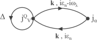
(a)

(b)

Figure 4: Feynman diagrams for heat currents including interactions.

We can see that the dominant contributions are in the order of $\mathcal{O}\left(1/\Gamma_{1}\right)$, $\mathcal{O}\left(1/\Gamma_{2}\right)$ and $\mathcal{O}\left(1/\Gamma_{3}\right)$. Then, ignoring the higher order of $\mathcal{O}\left(\Gamma_{1}\right)$, $\mathcal{O}\left(\Gamma_{2}\right)$ and $\mathcal{O}\left(\Gamma_{3}\right)$, we obtain the correlation functions as follows.

$$L_{11}$$

$$= \frac{e^{2}a^{2}}{4\pi\hbar}\int dk\left(-f^{\prime}\left(E_{k+}\right)\frac{\sigma_{k+}^{2}}{\Gamma_{1}}-f^{\prime}\left(E_{k-}\right)\frac{\sigma_{k-}^{2}}{\Gamma_{2}}\right),$$ (42a)

$$L_{21}$$

$$= \frac{ea^{2}}{4\pi\hbar}\int dk\left(-E_{k+}f^{\prime}\left(E_{k+}\right)\frac{\sigma_{k+}^{2}}{\Gamma_{1}}-E_{k-}f^{\prime}\left(E_{k-}\right)\frac{\sigma_{k-}^{2}}{\Gamma_{2}}\right)$$

$$+\frac{ea^{2}}{4\pi\hbar}\int dk\left(-f^{\prime}\left(E_{k+}\right)\frac{g_{k}\sigma_{k+}}{\Gamma_{1}}+f^{\prime}\left(E_{k-}\right)\frac{g_{k}\sigma_{k-}}{\Gamma_{2}}\right),$$ (42b)

$$L_{22}$$

$$= \frac{a^{2}}{4\pi\hbar}\int dk\left(-E_{k+}^{2}f^{\prime}\left(E_{k+}\right)\frac{\sigma_{k+}^{2}}{\Gamma_{1}}-E_{k-}^{2}f^{\prime}\left(E_{k-}\right)\frac{\sigma_{k-}^{2}}{\Gamma_{2}}\right)$$

$$+\frac{a^{2}}{2\pi\hbar}\int dk\Bigl{(}-E_{k+}f^{\prime}\left(E_{k+}\right)\frac{g_{k}\sigma_{k+}}{\Gamma_{1}}$$

$$+E_{k-}f^{\prime}\left(E_{k-}\right)\frac{g_{k}\sigma_{k-}}{\Gamma_{2}}\Bigr{)}$$

$$+\frac{a^{2}}{4\pi\hbar}\int dk\left(-f^{\prime}\left(E_{k+}\right)\frac{g_{k}^{2}}{\Gamma_{1}}-f^{\prime}\left(E_{k-}\right)\frac{g_{k}^{2}}{\Gamma_{2}}\right),$$ (42c)

where $\sigma_{k\pm}$ and $g_{k}$ are

$$\sigma_{k\pm} \equiv \frac{{\rm sin}ka}{X_{k}}\left\{\left(X_{k}\pm Y_{k}\right)t-\left(X_{k}\mp Y_{k}\right)t^{\prime}\right\},$$ (43)

$$g_{k} \equiv \frac{t-t^{\prime}}{4X_{k}}\Bigl{\{}\left(\frac{V_{c}}{V_{b}}\Delta_{b}^{2}+\frac{V_{b}}{V_{c}}\Delta_{c}^{2}\right){\rm sin}ka$$ (44)

$$+2\Delta_{b}\Delta_{c}\,{\rm sin}2ka\Bigr{\}}.$$

Derivations of Eqs. (42) are given in Appendix C.

$L_{21}$ and $L_{22}$ differ from $L_{11}$ in that $g_{k}$ appears in the integrand. In other words, the first term in $L_{21}$ and $L_{22}$ are expressed by the SB relations. In contrast, the second term in $L_{21}$ and the second and third terms in $L_{22}$ are not expressed by the SB relations. Therefore, these terms give the additional contributions to the thermal conductivity in the EI phase. This is the main result of this paper, and we will discuss it more in detail in the next section.

Before going into details, let us see the magnitude of this newly-found additional contributions. Figures 5(a) - (b) (5(c) - (d)) show the temperature dependence of $L_{11}$ and $\kappa$ at $t^{\prime}=t$, $V_{b}=V_{c}=0.5t$, and $\epsilon=1.95t$ (at $t^{\prime}=3t$, $V_{b}=V_{c}=2t$, and $\epsilon=3t$). The portion of $\kappa$ that is related to $g_{k}$ is indicated by the blue line, the others by the black line, and the total by the red line.

It is found that the contribution of $g_{k}$ to the thermal conductivity is present below the transition temperature. When $t=t^{\prime}$ the thermal conductivity follows the SB relation because $g_{k}=0$ (Fig. 5(b)), but when $t\neq t^{\prime}$, it may be visible depending on the parameters (Fig. 5(d)). This is the thermal conductivity produced by the additional heat current driven by EI.

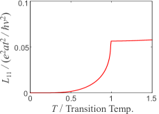
(a)

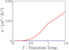
(b)

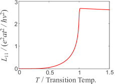
(c)

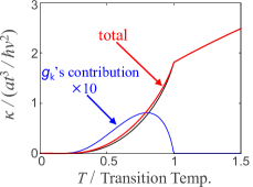
(d)

Figure 5: Temperature dependence on (a) $L_{11}$ and (b) $\kappa$ at $t^{\prime}=t$, $V_{b}=V_{c}=0.5t$, $\epsilon=1.95t$, and (c) $L_{11}$ and (d) $\kappa$ at $t^{\prime}=3t$, $V_{b}=V_{c}=2t$, $\epsilon=3t$. Blue, black, and red line indicates the contribution from $g_{k}\times 10$, other terms, and total, respectively.

V Discussions

As mentioned in Sect. 1, when the heat current operator, $\widetilde{\hat{J}^{Q}}\left(\tau\right)$, can be written in the form of an imaginary-time derivative of the electric current
($\hat{J}\left(\tau,\tau^{\prime}\right)=\sum_{k}\left\{j\left(k\right)\hat{c}^{\dagger}_{k}\left(\tau\right)\hat{c}_{k}\left(\tau^{\prime}\right)\right\}$) as

$$\widetilde{\hat{J}^{Q}}\left(\tau\right)=\lim_{\tau^{\prime}\to\tau}\frac{1}{2}\left(\frac{\partial}{\partial\tau}-\frac{\partial}{\partial\tau^{\prime}}\right)\hat{J}\left(\tau,\tau^{\prime}\right),$$ (45)

$L_{11}$, $L_{21}$, and $L_{22}$ are expressed by Eqs. (1) jonson ; fukuyama , where $\hat{c}_{k}\left(\tau\right)$ is an annihilation operator with an imaginary-time dependence.

In the present case of mean-field approximation, if we consider that the imaginary-time derivative of $\tau$ and $\tau^{\prime}$ are given by the mean field Hamiltonian (6) as

$$\begin{split}\frac{\partial}{\partial\tau}\hat{J}\left(\tau,\tau^{\prime}\right)=\sum_{k}j\left(k\right)\left[\hat{\mathscr{H}_{\rm MF}}\left(\tau\right),\hat{c}^{\dagger}_{k}\left(\tau\right)\right]\hat{c}_{k}\left(\tau^{\prime}\right),\\ \frac{\partial}{\partial\tau^{\prime}}\hat{J}\left(\tau,\tau^{\prime}\right)=\sum_{k}j\left(k\right)\hat{c}^{\dagger}_{k}\left(\tau\right)\left[\hat{\mathscr{H}_{\rm MF}}\left(\tau^{\prime}\right),\hat{c}_{k}\left(\tau^{\prime}\right)\right].\end{split}$$ (46)

We obtain

$$\widetilde{\hat{J}^{Q}}\left(\tau\right)= \lim_{\tau^{\prime}\to\tau}\frac{1}{2}\left(\frac{\partial}{\partial\tau}-\frac{\partial}{\partial\tau^{\prime}}\right)\hat{J}\left(\tau,\tau^{\prime}\right)$$

$$= \sum_{k,\alpha,\alpha^{\prime}}j^{\prime Q}_{\alpha\alpha^{\prime}}\left(k\right)\hat{c}^{\dagger}_{\alpha,k}\left(\tau\right)\hat{c}_{\alpha^{\prime},k}\left(\tau\right)$$

$$+\sum_{k,q,\alpha}j^{Q}_{{\rm imp}\alpha}\left(k,q\right)\hat{c}^{\dagger}_{\alpha,k+q}\left(\tau\right)\hat{c}_{\alpha,k}\left(\tau\right),$$ (47)

where

$$j^{\prime Q}_{11}\left(k\right)\equiv j^{Q}_{11}\left(k\right),\;\;j^{\prime Q}_{22}\left(k\right)\equiv j^{Q}_{22}\left(k\right),$$

$$j^{\prime Q}_{12}\left(k\right)= \overline{j^{\prime Q}_{21}\left(k\right)}\equiv-\frac{a}{\hbar}\left(t-t^{\prime}\right)\Delta_{k}\,{\rm sin}ka.$$ (48)

When we use $\widetilde{\hat{J}^{Q}}$ instead of $\hat{J}^{Q}$, we obtain the first term in $L_{21}$ and $L_{22}$ in Eqs. (42). Therefore, this is consistent with the argument by Jonson-Mahan jonson that the heat current operator $\widetilde{\hat{J}^{Q}}$ leads to SB relations.

In other words, the contributions which violate the SB relations appears in $L_{21}$ and $L_{22}$, that is $g_{k}$, from the second and third terms in $j^{Q}_{12}$ in Eq. (19), which originate from the two types of Coulomb interactions. Furthermore, this $g_{k}$ is represented by the order parameters of EI, and it contributes not to the electrical conductivity but to the thermal conductivity below the transition temperature.

Although the effect of $g_{k}$ is small in the present model, this term gives essentially new contribution to the thermal conductivity, which is beyond the SB relations. It is to be noted that $g_{k}$ does not appear when one type of interaction is considered. It has already been pointed out that such terms beyond the SB relations do not appear in the Hubbard model kontani , and the same argument can be made in this model by mapping the two bands to the spin direction. In other words, considering the two types of interactions is essential to obtain heat current beyond the SB relations.

Finally, we discuss the relationship between the additional contribution to the thermal conductivity and the heat current of excitions. As mentioned in the introduction, the thermal transport due to excitons is expected to show the drastic features, because excitons do not have electronic charges, but have energies contributing to the heat current. The heat current due to excitons is not included in the previous studies zittartz3 ; kurihara , because they are based on the SB relations. However, we find the additional thermal conductivity which does not satisfy the SB relations. Furthermore, additional thermal conductivity is related to the order parameters of EI. Therefore, it is suggested that the contribution from the heat current carried by excitons is included in additional thermal conductivity. Such theoretical understanding of the exciton’s heat current could provide the basis for the experimental determination of the EI state.

VI Conclusion

We study the thermal conductivity in EI using a simple quasi one-dimensional two-band model with the two types of Coulomb interactions between these bands. First, we obtained the heat current operator microscopically and clarified that it can not be written in the form of an imaginary-time derivative of the electric current operator as Eqs. (19) and (48). In other words, by considering two types of interactions, additional heat current operator owing to the excitonic phase transition exists, which is different from previous studies zittartz3 ; kurihara . Then, we studied the linear response theory of $L_{11}$, $L_{21}$, and $L_{22}$ within a mean-field scheme, and clarified that abovementioned additional heat current operator gives contributions in $L_{21}$ and $L_{22}$ which are not expressed in the form of Eqs. (1b) and (1c), or which are beyond the SB relations.

Appendix A Derivations of Eqs. (16) and (18) together with the Hamiltonian density

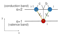
(a) $\hat{h}_{i}$

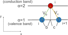
(b) $\hat{h}_{i+\frac{1}{2}}$

Figure 6: Schematic picture of the local (a) $i$-th site, (b) ($i$+1/2)-th site. For the local $i$-th site (($i$+1/2)-th site), we consider hopping in both directions from the $i$-th site in band 1 (band 2), and hopping between the ($i$-1)-th site and the $i$-th site in band 2 (between the $i$-th site and the ($i$+1)-th site in band 1).

In the preset model (Eq. (4)), the Hamiltonian density, $\hat{h}_{i}$ and $\hat{h}_{i+\frac{1}{2}}$, are obtained as

$$\hat{h}_{i}= \left(\frac{t}{2}\hat{c}^{\dagger}_{1,i}\,\hat{c}_{1,i+1}+\frac{t}{2}\hat{c}^{\dagger}_{1,i-1}\,\hat{c}_{1,i}-t^{\prime}\hat{c}^{\dagger}_{2,i-1}\,\hat{c}_{2,i}+{\rm h.c.}\right)$$

$$+\left(-\epsilon-\mu\right)\hat{n}_{1,i}+\frac{1}{2}\left(\epsilon-\mu\right)\left(\hat{n}_{2,i}+\hat{n}_{2,i-1}\right)$$

$$+V_{b}\,\hat{n}_{1,i}\,\hat{n}_{2,i}+V_{c}\,\hat{n}_{1,i}\,\hat{n}_{2,i-1}$$

$$+\sum_{j}\bigl{\{}V_{{\rm imp}}\left(x_{1,i}-X_{j}\right)\hat{n}_{1,i}+V_{{\rm imp}}\left(x_{2,i}-X_{j}\right)\frac{\hat{n}_{2,i}}{2}$$

$$+V_{{\rm imp}}\left(x_{2,i-1}-X_{j}\right)\frac{\hat{n}_{2,i-1}}{2}\bigr{\}},$$ (49)

$$\hat{h}_{i+\frac{1}{2}}= \left(t\hat{c}^{\dagger}_{1,i}\,\hat{c}_{1,i+1}-\frac{t^{\prime}}{2}\hat{c}^{\dagger}_{2,i-1}\,\hat{c}_{2,i}-\frac{t^{\prime}}{2}\hat{c}^{\dagger}_{2,i}\,\hat{c}_{2,i+1}+{\rm h.c.}\right)$$

$$+\frac{1}{2}\left(-\epsilon-\mu\right)\left(\hat{n}_{1,i+1}+\hat{n}_{1,i}\right)+\left(\epsilon-\mu\right)\hat{n}_{2,i}$$

$$+V_{b}\,\hat{n}_{1,i}\,\hat{n}_{2,i}+V_{c}\,\hat{n}_{1,i+1}\,\hat{n}_{2,i}$$

$$+\sum_{j}\bigl{\{}V_{{\rm imp}}\left(x_{1,i+1}-X_{j}\right)\frac{\hat{n}_{1,i+1}}{2}$$

$$+V_{{\rm imp}}\left(x_{1,i}-X_{j}\right)\frac{\hat{n}_{1,i}}{2}+V_{{\rm imp}}\left(x_{2,i}-X_{j}\right)\hat{n}_{2,i}\bigr{\}}.$$ (50)

Figure 6 shows the schematic picture of the Hamiltonian density. Using Eqs. (15), (49) and (50), the electric and the heat current density operators are expressed as

$$\begin{split}\frac{ie}{\hbar}\left[\frac{\hat{n}_{1,i}+\hat{n}_{2,i}}{a},\hat{\mathscr{H}}\right]=&\frac{2}{a}\left(\hat{j}_{i+\frac{1}{4}}-\hat{j}_{i-\frac{1}{4}}\right),\\ \frac{ie}{\hbar}\left[\frac{\hat{n}_{1,i+1}+\hat{n}_{2,i}}{a},\hat{\mathscr{H}}\right]=&\frac{2}{a}\left(\hat{j}_{i+\frac{3}{4}}-\hat{j}_{i+\frac{1}{4}}\right),\\ \frac{i}{\hbar}\left[\frac{\hat{h}_{i}}{a},\hat{\mathscr{H}}\right]=&\frac{2}{a}\left(\hat{j}^{Q}_{i+\frac{1}{4}}-\hat{j}^{Q}_{i-\frac{1}{4}}\right),\\ \frac{i}{\hbar}\left[\frac{\hat{h}_{i+\frac{1}{2}}}{a},\hat{\mathscr{H}}\right]=&\frac{2}{a}\left(\hat{j}^{Q}_{i+\frac{3}{4}}-\hat{j}^{Q}_{i+\frac{1}{4}}\right).\end{split}$$ (51)

Then, the total electric current and the total heat current operators become

$$\hat{J}= \frac{a}{2}\,\sum_{i}\left(\hat{j}_{i+\frac{1}{4}}+\hat{j}_{i+\frac{3}{4}}\right),\;\;\hat{J}^{Q}= \frac{a}{2}\,\sum_{i}\left(\hat{j}^{Q}_{i+\frac{1}{4}}+\hat{j}^{Q}_{i+\frac{3}{4}}\right)$$ (52)

As a result, we obtain Eqs. (16) and (18).

Appendix B Discussion on the derivation of heat current operator

The electric and heat current operators should be uniquely determined once the Hamiltonian is determined, and it should be determined independently of the mean-field approximation. Therefore, the current operators should not be calculated using the mean field Hamiltonian of Eq. (6), but should be calculated using the original Hamiltonian of Eq. (4) before the mean-field approximation is applied to the heat current operator.

In fact, the electric and heat current operators calculated using the mean field Hamiltonian (6), $\hat{J}^{\prime}_{{\rm MF}}$ and $\hat{J}^{\prime Q}_{{\rm MF}}$, are

$$\hat{J}^{\prime}_{{\rm MF}}= \sum_{k,\alpha,\alpha^{\prime}}j_{\alpha\alpha^{\prime}}\left(k\right)\hat{c}^{\dagger}_{\alpha,k}\,\hat{c}_{\alpha^{\prime},k},$$ (53)

with

$$j_{11}\left(k\right)\equiv j_{1}\left(k\right),\;\;j_{22}\left(k\right)\equiv j_{2}\left(k\right),$$

$$j_{12}\left(k\right)=\overline{j_{21}\left(k\right)}\equiv\frac{iea}{2\hbar}\left(\Delta_{b}e^{ikb}-\Delta_{c}e^{-ikc}\right),$$ (54)

and

$$\hat{J}^{\prime Q}_{{\rm MF}}= \sum_{k,\alpha,\alpha^{\prime}}j^{Q}_{{\rm MF}\alpha\alpha^{\prime}}\left(k\right)\hat{c}^{\dagger}_{\alpha,k}\,\hat{c}_{\alpha^{\prime},k}$$

$$+\sum_{k,q,\alpha,\alpha^{\prime}}j^{Q}_{{\rm imp}\alpha\alpha^{\prime}}\left(k,q\right)\,\hat{c}^{\dagger}_{\alpha,k+q}\,\hat{c}_{\alpha^{\prime},k},$$ (55)

with

$$j^{Q}_{{\rm MF}11}\left(k\right)\equiv j^{Q}_{11}\left(k\right)-\frac{a}{\hbar}\Delta_{b}\,\Delta_{c}\,{\rm sin}ka,$$

$$j^{Q}_{{\rm MF}22}\left(k\right)\equiv j^{Q}_{22}\left(k\right)-\frac{a}{\hbar}\Delta_{b}\,\Delta_{c}\,{\rm sin}ka,$$

$$j^{Q}_{{\rm MF}12}\left(k\right)=\overline{j^{Q}_{{\rm MF}21}}\left(k\right)$$

$$\equiv -\frac{a}{\hbar}\left(t-t^{\prime}\right)\Delta_{k}\,{\rm sin}ka$$

$$+\frac{ia}{2\hbar}\left(\Delta_{b}e^{ikb}-\Delta_{c}e^{-ikc}\right)\left\{\left(t-t^{\prime}\right){\rm cos}ka-\mu\right\},$$

$$j^{Q}_{{\rm imp}11}\left(k\right)\equiv j^{Q}_{{\rm imp}1}\left(k\right),\;\;j^{Q}_{{\rm imp}22}\left(k,q\right)\equiv j^{Q}_{{\rm imp}2}\left(k\right),$$

$$j^{Q}_{{\rm imp}12}\left(k,q\right)=\overline{j^{Q}_{{\rm imp}21}}\left(k\right)$$

$$\equiv \frac{1}{2}\Delta_{b}\,e^{ikb}\left(1+e^{iqb}\right)-\frac{1}{2}\Delta_{c}\,e^{-ikc}\left(1+e^{-iqc}\right).$$ (56)

These expressions are different from Eq. (19). Furthermore, if we use these operators $\hat{J_{\rm MF}^{\prime}}$ and $\hat{J^{\prime Q}_{\rm MF}}$, we obtain various additional terms compared with Eq. (42).

Like this, it is necessary to pay attention to the order of the calculation of the heat current operator and the application of the mean-field approximation.

Appendix C Derivations of Eqs. (42)

When we define $\Phi^{\alpha\beta}_{\gamma\delta}\left(k,\omega\right)$ as an analytic continuation ( $i\omega_{\lambda}\rightarrow\hbar\omega+i\delta$) to $\sum_{n}\mathscr{G}_{\alpha\beta}\left(k\,,i\epsilon_{n}\right)\mathscr{G}_{\gamma\delta}\left(k\,,i\epsilon_{n}-i\omega_{\lambda}\right)$ , the product of the Green’s function, we can calculate Eq. (39) by calculating

$$\sigma^{\alpha\beta}_{\gamma\delta}\left(k\right)\equiv\left.\frac{\Phi^{\alpha\beta}_{\gamma\delta}\left(k,\omega\right)-\Phi^{\alpha\beta}_{\gamma\delta}\left(k,\omega=0\right)}{i\omega}\right|_{\omega\rightarrow 0}.$$ (57)

Here, we calculate $\sigma^{\scriptscriptstyle++}_{\scriptscriptstyle++}\left(k\right)$ as an example. Using the Green’s function in Eq. (32) and replacing the sum of the Matsubara frequencies with the complex integral, we obtain

$$\sum_{n}\,\mathscr{G}_{\scriptscriptstyle++}\left(k,i\epsilon_{n}-i\omega_{\lambda}\right)\mathscr{G}_{\scriptscriptstyle++}\left(k,i\epsilon_{n}\right)$$

$$= -\frac{1}{2\pi ik_{B}T}\int^{\infty}_{-\infty}dx\,\Bigl{[}\,f\left(x+i\omega_{\lambda}\right)\Bigl{\{}{\scriptstyle\frac{x-E_{k-}+i\Gamma_{2}}{\left(x-E_{k+}+i\Gamma_{1}\right)\left(x-E_{k-}+i\Gamma_{2}\right)+\Gamma_{3}^{2}}\frac{x+i\omega_{\lambda}-E_{k-}+i\Gamma_{2}}{\left(x+i\omega_{\lambda}-E_{k+}+i\Gamma_{1}\right)\left(x+i\omega_{\lambda}-E_{k-}+i\Gamma_{2}\right)+\Gamma_{3}^{2}}}$$

$${\scriptstyle-\frac{x-E_{k-}-i\Gamma_{2}}{\left(x-E_{k+}-i\Gamma_{1}\right)\left(x-E_{k-}-i\Gamma_{2}\right)+\Gamma_{3}^{2}}\frac{x+i\omega_{\lambda}-E_{k-}+i\Gamma_{2}}{\left(x+i\omega_{\lambda}-E_{k+}+i\Gamma_{1}\right)\left(x+i\omega_{\lambda}-E_{k-}+i\Gamma_{2}\right)+\Gamma_{3}^{2}}}\Bigr{\}}$$

$$+f\left(x\right)\Bigl{\{}{\scriptstyle\frac{x-i\omega_{\lambda}-E_{k-}-i\Gamma_{2}}{\left(x-i\omega_{\lambda}-E_{k+}-i\Gamma_{1}\right)\left(x-i\omega_{\lambda}-E_{k-}-i\Gamma_{2}\right)+\Gamma_{3}^{2}}\frac{x-E_{k-}+i\Gamma_{2}}{\left(x-E_{k+}+i\Gamma_{1}\right)\left(x-E_{k-}+i\Gamma_{2}\right)+\Gamma_{3}^{2}}}$$

$${\scriptstyle-\frac{x-i\omega_{\lambda}-E_{k-}-i\Gamma_{2}}{\left(x-i\omega_{\lambda}-E_{k+}-i\Gamma_{1}\right)\left(x-i\omega_{\lambda}-E_{k-}-i\Gamma_{2}\right)+\Gamma_{3}^{2}}\frac{x-E_{k-}-i\Gamma_{2}}{\left(x-E_{k+}-i\Gamma_{1}\right)\left(x-E_{k-}-i\Gamma_{2}\right)+\Gamma_{3}^{2}}}\Bigr{\}}\,\Bigr{]}$$

$$= \frac{2}{\pi k_{B}T}\int^{\infty}_{-\infty}dx\,f\left(x\right)\Bigl{[}{\scriptstyle\frac{\left\{\Gamma_{1}\left(x-E_{k-}\right)^{2}+\Gamma_{1}\Gamma_{2}^{2}-\Gamma_{2}\Gamma_{3}^{2}\right\}}{\left\{\left(x-E_{k+}+i\Gamma_{1}\right)\left(x-E_{k-}+i\Gamma_{2}\right)+\Gamma_{3}^{2}\right\}\left\{\left(x-E_{k+}-i\Gamma_{1}\right)\left(x-E_{k-}-i\Gamma_{2}\right)+\Gamma_{3}^{2}\right\}}}$$

$${\scriptstyle\times\frac{\left(x-E_{k+}\right)\left\{\left(x-E_{k-}\right)^{2}-\left(i\omega_{\lambda}+i\Gamma_{2}\right)^{2}\right\}+\Gamma_{3}^{2}\left(x-E_{k-}\right)}{\left\{\left(x+i\omega_{\lambda}-E_{k+}+i\Gamma_{1}\right)\left(x+i\omega_{\lambda}-E_{k-}+i\Gamma_{2}\right)+\Gamma_{3}^{2}\right\}\left\{\left(x-i\omega_{\lambda}-E_{k+}-i\Gamma_{1}\right)\left(x-i\omega_{\lambda}-E_{k-}-i\Gamma_{2}\right)+\Gamma_{3}^{2}\right\}}}\Bigr{]}.$$ (58)

By performing analytic continuation ($i\omega_{\lambda}\rightarrow\hbar\omega+i\delta$), we obtain

$$\sigma^{\scriptscriptstyle++}_{\scriptscriptstyle++}\left(k\right)=\frac{4\hbar}{\pi k_{B}T}\int^{\infty}_{-\infty}dx\,f\left(x\right)\frac{\begin{array}[]{l}{\scriptstyle\{\,\Gamma_{1}^{2}\left(x-E_{k+}\right)\left(x-E_{k-}\right)^{6}-\Gamma_{1}\Gamma_{2}\Gamma_{3}^{2}\left(x-E_{k+}\right)^{2}\left(x-E_{k-}\right)^{3}}\\ {\scriptstyle+\left(3\Gamma_{1}^{2}\Gamma_{2}^{2}-2\Gamma_{1}\Gamma_{2}\Gamma_{3}^{2}-\Gamma_{1}^{2}\Gamma_{3}^{2}\right)\left(x-E_{k+}\right)\left(x-E_{k-}\right)^{4}+\Gamma_{1}^{2}\Gamma_{3}^{2}\left(x-E_{k-}\right)^{5}\}}\end{array}}{{\scriptstyle\left\{\left(x-E_{k+}+i\Gamma_{1}\right)\left(x-E_{k-}+i\Gamma_{2}\right)+\Gamma_{3}^{2}\right\}^{3}\left\{\left(x-E_{k+}-i\Gamma_{1}\right)\left(x-E_{k-}-i\Gamma_{2}\right)+\Gamma_{3}^{2}\right\}^{3}}}.$$ (61)

And for the denominator of the integrand,

$$\left\{\left(x-E_{k+}+i\Gamma_{1}\right)\left(x-E_{k-}+i\Gamma_{2}\right)+\Gamma_{3}^{2}\right\}\left\{\left(x-E_{k+}-i\Gamma_{1}\right)\left(x-E_{k-}-i\Gamma_{2}\right)+\Gamma_{3}^{2}\right\}$$

$$= \left\{\left(x-E_{1}\right)^{2}+\delta_{1}^{2}\right\}\left\{\left(x-E_{2}\right)^{2}+\delta_{2}^{2}\right\}$$ (62)

is holds, where $E_{1}=E_{k+}-\frac{\Gamma_{3}^{2}}{E_{k+}-E_{k-}}+\mathcal{O}\left(\Gamma^{4}\right)$, $E_{2}=E_{k-}+\frac{\Gamma_{3}^{2}}{E_{k+}-E_{k-}}+\mathcal{O}\left(\Gamma^{4}\right)$, $\delta_{1}=\Gamma_{1}+\mathcal{O}\left(\Gamma^{3}\right)$, and $\delta_{2}=\Gamma_{2}+\mathcal{O}\left(\Gamma^{3}\right)$, here $\Gamma_{1}$, $\Gamma_{2}$, and $\Gamma_{3}$ are written together as $\Gamma$. Since we assume that the effect of impurities is small and $\Gamma$ is a minute quantity, we can use $\frac{\delta^{2i-1}}{\left\{\left(x-a\right)^{2}+\delta^{2}\right\}^{i}}\sim\frac{\left(2i-3\right)!!}{\left(2i-2\right)!!}\,\pi\,\delta\left(x-a\right)$ and $\frac{\delta^{2i-1}\left(x-a\right)}{\left\{\left(x-a\right)^{2}+\delta^{2}\right\}^{i+1}}\sim-\frac{\left(2i-3\right)!!}{\left(2i\right)!!}\,\pi\,\delta^{\prime}\left(x\right)$ to obtain

$$\sigma^{\scriptscriptstyle++}_{\scriptscriptstyle++}\left(k\right)= \frac{4\hbar}{\pi k_{B}T}\int^{\infty}_{-\infty}dx\,f\left(x\right)\Bigl{[}\,{\scriptstyle\frac{\mathcal{O}\left(\Gamma^{4}\right)}{\left\{\left(x-E_{1}\right)^{2}+\delta_{1}^{2}\right\}}\,+\,\frac{\mathcal{O}\left(\Gamma^{4}\right)}{\left\{\left(x-E_{2}\right)^{2}+\delta_{2}^{2}\right\}}\,+\,\frac{\mathcal{O}\left(\Gamma^{4}\right)}{\left\{\left(x-E_{1}\right)^{2}+\delta_{1}^{2}\right\}^{2}}\,+\,\frac{\mathcal{O}\left(\Gamma^{6}\right)}{\left\{\left(x-E_{2}\right)^{2}+\delta_{2}^{2}\right\}^{2}}\,+\,\frac{\mathcal{O}\left(\Gamma^{6}\right)}{\left\{\left(x-E_{1}\right)^{2}+\delta_{1}^{2}\right\}^{3}}\,+\,\frac{\mathcal{O}\left(\Gamma^{6}\right)}{\left\{\left(x-E_{2}\right)^{2}+\delta_{2}^{2}\right\}^{3}}}$$

$${\scriptstyle\,+\,\frac{\left(x-E_{1}\right)\mathcal{O}\left(\Gamma^{4}\right)}{\left\{\left(x-E_{1}\right)^{2}+\delta_{1}^{2}\right\}^{2}}\,+\,\frac{\left(x-E_{2}\right)\mathcal{O}\left(\Gamma^{4}\right)}{\left\{\left(x-E_{2}\right)^{2}+\delta_{2}^{2}\right\}^{2}}\,+\,\frac{\left(x-E_{1}\right)\left\{\Gamma_{1}^{2}\,+\,\mathcal{O}\left(\Gamma^{4}\right)\right\}}{\left\{\left(x-E_{1}\right)^{2}+\delta_{1}^{2}\right\}^{3}}\,+\,\frac{\left(x-E_{2}\right)\mathcal{O}\left(\Gamma^{6}\right)}{\left\{\left(x-E_{2}\right)^{2}+\delta_{2}^{2}\right\}^{3}}\,+\,\frac{\mathcal{O}\left(\Gamma^{6}\right)}{\left\{\left(x-E_{1}\right)^{2}+\delta_{1}^{2}\right\}\left\{\left(x-E_{2}\right)^{2}+\delta_{2}^{2}\right\}}}\,\Bigr{]}$$

$$\sim \frac{4\hbar}{k_{B}T}\int^{\infty}_{-\infty}dx\,f\left(x\right)\Bigl{[}\,{\scriptstyle\frac{\delta\left(x-E_{1}\right)}{\delta_{1}}\mathcal{O}\left(\Gamma^{4}\right)\,+\,\frac{\delta\left(x-E_{2}\right)}{\delta_{2}}\mathcal{O}\left(\Gamma^{4}\right)\,+\,\frac{\delta\left(x-E_{1}\right)}{2\delta_{1}^{3}}\mathcal{O}\left(\Gamma^{4}\right)\,+\,\frac{\delta\left(x-E_{2}\right)}{2\delta_{2}^{3}}\mathcal{O}\left(\Gamma^{6}\right)\,+\,\frac{3\delta\left(x-E_{1}\right)}{8\delta_{1}^{5}}\mathcal{O}\left(\Gamma^{6}\right)\,+\,\frac{3\delta\left(x-E_{2}\right)}{8\delta_{2}^{5}}\mathcal{O}\left(\Gamma^{6}\right)}$$

$${\scriptstyle\,-\,\frac{\delta^{\prime}\left(x-E_{1}\right)}{2\delta_{1}}\mathcal{O}\left(\Gamma^{4}\right)\,-\,\frac{\delta^{\prime}\left(x-E_{2}\right)}{2\delta_{2}}\mathcal{O}\left(\Gamma^{4}\right)\,-\,\frac{\delta^{\prime}\left(x-E_{1}\right)}{8\delta_{1}^{3}}\left(\Gamma_{1}^{2}+\mathcal{O}\left(\Gamma^{4}\right)\right)\,-\,\frac{\delta^{\prime}\left(x-E_{2}\right)}{8\delta_{2}^{3}}\mathcal{O}\left(\Gamma^{6}\right)\,+\,\frac{\delta\left(x-E_{1}\right)\delta\left(x-E_{2}\right)}{\pi\delta_{1}\delta_{2}}\mathcal{O}\left(\Gamma^{6}\right)}\,\Bigr{]}$$

$$= \frac{\hbar}{2k_{B}T\Gamma_{1}}f^{\prime}(E_{k+})+\mathcal{O}\left(\Gamma\right)$$ (63)

In exactly same way, we obtain

$$\sigma^{\scriptscriptstyle++}_{\scriptscriptstyle++}\left(k\right)=\frac{\hbar}{2k_{B}T\Gamma_{1}}f^{\prime}\left(E_{k+}\right)+\mathcal{O}\left(\Gamma\right),\;\;\sigma^{\scriptscriptstyle--}_{\scriptscriptstyle--}\left(k\right)=\frac{\hbar}{2k_{B}T\Gamma_{2}}f^{\prime}\left(E_{k-}\right)+\mathcal{O}\left(\Gamma\right),$$

$$\sigma^{\scriptscriptstyle+-}_{\scriptscriptstyle+-}\left(k\right)=\sigma^{\scriptscriptstyle+-}_{\scriptscriptstyle-+}\left(k\right)=\sigma^{\scriptscriptstyle-+}_{\scriptscriptstyle+-}\left(k\right)=\sigma^{\scriptscriptstyle-+}_{\scriptscriptstyle-+}\left(k\right)=\mathcal{O}\left(\Gamma\right),\;\;{\rm Re}\left(\sigma^{\scriptscriptstyle++}_{\scriptscriptstyle--}\left(k\right)\right)={\rm Re}\left(\sigma^{\scriptscriptstyle--}_{\scriptscriptstyle++}\left(k\right)\right)=\mathcal{O}\left(\Gamma\right),$$

$${\rm Re}\left(\sigma^{\scriptscriptstyle++}_{\scriptscriptstyle+-}\left(k\right)\right)={\rm Re}\left(\sigma^{\scriptscriptstyle++}_{\scriptscriptstyle-+}\left(k\right)\right)={\rm Re}\left(\sigma^{\scriptscriptstyle+-}_{\scriptscriptstyle++}\left(k\right)\right)={\rm Re}\left(\sigma^{\scriptscriptstyle-+}_{\scriptscriptstyle++}\left(k\right)\right)=\mathcal{O}\left(\Gamma\right),$$

$${\rm Re}\left(\sigma^{\scriptscriptstyle--}_{\scriptscriptstyle+-}\left(k\right)\right)={\rm Re}\left(\sigma^{\scriptscriptstyle--}_{\scriptscriptstyle-+}\left(k\right)\right)={\rm Re}\left(\sigma^{\scriptscriptstyle+-}_{\scriptscriptstyle--}\left(k\right)\right)={\rm Re}\left(\sigma^{\scriptscriptstyle-+}_{\scriptscriptstyle--}\left(k\right)\right)=\mathcal{O}\left(\Gamma\right).$$ (64)

Eq. (39) can be calculated by using Eq. (64), and the result is

$$L_{11}= -\frac{\hbar}{2aN}\sum_{k}\,\Bigl{[}\,\frac{f^{\prime}\left(E_{k+}\right)}{\Gamma_{1}}\left\{\left|u_{11}\right|^{2}j_{1}\left(k\right)+\left|u_{21}\right|^{2}j_{2}\left(k\right)\right\}^{2}$$

$$+\frac{f^{\prime}\left(E_{k-}\right)}{\Gamma_{2}}\left\{\left|u_{12}\right|^{2}j_{1}\left(k\right)+\left|u_{22}\right|^{2}j_{2}\left(k\right)\right\}^{2}\,\Bigr{]}+\mathcal{O}\left(\Gamma\right).$$ (65)

Here, we defined $u_{ij}$ as the $(i,j)$ component of $\bm{U}$ in Eq. (11). By calculating Eqs. (40) and (41) in the same way, we obtain

$$L_{21}= -\frac{\hbar}{2aN}\sum_{k}\,\Bigl{[}\,\frac{f^{\prime}\left(E_{k+}\right)}{\Gamma_{1}}\left\{\left|u_{11}\right|^{2}j^{Q}_{11}\left(k\right)+\left|u_{21}\right|^{2}j^{Q}_{22}\left(k\right)+2{\rm Re}\left(u_{21}\overline{u}_{11}\,j^{Q}_{12}\left(k\right)\right)\right\}\left\{\left|u_{11}\right|^{2}j_{1}\left(k\right)+\left|u_{21}\right|^{2}j_{2}\left(k\right)\right\}$$

$$+\frac{f^{\prime}\left(E_{k-}\right)}{\Gamma_{2}}\left\{\left|u_{12}\right|^{2}j^{Q}_{11}\left(k\right)+\left|u_{22}\right|^{2}j^{Q}_{22}\left(k\right)+2{\rm Re}\left(u_{22}\overline{u}_{12}\,j^{Q}_{12}\left(k\right)\right)\right\}\left\{\left|u_{12}\right|^{2}j_{1}\left(k\right)+\left|u_{22}\right|^{2}j_{2}\left(k\right)\right\}\Bigr{]}+\mathcal{O}\left(\Gamma\right),$$ (66)

$$L_{22}= -\frac{\hbar}{2aN}\sum_{k}\,\Bigl{[}\,\frac{f^{\prime}\left(E_{k+}\right)}{\Gamma_{1}}\left\{\left|u_{11}\right|^{2}j^{Q}_{11}\left(k\right)+\left|u_{21}\right|^{2}j^{Q}_{22}\left(k\right)+2{\rm Re}\left(u_{21}\overline{u}_{11}\,j^{Q}_{12}\left(k\right)\right)\right\}^{2}$$

$$+\frac{f^{\prime}\left(E_{k-}\right)}{\Gamma_{2}}\left\{\left|u_{11}\right|^{2}j^{Q}_{11}\left(k\right)+\left|u_{21}\right|^{2}j^{Q}_{22}\left(k\right)+2{\rm Re}\left(u_{22}\overline{u}_{12}\,j^{Q}_{12}\left(k\right)\right)\right\}^{2}\Bigr{]}+\mathcal{O}\left(\Gamma\right).$$ (67)

Using Eqs. (11), (19), and (57), we can obtain Eq. (42).

References

(1) N. F. Mott, Philos.Mag. , 287 (1961).
(2) J. M. Blatt, K. W. Böer, and W. Brandt, Phys. Rev. , 1691 (1962).
(3) R. S. Knox, Solid State Phys. Suppl. , 100 (1963).
(4) W. Kohn, Phys. Rev. Lett. , 439 (1967).
(5) D. Jérome, T. M. Rice, and W. Kohn, Phys. Rev. , 462 (1967).
(6) B.I.Halperin and T. M. Rice, Rev. Mod. Phys. , 755 (1968).
(7) J. Zittartz, Phys. Rev. ,752 (1967).
(8) J. Zittartz, Phys. Rev. , 575 (1967).
(9) J. Zittartz, Phys. Rev. , 605 (1968).
(10) J. Zittartz, Phys. Rev. , 612 (1968).
(11) E. W. Fenton, Phys. Rev. , 816 (1967).
(12) B. Bucher, P. Steiner, and P. Wachter, Phys. Rev. Lett. , 2717 (1991).
(13) P. Wachter, Solid State Commun. , 645 (2001).
(14) J. A. Wilson, Solid State Commun. , 551 (1977).
(15) H. Cercellier, C. Monney, F. Clerc, C. Battaglia, L. Despont, M. G. Garnier, H. Beck, P. Aebi, L. Patthey, H. Berger, and L. Forró, Phys. Rev. Lett. , 146403 (2007).
(16) Y. wakisaka, T. Sudayama, K. Takubo, T. Mizokawa, M. Arita, H. Namatame, M. taniguchi, N. Katayama, M. Nohara, and H. Takagi, Phys. Rev. Lett. , 026402 (2009).
(17) Y.Wakisaka, T. Sudayama, K. Takubo, T. Mizokawa, N. L. Saini, M. Arita, H. Namatame, M. Taniguchi, N. Katayama, M. Nohara, H. Takagi, J. Supercond. Novel Magn. , 1231 (2012).
(18) K. Seki, Y. Wakisaka, T. Kaneko, T. Toriyama, T. Konishi, T. Sudayama, N. L. Saini, M. Arita, H. Namatame, M. Taniguchi, et al., Phys. Rev. B , 155116 (2014).
(19) J. Neuenschwander, P. Wachter, Phys. Rev. B. ,12693 (1990).
(20) P. Wachter, B.Bucher, and J. Malar, Phys. Rev. B , 094502 (2004).
(21) Y. F. Lu, H. Kono, T. I. Larkin, A. W. Rost, T. Takayama, A. V. Boris, B. Keimer, and H. Takagi, Nat. Commun. , 14408 (2017).
(22) T. I. Larkin, A. N. Yaresko, D. Pröpper, K. A. Kikoin, Y. F. Lu, T. Takayama, Y.-L. Mathis, A. W. Rost, H. Takagi, B. Keimer, and A. V. Boris, Phys. Rev. B , 195144 (2017).
(23) T. I. Larkin, R. D. Dawson, M. Höppner, T. Takayama, M. Isobe, Y. -L. Mathis, H. Takagi, B. Keimer, and A. V. Boris, Phys. Rev. B , 125113 (2018).
(24) J. Lee, C. -J. Kang, M. J. Eom, J. S. Kim, B. I. Min, and H. W. Yeom, Phys. Rev. B , 075408 (2019).
(25) J. Yan, R. Xiao, X. Luo, H. Lv, R. Zhang, Y. Sun, P. Tong, W. Lu, W. Song, X. Zhu, and Y. Sun, Inorg. Chem. , 9036 (2019).
(26) S. Y. Kim, Y. Kim, C. -J. Kang, E. -S. An, H. K. Kim, M. J. Eom, M. Lee, C. Park, T. -H. Kim, H. C. Choi, B. I. Min, and J. S. Kim, ACS Nano , 8888 (2016).
(27) K. Fukutani, R. Stania, J. Jung, E. F. Schwier, K. Shimada, C. I. Kwon, J. S. Kim, and H. W. Yeom, Phys. Rev. Lett. , 206401 (2019).
(28) F. X. Bronold, and H. Fehske, Phys. Rev. B , 165107 (2006).
(29) K. Seki, R. Eder, and Y. Ohta, Phys. Rev. B , 245106 (2011).
(30) Y. Murakami, D. Golež, M. Eckstein, and P. Werner, Phys. Rev. Lett. , 247601 (2017).
(31) T. Sato, T. Shirakawa, and S. Yunoki, Phys. Rev. B , 075117 (2019).
(32) D. I. Pikulin and T. Hyart, Phys. Rev. Lett. , 176403 (2014).
(33) K.Matsubayashi, JPS March Beeting 22pBD-4 (2015).
(34) T. Yamada, K. Domon, and Y. Ono, J. Phys. Soc. Jpn , 053703 (2016).
(35) F. J. Di Salvo, C. H. Chen, r. M. Fleming, J. V. Waszczak, R. G. Dunn, S. A. Sunshine, and J. A. Ibers, J. Less-Common Met. , 51 (1986).
(36) H. Matsuura and M. Ogata,J. Phys. Soc. Jpn. , 093701 (2016).
(37) J. Kuneš and P. Augustinský, Phys. Rev. B , 235112 (2014).
(38) L. Du, X. Li, W. Lou, G. Sullivan, K. Chang, J. Kono, and R. -R. Du, Nat. Commun. , 1971 (2017).
(39) S. De Palo, F. Rapisarda, and G. Senatore, Phys. Rev. Lett. , 206401 (2002).
(40) J. I. A. Li, T. Taniguchi, K. Watanabe, J. Hone, and C. R. Dean, Nat. Phys. , 751 (2017).
(41) X. Liu, K. Watanabe, T. Taniguchi, B. I. Halperin, and P. Kim, Nat. Phys. , 751 (2017).
(42) T. Mizokawa, T. Sudayama, and Y. Wakisaka, J. Phys. Soc. Jpn. , Suppl. C 158 (2008).
(43) T. Kaneko and Y. Ohta, Phys. Rev. B , 245144 (2014).
(44) J. Kuneš, J. Phys. Condens. Matter , 333201 (2015).
(45) S. Ejima, T. Kaneko, Y. Ohta, and H. Fehske, Phys. Rev. Lett. , 026401 (2014).
(46) M. Jonson and G. D. Mahan, Phys. Rev. B , 9350 (1990).
(47) For example, G. D. Mahan, Many-Particle Physics (Plenum, New York, 1990).
(48) M. Ogata and H.Fukuyama, J. Phys. Soc. Jpn. , 074703 (2019).
(49) A. Sommerfeld and H. Bethe, Elektronentheorie der Metalle (Springer, Berlin/Heidelberg, 1933) Handbuch der Physik /2.
(50) Y. Kurihara, J. Phys. Soc. Jpn. , 380 (1972).
(51) T. Kaneko, K. Seki, and Y. Ohta, Phys. Rev. B , 165135 (2012).