A SDFEM for system of two singularly perturbed problems of convection-diffusion type with discontinuous source term.

Abstract.

We consider a system of two singularly perturbed Boundary Value Problems (BVPs) of convection-diffusion type with discontinuous source terms and a small positive parameter multiplying the highest derivatives. Then their solutions exhibit boundary layers as well as weak interior layers. A numerical method based on finite element method (Shishkin and Bakhvalov-Shishkin meshes) is presented. We derive an error estimate of order $O(N^{-1}\ln^{3/2}{N})$ in the energy norm with respect to the perturbation parameter. Numerical experiments are also presented to support our theoritical results.
AMS Mathematics Subject Classification: 65L10, CR G1.7

Key words:Singularly perturbed problem, Discontinuous source term, Weakly coupled system, Finite element method, Energy norm, Convection-diffusion, Boundary value problem.

1. Introduction

Singularly Perturbed Differential Equations(SPDEs) appear in several branches of applied mathematics. Analytical and numerical treatment of these equations have drawn much attention of many researchers [1, 3, 2, 4, 5]. In general, classical numerical methods fail to produce good approximations for these equations. Hence one has to look for non-classical methods. A good number of articles have been appearing in the past three decades on non-classical methods which cover mostly second order equations. But only a few authors have developed numerical methods for singularly perturbed system of ordinary differential equations.[7, 8, 10, 11, 12, 13].
 Systems of this kind have applications in electro analytic chemistry when investigating diffusion processes complicated by chemical reactions. The parameters multiplying the highest derivatives characterize the diffusion coefficient of the substances. Other applications include equations of predator-prey population dynamics. As was mentioned above, classical numerical methods fails to produce good approximations for singularly perturbed system of equations also. Hence various methods are proposed in the literature in order to obtain numerical solution to singularly perturbed system of second order differential equations subject to Dirichlet type boundary conditions when the source terms are smooth on $(0,1)$ [8, 11, 12]. Motivated by the works of T. Lin$\ss{}$ and N. Madden [7], in the present paper we suggest a numerical method for singularly perturbed weakly coupled system of two ordinary differential equations of convection-diffusion type with discontinuous source terms. Basically the method is based on Streamline Diffusion Finite Element Method (SDFEM) with layer adapted meshes like Shishkin and Bakhvalov-Shishkin meshes. For this method we derive an error estimate of order $O(N^{-1}\ln^{3/2}{N})$ in the energy norm.
In this paper, we consider the system of singularly perturbed BVP with discontinuous source term

$$P_{1}\bar{u}:=-\varepsilon u_{1}^{\prime\prime}(x)+b_{1}(x)u_{1}^{\prime}(x)+a_{11}(x)u_{1}(x)+a_{12}(x)u_{2}(x)=f_{1}(x),\quad x\in(\Omega^{-}\cup\Omega^{+})$$ (1.1)

$$P_{2}\bar{u}:=-\varepsilon u_{2}^{\prime\prime}(x)+b_{2}(x)u_{2}^{\prime}(x)+a_{21}(x)u_{1}(x)+a_{22}(x)u_{2}(x)=f_{2}(x),\quad x\in(\Omega^{-}\cup\Omega^{+})$$ (1.2)

$$u_{1}(0)=0,\quad u_{1}(1)=0,\quad u_{2}(0)=0,\quad u_{2}(1)=0,$$ (1.3)

with the following conditions.

$$b_{1}(x)\geq\beta_{1}>0,\quad b_{2}(x)\geq\beta_{2}>0,$$ (1.4)

$$a_{12}(x)\leq 0,\quad a_{21}(x)\leq 0,$$ (1.5)

$$a_{11}(x)>|a_{21}(x)|,\quad a_{22}(x)>|a_{12}(x)|,\quad\forall x\in\bar{\Omega},$$ (1.6)

$A=[a_{ij}],i=1,2;j=1,2\,$ satisfies the property

$$\xi^{T}A\xi\geq\alpha\xi\xi^{T}\quad\text{for every}\quad\xi=(\xi_{1},\xi_{2})\in\Re^{2}.$$ (1.7)

For $k=1,2$

$$\alpha-\frac{1}{2}b_{k}^{\prime}\geq\sigma_{k},\quad\text{for some}\quad\alpha,\sigma_{k}>0.$$ (1.8)

where $\varepsilon>0$ is a small parameter, $\Omega=(0,1),$ $\Omega^{-}=(0,d),$ $\Omega^{+}=(d,1),$ $d\in\Omega,$ and $u_{1},u_{2}\in U\equiv C^{0}(\bar{\Omega})\cap C^{1}(\Omega)\cap C^{2}(\Omega^{-}\cup\Omega^{+}),$ $\bar{u}=(u_{1},u_{2})^{T}$. Further it is assumed that the source terms $f_{1},f_{2}$ are sufficiently smooth on $\bar{\Omega}\setminus\{d\};$ both the functions $f_{1}(x)$ and $f_{2}(x)$ are assumed to have a single discontinuity at the point $d\in\Omega.$ In general this discontinuity gives rise to interior layers in the solution of the problem. Because $f_{i},i=1,2$ are discontinuous at $d$ the solution $\bar{u}$ of (1.1) - (1.3) does not necessarily have a continuous second derivative at the point $d.$ That is $u_{1},u_{2}\notin C^{2}(\Omega).$ But the first derivative of the solution exists and is continuous. The authors from [13] proved almost first order of convergence with respect to $\varepsilon$ on a Shishkin mesh of the finite difference method with special discretization in the point $d.$

Remark 1.1.

Through out this paper, $C,\,C_{1}$ denote generic constants that are independent of the parameter $\varepsilon$ and $N,$ the dimension of the discrete problem. We also assume $\varepsilon\leq CN^{-1}$ as is generally the case in practice.

For our later analysis it is useful to have a decomposition of $\bar{u}$ in the smooth part $\bar{v}$ and the layer part $\bar{w}.$ That is

$$\bar{u}=\bar{v}+\bar{w}_{1}+\bar{w}_{2},\quad\text{where}\quad\bar{v}=(v_{1},v_{2}),\quad\bar{w}_{1}=(w_{11},w_{12}),\quad\bar{w}_{2}=(w_{21},w_{22}).$$

Theorem 1.2.

With the decomposition of the above, for each $k,$ $0\leq k\leq 3,$ and $j=1,2$ it holds

$$|v_{j}^{(k)}(x)|\leq C(1+\varepsilon^{(2-k)}),\quad x\in\Omega,$$

$$|w_{1j}^{(k)}(x)|\leq C\varepsilon^{-k}e^{\frac{-\beta(1-x)}{\varepsilon}},\quad x\in\bar{\Omega},$$

$$|w_{2j}^{(k)}(x)|\leq\begin{cases}C\varepsilon^{(1-k)}e^{\frac{-\beta(d-x)}{\varepsilon}},\quad x\in\Omega^{-},\\ C\varepsilon^{(1-k)}e^{\frac{-\beta(1-x)}{\varepsilon}},\quad x\in\Omega^{+},\end{cases}$$

where $\beta=\min\{\beta_{1},\beta_{2}\}.$

Proof.

Using the results of [10] and adopting the technique of [1] this theorem can be proved. ∎

This paper is organized as follows. Section $2$ presents a weak formulation of the BVP (1.1) - (1.3). We define an energy norm on $(H_{0}^{1}(\Omega))^{2}$ and discribe a finite element discretization of the problem. Section $3$ presents an analysis of the corresponding scheme on Shishkin and Bakhvalov-Shishkin meshes. In section $4,$ we present an interpolation error on various norms. The paper concludes with numerical examples.

2. Analytical results

A standard weak formulation of (1.1)-(1.3) is: Find $u_{1},u_{2}\in H_{0}^{1}(\Omega)$ such that

$$B_{1}(u_{1},v_{1})=f_{1}(v_{1}),\quad\forall v_{1}\in H_{0}^{1}(\Omega)$$ (2.1)

$$B_{2}(u_{2},v_{2})=f_{2}(v_{2}),\quad\forall v_{2}\in H_{0}^{1}(\Omega)$$ (2.2)

where

$$B_{1}(u_{1},v_{1}):=\varepsilon(u_{1}^{\prime},v_{1}^{\prime})+(b_{1}u_{1}^{\prime},v_{1})+(a_{11}u_{1}+a_{12}u_{2},v_{1}),$$

$$B_{2}(u_{2},v_{2}):=\varepsilon(u_{2}^{\prime},v_{2}^{\prime})+(b_{2}u_{2}^{\prime},v_{2})+(a_{21}u_{1}+a_{22}u_{2},v_{2})$$

and

$$f_{1}(v_{1})=(f_{1},v_{1}),$$

$$f_{2}(v_{2})=(f_{2},v_{2}).$$

Here $H_{0}^{1}(\Omega)$ denotes the usual Sobolev space and $(.,.)$ is the inner product on $L_{2}(\Omega).$ Now we combine the two equations (2.1) - (2.2) and get a single weak formulation. Then our problem is: Find $\bar{u}\in(H_{0}^{1}(\Omega))^{2}$ such that

$$B(\bar{u},\bar{v})=f(\bar{v}),\quad\forall\bar{v}\in(H_{0}^{1}(\Omega))^{2}$$ (2.3)

with $B(\bar{u},\bar{v}):=B_{1}(u_{1},v_{1})+B_{2}(u_{2},v_{2})\quad$ and $\quad f(\bar{v}):=f_{1}(v_{1})+f_{2}(v_{2}).$ Now we define a norm on $(H_{0}^{1}(\Omega))^{2}$ associated with the bilinear form $B(.,.)$, called continuous energy norm as $|||\bar{u}|||_{H_{0}^{1}}=[\varepsilon(|u_{1}|_{1}^{2}+|u_{2}|_{1}^{2})+\sigma(\|u_{1}\|_{0}^{2}+\|u_{2}\|_{0}^{2})]^{1/2},$ where $\sigma=\min\{\sigma_{1},\sigma_{2}\}$ and $\|u\|_{0}:=(u,u)^{1/2}$ is the standard norm on $L_{2}(\Omega),$ while $|u|_{1}:=\|u^{\prime}\|_{0}$ is the usual semi-norm on $H_{0}^{1}(\Omega).$ We also use the notation $\|\bar{u}\|_{0}=(\|u_{1}\|_{0}^{2}+\|u_{2}\|_{0}^{2})^{1/2}$ for the norm in $(L_{2}(\Omega))^{2}.$
$B$ is a bilinear functional defined on $(H_{0}^{1}(\Omega))^{2}.$ Further we have to prove that it is coercive with respect to $|||.|||_{H_{0}^{1}},$ that is $B(\bar{u},\bar{u})\geq|||\bar{u}|||_{H_{0}^{1}}^{2}.$

Lemma 2.1.

A bilinear functional $B$ satisfies the coercive property with respect to $|||.|||_{H_{0}^{1}}.$

Proof.

Let $\bar{u}=(u_{1},u_{2})\in(H_{0}^{1}(\Omega))^{2}.$ Then

$$B(\bar{u},\bar{u}) = \varepsilon(u_{1}^{\prime},u_{1}^{\prime})+(b_{1}u_{1}^{\prime},u_{1})+(a_{11}u_{1}+a_{12}u_{2},u_{1})+\varepsilon(u_{2}^{\prime},u_{2}^{\prime})+(b_{2}u_{2}^{\prime},u_{2})$$

$$+(a_{21}u_{1}+a_{22}u_{2},u_{2})$$

$$\geq \varepsilon(|u_{1}|_{1}^{2}+|u_{2}|_{1}^{2})+\int_{0}^{1}b_{1}(x)u_{1}^{\prime}u_{1}dx+\int_{0}^{1}b_{2}(x)u_{2}^{\prime}u_{2}dx+(\alpha u_{1},u_{1})$$

$$+(\alpha u_{2},u_{2})$$

$$= \varepsilon(|u_{1}|_{1}^{2}+|u_{2}|_{1}^{2})+\int_{0}^{1}\frac{b_{1}(x)}{2}\frac{d}{dx}(u_{1}^{2})+\int_{0}^{1}\alpha u_{1}^{2}dx+\int_{0}^{1}\frac{b_{2}(x)}{2}\frac{d}{dx}(u_{2}^{2})$$

$$+\int_{0}^{1}\alpha u_{2}^{2}dx$$

$$= \varepsilon(|u_{1}|_{1}^{2}+|u_{2}|_{1}^{2})-\frac{1}{2}\int_{0}^{1}u_{1}^{2}d(b_{1}(x))+\int_{0}^{1}\alpha u_{1}^{2}dx-\frac{1}{2}\int_{0}^{1}u_{2}^{2}d(b_{2}(x))$$

$$+\int_{0}^{1}\alpha u_{2}^{2}dx$$

$$= \varepsilon(|u_{1}|_{1}^{2}+|u_{2}|_{1}^{2})+\int_{0}^{1}(\alpha-\frac{1}{2}b_{1}^{\prime}(x))u_{1}^{2}dx+\int_{0}^{1}(\alpha-\frac{1}{2}b_{2}^{\prime}(x))u_{2}^{2}dx$$

$$\geq \varepsilon(|u_{1}|_{1}^{2}+|u_{2}|_{1}^{2})+\min\{\sigma_{1},\sigma_{2}\}[\int_{0}^{1}u_{1}^{2}dx+\int_{0}^{1}u_{1}^{2}dx]$$

$$B(\bar{u},\bar{u}) \geq \varepsilon(|u_{1}|_{1}^{2}+|u_{2}|_{1}^{2})+\sigma(\|u_{1}\|_{0}^{2}+\|u_{2}\|_{0}^{2})$$

Therefore we have

$$B(\bar{u},\bar{u})\geq|||\bar{u}|||^{2}.$$

Hence $B$ is coercive with respect to $|||.|||.$ ∎

Also $B$ is continuous in the energy norm and $f$ is a bounded linear functional on $(H_{0}^{1}(\Omega))^{2}.$ By Lax-Milgram Theorem, we conclude that the problem (2.3) has a unique solution.

2.1. Discretization of weak problem

Let $\Omega_{\varepsilon}^{N}=\{x_{0},x_{1},\cdots,x_{N}\}$ to be the set of mesh points $x_{i}$, for some positive integer $N$. For $i\in\{1,2,\cdots,N\}.$ We set $h_{i}=x_{i}-x_{i-1}$ to be the local mesh step size, and for $i\in\{1,2,\cdots,N\}$  let $\bar{h_{i}}=(h_{i}+h_{i+1})/2$. Let $V_{h}\subset H_{0}^{1}(\Omega)$ be the space of piecewise linear functions on $\Omega$. As usual, basis functions of $V_{h}$ are given by

$$\phi_{i}(x)=\begin{cases}\frac{x-x_{i-1}}{h_{i}},\quad x\in[x_{i-1},x_{i}]\\ \frac{x_{i+1}-x}{h_{i+1}},\quad x\in[x_{i},x_{i+1}]\\ 0,\quad x\notin[x_{i-1},x_{i+1}].\end{cases}$$

Then our discretization of (2.3) is: Find $\bar{u}_{h}\in V_{h}^{2}$ such that

$$B_{h}(\bar{u}_{h},\bar{v}_{h})=f_{h}(\bar{v}_{h}),\quad\forall\bar{v}_{h}\in V_{h}^{2},$$ (2.4)

where

$$B_{h}(\bar{u}_{h},\bar{v}_{h}):= (\varepsilon u_{1h}^{\prime},v_{1h}^{\prime})+(b_{1}u_{1h}^{\prime},v_{1h})+(a_{11}u_{1h}+a_{12}u_{2h},v_{1h})+(\varepsilon u_{2h}^{\prime},v_{2h}^{\prime})$$

$$+(b_{2}u_{2h}^{\prime},v_{2h})+(a_{21}u_{1h}+a_{22}u_{2h},v_{2h})$$

$$+\sum_{i=1}^{N}\int_{x_{i-1}}^{x_{i}}\delta_{1,i}(-\varepsilon u_{1h}^{\prime\prime}(x)+b_{1}(x)u_{1h}^{\prime}(x)+a_{11}(x)u_{1h}(x)+a_{12}(x)u_{2h}(x))b_{1}v_{1h}^{\prime}dx$$

$$+\sum_{i=1}^{N}\int_{x_{i-1}}^{x_{i}}\delta_{2,i}(-\varepsilon u_{2h}^{\prime\prime}(x)+b_{2}(x)u_{2h}^{\prime}(x)+a_{21}(x)u_{1h}(x)+a_{22}(x)u_{2h}(x))b_{2}v_{2h}^{\prime}dx$$

$$f_{h}(\bar{v}_{h}):= (f_{1},v_{1h})+(f_{2},v_{2h})+\sum_{i=1}^{N}\int_{x_{i-1}}^{x_{i}}\delta_{1,i}f_{1}b_{1}v_{1h}^{\prime}+\sum_{i=1}^{N}\int_{x_{i-1}}^{x_{i}}\delta_{2,i}f_{2}b_{2}v_{2h}^{\prime}dx.$$

The parameters $\delta_{1,i}\geq 0$ and $\delta_{2,i}\geq 0$ are called the streamline-diffusion parameters and will be determined later. Here we define a discrete energy norm on $V_{h}^{2}$ associated with the bilinear form $B_{h}(.,.)$ as

$$|||\bar{u}_{h}|||_{V_{h}} = [\varepsilon(|u_{1h}|_{1}^{2}+|u_{2h}|_{1}^{2})+\sigma(\|u_{1h}\|_{0}^{2}+\|u_{2h}\|_{0}^{2})+\sum_{i=1}^{N}\int_{x_{i-1}}^{x_{i}}\delta_{1,i}b_{1}^{2}(x_{i})(u_{1h}^{\prime}(x))^{2}dx$$

$$+\sum_{i=1}^{N}\int_{x_{i-1}}^{x_{i}}\delta_{2,i}b_{2}^{2}(x_{i})(u_{2h}^{\prime}(x))^{2}dx]^{1/2}.$$

$B_{h}$ is a bilinear functional defined on $V_{h}^{2}.$ Further we have to prove that it is coercive with respect to $|||.|||_{V_{h}},$ that is $B_{h}(\bar{u}_{h},\bar{u}_{h})\geq|||\bar{u}_{h}|||_{V_{h}}^{2}.$

Lemma 2.2.

If $\quad\delta_{1,i}=\delta_{2,i}=0\,\,\quad$ then $\quad B_{h}(\bar{u}_{h},\bar{u}_{h})\geq|||\bar{u}_{h}|||_{V_{h}}^{2}$
and if $\quad 0<\delta_{1,i},\delta_{2,i}\leq\frac{1}{4}\min_{i=1,2}\{\frac{\sigma_{i}}{\mu^{2}}\},\quad\mu=\max_{x\in\bar{\Omega}}\{\mid a_{ij}(x)\mid\},i,j=1,2\quad$ then $\quad B_{h}(\bar{u}_{h},\bar{u}_{h})\geq\frac{1}{2}|||\bar{u}_{h}|||_{V_{h}}^{2}.$ That is, a bilinear functional $B_{h}$ satisfies the coercive property with respect to $|||.|||_{V_{h}}.$

Proof.

Let $\bar{u}_{h}=(u_{1h},u_{2h})\in V_{h}^{2}.$ If $\quad\delta_{1,i}=\delta_{2,i}=0\quad$ then the result directly follows from Lemma (2.1).
If $\quad 0<\delta_{1,i},\delta_{2,i}\leq\frac{1}{4}\min_{i=1,2}\{\frac{\sigma_{i}}{\mu^{2}}\}\quad$ then we have

$$B_{h}(\bar{u}_{h},\bar{u}_{h}) = \varepsilon(u_{1h}^{\prime},u_{1h}^{\prime})+(b_{1}u_{1h}^{\prime},u_{1h})+(a_{11}u_{1h}+a_{12}u_{2h},u_{1h})+\varepsilon(u_{2h}^{\prime},u_{2h}^{\prime})+(b_{2}u_{2h}^{\prime},u_{2h})$$

$$+(a_{21}u_{1h}+a_{22}u_{2h},u_{2h})+\sum_{i=1}^{N}\int_{x_{i-1}}^{x_{i}}\delta_{1,i}(-\varepsilon u_{1h}^{\prime\prime}+b_{1}u_{1h}^{\prime}+a_{11}u_{1h}+a_{12}u_{2h})b_{1}u_{1h}^{\prime}dx$$

$$+\sum_{i=1}^{N}\int_{x_{i-1}}^{x_{i}}\delta_{2,i}(-\varepsilon u_{2h}^{\prime\prime}+b_{2}u_{2h}^{\prime}+a_{21}u_{1h}+a_{22}u_{2h})b_{2}u_{2h}^{\prime}dx$$

$$\geq \varepsilon(|u_{1h}|_{1}^{2}+|u_{2h}|_{1}^{2})+\int_{0}^{1}b_{1}(x)u_{1h}^{\prime}u_{1h}dx+\int_{0}^{1}b_{2}(x)u_{2h}^{\prime}u_{2h}dx+\int_{0}^{1}\alpha u_{1h}^{2}dx$$

$$+\int_{0}^{1}\alpha u_{2h}^{2}dx+\sum_{i=1}^{N}\int_{x_{i-1}}^{x_{i}}\delta_{1,i}(b_{1}^{2}(u_{1h}^{\prime})^{2})dx$$

$$+\sum_{i=1}^{N}\int_{x_{i-1}}^{x_{i}}\delta_{1,i}(a_{11}u_{1h}+a_{12}u_{2h})b_{1}u_{1h}^{\prime}dx+\sum_{i=1}^{N}\int_{x_{i-1}}^{x_{i}}\delta_{2,i}(b_{2}^{2}(u_{2h}^{\prime})^{2})dx$$

$$+\sum_{i=1}^{N}\int_{x_{i-1}}^{x_{i}}\delta_{2,i}(a_{21}u_{1h}+a_{22}u_{2h})b_{2}u_{2h}^{\prime}dx$$

$$\geq \varepsilon(|u_{1h}|_{1}^{2}+|u_{2h}|_{1}^{2})+\int_{0}^{1}(\alpha-\frac{1}{2}b_{1}^{\prime}(x))u_{1h}^{2}dx+\int_{0}^{1}(\alpha-\frac{1}{2}b_{2}^{\prime}(x))u_{2h}^{2}dx$$

$$+\sum_{i=1}^{N}\int_{x_{i-1}}^{x_{i}}\delta_{1,i}(b_{1}^{2}(u_{1h}^{\prime})^{2})dx+\sum_{i=1}^{N}\int_{x_{i-1}}^{x_{i}}\delta_{2,i}(b_{2}^{2}(u_{2h}^{\prime})^{2})dx$$

$$+\sum_{i=1}^{N}\int_{x_{i-1}}^{x_{i}}\delta_{1,i}(a_{11}u_{1h}+a_{12}u_{2h})b_{1}u_{1h}^{\prime}dx+\sum_{i=1}^{N}\int_{x_{i-1}}^{x_{i}}\delta_{2,i}(a_{21}u_{1h}+a_{22}u_{2h})b_{2}u_{2h}^{\prime}dx$$

$$B_{h}(\bar{u}_{h},\bar{u}_{h}) \geq \varepsilon(|u_{1h}|_{1}^{2}+|u_{2h}|_{1}^{2})+\sigma(\|u_{1h}\|_{0}^{2}+\|u_{2h}\|_{0}^{2})$$

$$+\sum_{i=1}^{N}\int_{x_{i-1}}^{x_{i}}\delta_{1,i}(b_{1}^{2}(u_{1h}^{\prime})^{2})dx+\sum_{i=1}^{N}\int_{x_{i-1}}^{x_{i}}\delta_{2,i}(b_{2}^{2}(u_{2h}^{\prime})^{2})dx$$

$$+\sum_{i=1}^{N}\int_{x_{i-1}}^{x_{i}}\delta_{1,i}(a_{11}u_{1h}+a_{12}u_{2h})b_{1}u_{1h}^{\prime}dx+\sum_{i=1}^{N}\int_{x_{i-1}}^{x_{i}}\delta_{2,i}(a_{21}u_{1h}+a_{22}u_{2h})b_{2}u_{2h}^{\prime}dx$$

Using the assumption on $\delta_{1,i}$ and $\delta_{2,i},$ we obtain

$$\mid\sum_{i=1}^{N}\int_{x_{i-1}}^{x_{i}}\delta_{1,i}(a_{11}u_{1h}+a_{12}u_{2h})b_{1}u_{1h}^{\prime}dx\mid$$

$$\leq \sum_{i=1}^{N}\int_{x_{i-1}}^{x_{i}}\delta_{1,i}\mid a_{11}u_{1h}\mid^{2}dx+\sum_{i=1}^{N}\int_{x_{i-1}}^{x_{i}}\delta_{1,i}\mid a_{12}u_{2h}\mid^{2}dx+\frac{1}{2}\sum_{i=1}^{N}\int_{x_{i-1}}^{x_{i}}\delta_{1,i}\mid b_{1}u_{1h}^{\prime}\mid^{2}dx$$

$$\leq \sum_{i=1}^{N}\int_{x_{i-1}}^{x_{i}}(\frac{\sigma}{4\mu^{2}})\mu^{2}\mid u_{1h}\mid^{2}dx+\sum_{i=1}^{N}\int_{x_{i-1}}^{x_{i}}(\frac{\sigma}{4\mu^{2}})\mu^{2}\mid u_{2h}\mid^{2}dx+\frac{1}{2}\sum_{i=1}^{N}\int_{x_{i-1}}^{x_{i}}\delta_{1,i}\mid b_{1}u_{1h}^{\prime}\mid^{2}dx$$

$$= \frac{\sigma}{4}(\|u_{1h}\|_{0}^{2}+\|u_{2h}\|_{0}^{2})+\frac{1}{2}\sum_{i=1}^{N}\int_{x_{i-1}}^{x_{i}}\delta_{1,i}(b_{1}u_{1h}^{\prime})^{2}dx$$

and similarly we have

$$\mid\sum_{i=1}^{N}\int_{x_{i-1}}^{x_{i}}\delta_{2,i}(a_{21}u_{1h}+a_{22}u_{2h})b_{2}u_{2h}^{\prime}dx\mid\leq\frac{\sigma}{4}(\|u_{1h}\|_{0}^{2}+\|u_{2h}\|_{0}^{2})+\frac{1}{2}\sum_{i=1}^{N}\int_{x_{i-1}}^{x_{i}}\delta_{2,i}(b_{2}u_{1h}^{\prime})^{2}dx.$$

Combining the above two results we have the desired result. Hence $B_{h}$ is coercive with respect to $|||.|||_{V_{h}}.$ ∎

Also $B_{h}$ is continuous in the discrete energy norm and $f_{h}$ is a bounded linear functional on $V_{h}^{2}.$ By Lax-Milgram Theorem, we conclude that the problem (2.4) has a unique solution.

Remark 2.3.

While deriving the corresponding difference scheme, we use the SDFEM with lumping for the terms $(a_{11}u_{1}+a_{12}u_{2},v_{1})$ and $(a_{21}u_{1}+a_{22}u_{2},v_{2}).$ That is $(a_{11}u_{1},v_{1})$ is replaced by $\sum_{i=1}^{N-1}\bar{h}_{i}\widehat{a_{11,i}}u_{1,i}v_{1,i}$ where $\widehat{a_{11,i}}=\frac{\bar{b}_{1}^{2}}{\beta_{1}^{2}}\|a_{11}\|_{\infty[x_{i},x_{i-1}]}.$

We choose $d=x_{N/2}$ and take $f_{1}(d)=f_{1}(N/2)=\frac{f_{1}(\frac{N}{2}-1)+f_{1}(\frac{N}{2}+1)}{2},\,\quad$ $f_{2}(d)=f_{2}(N/2)=\frac{f_{2}(\frac{N}{2}-1)+f_{2}(\frac{N}{2}+1)}{2}.$ Then the corresponding difference scheme is

$$\begin{split}L^{N}\bar{U}_{i}&:=\begin{cases}-\varepsilon[(\frac{U_{1,i+1}-U_{1,i}}{h_{i+1}}-\frac{U_{1,i}-U_{1,i-1}}{h_{i}})+(\frac{U_{2,i+1}-U_{2,i}}{h_{i+1}}-\frac{U_{2,i}-U_{2,i-1}}{h_{i}})]\\ +\alpha_{1,i}(\frac{U_{1,i+1}-U_{1,i}}{h_{i+1}})+\alpha_{2,i}(\frac{U_{2,i+1}-U_{2,i}}{h_{i+1}})\\ +\beta_{1,i}(\frac{U_{1,i}-U_{1,i-1}}{h_{i}})+\beta_{2,i}(\frac{U_{2,i}-U_{2,i-1}}{h_{i}})\\ +\gamma_{1,i}U_{1,i}+\gamma_{2,i}U_{2,i}=f_{h}(\bar{\phi}_{i}),\end{cases}\\ &U_{1,0}=U_{1,N}=U_{2,0}=U_{2,N}=0,\end{split}$$ (2.5)

where $\bar{U}_{i}=(U_{1,i},U_{2,i}),\,$ $U_{1,i}=U_{1}(x_{i}),\,U_{2,i}=U_{2}(x_{i}),\,\bar{\phi}_{i}=(\phi_{i},\phi_{i}),\quad i=1,2,...,N-1$ and

$$\alpha_{1,i} =h_{i+1}\int_{x_{i}}^{x_{i+1}}(b_{1}\phi_{i+1}^{\prime}\phi_{i}+\delta_{1,i+1}b_{1}^{2}\phi_{i+1}^{\prime}\phi_{i}^{\prime}+\delta_{1,i+1}b_{1}a_{11}\phi_{i+1}\phi_{i}^{\prime}+\delta_{2,i+1}b_{2}a_{21}\phi_{i+1}\phi_{i}^{\prime})dx$$

$$\beta_{1,i} =-h_{i}\int_{x_{i-1}}^{x_{i}}(b_{1}\phi_{i-1}^{\prime}\phi_{i}+\delta_{1,i}b_{1}^{2}\phi_{i-1}^{\prime}\phi_{i}^{\prime}+\delta_{1,i}b_{1}a_{11}\phi_{i-1}\phi_{i}^{\prime}+\delta_{2,i}b_{2}a_{21}\phi_{i-1}\phi_{i}^{\prime})dx$$

$$\gamma_{1,i} =\bar{h}_{i}(\widehat{a_{11}}+\widehat{a_{21}})(x_{i})+\int_{x_{i-1}}^{x_{i}}(\delta_{1,i}b_{1}a_{11}+\delta_{2,i}b_{2}a_{21})\phi_{i}^{\prime}dx+\int_{x_{i}}^{x_{i+1}}(\delta_{1,i+1}b_{1}a_{11}+\delta_{2,i+1}b_{2}a_{21})\phi_{i}^{\prime}dx$$

$$\alpha_{2,i} =h_{i+1}\int_{x_{i}}^{x_{i+1}}(b_{2}\phi_{i+1}^{\prime}\phi_{i}+\delta_{2,i+1}b_{2}^{2}\phi_{i+1}^{\prime}\phi_{i}^{\prime}+\delta_{1,i+1}b_{1}a_{12}\phi_{i+1}\phi_{i}^{\prime}+\delta_{2,i+1}b_{2}a_{22}\phi_{i+1}\phi_{i}^{\prime})dx$$

$$\beta_{2,i} =-h_{i}\int_{x_{i}}^{x_{i+1}}(b_{2}\phi_{i-1}^{\prime}\phi_{i}+\delta_{2,i}b_{2}^{2}\phi_{i-1}^{\prime}\phi_{i}^{\prime}+\delta_{1,i}b_{1}a_{12}\phi_{i-1}\phi_{i}^{\prime}+\delta_{2,i}b_{2}a_{22}\phi_{i-1}\phi_{i}^{\prime})dx$$

$$\gamma_{2,i} =\bar{h}_{i}(\widehat{a_{12}}+\widehat{a_{22}})(x_{i})+\int_{x_{i-1}}^{x_{i}}(\delta_{1,i}b_{1}a_{12}+\delta_{2,i}b_{2}a_{22})\phi_{i}^{\prime}dx+\int_{x_{i}}^{x_{i+1}}(\delta_{1,i+1}b_{1}a_{12}+\delta_{2,i+1}b_{2}a_{22})\phi_{i}^{\prime}dx.$$

Remark 2.4.

If the local mesh step is small enough, then it is possible to choose $\delta_{k,i}=0,k=1,2.$ In other case, we shall choose $\delta_{k,i}$ from the condition, $\alpha_{k,i}$ of the difference scheme (2.5) equal to zero. Thus we have

$$\delta_{1,i}=\begin{cases}0,\quad\quad\quad\quad\quad\quad\quad h_{i}\leq\frac{2\varepsilon}{\parallel b_{1}\parallel_{\infty}},\\ \frac{b_{1}h_{i}(2b_{2}^{2}+h_{i}b_{2}a_{22})-h_{i}^{2}b_{2}^{2}a_{21}}{(2b_{1}^{2}+h_{i}b_{1}a_{11})(2b_{2}^{2}+h_{i}b_{2}a_{22})-h_{i}^{2}b_{1}b_{2}a_{12}a_{21}},h_{i}>\frac{2\varepsilon}{\parallel b_{1}\parallel_{\infty}}\end{cases}$$

and also

$$\delta_{2,i}=\begin{cases}0,\quad\quad\quad\quad\quad\quad\quad h_{i}\leq\frac{2\varepsilon}{\parallel b_{2}\parallel_{\infty}},\\ \frac{b_{2}h_{i}(2b_{1}^{2}+h_{i}b_{1}a_{11})-h_{i}^{2}b_{1}^{2}a_{12}}{(2b_{1}^{2}+h_{i}b_{1}a_{11})(2b_{2}^{2}+h_{i}b_{2}a_{22})-h_{i}^{2}b_{1}b_{2}a_{12}a_{21}},h_{i}>\frac{2\varepsilon}{\parallel b_{2}\parallel_{\infty}}.\end{cases}$$

We derive the following estimates of $\delta_{1,i}$ and $\delta_{2,i}$

$$\delta_{k,i}\leq\begin{cases}CN^{-1}\quad\text{for}\quad i=1,...,N/4\quad\text{and}\quad i=(N/2)+1,...,3N/4,\\ 0\quad\quad\quad\text{for}\quad i=(N/4)+1,...,N/2\quad\text{and}\quad i=(3N/4)+1,...,N-1,\end{cases}$$

where $k=1,2.$

The above system contains $N-1$ equations and has $2N-2$ unknowns. To solve the system we split it into two algebraic systems as follows:
For $i=1,2,...,N-1$

$$P_{1}^{N}U_{1,i}^{*}:=\begin{cases}-\varepsilon(\frac{U_{1,i+1}^{*}-U_{1,i}^{*}}{h_{i+1}}-\frac{U_{1,i}^{*}-U_{1,i-1}^{*}}{h_{i}})+\alpha_{1,i}(\frac{U_{1,i+1}^{*}-U_{1,i}^{*}}{h_{i+1}})+\beta_{1,i}(\frac{U_{1,i}^{*}-U_{1,i-1}^{*}}{h_{i}})\\ +\gamma_{1,i}U_{1,i}^{*}=\int_{x_{i-1}}^{x_{i+1}}f_{1}\phi_{i}+\sum_{i=1}^{N}\int_{x_{i-1}}^{x_{i}}\delta_{1,i}f_{1}b_{1}\phi_{i}^{\prime},\quad U_{1,0}^{*}=U_{1,N}^{*}=0,\end{cases}$$ (2.6)

$$P_{2}^{N}U_{2,i}^{*}:=\begin{cases}-\varepsilon(\frac{U_{2,i+1}^{*}-U_{2,i}^{*}}{h_{i+1}}-\frac{U_{2,i}^{*}-U_{2,i-1}^{*}}{h_{i}})+\alpha_{2,i}(\frac{U_{2,i+1}^{*}-U_{2,i}^{*}}{h_{i+1}})+\beta_{2,i}(\frac{U_{2,i}^{*}-U_{2,i-1}^{*}}{h_{i}})\\ +\gamma_{2,i}U_{2,i}^{*}=\int_{x_{i-1}}^{x_{i+1}}f_{2}\phi_{i}+\sum_{i=1}^{N}\int_{x_{i-1}}^{x_{i}}\delta_{2,i}f_{2}b_{2}\phi_{i}^{\prime},\quad U_{2,0}^{*}=U_{2,N}^{*}=0.\end{cases}$$ (2.7)

The above system (2.6) corresponds to the differential equation

$$P_{1}^{*}u_{1}^{*}:=-\varepsilon u_{1}^{*^{\prime\prime}}+b_{1}(x)u_{1}^{*^{\prime}}+(a_{11}(x)+a_{21}(x))u_{1}^{*}=f_{1}(x),\quad x\in(\Omega^{-}\cup\Omega^{+}),$$

subject to boundary conditions $u_{1}^{*}(0)=u_{1}^{*}(1)=0.$ This boundary value problem has a unique solution [6]. Using the inverse monotone property of the matrix, one can establish the numerical stability of the system (2.6). Similarly we can deal with second equation (2.7). If $U_{1,i}^{*}$ and $U_{2,i}^{*}$ are solutions of (2.6) and (2.7) respectively then $(U_{1,i}^{*},U_{2,i}^{*})$ is a solution of (2.5). By uniqueness, this is the only possible solution. Therefore, it is enough to solve (2.6) and (2.7).

3. Error analysis

The convergence analysis of the numerical scheme starts at the triangle inequality

$$|||\bar{u}-\bar{u}_{h}|||_{V_{h}}\leq|||\bar{u}-\bar{u}^{I}|||_{V_{h}}+|||\bar{u}^{I}-\bar{u}_{h}|||_{V_{h}},$$ (3.1)

where $\bar{u}^{I}$ denotes the piecewise linear interpolant to $\bar{u}$ on $\Omega$.
Now we estimate the second term of equation (3.1).

Lemma 3.1.

The following estimate holds true

$$|||\bar{u}^{I}-\bar{u}_{h}|||_{V_{h}}\leq C\|\bar{u}^{I}-\bar{u}\|_{0}.$$

Proof.

Because of the Galerkin orthogonality relation between $\bar{u}$ and $\bar{u}_{h}$, we have

$$B_{h}(\bar{u}_{h}-\bar{u},\bar{u}^{I}-\bar{u}_{h})=0.$$

Then from the coercive property (2.2) of $B_{h}(.,.),$ we have

$$|||\bar{u}^{I}-\bar{u}_{h}|||_{V_{h}}^{2} \leq 2B_{h}(\bar{u}^{I}-\bar{u}_{h},\bar{u}^{I}-\bar{u}_{h})$$

$$= 2B_{h}(\bar{u}^{I}-\bar{u},\bar{u}^{I}-\bar{u}_{h})$$

$$= 2[(b_{1}(u_{1}^{I}-u_{1})^{\prime},u_{1}^{I}-u_{1h})+(a_{11}(u_{1}^{I}-u_{1}),u_{1}^{I}-u_{1h})+(a_{12}(u_{2}^{I}-u_{2}),u_{1}^{I}-u_{1h})$$

$$+(b_{2}(u_{2}^{I}-u_{2})^{\prime},u_{2}^{I}-u_{2h})+(a_{21}(u_{1}^{I}-u_{1}),u_{2}^{I}-u_{2h})+(a_{22}(u_{2}^{I}-u_{2}),u_{2}^{I}-u_{2h})$$

$$+\sum_{i=1}^{N}\int_{x_{i-1}}^{x_{i}}\delta_{1,i}(-\varepsilon(u_{1}^{I}-u_{1})^{\prime\prime}+b_{1}(u_{1}^{I}-u_{1})^{\prime}+a_{11}(u_{1}^{I}-u_{1})$$

$$+a_{12}(x)(u_{2}^{I}-u_{2}))b_{1}(u_{1}^{I}-u_{1h})^{\prime}dx$$

$$+\sum_{i=1}^{N}\int_{x_{i-1}}^{x_{i}}\delta_{2,i}(-\varepsilon(u_{2}^{I}-u_{2})^{\prime\prime}+b_{2}(u_{2}^{I}-u_{2})^{\prime}+a_{21}(u_{1}^{I}-u_{1})$$

$$+a_{22}(u_{2}^{I}-u_{2}))b_{2}(u_{2}^{I}-u_{2h})^{\prime}dx].$$

That is,

$$|||\bar{u}^{I}-\bar{u}_{h}|||_{V_{h}}^{2} \leq C\int_{0}^{1}(u_{1}^{I}-u_{1})[(u_{1}^{I}-u_{1h})+(u_{2}^{I}-u_{2h})]+C\int_{0}^{1}(u_{2}^{I}-u_{2})[(u_{1}^{I}-u_{1h})+(u_{2}^{I}-u_{2h})]$$

$$\leq C\int_{0}^{1}[(u_{1}^{I}-u_{1})+(u_{2}^{I}-u_{2})][(u_{1}^{I}-u_{1h})+(u_{2}^{I}-u_{2h})].$$

Therefore we have

$$|||\bar{u}^{I}-\bar{u}_{h}|||_{V_{h}}^{2} \leq C\|\bar{u}^{I}-\bar{u}\|_{0}\quad\|\bar{u}^{I}-\bar{u}_{h}\|_{0}$$

$$|||\bar{u}^{I}-\bar{u}_{h}|||_{V_{h}}^{2} \leq C\|\bar{u}^{I}-\bar{u}\|_{0}\quad|||\bar{u}^{I}-\bar{u}_{h}|||_{V_{h}}$$

$$|||\bar{u}^{I}-\bar{u}_{h}|||_{V_{h}} \leq C\|\bar{u}^{I}-\bar{u}\|_{0}.$$

∎

3.1. Error analysis on Shishkin and Bakhvalov-Shishkin meshes

For the discretization described above we shall use a mesh of the general type introduced in [9], but here adapted for the layers at $x=d.$ Let $N>4$ be a positive even integer and

$$\sigma_{1}=\min\{\frac{d}{2},{\frac{\varepsilon}{\beta}}\tau_{0}\ln N\},\quad\sigma_{2}=\min\{\frac{1-d}{2},{\frac{\varepsilon}{\beta}}\tau_{0}\ln N\},\quad\quad\tau_{0}\geq 2.$$

Our mesh will be equidistant on $\bar{\Omega}_{S}$, where

$$\Omega_{S}=(0,d-\sigma_{1})\cup(d,1-\sigma_{2})$$

and graded on $\bar{\Omega}_{0}$ where

$$\Omega_{0}=(d-\sigma_{1},d)\cup(1-\sigma_{2},1).$$

First we shall assume $\sigma_{1}=\sigma_{2}=\frac{\tau_{0}\varepsilon}{\beta}\ln N$ as otherwise $N^{-1}$ is exponentially small compared to $\varepsilon.$ We choose the transition points to be

$$x_{N/4}=d-\sigma_{1},\quad x_{N/2}=d,\quad x_{3N/4}=1-\sigma_{2}.$$

Because of the specific layers, here we have to use two mesh generating functions $\varphi_{1}$ and $\varphi_{2}$ which are both continuous and piecewise continuously differentiable and monotonically decreasing functions and

$$\varphi_{1}(1/4)=\ln N, \varphi_{1}(1/2)=0$$

$$\varphi_{2}(3/4)=\ln N, \varphi_{2}(1)=0.$$

The mesh points are

$$x_{i}=\begin{cases}\frac{4i}{N}(d-\sigma_{1}),\quad\quad\quad\quad\quad\quad\quad\quad\quad\quad\quad i=0,...,N/4\\ d-\frac{\tau_{0}}{\beta}\varepsilon\varphi_{1}(t_{i}),\quad\quad\quad\quad\quad\quad\quad\quad\quad i=N/4+1,...,N/2\\ d+\frac{4}{N}(1-d-\sigma_{2})(i-N/2),\quad\quad\quad i=N/2+1,...,3N/4\\ 1-\frac{\tau_{0}}{\beta}\varepsilon\varphi_{2}(t_{i}),\quad\quad\quad\quad\quad\quad\quad\quad\quad\quad i=3N/4+1,...,N,\end{cases}$$

where $t_{i}=i/N$. We define new functions $\psi_{1}$ and $\psi_{2}$ by

$$\varphi_{i}=-\ln\psi_{i},\quad i=1,2.$$

There are several mesh-characterizing functions $\psi$ in the literature, but we shall use only those which correspond to Shishkin mesh and Bakhvalov-Shishkin mesh with the following properties

$$\max|\psi^{\prime}| = C\ln N\quad\text{for Shishkin meshes}$$

$$\max|\psi^{\prime}| = C\quad\text{for Bakhvalov-Shishkin meshes}$$

$\bullet$ Shishkin mesh

$$\psi_{1}(t)=e^{-2(1-2t)lnN},\quad\,\ \psi_{2}(t)=e^{-4(1-t)lnN},$$

$\bullet$ Bakhvalov-Shishkin mesh

$$\psi_{1}(t)=1-2(1-N^{-1})(1-2t),\quad\psi_{2}(t)=1-4(1-N^{-1})(1-t).$$

The set of interior mesh points is denoted by $\Omega_{\varepsilon}^{N}=\bar{\Omega}_{\varepsilon}^{N}\setminus\{x_{N/2}\}$. Also, for the both meshes, on the coarse part $\Omega_{S}$ we have

$$h_{i}\leq CN^{-1}.$$

It is well known that on the layer part of the Shishkin mesh [6]

$$h_{i}\leq C\varepsilon N^{-1}\ln N$$

and of the Bakhvalov-Shishkin mesh we have

$$h_{i}\leq\begin{cases}\frac{\tau_{0}}{\beta}\varepsilon N^{-1}\max{\mid\psi_{1}^{\prime}\mid}\exp{(\frac{\beta}{\tau_{0}\varepsilon}(d-x_{i-1}))},\quad i=N/4+1,...,N/2,\\ \frac{\tau_{0}}{\beta}\varepsilon N^{-1}\max{\mid\psi_{2}^{\prime}\mid}\exp{(\frac{\beta}{\tau_{0}\varepsilon}(1-x_{i-1}))},\quad i=3N/4+1,...,N\end{cases}$$

and

$$\frac{h_{i}}{\varepsilon}\leq CN^{-1}\max{\mid\varphi^{\prime}\mid}\leq C.$$

4. Interpolation Error

Initially we consider the interpolation error in the maximum norm. Let $f\in C^{2}[x_{i-1},x_{i}]$ be arbitrary and $f^{I}$ a piecewise linear interpolant to $f$ on $\Omega$. Then from the classical theory, we have

$$|(f^{I}-f)(x)|\leq 2\int_{x_{i-1}}^{x_{i}}|f^{\prime\prime}(t)|(t-x_{i-1})dt.$$

Now we compute the interpolation error for the first component $u_{1}$.

Lemma 4.1.

For the Shishkin mesh we have

$$|u_{i}(x)-u_{i}^{I}(x)|\leq\begin{cases}CN^{-2}\ln^{2}N,x\in\Omega_{0}\\ CN^{-2},x\in\Omega_{S}\end{cases}$$

and for the Bakhavalov-Shishkin mesh it holds

$$|u_{i}(x)-u_{i}^{I}(x)|\leq CN^{-2},x\in\Omega^{-}\cup\Omega^{+},\quad i=1,2.$$

Proof.

We now give a proof for the case $i=1$ for the Shishkin mesh. To prove the estimates we use the decomposition of solution as smooth and layer components and triangle inequality

$$|(u_{1}-u_{1}^{I})(x)|\leq|(v_{1}-v_{1}^{I})(x)|+|(w_{11}-w_{11}^{I})(x)|+|(w_{21}-w_{21}^{I})(x)|.$$ (4.1)

On Shishkin meshes, let $x\in[x_{i-1},x_{i}]\subset\Omega^{-}\cap\Omega_{S}.$ Then the first term of (4.1) will be

$$|(v_{1}-v_{1}^{I})(x)| \leq 2\int_{x_{i-1}}^{x_{i}}|v_{1}^{\prime\prime}(t)|(t-x_{i-1})dt$$

$$\leq 2C\int_{x_{i-1}}^{x_{i}}(t-x_{i-1})dt$$

$$\leq 2C\frac{h_{i}^{2}}{2}$$

$$|(v_{1}-v_{1}^{I})(x)| \leq CN^{-2}.$$

Again the second term of (4.1) will be

$$|(w_{11}-w_{11}^{I})(x)| \leq 2\|w_{11}(x)\|_{L_{\infty}[x_{i-1},x_{i}]}$$

$$\leq C\max_{i}e^{\frac{-\beta(1-x_{i})}{\varepsilon}}$$

$$|(w_{11}-w_{11}^{I})(x)| \leq CN^{-\tau_{0}}.$$

To compute the last term of (4.1), we have

$$|(w_{21}-w_{21}^{I})(x)| \leq 2\|w_{21}(x)\|_{L_{\infty}[x_{i-1},x_{i}]}$$

$$\leq C\varepsilon\max_{i}e^{\frac{-\beta(d-x_{i})}{\varepsilon}}$$

$$\leq CN^{-1}\max_{i}e^{\frac{-\beta(d-x_{i})}{\varepsilon}}$$

$$|(w_{21}-w_{21}^{I})(x)| \leq CN^{-1-\tau_{0}}.$$

Now let $x\in[x_{i-1},x_{i}]\subset\Omega^{-}\cap\Omega_{0}$ we have

$$|(v_{1}-v_{1}^{I})(x)| \leq 2\int_{x_{i-1}}^{x_{i}}|v_{1}^{\prime\prime}(t)|(t-x_{i-1})dt$$

$$\leq 2C\int_{x_{i-1}}^{x_{i}}(t-x_{i-1})dt$$

$$\leq C\frac{h_{i}^{2}}{2}$$

$$\leq C(\varepsilon N^{-1}\ln N)^{2}$$

and also the second term on $\Omega_{0}$ will be

$$|(w_{11}-w_{11}^{I})(x)| \leq 2\|w_{11}(x)\|_{L_{\infty}[x_{i-1},x_{i}]}$$

$$\leq 2\max_{i}e^{\frac{-\beta(1-x_{i})}{\varepsilon}}$$

$$|(w_{11}-w_{11}^{I})(x)| \leq CN^{-\tau_{0}}.$$

The last term on $\Omega_{0}$ will be

$$|(w_{21}-w_{21}^{I})(x)| \leq 2\|w_{21}(x)\|_{L_{\infty}[x_{i-1},x_{i}]}$$

$$\leq C\varepsilon\max_{i}e^{\frac{-\beta(d-x_{i})}{\varepsilon}}$$

$$\leq CN^{-1}\max_{i}e^{\frac{-\beta(d-x_{i})}{\varepsilon}}.$$

$$|(w_{21}-w_{21}^{I})(x)| \leq CN^{-1-\tau_{0}}.$$

Similarly we will also obtain the same estimate on $x\in\Omega^{+}.$ From equation (4.1), hence the result.
On Bakhavalov-Shishkin mesh, we follow the above similar procedure to obtain the result. ∎

Now we consider the interpolation error of $\bar{u}$ in $L_{2}$-norm

$$\|\bar{u}-\bar{u}^{I}\|_{0}=[(\int_{0}^{1}|u_{1}-u_{1}^{I}|^{2}dx)+(\int_{0}^{1}|u_{2}-u_{2}^{I}|^{2}dx)]^{1/2}.$$ (4.2)

Lemma 4.2.

For Shishkin mesh, the interpolation error of $\bar{u}$ in $L_{2}$-norm is

$$\|\bar{u}-\bar{u}^{I}\|_{0}\leq CN^{-5/2}\ln^{5/2}N.$$

Proof.

Consider the first component of equation (4.2)

$$\int_{0}^{1}|u_{1}-u_{1}^{I}|^{2}dx \leq \sum_{i=1}^{N}\int_{x_{i-1}}^{x_{i}}|u_{1}-u_{1}^{I}|^{2}dx$$

$$\leq \sum_{i=1}^{N}(CN^{-2}\ln^{2}N)^{2}h_{i}$$

$$\leq C_{1}(CN^{-2}\ln^{2}N)^{2}(C\varepsilon\ln N)$$

$$\|u_{1}-u_{1}^{I}\|_{0} \leq CN^{-5/2}\ln^{5/2}N.$$

Similarly one can easily prove

$$\|u_{2}-u_{2}^{I}\|_{0}\leq CN^{-5/2}\ln^{5/2}N.$$

From (4.2), we have an estimate of $\bar{u}-\bar{u}^{I}$ in $L_{2}-$ norm

$$\|\bar{u}-\bar{u}^{I}\|_{0}\leq CN^{-5/2}\ln^{5/2}N.$$

∎

Lemma 4.3.

Let $\bar{u}$ and $\bar{u}^{I}$ be solution of (1.1-1.3) and linear interpolant of $\bar{u}$ respectively. Then we have

$$|||\bar{u}-\bar{u}^{I}|||_{V_{h}}\leq CN^{-1}\ln^{3/2}N,\text{for Shishkin meshes}$$

Proof.

Since

$$\int_{0}^{1}((u_{1}-u_{1}^{I})^{\prime}(x))^{2}dx=-\int_{0}^{1}(u_{1}-u_{1}^{I})(x)u_{1}^{\prime\prime}(x)dx$$

therefore, by Lemma 4.1 we conclude that

$$\int_{0}^{1}|(u_{1}-u_{1}^{I})^{\prime}(x)|^{2}dx \leq C\max_{x_{i}\in\Omega_{\varepsilon}^{N}}|(u_{1}-u_{1}^{I})(x_{i})|\sum_{i=1}^{N}\int_{x_{i-1}}^{x_{i}}u_{1}^{{}^{\prime\prime}}(x)dx$$

$$\leq CN^{-2}\ln^{2}N\sum_{i=1}^{N}\int_{x_{i-1}}^{x_{i}}(v_{1}^{{}^{\prime\prime}}(x)+w_{11}^{{}^{\prime\prime}}(x)+w_{21}^{{}^{\prime\prime}}(x))dx.$$

then for the regular part of the solution we have

$$|\sum_{i=1}^{N}\int_{x_{i-1}}^{x_{i}}v_{1}^{{}^{\prime\prime}}(x)|\leq C(\varepsilon\ln N+1)$$

and for the singular part

$$|\sum_{i=1}^{N}\int_{x_{i-1}}^{x_{i}}w_{11}^{{}^{\prime\prime}}(x)| \leq C\varepsilon^{-2}\sum_{i=1}^{N}\int_{x_{i-1}}^{x_{i}}e^{-\frac{\beta(1-x)}{\varepsilon}}dx$$

$$\leq C\varepsilon^{-1}[\sum_{i=\frac{N}{4}+1}^{\frac{N}{2}}[e^{-\frac{\beta(1-x)}{\varepsilon}}]_{x_{i-1}}^{x_{i}}+\sum_{i=\frac{3N}{4}+1}^{N}[e^{-\frac{\beta(1-x)}{\varepsilon}}]_{x_{i-1}}^{x_{i}}]+C\varepsilon^{-1}N^{1-\tau_{0}}$$

$$\leq C\varepsilon^{-1}\ln N.$$

and

$$|\sum_{i=1}^{N}\int_{x_{i-1}}^{x_{i}}w_{21}^{{}^{\prime\prime}}(x)| \leq C\varepsilon^{-1}[\sum_{i=1}^{\frac{N}{2}}\int_{x_{i-1}}^{x_{i}}e^{-\frac{\beta(d-x)}{\varepsilon}}dx+\sum_{i=\frac{N}{2}+1}^{N}\int_{x_{i-1}}^{x_{i}}e^{-\frac{\beta(1-x)}{\varepsilon}}dx]$$

$$\leq CN^{1-\tau_{0}}$$

Using the assumption $\tau_{0}\geq 2$ and the above estimates we have

$$\int_{0}^{1}|(u_{1}-u_{1}^{I})^{\prime}(x)|^{2}dx\leq CN^{-2}\ln^{2}N(\varepsilon\ln N+1+\varepsilon^{-1}\ln N+N^{-1})$$

We also have similar result for $u_{2}$

$$\int_{0}^{1}|(u_{2}-u_{2}^{I})^{\prime}(x)|^{2}dx\leq C\varepsilon^{-1}N^{-2}\ln^{3}N.$$

Now we combine the above results together

$$|u_{1}-u_{1}^{I}|_{1}^{2}+|u_{2}-u_{2}^{I}|_{1}^{2}\leq C\varepsilon^{-1}N^{-2}\ln^{3}N.$$

Here we have to compute the interpolation error of $\bar{u}$ in energy norm, that is, $|||\bar{u}-\bar{u}^{I}|||_{V_{h}}.$
We have

$$|||\bar{u}-\bar{u}^{I}|||_{V_{h}} =[\varepsilon(|u_{1}-u_{1}^{I}|_{1}^{2}+|u_{2}-u_{2}^{I}|_{1}^{2})+\sigma(\|u_{1}-u_{1}^{I}\|_{0}^{2}+\|u_{2}-u_{2}^{I}\|_{0}^{2})$$

$$+\sum_{i=1}^{N}\int_{x_{i-1}}^{x_{i}}\delta_{1,i}b_{1}^{2}(x_{i})((u_{1}-u_{1}^{I})^{\prime}(x))^{2}dx$$

$$+\sum_{i=1}^{N}\int_{x_{i-1}}^{x_{i}}\delta_{2,i}b_{2}^{2}(x_{i})((u_{2}-u_{2}^{I})^{\prime}(x))^{2}dx]^{1/2}.$$

Now we have to estimate the following terms

$$|\sum_{i=1}^{N}\int_{x_{i-1}}^{x_{i}}\delta_{1,i}b_{1}^{2}(x_{i})((u_{1}-u_{1}^{I})^{\prime}(x))^{2}dx| \leq C\mid\delta_{1,i}\mid\sum_{i=1}^{N}\int_{x_{i-1}}^{x_{i}}\mid(u_{1}-u_{1}^{I})^{\prime}(x)^{2}\mid dx$$

$$\leq CN^{-1}(\varepsilon^{-1}N^{-2}\ln^{3}N)$$

$$|\sum_{i=1}^{N}\int_{x_{i-1}}^{x_{i}}\delta_{1,i}b_{1}^{2}(x_{i})((u_{1}-u_{1}^{I})^{\prime}(x))^{2}dx| \leq CN^{-2}\ln^{3}N$$

and also

$$|\sum_{i=1}^{N}\int_{x_{i-1}}^{x_{i}}\delta_{2,i}b_{2}^{2}(x_{i})((u_{2}-u_{2}^{I})^{\prime}(x))^{2}dx|\leq CN^{-2}\ln^{3}N.$$

Substituting these estimates, we have

$$|||\bar{u}-\bar{u}^{I}|||_{V_{h}} \leq[\varepsilon(C\varepsilon^{-1}N^{-2}\ln^{3}N)+\sigma(CN^{-5/2}\ln^{5/2}N)^{2}+CN^{-3}\ln^{4}N+CN^{-2}\ln^{3}N]^{1/2}$$

$$\leq[\varepsilon(C\varepsilon^{-1}N^{-2}\ln^{3}N)+\sigma(CN^{-5/2}\ln^{5/2}N)^{2}+CN^{-2}\ln^{3}N]^{1/2}$$

$$\leq CN^{-1}\ln^{3/2}N[1+N^{-3}\ln^{2}N+1]^{1/2}$$

$$|||\bar{u}-\bar{u}^{I}|||_{V_{h}} \leq CN^{-1}\ln^{3/2}N.$$

∎

5. Error Estimate

Now we state the main theorem of this paper.

Theorem 5.1.

Let $\bar{u}$ and $\bar{u}_{h}$ be solution of (1.1-1.3) and (2.4) respectively. Then we have

$$|||\bar{u}-\bar{u}_{h}|||_{V_{h}}\leq\begin{cases}CN^{-1}\ln^{3/2}N,\quad\text{for Shishkin mesh,}\\ CN^{-1},\quad\text{for Bakhvalov-Shishkin mesh}.\end{cases}$$

Proof.

From the inequality (3.1), Lemmas (3.1), (4.2) and (4.3), for Shishkin meshes we have

$$|||\bar{u}-\bar{u}_{h}|||_{V_{h}} \leq CN^{-1}\ln^{3/2}N+CN^{-\frac{5}{2}}\ln^{\frac{5}{2}}N$$

$$\leq CN^{-1}\ln^{3/2}N.$$

Similarly we prove the error estimates for Bakhvalov-Shishkin meshes. ∎

6. Numerical Experiments

In this section we experimentally verify our theoretical results proved in the previous section.

Example 6.1.

Consider the BVP

$$-\varepsilon u_{1}^{{}^{\prime\prime}}(x)+u_{1}^{\prime}(x)+2u_{1}(x)-u_{2}(x)=f_{1}(x),\quad x\in\Omega^{-}\cup\Omega^{+},$$ (6.1)

$$-\varepsilon u_{2}^{{}^{\prime\prime}}(x)+u_{2}^{\prime}(x)-u_{1}(x)+2u_{2}(x)=f_{2}(x),\quad x\in\Omega^{-}\cup\Omega^{+},$$ (6.2)

$$u_{1}(0)=0,\quad u_{1}(1)=0,\quad u_{2}(0)=0,\quad u_{2}(1)=0,$$ (6.3)

where

$$f_{1}(x)=\begin{cases}1,\quad 0\leq x\leq 0.5,\\ -0.8,\quad 0.5\leq x\leq 1\end{cases}$$

and

$$f_{2}(x)=\begin{cases}-2.0,\quad 0\leq x\leq 0.5,\\ 1.8,\quad 0.5\leq x\leq 1\end{cases}$$

For our tests, we take $\varepsilon=2^{-18}$, which is sufficiently small to bring out the singularly perturbed nature of the problem. Now we define a maximum norm of $\bar{u}_{h}$ as

$$\parallel\bar{u}_{h}\parallel_{\infty}=\max\{\max_{1\leq i\leq N-1}\{\mid u_{1h}(x_{i})\mid\},\max_{1\leq i\leq N-1}\{\mid u_{2h}(x_{i})\mid\}\}$$

We measure the accuracy in various norms and the rates of convergence $r^{N}$ are computed using the following formula:

$$r^{N}=log_{2}(\dfrac{E^{N}}{E^{2N}}),$$

where

$$E^{N}=\begin{cases}\parallel\bar{u}_{h}-\bar{u}_{2h}^{I}\parallel_{\infty},\quad\text{for maximum norm,}\\ \parallel\bar{u}_{h}-\bar{u}_{2h}^{I}\parallel_{0},\quad\text{for}(L_{2}(\Omega))^{2}-\text{norm,}\\ |||\bar{u}_{h}-\bar{u}_{2h}^{I}|||_{V_{h}},\quad\text{ for discrete energy norm},\end{cases}$$

and $\bar{u}_{h}^{I}$ denotes the piecewise linear interpolant of $\bar{U}.$
In Tables 1 and 2, we present values of $E^{N},r^{N}$ for the solution of the BVP (6.1)-(6.3) for Shishkin and Bakhvalov-Shishkin meshes respectively. The Figures 1 and 2 depict the numerical solution of the BVP (6.1)-(6.3) for Shishkin mesh. We compare the values of $E^{N},r^{N}$ for the solution of the same BVP (6.1)-(6.3) for Shishkin mesh using the standard upwind scheme adopted [13]. From the tables, we infer that the order of convergence is higher in the cases of maximum norm and $L_{2}-$ norm when compared with discrete energy norm as defined earlier. Therefore the present method may yield better results.
 The numerical results are clear illustrations of the convergence estimates derived in the present paper for both the type of meshes.

Remark 6.2.

It may be observed that the value of $\tau_{0}$ is taken as $\tau_{0}\geq 2.$ From the above experimental results this condition seems to be essential. Infact, it is found that if one takes the value $\tau_{0}<2$ the order of convergence may not be $2.$

Table 1. Values of $E^{N}$ and $r^{N}$ for the solution of the BVP (6.1) - (6.3) in different norms for Shishkin mesh.

N	$\parallel\bar{u}_{h}-\bar{u}_{h}^{I}\parallel_{\infty}$		$\parallel\bar{u}_{h}-\bar{u}_{h}^{I}\parallel_{0}$		$|||\bar{u}_{h}-\bar{u}_{h}^{I}|||_{V_{h}}$
	$E^{N}$	$r^{N}$	$E^{N}$	$r^{N}$	$E^{N}$	$r^{N}$
$32$	2.3693e-01	1.4253	1.0785e-02	1.1113	2.7108e-01	0.8742
$64$	8.8222e-02	1.0592	4.9921e-03	1.0447	1.4788e-01	0.6716
$128$	4.2337e-02	0.9939	2.4199e-03	1.0176	9.2838e-02	0.5973
$256$	2.1258e-02	0.9986	1.1953e-03	1.0061	6.1517e-02	0.5625
$512$	1.0639e-02	1.0030	5.9513e-04	1.0011	4.1654e-02	0.5620
$1024$	5.3085e-03	1.0085	2.9734e-04	0.9990	2.8213e-02	0.5522
$2048$	2.6387e-03	-	1.4877e-04	-	1.9240e-02	-

Table 2. Values of $E^{N}$ and $r^{N}$ for the solution of the BVP (6.1) - (6.3) in different norms for Bakhvalov-Shishkin mesh.

N	$\parallel\bar{u}_{h}-\bar{u}_{h}^{I}\parallel_{\infty}$		$\parallel\bar{u}_{h}-\bar{u}_{h}^{I}\parallel_{0}$		$|||\bar{u}_{h}-\bar{u}_{h}^{I}|||_{V_{h}}$
	$E^{N}$	$r^{N}$	$E^{N}$	$r^{N}$	$E^{N}$	$r^{N}$
$32$	1.6550-01	0.9811	1.1047e-02	0.8554	2.7386e-01	0.5465
$64$	8.3838e-02	0.9865	4.9717e-03	0.9120	1.8750e-01	0.5304
$128$	4.2313e-02	0.9945	2.3671e-03	0.9535	1.2981e-01	0.5194
$256$	2.1236e-02	1.0001	1.1551e-03	0.9769	9.0558e-02	0.5157
$512$	1.0617e-02	1.0059	5.7064e-04	0.9874	6.3341e-02	0.5192
$1024$	5.2870e-03	1.0141	2.8361e-04	0.9940	4.4194e-02	0.5322
$2048$	2.6177e-03	-	1.4139e-04	-	3.0560e-02	-

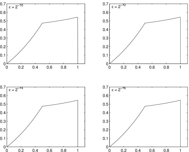
Figure 1. Graphs of the numerical solution of the first component $u_{1h}$ of the BVP (6.1)-(6.3) for various values of $\varepsilon$ with $N=512.$

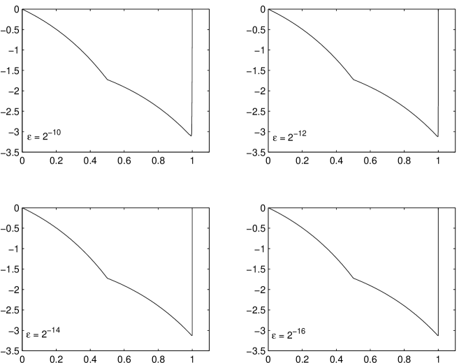
Figure 2. Graphs of the numerical solution of the second component $u_{2h}$ of the BVP (6.1)-(6.3) for various values of $\varepsilon$ with $N=512.$

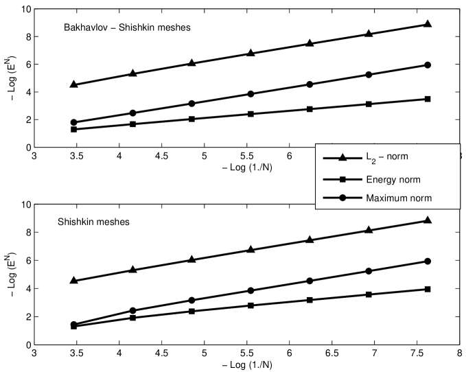
Figure 3. Plots of order of convergence for Example 6.1 and $\varepsilon=2^{-18}$ in various norms.

References

- [1] P. A. Farrell, A. F. Hegarty, J. J. H. Miller, E. O’Riordan, G. I. Shishkin, Robust computational techniques for boundary layers, Chapman Hall/ CRC, Boca Raton, 2000.
- [2] H-G. Roos, M. Stynes, L. Tobiska, Numerical methods for singularly perturbed differential equations, Volume 24 of Springer series in Computational Mathematics, Springer-Verlag, Berlin, 1996.
- [3] E.P. Doolan, J.J.H.Miller, W. H. A. Schilders, Uniform numerical methods for problems with initial and boundary layers, Boole, Dublin, 1980.
- [4] A. H. Nayfeh, Introduction to Perturbation Methods, Wiley, New York, 1981.
- [5] R. E. O’Malley, Singular perturbation methods for ordinary differential equations, Springer, New York, 1990.
- [6] H-G. Roos, Helena Zarin, The streamline-diffusion method for a convection-diffusion problem with a point source,J. Comp. Appl. Math.,Vol.10, No.4(2002) 275-289.
- [7] T. Lin, N. Madden, A finite element analysis of a coupled system of singularly perturbed reaction-diffusion equations, Appl. Math. Comput. 148(3)(2004)869-880.
- [8] N. Madden, M. Stynes, A uniformly convergent numerical method for a coupled system of two singularly perturbed linear reaction-diffusion problems, IMA. J. Numer. Anal.23(4)(2003)627-644.
- [9] H-G. Roos, T. Lin, Sufficient conditions for uniform convergence on layer-adapted grids, Computing 63 (1999) 27-45.
- [10] T. Lin, N. Madden, An improved error estimate for a system of coupled singularly perturbed reaction-diffusion equations, Comput. Methods Appl. Math. 3(2003)417-423.
- [11] Zhongdi Cen, Parameter-uniform finite difference scheme for a system of coupled singularly perturbed convection-diffusion equations, International Journal of Computer Mathematics, 82 (2005) 177-192.
- [12] S. Bellew, E. O’Riordan, A Parameter robust numerical method for a system of two singularly perturbed convection-diffusion equations, Journal of Applied Numerical Mathematrics, 51(2004) 171-186.
- [13] A. Tamilselvan, N. Ramanujam, A numerical method for singularly perturbed system of second order ordinary differential equations of convection-diffusion type with a discontinuous source term, Submitted for publication.