Enhanced X-ray Emission Coinciding with Giant Radio Pulses from the Crab Pulsar
Giant radio pulses (GRPs) are sporadic bursts emitted by some pulsars, lasting a few microseconds. GRPs are hundreds to thousands of times brighter than regular pulses from these sources. The only GRP-associated emission outside radio wavelengths is from the Crab Pulsar, where optical emission is enhanced by a few percent during GRPs. We observed the Crab Pulsar simultaneously at X-ray and radio wavelengths, finding enhancement of the X-ray emission by (a 5.4 detection) coinciding with GRPs. This implies that the total emitted energy from GRPs is tens to hundreds of times higher than previously known. We discuss the implications for the pulsar emission mechanism and extragalactic fast radio bursts.
Spinning neutron stars emit periodic radio pulses from their magnetospheres, which can be observed as a pulsar. The radio pulses are emitted by a coherent mechanism (?). Some pulsars also show optical, X-ray, and gamma-ray pulses, which are usually interpreted using incoherent emission mechanisms. Giant Radio Pulses (GRPs) are a form of sporadic pulsar emission with radio fluences at least an order of magnitude higher than those of regular pulses, of unknown origin (?, ?). GRPs have a power-law intensity distribution, unlike regular pulses which have log-normal or exponential intensity distributions (?).
GRPs are bright, sometimes exceeding a megajansky (MJy, ) for a few nano- to microseconds (?). This is sufficient to detect each GRP during a single stellar rotation. GRPs from young neutron stars have been proposed as the origin of fast radio bursts (FRBs), short-duration radio transients at cosmological distances (?, ?). A nearby counterpart has provided evidence for this association (?, ?) and for a connection between coherent and incoherent processes in the neutron star magnetosphere (?). Although GRPs are not the leading explanation for FRBs, the broad-band characteristics of GRPs provide information on coherent radio emission in neutron star magnetospheres, which may be relevant to FRBs.
GRPs have been detected from only a small fraction of pulsars (?, ?). The pulsar in the Crab Nebula, known as the Crab Pulsar (PSR B0531+21), was initially discovered by its GRPs (?). Regular periodic emission from the Crab Pulsar occurs from low frequency radio to high-energy gamma rays. At 2 GHz (S-band), the GRP emission occurs at two places: the main pulse (MP), and the inter-pulse (IP), with a separation of 0.4 cycles in phase. Sporadic GRPs occur both at the MP and IP of the average radio pulse, with each individual GRP lasting for a much narrower interval ( in phase) than the regular pulse.
Previous studies have searched for a correlation between radio giant pulses and higher energy emission [table S1 and the supplementary materials (?)]. The radio flux of GRPs is 2–3 orders of magnitude higher than regular pulses; such a large enhancement does not occur at other wavelengths. An enhancement of 3% ( significance) is known in the optical band (650–700 nm) (?) and independently confirmed (?). X-ray and gamma-ray observations have not detected any statistically significant correlations.
We searched for enhancement in X-rays during GRPs from the Crab Pulsar, using the Neutron star Interior Composition Explorer (NICER) X-ray observatory, mounted on the International Space Station (?). NICER has an effective collecting area of 1,900 cm2 at 1.5 keV, high time resolution (100 ns), and flexible scheduling. Since launch in 2017, we have monitored the Crab Pulsar with NICER for calibration and scientific purposes. The total average count rate of the Crab Pulsar and Nebula is counts s-1 in the 0.3–10 keV band ( counts per spin cycle), below NICER’s maximum throughput of counts s-1, and thus the data are nearly unaffected by pileup, dead-time, and data transfer losses. We also observed the Crab Pulsar with two radio telescopes in Japan: the 34 m radio telescope of the Kashima space technology center (?) and the 64 m radio dish of the Usuda deep space center, both operating at 2 GHz S-band [tables S2-S5 and figs. S1-S8; details are given in (?)].
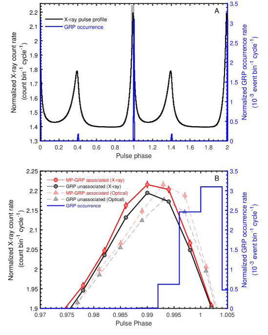
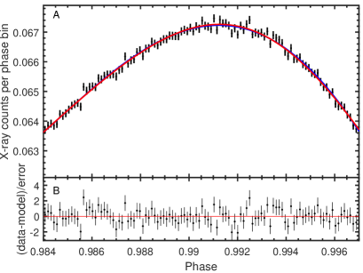
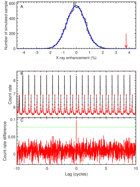
In 2017–2019, we coordinated 15 NICER observations concurrently with either the Usuda or Kashima observatories [tables S2, S6 and (?)]. We extracted a total of 126 ks of exposure with simultaneous radio and X-ray coverage (?). The arrival time of each X-ray photon was converted to barycentric dynamical time (TDB). Figure 1A shows the measured X-ray pulse profile in bins of 132 µs. The X-ray MP peak precedes the average radio profile by the rotation phase (300 µs), as previously reported (?). A constant component from the Crab Nebula ( counts s-1) was subtracted before the following analyses.
During the concurrent coverage, we detected and GRPs at the MP (hereafter referred to as MP-GRPs) and IP (hereafter IP-GRPs) phases at 0.9917 to 1.0083 and 1.3944 to 1.4111, respectively. The occurrence rates of MP-GRPs and IP-GRPs at S-band are 0.67% (24,851 cycles) and 0.047% (1,749 cycles), respectively, of the observed 3,731,830 pulsar rotations. Figure 1 shows the phase distribution of the GRPs. We defined our GRP samples as those pulses with signal-to-noise ratio exceeding 5.0, which corresponds to a fluence of Jy µs [fig. S8 (?)]. The occurrence phases and fractions of the MP- and IP-GRPs are consistent with past measurements (?, ?).
We combined the X-ray photons in three bins, corresponding to pulsar rotation cycles where MP-GRPs, IP-GRPs, or neither occurred. These are hereafter referred to as MP-GRP-associated, IP-GRP-associated and non-GRP-associated X-ray events, respectively. Figure 1B compares the MP-GRP-associated X-ray profile with the non-GRP-associated profile. The MP-GRP-associated X-ray profile shows an enhancement around the phase of the MP, with similar characteristics to that of the previously reported optical enhancement (?, ?). Within the pulse phase interval 0.985–0.997 [the same width as the optical measurement (?), taking into account the observed phase shift between the X-ray and optical bands (?)], the MP-GRP-associated X-ray profile shows an enhancement by 3.80.7% over the non-GRP-associated profile. We performed the same analysis for IP-GRP-associated X-rays, but did not find statistically significant results. We derived a 3 upper limit of the enhancement as 10% at 1.378-1.402 rotational phase (?). Hereafter we focus on the MP-GRP-associated case.
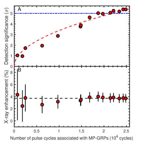
To evaluate the statistical significance of this enhancement, we generated synthetic X-ray samples that have no correlation with MP-GRPs, taking into account the look elsewhere effect (?). We randomly selected X-ray events with the same number of cycles as the MP-associated ones (24,826 cycles) from the non-GRP-associated sample. We repeatedly generated 1,000 synthetic control samples and made a histogram of simulated enhancements (?). This histogram follows the Gaussian distribution with a mean and standard deviation of % and 0.70%, respectively. Thus, the significance of the measured enhancement is 3.8% / 0.70% 5.4. Figure 2 shows the growth curves of detection significance and the X-ray enhancement rate as a function of the accumulated numbers of MP-GRP-associated cycles. The curves show a monotonic increase of the significance that follows the square-root of the number of the MP-GRP-associated cycles and a consistent X-ray enhancement rate. This detection is also confirmed by a lag analysis (?). We did not detect any spectral changes at the MP between the GRP-associated and the non-GRP-associated profiles except for the normalization increase corresponding to the enhancement (?).
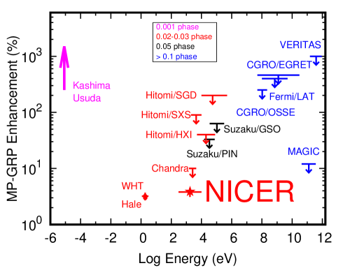
The total number of X-ray photons concurrent with radio observations in our analysis is counts, about three orders of magnitude larger than those in past X-ray studies [e.g., (?, ?)]. Figure 3 compares our detection of the X-ray enhancement of MP-GRPs with previous multiwavelength studies [table S1 (?)]. Our detection of a 3.8% X-ray enhancement is consistent with the upper limits of 10% obtained in previous studies and similar to the measured 3.2%% optical enhancement (?). The pulse phase where this X-ray excess appears, =0.985–0.997, is also consistent with the reported enhancement phase (=0.987–0.999) at optical wavelengths (?). This implies that the MP-GRP-associated higher-energy component extends from optical to X-rays without change of its pulse phase or a spectral cutoff compared to the average regular pulse. The X-ray flux of the regular pulsed emission ( ergs s-1 cm-2 in 0.3–10 keV) is 1000 and times higher than those of the optical [ ergs s-1 cm-2 at 5,500 Å, (?)] and regular radio pulses [ ergs s-1 cm-2 at 2 GHz, (?)], respectively. Assuming the same enhancement rate (4%) in both the optical and X-ray bands implies 1–2 order magnitude higher total energy (both flux and fluence) emitted from GRP-associated events than the value derived from the radio and optical data only. If the X-ray enhancement derived by averaging over µ s (Figure 1) consists of multiple short pulses similar to GRP pulses (a typical duration of µs for each GRP, evaluated as fluence divided by the individual peak flux), the peak X-ray flux could be much higher ( times) than the averaged enhancement flux.
These results constrain the GRP emission mechanism. The same degree of enhancements (4%) between the optical and X-rays indicates that the GRP-associated high-energy radiation has the same spectral energy distribution as that of regular pulses. Thus, the spectral energy distribution of GRP-emitting particles is similar to those of particles emitting regular pulses resulting from particle acceleration in the pulsar magnetosphere or a thin corrugated plasma flow at the equatorial plane (current sheet). The X-ray emission associated with GRPs implies that the radio emission efficiency is , consistent with the expectation from a magnetic reconnection model (?).
A proposed model of GRP high-energy radiation invokes a temporal increase in particle number density in the emitting region (?). The difference in enhancement between the radio (several orders of magnitude) and optical/X-ray bands (%) is then attributed to incoherent (X-ray and optical) emissions are proportional to the particle number, whilst coherent (radio) emission is proportional to the particle number squared [Supplementary Text in (?)]. Other proposed mechanisms are emission from high-energy particles in the plasma blobs (plasmoids) generated via magnetic reconnection (?) and from the resonant absorption of radio photons by X-ray emitting particles (?) (?).
Bright GRPs from young and energetic pulsars or magnetars have been proposed as low-energy analogues of FRBs (?) but this proposal has been disputed (?). The proposal relies on the unknown GRP radio emission efficiency relative to the spin-down luminosity. Even in the case of an extremely high efficiency (), the spin-down timescale for FRB sources are shorter than yrs (?, ?). If FRBs are accompanied by X-ray emission increases similar to Crab GRPs, the spin-down rate is enhanced by a factor of with . This would cause rapid radio flux decay, which is inconsistent with observations of such as the repeating FRB 121102 (?). Our results therefore disfavour the proposed connection between GRPs and the repeating FRBs.
References and Notes
- 1. D. B. Melrose, R. Yuen, Journal of Plasma Physics 82, 635820202 (2016).
- 2. H. S. Knight, M. Bailes, R. N. Manchester, S. M. Ord, B. A. Jacoby, Astrophys. J. 640, 941 (2006).
- 3. A. V. Bilous, M. A. McLaughlin, V. I. Kondratiev, S. M. Ransom, Astrophys. J. 749, 24 (2012).
- 4. W. A. Majid, C. J. Naudet, S. T. Lowe, T. B. H. Kuiper, Astrophys. J. 741, 53 (2011).
- 5. T. H. Hankins, J. A. Eilek, Astrophys. J. 670, 693 (2007).
- 6. D. R. Lorimer, M. Bailes, M. A. McLaughlin, D. J. Narkevic, F. Crawford, Science 318, 777 (2007).
- 7. J. M. Cordes, I. Wasserman, Mon. Not. R. Astron. Soc. 457, 232 (2016).
- 8. C. D. Bochenek, et al., Nature 587, 59 (2020).
- 9. CHIME/FRB Collaboration, et al., Nature 587, 54 (2020).
- 10. W. Lu, P. Kumar, B. Zhang, Mon. Not. R. Astron. Soc. 498, 1397 (2020).
- 11. R. N. Manchester, G. B. Hobbs, A. Teoh, M. Hobbs, Astron. J. 129, 1993 (2005).
- 12. T. Enoto, S. Kisaka, S. Shibata, Rep. Prog. Phys. 82, 106901 (2019).
- 13. D. H. Staelin, E. C. Reifenstein, III, Science 162, 1481 (1968).
- 14. Materials and methods are available as supplementary materials.
- 15. A. Shearer, et al., Science 301, 493 (2003).
- 16. M. J. Strader, et al., Astrophys. J. 779, L12 (2013).
- 17. K. C. Gendreau, et al., Space Telescopes and Instrumentation 2016: Ultraviolet to Gamma Ray (2016), vol. 9905 of Proc. SPIE., p. 99051H.
- 18. K. Takefuji, et al., Publ. Astron. Soc. Pac. 128, 084502 (2016).
- 19. A. Martin-Carrillo, et al., Astron. Astrophys. 545, A126 (2012).
- 20. R. Mikami, et al., Astrophys. J. 832, 212 (2016).
- 21. Hitomi Collaboration, et al., Publ. Astron. Soc. Jpn. 70, 15 (2018).
- 22. R. Bühler, R. Blandford, Rep. Prog. Phys. 77, 066901 (2014).
- 23. E. Gross, O. Vitells, European Physical Journal C 70, 525 (2010).
- 24. A. A. Abdo, et al., Astrophys. J. 208, 17 (2013).
- 25. A. V. Bilous, et al., Astron. Astrophys. 591, A134 (2016).
- 26. A. Philippov, D. A. Uzdensky, A. Spitkovsky, B. Cerutti, Astrophys. J. 876, L6 (2019).
- 27. M. Lyutikov, Mon. Not. R. Astron. Soc. 381, 1190 (2007).
- 28. A. K. Harding, J. V. Stern, J. Dyks, M. Frackowiak, Astrophys. J. 680, 1378 (2008).
- 29. M. Lyutikov, Astrophys. J. 838, L13 (2017).
- 30. S. Kisaka, T. Enoto, S. Shibata, Publ. Astron. Soc. Jpn. 69, L9 (2017).
- 31. M. Cruces, et al., Mon. Not. R. Astron. Soc. 500, 448 (2021).
- 32. C. P. Hu, Source code and GRP list for Crab GRP analysis, version 0.1, Zenodo (2021), https://doi.org/10.5281/zenodo.739138.
- 33. N. Kawai, R. Okayasu, Y. Sekimoto, American Institute of Physics Conference Series, M. Friedlander, N. Gehrels, D. J. Macomb, eds. (1993), vol. 280 of American Institute of Physics Conference Series, p. 213.
- 34. R. Mikami, ”Simultaneous multi-wavelength observation of giant radio pulses from the Crab pulsar”, Ph.D. thesis, The University of Tokyo, Tokyo (2016).
- 35. E. Argyle, G. Baird, J. Grindlay, H. Helmken, E. Omongain, Nuovo Cimento, Sezione B 24, 153 (1974).
- 36. S. C. Lundgren, et al., Astrophys. J. 453, 433 (1995).
- 37. P. V. Ramanamurthy, D. J. Thompson, Astrophys. J. 496, 863 (1998).
- 38. A. V. Bilous, et al., Astrophys. J. 728, 110 (2011).
- 39. M. B. Mickaliger, et al., Astrophys. J. 760, 64 (2012).
- 40. D. A. Moffett, T. H. Hankins, Astrophys. J. 468, 779 (1996).
- 41. T. H. Hankins, J. A. Eilek, G. Jones, Astrophys. J. 833, 47 (2016).
- 42. M. Tavani, et al., Science 331, 736 (2011).
- 43. E. Aliu, et al., Astrophys. J. 760, 136 (2012).
- 44. MAGIC Collaboration, et al., Astron. Astrophys. 634, A25 (2020).
- 45. T. H. Hankins, Astrophys. J. 169, 487 (1971).
- 46. D. R. Lorimer, M. Kramer, Handbook of Pulsar Astronomy, vol. 4 (Cambridge University Press, 2004).
- 47. Jodrell Bank Observatory, http://www.jb.man.ac.uk/pulsar/crab.html.
- 48. G. B. Hobbs, R. T. Edwards, R. N. Manchester, Mon. Not. R. Astron. Soc. 369, 655 (2006).
- 49. J. M. Cordes, N. D. R. Bhat, T. H. Hankins, M. A. McLaughlin, J. Kern, Astrophys. J. 612, 375 (2004).
- 50. N. D. R. Bhat, S. J. Tingay, H. S. Knight, Astrophys. J. 676, 1200 (2008).
- 51. B. Shaw, et al., Mon. Not. R. Astron. Soc. 478, 3832 (2018).
- 52. R. H. Dicke, Rev. Sci. Instrum. 17, 268 (1946).
- 53. V. I. Zhuravlev, et al., Astron. Rep. 55, 724 (2011).
- 54. J. F. Macías-Pérez, F. Mayet, J. Aumont, F. X. Désert, Astrophys. J. 711, 417 (2010).
- 55. T. L. Wilson, K. Rohlfs, S. Hüttemeister, Tools of Radio Astronomy (Springer, Berlin Heidelberg, 2013).
- 56. M. C. Miller, et al., Astrophys. J. 887, L24 (2019).
- 57. J. K. Blackburn, R. A. Shaw, H. E. Payne, J. J. E. Hayes, Heasarc, FTOOLS: A general package of software to manipulate FITS files (1999).
- 58. W. M. Folkner, J. G. Williams, D. H. Boggs, R. S. Park, P. Kuchynka, Interplanetary Network Progress Report 42, 1 (2014).
- 59. D. L. Kaplan, S. Chatterjee, B. M. Gaensler, J. Anderson, Astrophys. J. 677, 1201 (2008).
- 60. L. Kuiper, W. Hermsen, R. Walter, L. Foschini, Astron. Astrophys. 411, L31 (2003).
- 61. A. H. Rots, K. Jahoda, A. G. Lyne, Astrophys. J. 605, L129 (2004).
- 62. S. Molkov, E. Jourdain, J. P. Roques, Astrophys. J. 708, 403 (2010).
- 63. K. A. Arnaud, Astronomical Data Analysis Software and Systems V, G. H. Jacoby, J. Barnes, eds. (1996), vol. 101 of Astronomical Society of the Pacific Conference Series, p. 17.
- 64. M. Y. Ge, et al., Astrophys. J. 199, 32 (2012).
- 65. J. Wilms, A. Allen, R. McCray, Astrophys. J. 542, 914 (2000).
- 66. M. Morini, Mon. Not. R. Astron. Soc. 202, 495 (1983).
- 67. A. Saggion, Astron. Astrophys. 44, 285 (1975).
- 68. B. Cerutti, A. A. Philippov, Astron. Astrophys. 607, A134 (2017).
- 69. D. A. Uzdensky, A. Spitkovsky, Astrophys. J. 780, 3 (2014).
- 70. Y. E. Lyubarskii, Astron. Astrophys. 311, 172 (1996).
- 71. V. Trimble, Publ. Astron. Soc. Pac. 85, 579 (1973).
- 72. J. A. Eilek, T. H. Hankins, Journal of Plasma Physics 82, 635820302 (2016).
- 73. Y. E. Lyubarskii, S. A. Petrova, Astron. Astrophys. 337, 433 (1998).
- 74. S. A. Petrova, Mon. Not. R. Astron. Soc. 336, 774 (2002).
- 75. A. K. Harding, V. V. Usov, A. G. Muslimov, Astrophys. J. 622, 531 (2005).
- 76. B. Shaw, et al., The Astronomer’s Telegram 12957, 1 (2019).
- 77. NICER Background Estimator Tools, https://heasarc.gsfc.nasa.gov/docs/nicer/tools/nicer_bkg_est_tools.html.
- 78. S. Ansoldi, et al., Astron. Astrophys. 585, A133 (2016).
Acknowledgments
NICER analysis software and data calibration is provided by the NASA NICER mission and the Astrophysics Explorers Program. We thank Y. Terada and N. Kawai for suggestions on our analysis and manuscript. We thank the Usuda 64-m antenna operation support team in Space Tracking and Communication Center and ISAS, JAXA, and also E. Kawai and S. Hasegawa of the Space Time Standard Laboratory of the Kashima Space Technology Center of the National Institute of Information and Communications Technology (NICT) for supporting observations with the Kashima 34-m antenna. Funding: T.E.. T.T., H.M., K.A., M.H., S.S., S.J.T., and S.K., are supported by JSPS/MEXT KAKENHI grant numbers 15H00845, 15K05069,16H02198, 17H01116, 17K18270, 17K18776, 18H01245, 18H01246, and 18H04584, 19K14712. T.E. acknowledges Hakubi projects of Kyoto University and RIKEN. W.C.G.H. acknowledges support through grant 80NSSC20K0278 from NASA. C.H. was supported as the JSPS International Research Fellow (ID: P18318) and by the the Ministry of Science and Technology in Taiwan through grant MOST 109-2112-M-018-009-MY3. C.M. is supported by an appointment to the NASA Postdoctoral Program at the Marshall Space Flight Center, administered by Universities Space Research Association under contract with NASA. H.T. was supported by the discretionary expenses of the director of Institute of Space and Astronautical Science (ISAS), JAXA. W.A.M carried out research at the Jet Propulsion Laboratory, California Institute of Technology, under a contract with the NASA. Authors contributions: T.E. and T.T. led this radio-X-ray collaboration. T.T. and C.H. led the radio and X-ray timing analyses, respectively. S.G. performed the X-ray spectral analyses. S.K. led the theoretical discussion. P.S.R., T.O., Z.A., K.C.G., C.B.M., Y.S., S.K., S.B., and R.F. were responsible for NICER detector development, timing calibration, and observation planning. C.M., W.C.G.H., A.K.H., Z.W., W.A.M., T.G., G.K.J., K.A., S.S., N.L. and S.J.T. contributed the theoretical interpretation. Y.M., H.T., K.T., M.S., Y.Y., H.M., F.T., T.A., M.T., M.H., O.K., and T.O. were responsible for the radio observations and associated data analyses. N.L. contributed to summarize the previous studies. Competing Interests: We declare no competing interests. Data and materials availability: The NICER X-ray data and analysis softwares are available from the NASA HEASARC archive (https://heasarc.gsfc.nasa.gov/) and HEASoft (https://heasarc.gsfc.nasa.gov/docs/software/heasoft/), respectively. The observation IDs (ObsIDs) are listed in (?). The GRP event list and analysis source codes to reproduce the results of this article are available on Zenodo (?).
Supplementary Materials
-
•
Materials and Methods
-
•
Supplementary Text
-
•
Figures S1 to S20
-
•
Tables S1 to S7
-
•
References (33–78)
-
•
Movie S1
![[Uncaptioned image]](/html/2104.03492/assets/x4.png)
Materials and Methods
Previous searches for high-energy emission associated with GRPs
In this section, we review prior studies of GRPs in X-rays and gamma-rays from the Crab Pulsar. The upper limits derived from these observations are listed in Table S1.
X-rays
The search for a variation of the pulsed emission has been reported in several studies (?). One study (?) performed 5.4 hours of simultaneous observations of the Crab Pulsar with the Green Bank Telescope (GBT) at 1.5 GHz and the Chandra X-ray satellite at energies from 1.5 to 4.5 keV. They searched for an X-ray flux enhancement a) in the rotations during which GRPs occurred [for main pulse (MP) and interpulse (IP) GRPs separately], b) in the time windows around GRPs ranging from one up to 15 pulsar periods and c) during the GRPs that occurred simultaneously in both the X-ray and radio bands. In all three cases, no significant correlations were found, the results being compatible with 2 fluctuations.
A correlation search at hard X-rays from the Crab Pulsar was carried out with the Suzaku X-ray observatory simultaneously with the Kashima and Usuda radio telescopes (?). They found no significant flux increase in the 15–75 keV band (silicon PIN diodes of the Hard X-ray Detector; HXD-PIN) coincident with any of the GRPs and derived 95%-confidence upper limits of potential enhancements of 33% and 88% for the MP-GRPs and IP-GRPs, respectively. Similarly, they derived 95%-confidence upper limits of 63% and 193% in the 35–315 keV band (gadolinium silicate scintillators [Gd2SiO5(Ce)) of the HXD; HXD-GSO.
Correlation studies were carried out with the Hitomi X-ray satellite in an energy range from 2 to 300 keV and the Kashima radio telescope at 1.4 to 1.7 GHz (?). On the basis of the detection of 3,090 MP- and 260 IP-GRPs (1,000 MP- and 100 IP-GRPs were detected simultaneously) from about 2 ks of observations, searches for a) X-ray profile changes before and after GRP events and b) X-ray peak enhancements during GRP events were carried out. All examined variations were reported to be within 2 fluctuations of the X-ray fluxes at the pulse peaks.
Gamma-rays
A search for a correlation of GRPs with gamma-ray photons was carried out by (?). They observed the Crab pulsar simultaneously with the radio telescope of the Dominion Radio Astrophysical Observatory at 146 MHz and with the Whipple Imaging Air Cherenkov Telescope (IACT) at energies above 200 GeV for about 10 hours, and detected 300 GRPs. The time resolution of the observations was 200 µs, which enabled them to carry out correlation searches at time scales of one to five rotation periods of the Crab pulsar. No statistically significant enhancement was found.
Correlation searches of GRPs with gamma-ray photons have been carried out predominantly with spacecraft. Simultaneous observations with the 43 m Green Bank radio telescope at 0.8 and 1.4 GHz and the Oriented Scintillation Spectrometer Experiment (OSSE) on the Compton Gamma-Ray Observatory (CGRO) in an energy range from 50 to 220 keV resulted in a collection of about 3,600 GRPs. No increases of the gamma-ray flux by more than a factor of 2.5 were detected (?).
Further correlation searches were carried out with the GBT at 0.80, 0.81, and 1.33 GHz and with the Energetic Gamma Ray Experiment Telescope (EGRET) onboard the CGRO at energies higher than 50 MeV (?). On timescales ranging from 6 to 30 pulsar rotations, no enhancement of the gamma-ray flux at energies above 50 MeV was found.
Searches for correlations between GRPs and gamma-ray photons were also carried out with 10 h-long simultaneous observations of Fermi Large Area Telescope (Fermi-LAT) and GBT (?, ?), targeting a specific class of GRPs that occur at the phase ranges of the High Frequency Interpulse Component, HFIP (?, ?), as predicted by a theoretical model (?). They observed GRPs at 8.9 GHz and 77 gamma-ray photons with energies between 100 MeV and 5 GeV and searched for a correlation between the occurrence frequency of GRPs and single gamma-ray photons, as well as changes of gamma-ray flux during and around the period of each GRP. No significant changes in the GRP generation rate were detected in time windows ranging from 10 to 120 seconds, with a 95% upper limit for a gamma-ray flux enhancement in a pulsed phase emission window around the observed GRPs of four times the average pulsed gamma-ray flux of the pulsar.
Studies using Fermi-LAT (?) used 107 h of simultaneous observations at 0.33 and 1.2 GHz with the 43 m radio telescope in Green Bank, where the energy of the gamma-ray data ranged between 0.1 and 100 GeV. They examined correlations and anti-correlations of 92,022 detected (MP and IP) GRPs with regard to their 393 gamma-ray photons (at time lags of rotation periods), collected from the period before and after the Crab Nebula flare, a sudden increase of unpulsed gamma-ray flux from the nebula observed in October 2007 and September 2010 (?). They determined the largest deviations from the mean of random correlations to be 2.4 and 2.1 for anti-correlated post-flare 1.2 GHz MP GRPs and correlated pre-flare 1.2 GHz IP GRPs, respectively, at a time lag of 20,000 rotation periods. They concluded that these were not statistically significant.
Correlation searches were carried out with the Very Energetic Radiation Imaging Telescope Array System (VERITAS) at very high energy (VHE) gamma-rays above 150 GeV and the GBT at a frequency of 8.9 GHz (?) and investigated HFIP GRPs. Using 15,366 GRPs and 30,093 gamma-ray photons, they searched the detected MP and IP GRPs for an enhancement of pulsed gamma-ray emission in eight-time windows with durations from one up to 2,182 rotation periods at three locations with regard to a GRP to account for leading, lagged and concurrent correlations. They reported upper limits of the gamma-ray flux of the Crab Pulsar during HFIP GRPs that were detected simultaneously with the radio data to be five to ten times the average flux and two to three times the average gamma-ray flux on time scales of about eight seconds around HFIP GRPs.
A study covering energies above 60 GeV, was carried out using the Major Atmospheric Gamma-ray Imaging Cherenkov telescopes (MAGIC) and the Effelsberg radio telescope and the Westerbork Synthesis Radio Telescope (WSRT) at 1.3 GHz (?). They observed 99,444 GRPs and 433 gamma-ray photons from 16 hours of overlapping observations, and performed correlation searches of MP and IP GRPs at time windows with durations ranging from 1/9 to 2,187 rotation periods and three different locations with respect to each GRP, following the approach of (?). The authors reported no statistically significant correlation between GRPs and gamma-ray photons for time windows of 1/9, 1/3, 1 and 3 rotation periods, reporting upper limits of 12% to 2,900% on the flux increase of the pulsed gamma-ray flux during a radio GRP.
Radio data and analysis
Radio observations
Radio observations of the Crab Pulsar were performed using radio telescopes at Usuda and Kashima (Table S2) in the S and X bands for right hand circular polarization with eight channels in total: four S-band channels (ch0–3: 2,194–2,226 MHz, 2,226–2,258 MHz, 2,258–2,290 MHz, and 2,290–2,322 MHz) and four X-band channels (ch4–7: 8,374–8,406 MHz, 8,406–8,438 MHz, 8,438–8,470 MHz, and 8,470–8,502 MHz) and a total data rate of 2.048 Gbits/s (= 8 channels 4 bits 64M samples/s). We only report the S-band data because there are not enough GRPs in the X band data. While we analyze all four S-band channels of the Usuda data, we only consider three S-band channels (ch0, ch2, and ch3) of the Kashima data as one channel (ch1) was severely affected by radio frequency interference (RFI). In Table S3, all observing sessions are tabulated with the parameters used in the analysis.
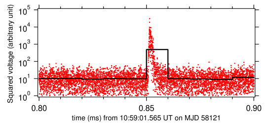
De-dispersion and an example of GRP
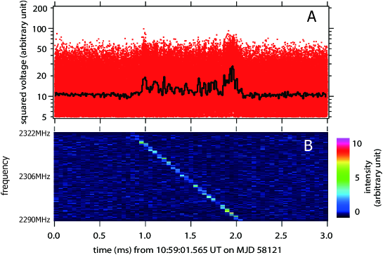
In this subsection, we present example data obtained using the Usuda radio telescope on MJD 58121 (session 4). Fig. S1A shows the squared raw-antenna voltages in channel 3, , for a 3 ms duration, along with their 10 µs averages. A dynamic spectrum (Fig. S1B) shows a down-tone chirp signal, which indicates arrival of a pulse with a frequency dispersion, or a group delay, caused by interstellar free electrons. This frequency dispersion can be removed by a coherent de-dispersion process (?, ?), which is described as,
| (S1) |
where is antenna voltages after de-dispersion and is the complex conjugate of a transfer function with a base frequency (2,322 MHz for ch3) and an offset ,
| (S2) |
where MHz pc-1 cm3 (, , and are electron charge, electron mass, and speed of light, respectively) and DM56.7548 pc cm-3. In Fig. S2, squared values for a 0.1 ms duration (i.e. zooming into part of Fig. S1A after de-dispersion) indicate a pulse with a few µs duration (this pulse is identified as an MP GRP in our subsequent analysis; see Spin number, phase, and GRP identification subsection). With a time constant µs, we take the average
| (S3) |
for binned times , where is the start time of the observing session. The resultant is overlaid in Fig. S2.
Initial data processing
We de-disperse data (in each channel ) from all observing sessions in the same way as described in the previous subsection and obtain for defined for each session. Since DM of the Crab Pulsar shows time variations with time scale as short as several days, DM should be evaluated for each session. We determine DM iteratively so that the sub-microsecond structures of GRPs in all frequency channels are aligned to each other after the de-dispersion procedure. For the initial trial value of a DM in each iteration, we use values from the Jodrell Bank ephemeris (?). The estimated uncertainty of DM is 0.001 , which corresponds to the uncertainty of the pulse arrival time 0.76 µs or that of the spin phase .
From we make incoherent summations,
| (S4) |
where runs over the available channels (four channels for Usuda and three channels for Kashima) and is a group delay time between channels and 3 (). For , is linearly interpolated from the values of at .
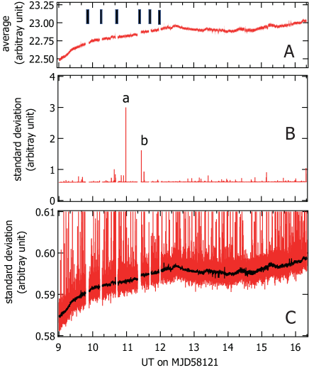
From of µs duration, we calculate 1 s averages and standard deviations , where are integer seconds, i.e.,
| (S5) |
As an example, Fig. S3 shows and from 9:00:00 UT to 16:20:00 UT of session 4. In panel A, shows a gradual variation (2%), which is caused by the gain drift of the receiving system. In panel B, there are spikes of , the largest of which (marked a) corresponds to the MP GRP shown in Fig. S2. This short ( µs) GRP boosted the 1 s standard deviation by a factor of 5. Another spike (marked b) corresponds to an MP GRP at 11:26:30 UT. In panel C, which shows with an enlarged vertical scale, there are numerous spikes, which are all identified as MP/IP GRPs (see Spin number, phase, and GRP identification subsection). To remove these spikes for the following signal-to-noise analysis, we define the standard deviation not affected by GRPs as , which is approximated as (a black line in Panel C). The signal to noise ratio, SNR at , is then defined as,
| (S6) |
Two GRPs corresponding to the spikes a and b in Fig. S3 are found to have peak signal-to-noise ratios of 1712.7 and 799.9, respectively.
Time-domain RFI rejection
To eliminate RFI from both Usuda and Kashima data in the time domain, we calculate summations of the squared raw antenna voltages (without de-dispersion) directly from , i.e.,
| (S7) |
where runs over the channels used. We calculate its average [] and standard deviation [] for each 1 s interval. If exceeds , we reject the data for and regard it as being affected by RFI. After this procedure, we visually inspect all remaining data and further reject intervals where RFIs appear to still remain. We find 99.3% and 94.0% of Usuda and Kashima data, respectively, are free from RFI.
Spin number, phase, and GRP identification
We use the pulsar timing package TEMPO2 (?) to convert to the Solar System barycenter time (TDB) . From , we calculate turn , daily sequential spin number , and spin phase according to
| (S8) |
where is the initial phase, and are the spin frequency and its time derivative, respectively, all of which are determined at =00:00:00 TDB of the day of the observing session with the interpolated values of the Jodrell Bank monthly ephemeris (?). The values of and are tabulated in Table S3. The planetary ephemeris used by the Jodrell Bank observatory (DE200) differs from that used by the NICER data analysis (DE430). We checked how the parameters , , and appearing in equation (S8) depend on the choices of DE200/DE430 and found that only the dependence of should be taken into account and that those of and are negligible for estimating . The uncertainty of is at most (Table S3), which is 2% of the accumulation bin size for GRP and X-ray photons so it has a negligible effect on our analysis. The mathematical function for a real number returns the integer satisfying . As a result, the range of the phase is guaranteed to be , where the peak of the average main pulse is placed at phase .
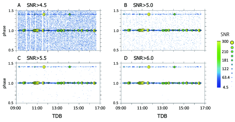
Fig. S4 shows diagrams of time versus phase for of observing session 4 with four different lower threshold values of the signal to noise ratio SNRthr. We find two data clusters at phases of 1 and 1.406. Data-points from phase ranges 0.9917–1.0083 and 1.3944–1.4111 are categorized as the MP and IP GRP candidates, respectively [figure 4 of (?)]. If multiple MP/IP GRP candidates at the same are found, we choose the one with the maximum SNR as representing the MP/IP GRP at this . Outside the MP and IP phase ranges, there are background data-points, whose distribution does not depend on and varies from dense (panel A) to sparse (panel D) depending on SNRthr. By assuming homogeneity over , we calculate the pseudo event density per unit , , and obtain the expected value of the false GRP number, , where is a phase width (0.0167 for both MP GRP and IP GRP). If we observe candidates for MP GRP with SNRSNRthr, the expected value of a true MP GRP number is . Let and be the numbers defined above for session . False-positive MP GRP rates of Usuda and Kashima data are calculated as
| (S9) |
respectively, where and . Similarly, false-positive IP GRP rates of Usuda and Kashima data are calculated. Table S4 lists the numbers of GRP candidate and false-positive GRP rates, both of which are decreasing functions of SNRthr. Because the sensitivity of the Kashima observatory is 55% that of the Usuda observatory, the false GRP rates for Kashima are higher than those for Usuda. There are two competing factors; it is desirable (1) to have as much observed numbers of GRP candidates and (2) to reduce false GRP rates. Balancing these two factors, we choose SNRthr=5 for the following analysis.
If a GRP occurs at around the time between and , its contribution to the squared voltage is split into and , and the peak intensity is artificially lowered. To compensate for this effect, we further perform a half-shifted-bin procedure (see section A.1.4 of (?)). In the worst case, SNR at the peak of a GRP becomes lower than SNRthr, and accordingly this GRP is miscounted. This type of miscount is handled with this procedure.
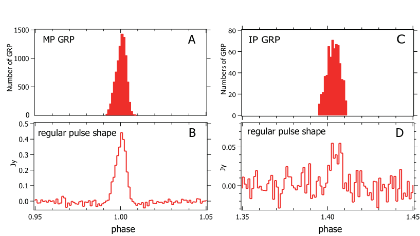
GRP and regular pulse shapes
The phase ranges of GRPs of the Crab Pulsar coincide with those of the regular pulses [e.g., (?, ?)]. We confirmed this property by comparing the number of GRPs and regular pulse shapes for all observing sessions. An example (from observing session 4) is shown in Figs. S5A and B for MP GRPs and in C and D for IP GRPs. We find that the occurrence of GRPs is limited to the phase ranges of the corresponding regular pulses.
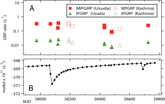
Temporal variations of the GRP detection rate
Table S5 summarizes our GRP identification for all observing sessions. The temporal variations of the GRP detection rates are usually interpreted as an effect of interstellar scintillation (?). These observing sessions include the epoch of a large glitch in the Crab Pulsar rotation rate (?). We checked whether this glitch affected the GRP rate. In Fig. S6, we compare the variations of the GRP rate with variations of the spin rate change () taken from the Jodrell Bank ephemeris (?). We find no change in the GRP rates with respect to .
Flux density and fluence
Because observations did not involve the use of switching noise diodes for absolute flux calibration, we estimate flux density using the radiometer equation (?, ?)
| (S10) |
where SEFD (system equivalent flux density) and (effective band width) are tabulated in Table S2. is the integration time (10 µs), and is the number of polarizations observed (1). is the flux density of the Crab Nebula, which depends on the antenna aperture and the observation epoch (MJD). Following (?) (see also The flux density of the Crab Nebula subsection), we calculated Jy for Usuda and Jy for Kashima, where is a decaying factor of the total nebula emission. We included the decaying factor for completeness. However, this factor gives negligible changes of and throughout observing sessions 1-15.
Our GRP selection criterion of SNR5 corresponds to 109 Jy for Usuda and 199 Jy for Kashima on MJD57974. We calculate the fluence of a GRP from according to
| (S11) |
where runs over time intervals during which we judge that there is an enhancement of SNR() relating to this GRP. For example, the MP GRP shown in Fig. S1 has a peak intensity of 3.7 Jy and fluence of 4.1 Jy µs.
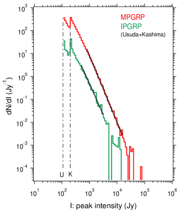
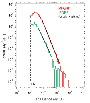
Figs. S7 and S8 show the differential flux and fluence histograms of the MP GRPs and IP GRPs for the combined data (UsudaKashima). The middle part of the intensity histograms, specifically in intensity ranges – Jy and – Jy for MP and IP GRPs, respectively, are found to have power-law dependence on the intensity with indices of and (Fig. S7). Similarly, the middle part of the fluence histograms show power-law dependence (Fig. S8): fluence ranges of –µs and –µs, respectively, with indices of and . The spectral index for the MP GRP fluences is consistent with previous observations (?) in the 2 GHz band. These authors reported the power-law index of for a cumulative fluence histogram of MP GRPs in a fluence range of –µs, which corresponds to the index 3.0 for the corresponding differential fluence histogram. They also observed an index change from 2.0 to 1.1 at a cumulated flux range below µs, where our result is inconclusive because it is close to our detection limit.
The flux density of the Crab Nebula
With the angular distance from the center of Crab Nebula , the spatial intensity distribution of the Crab Nebula is approximated as (?)
| (S12) |
where size is in units of 3 arcmin. The coefficient is normalized such that
| (S13) |
where the total flux density of the Crab Nebula at frequency is a decaying function at epoch (year or MJD) (?),
| (S14) |
An antenna with a diameter at an observing wavelength detects the Crab Nebula with a flux density
| (S15) |
where is the antenna pattern function
| (S16) |
with beam size (?). At the center of our observing frequency GHz ( cm), we calculate for Usuda ( m) and for Kashima ( m) from equation (S15) and find
| (S17) |
where is the decaying factor from the second line of equation (S14).
X-ray data and analysis
Data reduction and verification
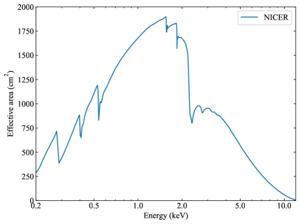
The X-ray timing instrument of NICER (?, ?) consists of co-aligned X-ray concentrators coupled with silicon drift detectors at its focal plane. The NICER detectors have a time resolution of ns, corresponding to cycles of the spin period of the Crab Pulsar. It has 56 focal-plane modules, four of which were inactive during the observations. Figure S9 shows the NICER’s effective collecting area as a function of energy around 1.5 keV.
We used 15 NICER observations carried out in 2017–2019. Table S6 summarizes the observation log. We performed basic data analysis with NICERDAS version 6 in HEAsoft 6.26 (?) and NICER calibration database version 20190516. We created level-2 cleaned event files by applying nicerl2 command to the unfiltered data, setting the underonly_range="0-500" (default value: 200) and overonly_range="0-10" (default value: 1) to maximize the available exposure time. To correct the photon arrival times to the barycenter of the Solar System, we used the barycorr command, adopting the coordinates of Crab of R.A.=83.633218 and Decl.=22.014464 (J2000 equinox) and the Jet Propulsion Laboratory Solar System development ephemeris DE430 (?). We refer to the spin ephemerides listed in Table S3 at the radio data and analysis section. The proper motion of the Crab Pulsar is negligible (?). We created Good Time Intervals (GTIs) during which Crab was simultaneously observed with NICER and radio telescopes. All the X-ray photons that were not covered by the merged GTI were excluded in this analysis.
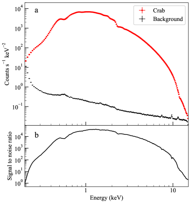
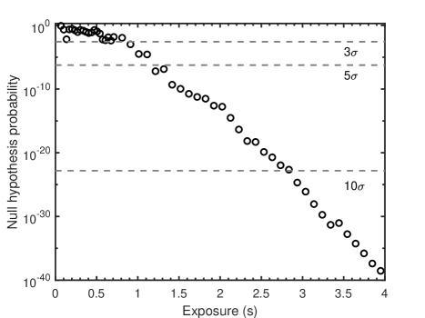
Figure S10a shows the X-ray spectrum of the Crab Pulsar plus the surrounding nebula obtained with NICER. Compared with the source spectrum, the background is negligible except for the lowest energy band. We found that the signal-to-noise ratio was higher than 100 in 0.3–10 keV. Therefore, we selected X-ray photons in the energy range of 0.3–10 keV to maximize the signal to noise ratio. In the 0.3–10 keV band, the background contamination is 1% of the source intensity. Figure S11 shows the detection significance with NICER of a pulsation from the Crab Pulsar as a function of the exposure time. The Crab pulsation is detectable at an exposure of 1 sec (30 pulse rotations) or longer. Movie S1 shows how the accumulated Crab pulse profile evolves as the NICER exposure increases.
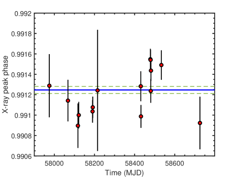
Figure S12 shows the X-ray pulse profile around the MP of the Crab Pulsar obtained by stacking all the NICER data. We folded the light curve with 8192 phase bins, and decompose the profile with the Fourier transform. The pulse peak is measured at 0.991250.00004, which is estimated by the Fourier series with 100 harmonics (?). We also fitted the pulse profile near the X-ray peak with a 4-th order polynomial function, which gave consistent results to the Fourier-filtered pulse profile. This corresponds to a radio delay of 304 µs compared to the X-rays; this delay is consistent with the previously reported ranges [figure 2 of (?), figure 4 of (?), and (?)]. The stability of the MP peak is shown in Figure S13. The uncertainties of the peak determination and phase jump of the NICER monitoring are smaller than those obtained in previous studies.
Search for X-ray enhancement coinciding with GRPs
We assigned a pulse phase to each X-ray photon on the basis of the radio ephemeris in Table S3, and classified them into three categories: MP-GRP associated, IP-GRP associated, and GRP unassociated events. Given that the MP-GRP arrival phases were distributed between pulse phases 0.992 and 1.008, we define an MP-GRP associated cycle as one where the main peak encompasses MP-GRPs. We calculated the pulsed emission, using the count rate between phases 0.985 and 0.997. This phase interval, 0.012 spin cycles centered at the X-ray peak, is selected for comparison with previous optical measurements (?, ?). The off-pulsed emission between phases 0.7 and 0.8, which included emission from the pulsar wind nebula and background, was subtracted from the light curve. The enhancement was calculated from the difference between the averaged pulsed emission from the MP-GRP associated and GRP-unassociated cycles.
The detection significance of the enhancement was estimated with Monte Carlo simulations (see Figure S14a). In each simulation run, we randomly choose 24851 cycles, which contains the same amount as that of the MP-GRP-associated one, from the non-GRP-associated sample. Then, we treated these selected cycles as fake MP-GRP-associated cycle and calculated the enhancement as using the same way as in the previous paragraph. We repeated this procedure times. The mean value of all is expected to be close to zero because the sample is chosen from non-GRP-associated cycles. The standard deviation of the enhancement of the simulated data sets represent 1 significance level if the observed enhancement is caused by the statistical fluctuation. The detection significance is defined as
| (S18) |
where is the observed enhancement from MP-GRP associated cycles. The resulting X-ray enhancement is described in the main text.
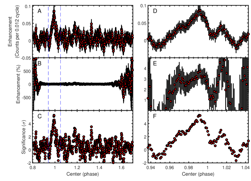
In the main text, we fixed the phase width at 0.012 and center at 0.991 to compare our X-ray results with the previous reports at the optical wavelength (?). Figure S15 shows the pulse phase in the MP during which the X-ray enhancement appeared as a function of the pulse phase center. The constant enhancement stays at % level in the range although the significance is lower than 5. This suggests that the X-ray enhancement occurs at a wider phase range than the range () found in the optical.
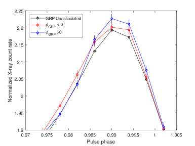
We further divided MP-GRPs into two groups with and , and tested whether the associated X-ray enhancements are GRP-phase-dependent. Following the same procedure described above, the X-ray pulse profiles associated with these two groups of MP-GRPs are shown in Figure S16. To test whether the enhancement is GRP-phase-dependent, we enlarged the phase range of calculation to 0.975–1.000. We found an enhancement of % with a significance of 3.5 for and an enhancement of % with a significance of 4.5 for . The difference in the enhancements of these two groups is not statistically significant. We also divided MP-GRPs into bright and faint groups according to their radio fluxes, but did not find a difference between the X-ray enhancement associated with bright and faint MP-GRPs.
Finally, we searched for enhancement of IP-GRP associated cycles. Following above procedures, the pulse profiles with GRP unassociated cycles and IP-GRP associated cycles near the IP are shown in Figure 1 Compared to Figure 1, the uncertainties of IP-GRP associated pulse profile are large and we could not observe statistically significant enhancement and estimated a 3 upper limit of the enhancement of %.
Lag analysis
We also performed a lag analysis by shifting the pulse number of X-ray events to search for potential correlations around the MP. The results of this analysis are shown in Figure S14b for pulse lags of cycles. We found no statistically significant enhancement ( sigma) around the lag over 10 cycles and thus confirmed our detection.
Spectral analysis for the MP-GRP-associated X-rays
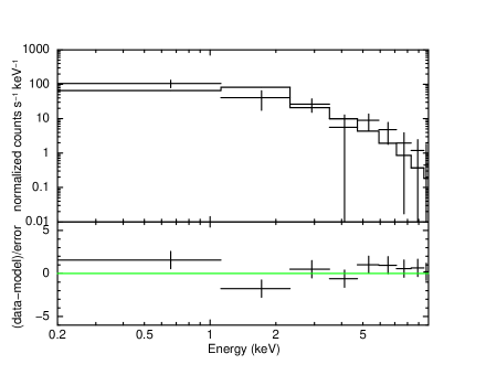
For the spectral analysis, we extracted the MP-GRP-associated and non-GRP-associated spectra as described in the main text. Events were selected within the phase interval (see Search for X-ray enhancement coinciding with GRPs subsection , i.e., with the phase width of ). For the background spectra, we extracted events from the phase interval , i.e., with as described in the main text. The exposure times for the MP-GRP-associated and non-GRP-associated spectra were calculated by taking the number of unique rotations encompassing the extracted MP-GRP-associated and non-GRP-associated events, respectively, then multiplying by the corresponding spin frequencies and by . This spectral extraction procedure was performed for individual ObsIDs. The individual spectra were then combined with the HEASoft mathpha tool (?), which merges source and background spectra. The source spectra are binned so that each spectral bin has at least 50 photons. We used xspec version 12.11.1 (?) for the spectral analyses of the combined MP-GRP-associated and non-GRP-associated spectra. We used the response matrix file (“nixtiref20170601v002.rmf”) and auxiliary response file (“nixtiaveonaxis20170601v004.arf”) released on July 22, 2020. We included 0.5% systematic uncertainty into the Non-MP-associated spectrum to allow for the uncertain accuracy of the detector response, which is known to be more pronounced for brighter objects.
The spectral model employed (tbfeologpar) was a log-parabola-shaped power-law (logpar) with an energy-dependent index (?) convolved with the absorption with letting the oxygen and iron abundances free (tbfeo) (?). Only the absorption parameters, the absorption column density and abundances for oxygen and iron, were tied between the MP-GRP-associated and non-GRP-associated spectra — the other model parameters for the two spectra were free parameters. We used the 0.2–10.0 keV range. The logpar model is defined by the X-ray flux (photons keV-1 cm-2 s-1) as a function of an X-ray energy as
| (S19) |
where , , and (photons keV-1 cm-2 s-1) are the parameters to be determined, and keV. Table S7 lists the best-fitting parameters for this model with 1-confidence uncertainties. The spectral parameters and of the two spectra were consistent within confidence. However, the 0.2-12 keV flux of the MP-GRP-associated spectrum, erg s-1 cm-2, was % higher than that of the non-GRP-associated spectrum, erg s-1 cm-2. If we allow only the normalization parameters free with fixing the other parameters, the 0.2–12 keV flux is erg s-1 cm-2 and erg s-1 cm-2 for the MP-GRP-associated and non-GRP-associated spectra, respectively. This corresponds with the enhancement at %, statistically consistent with the enhancement detected from the X-ray pulse profile in the main text.
We also investigated the cumulative distributions of the MP-GRP-associated and non-GRP-associated counts as a function of the instrument channel (i.e., free of uncertainty of the instrumental response). A Kolmogorov–Smirnov test on the exposure-scaled cumulative distributions demonstrates that both spectra follow the same count distribution, i.e., that they have the same spectral shape. This corroborates the finding of the spectral analyses above.
We extracted the net enhanced X-ray spectrum using the Non-GRP-associated data as background subtracted from the MP-GRP-associated spectrum. Due to the low statistics of this differential spectrum, we can not determine the absorption parameters. Using the same tbfeo model with the parameters fixed at the values shown in Table S7, the incident continuum is approximated (/d.o.f.=8.89/7) by a single power-law model with photon index and an absorbed 0.2-12 keV flux of erg s-1 cm-2, which is consistent with the differential flux estimated from Table S7. This is shown in Figure S18. This differential spectrum can be also approximated by the tbfeologpar model with the same (fixed) and values (/dof=9.74/8) only by changing its normalization. Thus, we can not statistically distinguish the MP-GRP-associated spectral shape from that of the regular pulses.
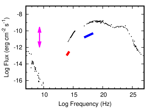
Figure S19 shows the broad-band spectral energy distribution of the flux enhancement of the Crab Pulsar during an MP-GRP. The X-ray enhancement was 3.8% of the persistent flux and showed no spectral change from the persistent emission.
Supplementary Text
Theoretical models for the X-ray enhancement during GRPs
Simple emission model from bunching particles
One simple interpretation of the radio and X-ray enhancements is a temporary increase of particle numbers in the emitting region. Only a small fraction of the X-ray emitting volume would be linked to the radio emitting region, which is common for both regular pulses and GRPs. This is supported by the narrow phase where the X-ray enhancement is detected (Figure 1), although the estimate of the actual volume of the emission would not be simple due to the caustic nature of the emitting region (i.e., emission originating at different regions in the magnetosphere being piled-up in phase, (?)). If coherent radio emission comes from particle bunches, the flux for a fixed number of bunches is proportional to the square of the particle density (e.g., (?)). Then a density increase of 16 times in the radio emitting volume leads to the typical flux ratio of GRP to regular radio pulses of . On the other hand, the enhancement of the X-ray flux with the emitting volume is . This suggests the volume fraction of the radio emitting region .
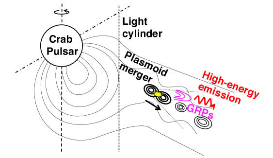
Magnetic reconnection model
We estimate the X-ray luminosity of GRP-emitting plasmoids on the basis of a reconnection model (?). We show a schematic picture of the model in Figure S20. In this model, a GRP is produced by collisions of multiple plasmoids in the current sheet beyond the light cylinder. Because the current sheet is unstable to plasmoid instability, the sheet is fragmented into a dynamical chain of plasmoids due to the magnetic reconnection [e.g., (?)]. A collision of plasmoids ejects fast magnetosonic waves, which escape from the plasma as electromagnetic radio waves. Considering cross-layer pressure balance and energy balance between heating by the magnetic energy dissipation and synchrotron cooling, the plasma density , thermal Lorentz factor , and current sheet thickness in the comoving frame are estimated to be cm-3, , and cm, respectively, for the magnetic field G at the light cylinder of the Crab Pulsar (?). Numerical simulations of the reconnection process (?) show that the typical size of a plasmoid is times larger than the thickness of the current sheet. As a result, the amount of magnetic energy released in an individual plasmoid collision is
| (S20) | |||||
where is the typical size of a plasmoid. Assuming that a fraction () of the released magnetic energy of a plasmoid is converted to radio emission (?) and that the bulk Lorentz factor of the plasma flow in the current sheet is (e.g., (?)), the observed flux density of an individual plasmoid merger event is expected to be
| (S21) | |||||
where kpc is the distance to the Crab Pulsar (?). Given that a large number of plasmoids would merge near the light cylinder of the Crab Pulsar due to tearing instability (?), multiple nanoshots may form a single GRP (e.g., (?)). In our observations, the typical duration of a GRP is s and the fluxes of most of the detected GRPs are close to the observation threshold value of Jy at 2 GHz (see the power-law distribution in Figure S6). Then, the number of the merging plasmoids observed in a GRP is estimated to be
| (S22) | |||||
The GRP-emitting plasmoids could emit synchrotron radiation in X-ray. Heating in the current sheet may be highly variable. A large fraction of particles has a Lorentz factor lower than the average value of . We assume that there is a fraction of low-energy electrons, which emit synchrotron radiation with the characteristic energy keV, corresponding to the Lorentz factor , in the GRP-emitting plasmoid. Then the synchrotron luminosity of a group of the multiple plasmoids which emit a single GRP is calculated to be
| (S23) | |||||
This luminosity corresponds to % of the average X-ray luminosity of the Crab Pulsar, which indicates that the observed radio and X-ray enhancements can be explained by the emission from plasmoids in the reconnecting current sheet beyond the light cylinder.
Radio absorption model
An alternative model for the X-ray flux enhancement correlated with a GRP is the cyclotron resonant absorption of radio photons by the synchrotron-emitting particles (?). In this model, relativistic particles maintain their pitch angles by absorbing radio photons that are in the cyclotron resonance in their rest frame. The power for the X-ray emission comes from the energy of the particles with radio photons acting as catalysts, providing the relativistic particles with a certain pitch angle so that they radiate synchrotron emission. The particles start out with very small pitch angles. When they begin absorbing the radio emission, their perpendicular momenta increase stochastically until they reach high Landau states, where their losses in the perpendicular momenta and increases in the pitch angles from absorption balance out. The resonant condition will occur in the outer magnetosphere near and beyond the light cylinder for the Crab Pulsar (?). The X-ray synchrotron flux should, therefore, depend on the radio flux that can be absorbed. Some of the radio emission in the direction of the observer may be absorbed, and the magnitude of the absorption optical depth is discussed elsewhere (?).
We estimate the expected amount of the increase of the X-ray flux from the increase of the radio flux during a GRP. Assuming that the momentum of a particle perpendicular to the magnetic field has reached an equilibrium between absorption and radiation losses [ (?), their equations (29) and (30)], we have the flux of synchrotron radiation
| (S24) |
where is the radio flux density. If the GRP flux is, on average, 100 times the regular radio flux, then the model would predict that the total synchrotron flux would increase by a factor of . However, the X-ray flux in the NICER band makes up only a fraction of the total Crab synchrotron flux, which extends from UV to gamma rays, and hence the expected flux increase in the NICER band would be much smaller. The model predicts an enhancement of the synchrotron component in the other energy bands as well and most of the power in the Crab spectrum lie between 50 keV and 1 MeV. No significant constraints on the enhancement in the MeV band have been reported.
| Band | Observatory | MP | IP | Ref. |
|---|---|---|---|---|
| Optical | William Herschel Telescope | 3% () | 2.5% () | (?) |
| (600-750 nm) | (WHT) | |||
| Optical | Hale Telescope | 3.2% (7.2) | 2.8%(3.5) | (?) |
| (1.1-3.1 eV) | ||||
| Soft X-ray | NICER | 3.8% (5.4) | 10% (3) | This work |
| (0.3–10 keV) | ||||
| Soft X-ray | Chandra | 10% (2) | 30% (2) | (?) |
| (1.5–4.5 keV) | ||||
| X-ray | Hitomi | 25% (3) | 110% (3) | (?) |
| (2–300 keV) | ||||
| Hard X-ray | Suzaku / HXD-PIN | 33% (2) | 88% (2) | (?) |
| (15–75 keV) | ||||
| Hard X-ray | Suzaku / HXD-GSO | 63% (2) | 193% (2) | (?) |
| (35–315 keV) | ||||
| Hard X-rays | OSSE / CGRO | 250% (1) | (?) | |
| (50–220 keV) | ||||
| Gamma ray | EGRET / CGRO | 460% (3) | – | (?) |
| (0.05–30 GeV) | ||||
| Gamma ray | LAT / Fermi | 400% (2) | 1200% (2) | (?) |
| (0.1-5 GeV) | ||||
| Gamma ray | LAT / Fermi | – | – | (?)∗ |
| (0.1-100 GeV) | ||||
| VHE gamma ray | VERITAS | – | 500–1000% (2) | (?) |
| (150 GeV) | ||||
| VHE gamma ray | MAGIC | 12–2900% (2) | (?) | |
| (60 GeV) | ||||
() That study did not provide upper limits of the flux normalized to the pulsed gamma-rays of the Crab Pulsar due to insufficient detected gamma-ray photons.
| Session | MJD | year/mm/dd | Radio | DM | Delay | |||
|---|---|---|---|---|---|---|---|---|
| number | (day of year) | ID | (Hz) | (pc cm-3) | (ms) | |||
| 1 | 57974 | 2017/08/09 (221) | U | 29.6396012136 | 368706.87 | 56.7655 | 43.684 | 0.16208(3) |
| 2 | 58067 | 2017/11/10 (314) | U | 29.6366534594 | 369627.13 | 56.7508 | 43.671 | 0.98615(5) |
| 3 | 58117 | 2017/12/30 (364) | U | 29.6350532496 | 369981.74 | 56.7544 | 43.670 | 0.93027(7) |
| 4 | 58121 | 2018/01/03 (003) | U,K | 29.6349254479 | 369741.20 | 56.7548 | 43.670 | 0.60833(3) |
| 5 | 58190 | 2018/03/13 (072) | K | 29.6327232229 | 369158.00 | 56.7507 | 43.671 | 0.31502(3) |
| 6 | 58191 | 2018/03/14 (073) | K | 29.6326913277 | 369157.20 | 56.7507 | 43.671 | 0.40626(3) |
| 7 | 58215 | 2018/04/07 (097) | K | 29.6319259528 | 369011.60 | 56.7517 | 43.665 | 0.24444(4) |
| 8 | 58430 | 2018/11/08 (312) | U | 29.6250752831 | 368624.30 | 56.7676 | 43.684 | 0.53972(6) |
| 9 | 58431 | 2018/11/09 (313) | U | 29.6250434340 | 368623.50 | 56.7706 | 43.687 | 0.41147(5) |
| 10 | 58478 | 2018/12/26 (360) | K | 29.6235466420 | 368594.57 | 56.7941 | 43.701 | 0.20133(6) |
| 11 | 58479 | 2018/12/27 (361) | K | 29.6235148058 | 368593.78 | 56.7941 | 43.701 | 0.14722(4) |
| 12 | 58480 | 2018/12/28 (362) | K | 29.6234829593 | 368592.99 | 56.7942 | 43.701 | 0.84398(5) |
| 13 | 58481 | 2018/12/29 (363) | U | 29.6234511129 | 368592.20 | 56.7943 | 43.701 | 0.29158(5) |
| 14 | 58533 | 2019/02/19 (050) | K | 29.6217953644 | 368510.56 | 56.7612 | 43.673 | 0.72946(5) |
| 15 | 58725 | 2019/08/30 (242) | U | 29.6156841478 | 368412.06 | 56.7431 | 43.667 | 0.44901(5) |
| SNRthr | MP-GRP | IP-GRP | ||||||
|---|---|---|---|---|---|---|---|---|
| for GRP | GRP Candidates | False rates | GRP Candidates | False rates | ||||
| Usuda | Kashima | Usuda | Kashima | Usuda | Kashima | Usuda | Kashima | |
| 4.5 | 43,356 | 53,072 | 8.2% | 11% | 5,724 | 8,798 | 62% | 69% |
| 5.0 | 34,931 | 40,940 | 1.1% | 1.7% | 2,410 | 3,005 | 17% | 24% |
| 5.5 | 30,392 | 35,162 | 0.11% | 0.20% | 1,767 | 2,069 | 1.9% | 3.4% |
| 6.0 | 26,493 | 30,911 | 0.013% | 0.036% | 1,524 | 1,747 | 0.23% | 0.63% |
| Session | MJD | Radio | Total radio | Number of GRPs | GRP rate (GRP s-1) | ||
|---|---|---|---|---|---|---|---|
| number | ID | observation time (ks) | MP | IP | MP | IP | |
| 1 | 57974 | U | 25.88 | 8355 | 563 | 0.3227 | 0.0218 |
| 2 | 58067 | U | 12.33 | 3892 | 265 | 0.3156 | 0.0215 |
| 3 | 58117 | U | 9.05 | 1473 | 101 | 0.1627 | 0.0112 |
| 4∗ | 58121 | U | 25.44 | 9062 | 643 | 0.3563 | 0.0253 |
| 5 | 58190 | K | 37.76 | 10687 | 705 | 0.2830 | 0.0187 |
| 6 | 58191 | K | 35.14 | 12908 | 896 | 0.3673 | 0.0255 |
| 7 | 58215 | K | 22.76 | 5009 | 358 | 0.2201 | 0.0157 |
| 8 | 58430 | U | 10.75 | 2652 | 149 | 0.2467 | 0.0139 |
| 9 | 58431 | U | 16.61 | 2893 | 197 | 0.1742 | 0.0119 |
| 10 | 58478 | K | 27.59 | 2374 | 211 | 0.0860 | 0.0076 |
| 11 | 58479 | K | 39.32 | 4306 | 337 | 0.1095 | 0.0086 |
| 12 | 58480 | K | 39.38 | 2698 | 282 | 0.0685 | 0.0072 |
| 13 | 58481 | U | 35.90 | 3121 | 253 | 0.0869 | 0.0070 |
| 14 | 58533 | K | 21.79 | 2958 | 216 | 0.1358 | 0.0099 |
| 15 | 58725 | U | 14.36 | 3483 | 239 | 0.2426 | 0.0166 |
| sum | U+K | 374.07 | 75871 | 5415 | 0.2028 | 0.0145 | |
| partial sum | U | 150.32 | 34931 | 2410 | 0.2324 | 0.0160 | |
| K | 223.74 | 40940 | 3005 | 0.1830 | 0.0134 | ||
| Session | ObsID | MJD | year/mm/dd | Exposure | Number of | Number of GRPs | |
|---|---|---|---|---|---|---|---|
| ID | (ks) | X-ray photons | MP | IP | |||
| 1 | 1013010104 | 57974 | 2017/08/09 | 2.07 | 709 | 34 | |
| 2 | 1013010110 | 58067 | 2017/11/10 | 3.56 | 1108 | 68 | |
| 3 | 1013010122 | 58117 | 2017/12/30 | 3.81 | 657 | 50 | |
| 4 | 1013010123 | 58121 | 2018/01/03 | 10.27 | 3746 | 271 | |
| 5 | 1013010125 | 58190 | 2018/03/13 | 12.64 | 3504 | 222 | |
| 6 | 1013010126 | 58191 | 2018/03/14 | 13.61 | 5042 | 341 | |
| 7 | 1013010131 | 58215 | 2018/04/07 | 0.41 | 80 | 3 | |
| 8 | 1013010143 | 58430 | 2018/11/08 | 7.81 | 1955 | 112 | |
| 9 | 1013010144 | 58431 | 2018/11/09 | 11.26 | 1910 | 149 | |
| 10 | 1013010147 | 58478 | 2018/12/26 | 12.11 | 1039 | 113 | |
| 11 | 1013010148 | 58479 | 2018/12/27 | 14.84 | 1668 | 117 | |
| 12 | 1013010149 | 58480 | 2018/12/28 | 10.18 | 709 | 68 | |
| 13 | 1013010150 | 58481 | 2018/12/29 | 14.55 | 1290 | 96 | |
| 14 | 1013010152 | 58533 | 2019/02/19 | 6.51 | 870 | 68 | |
| 15 | 2013010106 | 58725 | 2019/08/30 | 2.36 | 564 | 37 | |
| Parameter | MP-GRP-associated | Non-GRP-associated |
|---|---|---|
| ( cm-2) | 0.3260.003 | |
| O abundance (Solar) | 0.6570.010 | |
| Fe abundance (Solar) | 0.4580.050 | |
| 1.5640.029 | 1.5280.016 | |
| 0.1890.055 | 0.2410.014 | |
| (photons keV-1 cm-2 s-1 at 1 keV) | 3.930.06 | 3.810.04 |
| 0.2-12 keV flux (erg s-1 cm-2) | ||
| (degree of freedom) | 1441.64 (1477) | |
| Null hypothesis probability for the joint fitting | 0.740 | |
Caption for Movie S1
Movie of 0.3–10.0 keV X-ray pulse profile of the Crab Pulsar observed with NICER when accumulating exposure time. The profile is generated with 250 phase bins per spin period, includes the contribution from the Crab Nebula, and is normalized by the total number of pulsar spin cycles. Two pulse cycles are shown for clarity. The error bars indicate the 1 statistical uncertainties. The accumulated number of the pulsar rotation cycles, X-ray events, and exposure, are shown in the title. The detection significance of the pulsation in this plot corresponds with Figure S11.