PrivateSNN: Privacy-Preserving Spiking Neural Networks

Abstract

How can we bring both privacy and energy-efficiency to a neural system? In this paper, we propose PrivateSNN, which aims to build low-power Spiking Neural Networks (SNNs) from a pre-trained ANN model without leaking sensitive information contained in a dataset. Here, we tackle two types of leakage problems: 1) Data leakage is caused when the networks access real training data during an ANN-SNN conversion process. 2) Class leakage is caused when class-related features can be reconstructed from network parameters. In order to address the data leakage issue, we generate synthetic images from the pre-trained ANNs and convert ANNs to SNNs using the generated images. However, converted SNNs remain vulnerable to class leakage since the weight parameters have the same (or scaled) value with respect to ANN parameters. Therefore, we encrypt SNN weights by training SNNs with a temporal spike-based learning rule. Updating weight parameters with temporal data makes SNNs difficult to be interpreted in the spatial domain. We observe that the encrypted PrivateSNN eliminates data and class leakage issues with a slight performance drop (less than $\sim$2%) and significant energy-efficiency gain (about 55$\times$) compared to the standard ANN. We conduct extensive experiments on various datasets including CIFAR10, CIFAR100, and TinyImageNet, highlighting the importance of privacy-preserving SNN training.

Introduction

Neuromorphic computing has gained considerable attention as an energy-efficient alternative to conventional Artificial Neural Networks (ANNs) (He et al. 2016; Simonyan and Zisserman 2014; Christensen et al. 2022; Roy, Jaiswal, and Panda 2019). Spiking Neural Networks (SNNs) process binary spikes through time like the human brain, and have been shown to yield 1-2 orders of magnitude energy efficiency over ANNs on emerging neuromorphic hardware (Roy, Jaiswal, and Panda 2019; Furber et al. 2014; Akopyan et al. 2015; Davies et al. 2018). Due to the energy advantages and neuroscientific interest, SNNs have made great strides on various applications such as image recognition (Lee, Delbruck, and Pfeiffer 2016; Kim and Panda 2020; Diehl and Cook 2015), optimization (Fang et al. 2019; Frady et al. 2020), object detection (Kim et al. 2019), and visualization (Kim and Panda 2021b). Going forward, SNNs offer a huge potential for power constrained edge applications (Venkatesha et al. 2021).

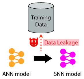
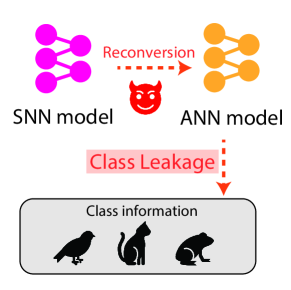
(a) During Conversion	(b) After Deployment

Figure 1: Illustration of data leakage and class leakage problems. (a) The data leakage problem is likely to happen when an ANN model accesses real data during conversion process. (b) The malicious attacker can obtain class information by reconverting the SNN model to the ANN model.

Among various SNN training algorithms, ANN-SNN conversion is well-established and achieves high performance on complex datasets. Here, pre-trained ANNs are converted to SNNs using weight or threshold balancing in order to replace Rectified Linear Unit (ReLU) activation with a spiking Leak-Integrate-and-Fire (LIF) activation (Sengupta et al. 2019; Han et al. 2020; Diehl et al. 2015; Rueckauer et al. 2017; Deng et al. 2022; Li et al. 2021b; Kim and Panda 2021a). Existing conversion algorithms are based on the assumption that the model can access the entire training data. Specifically, training samples are passed through a network and maximum activation value is used to calculate the layer-wise threshold or weight scaling constant. However, this may not always be feasible. Enterprises would not allow proprietary information to be shared publicly with other companies and individuals. Importantly, the training set may contain sensitive information, such as biometrics. Overall, such concerns motivates a line of research on privacy-preserving algorithms (Kundu et al. 2020; Nayak et al. 2019; Haroush et al. 2020; Liang, Hu, and Feng 2020). We refer to this problem as data leakage (Fig. 1(a)).

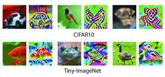
Figure 2: Examples of class leakage. We use VGG16 trained on CIFAR10 and Tiny-ImageNet. We visualize pair of images (left: real image, right: generated image) for each sample (CIFAR10: automobile, bird, and dog; Tiny-ImageNet: goldfish, bullfrog, and goose). The right image is generated using Algorithm 1.

In addition, we tackle the class leakage problem after deployment (i.e., inference), as shown in Fig. 1(b). It is a well-known fact that one can obtain a representative class image from model parameters by using simple gradient backpropagation (see Fig. 2) (Mopuri, Uppala, and Babu 2018; Yosinski et al. 2015). From a security perspective, revealing class information can induce critical threats in a neural system. A malicious attacker can find a blind spot in neural systems, and use these unrecognizable classes/pattern to disguise a system in real-world. Also, class information can be exploited to generate a strong adversarial attack (Goodfellow, Shlens, and Szegedy 2014). For instance, Mopuri et al.(Mopuri, Uppala, and Babu 2018) use synthetic class representation to generate universal adversarial perturbations. Therefore, to build a secure neural system, the class leakage problem should be addressed.

In this paper, we propose PrivateSNN, a new ANN-SNN conversion paradigm that addresses both data leakage and class leakage problems. Firstly, to address the data leakage issue, we generate synthetic data samples from the pre-trained ANN model and conduct ANN-SNN conversion using generated data. For the class leakage issue, we encrypt the weight parameters with a temporal spike-based learning rule. This stage optimizes the SNN parameters with the non-differentiable spiking LIF activation function, which prevents exact backward gradients calculation. Note, it is difficult to address the class leakage problem in ANN domain since precise backward gradients can be calculated. At the same time, considering the resource-constrained devices where SNNs are likely to be applied, SNNs might be limited to using a small number of training samples due to the computational cost for training. To preserve the performance with a small dataset, we distill the knowledge from ANN to regularize the SNN during spike-based training.

In summary, our key contributions are as follows: (i) So far, in SNN literature, there is no discussion about the privacy issue of ANN-SNN conversion. For the first time, we showcase the privacy issues and also propose ways to tackle them. (ii) We tackle two leakage problems (i.e., data leakage and class leakage) that are most likely to happen during conversion. (iii) We propose PrivateSNN which successfully converts ANNs to SNNs without exposing sensitive information of data. We encrypt the weight parameters of the converted SNN with a temporal learning rule. Also, distillation from ANN to SNN enables stable encryption training with a small number of training samples. (iv) We conduct extensive experiments on various datasets including CIFAR10, CIFAR100, and TinyImageNet and demonstrate the advantages of PrivateSNN for privacy and energy-efficiency.

Related Work

Spiking Neural Networks

Various SNN training techniques have been proposed in order to build efficient neuromorphic systems. Surrogate gradient learning techniques circumvent the non-differentiable problem of a Leak-Integrate-and-Fire (LIF) neuron by defining an approximate backward gradient function (Lee, Delbruck, and Pfeiffer 2016; Lee et al. 2020; Neftci et al. 2019). ANN-SNN conversion techniques convert pre-trained ANNs to SNNs using weight or threshold balancing to replace ReLU with LIF activation (Sengupta et al. 2019; Han et al. 2020; Diehl et al. 2015; Rueckauer et al. 2017; Li et al. 2021a). Compared to other methods, conversion yields SNNs with competitive accuracy as their ANN counterparts on a variety of tasks.

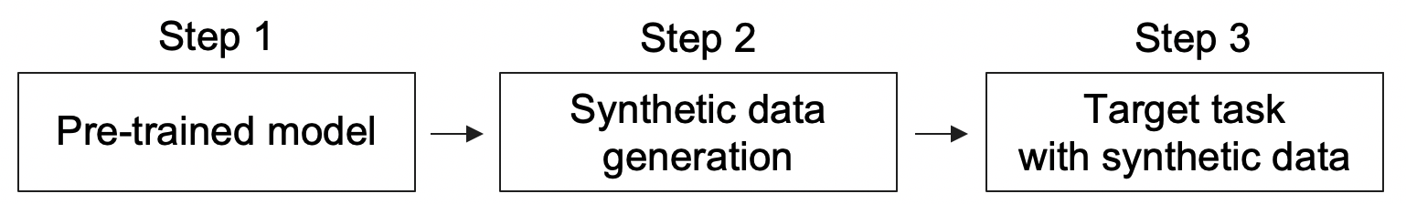
Figure 3: General approach for addressing data leakage.

Method	Data	Class
(✓: addressed / ✕: not addressed)	Leakage	Leakage
Private ANN approaches	✓	✕
(Haroush et al. 2020; Nayak et al. 2019)
ANN-SNN conversion	✕	✕
(Sengupta et al. 2019; Han et al. 2020)
SNN-surrogate gradients	✕	✓
(Lee et al. 2020; Zheng et al. 2020)
PrivateSNN (ours)	✓	✓

Table 1: Related work comparison.

Privacy-preserving Methods

Our approach for addressing data leakage is similar to previous privacy-preserving approaches in ANN domain (Haroush et al. 2020; Nayak et al. 2019). Most prior ANN works generate synthetic data from a pre-trained model and then train a model for a target task, as shown in Fig. 3. We conduct ANN-SNN conversion and show successful conversion performance with synthetic data. Note, no prior work before us has shown that SNNs can be converted without using the real dataset. Further, to the best of our knowledge, previous ANN or SNN approaches have not addressed the class leakage issue. To clarify the objective of our work, in Table 1, we compare the position of our work with privacy approaches in ANN domain as well as other SNN optimization methods. The previous privacy preserving ANN approaches successfully address data leakage but cannot resolve class leakage, since ANNs can calculate the exact gradients for reconstructing conceptual class images. The standard SNN optimization methods (i.e., ANN-SNN conversion and surrogate gradients learning) cannot address data leakage problem. Moreover, ANN-SNN conversion cannot address class leakage since SNNs have the same weights as ANNs, therefore the attacker can recover the original ANN model and perform concept reconstruction. On the other hand, surrogate gradients learning can prevent the class leakage problem since the weight parameters are trained with non-differentiable LIF activation function. Different from the previous methods, our PrivateSNN addresses both problems in a framework, by using data-free conversion and temporal spike-based training.

The Vulnerability of ANN-SNN Conversion

In this section, we present the ANN-SNN conversion algorithm and show the two possible leakage problems.

ANN-SNN Conversion

Our model is based on LIF neuron. We formulate the membrane potential $u_{i}^{t}$ of a single neuron $i$ as:

$$u_{i}^{t}=\lambda u_{i}^{t-1}+\sum_{j}w_{ij}o^{t}_{j},$$ (1)

where, $\lambda$ is a leak factor, $w_{ij}$ is a the weight of the connection between pre-synaptic neuron $j$ and post-synaptic neuron $i$. If the membrane potential $u_{i}^{t}$ exceeds a firing threshold $\theta$, the neuron $i$ generates spikes $o_{i}^{t}$. After the neuron fires, we perform a soft reset, where the membrane potential value $u_{i}^{t}$ is lowered by the threshold $\theta$.

We use the method described by (Sengupta et al. 2019) for implementing the ANN-SNN conversion. They normalize the weights or the firing threshold $\theta$ to take into account the actual SNN operation in the conversion process. The overall algorithm for the conversion method is detailed in Supplementary D. First, we copy the weight parameters of a pre-trained ANN to an SNN. Then, for every layer, we compute the maximum activation across all time-steps and set the firing threshold to the maximum activation value. The conversion process starts from the first layer and sequentially goes through deeper layers. Note that we do not use batch normalization (Ioffe and Szegedy 2015) since all input spikes have zero mean values. Also, following the previous works (Han et al. 2020; Sengupta et al. 2019; Diehl et al. 2015), we use Dropout (Srivastava et al. 2014) for both ANNs and SNNs.

Two Types of Leakage Problems

Data Leakage from Public Datasets: The entire training data is required to convert ANNs to SNNs (see Supplementary D). However, due to privacy issues, we might not be able to access the training samples. Even techniques such as, quantization, model compression, distillation, and domain adaptation have been shown to use synthetically generated data to deploy the final model to preserve privacy (Kundu et al. 2020; Kim, Cho, and Hong 2020; Nayak et al. 2019; Li et al. 2021a; Haroush et al. 2020; Liang, Hu, and Feng 2020). Therefore, there is a need to develop a data-free conversion algorithm in the neuromorphic domain.

Algorithm 1 Class representative image generation

Input: target class ($c$); max iteration ($N$); blurring frequency ($f_{blur}$); learning rate ($\eta$)
Output: class representative image $x$

1:$x$ $\leftarrow$ $U(0,1)$ $\triangleright$ Initialize input as uniform random distribution

2:for $n\leftarrow 1$ to $N$ do

3:     if $n$ % $f_{blur}==0$ then

4:         $x\leftarrow GaussianBlur(x)$

5:     end if

6:     $y$ $\leftarrow$ $network(x)$ $\triangleright$ compute pre-softmax output $y$

7:     $x$ $\leftarrow$ $x+\eta\frac{\partial y_{c}}{\partial x}$

8:end for

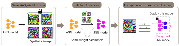
Figure 4: Overview of the proposed PrivateSNN. We first generate synthetic images based on underlying data distribution from a pre-trained ANN. Then, based on the generated samples, we convert the ANN to a SNN model. Finally, we encode synthetic images to spike signal, and train the converted SNN. The weight parameter is encrypted with temporal information. We deploy the final encrypted SNN model for inference.

Class Leakage from Reconverting SNNs to ANNs: In addition to data leakage, class information, e.g., pattern and shape of the object, also can be targeted by the attacker. Algorithm 1 presents a simple way to obtain class representative information from an ANN model. First, we initialize the input tensor with uniform random distribution. After that, we use an iterative optimization strategy where input noise is updated to maximize the pre-softmax logit $y_{c}$ of target class $c$. For every blur period $f_{blur}$, we smooth the image with Gaussian blur kernel since gradient at input layer has a high frequency (Yosinski et al. 2015). Fig. 2 shows examples of class representative images generated from a pre-trained model.

However, this technique is based on the assumption that we can compute the exact gradient for all layers. It is difficult to compute gradient value of SNNs due to the non-differentiable nature of LIF neuron (Eq. 1). Therefore, in order to generate proper class representation, the attacker should reconvert SNNs to ANNs. The re-conversion process depends on the type of conversion technique; weight scaling or threshold scaling. There are several conversion algorithms (Rueckauer et al. 2017; Diehl et al. 2015) that scale weight parameters of each layer. In such cases, the attacker cannot directly recover original ANN weights. However, each layer is scaled by a constant value, therefore the original ANN weights might be recovered by searching several combinations of layer-wise scaling factors. Recent state-of-the-art conversion algorithms (Sengupta et al. 2019; Han et al. 2020; Han and Roy 2020) use threshold scaling, i.e., change the thresholds while maintaining the weight parameters to obtain high performance. In our experiments, we use threshold scaling for ANN-SNN conversion and then, explore the class leakage issues. In this case, the original ANN can be reconverted by simply changing LIF neuron to ReLU neuron. With the reconverted ANN, the attacker can simply reconstruct class representation by backpropagation as shown in Algorithm 1. Overall, a non-linear weight encryption technique is required to make SNNs robust to class leakage.

Methodology

This section presents a detailed methodology for PrivateSNN. We first propose a data-free conversion method from a pre-trained ANN. Then, we describe how a temporal spike-based learning rule can encrypt weight parameters in SNNs. Fig. 4 illustrates the overall approach.

Data-Free Conversion for Data Leakage

Data Generation from a Pre-trained ANN: Without accessing real data, we generate synthetic images from a pre-trained ANN. Conversion performance relies on the maximum activation value of features, therefore synthetic images have to carefully reflect underlying data distribution from the pre-trained ANN. Nayak et al. (2019) take into account the relationship between classes in order to generate data, resulting in better performance on a distillation task. Following this pioneering work, we generate synthetic images based on class relationships from the weights of the last fully-connected layer. Specifically, we can define a weight vector $w_{c}$ between the penultimate layer and the class logit $c$ in the last layer. Then, we calculate the class similarity score between class $i$ and $j$:

$$s_{ij}=\frac{w_{i}^{T}w_{j}}{\|w_{i}\|_{2}^{2}\|w_{j}\|_{2}^{2}}.$$ (2)

Then, we sample a soft label based on Dirichlet distribution where a concentration parameter $\alpha_{c}$ is a class similarity vector of class $c$. For each class $c$, the class similarity vector consists of class similarity between class $c$ and other classes. For example, for class $1$ of CIFAR10 dataset, the concentration parameter is $\alpha_{1}=[s_{10},s_{11},s_{12},...,s_{19}]$. For a sampled soft label from Dirichlet distribution, we optimize input $x$ initialized with uniform random distribution. We collect the same number of samples for each class and exploit this synthetic dataset for conversion. The overall procedure for data-free conversion is shown in Algorithm 2 [Step1].

Algorithm 2 PrivateSNN Approach

Input: total class set ($C$); the number of samples per class ($N$); pre-trained ANN model ($ANN$); SNN model ($SNN$); spike time-step ($T$); distillation temperature ($\tau$);
Output: encrypted SNN model

1:[Step1] Data-free conversion

2:$D$ $\leftarrow$ $\O$$\triangleright$ Initialize synthetic dataset $D$

3:for $c\leftarrow 1$ to $C$ do

4:     $\alpha_{c}$ $\leftarrow$ $ANN.fc.weight$$\triangleright$ Compute class similarity

5:     for $n\leftarrow 1$ to $N$ do

6:         $y\sim Dir(\alpha_{c})$ $\triangleright$ Sample soft label from Dirichlet

7:         $x$ $\leftarrow$ $U(0,1)$ $\triangleright$ Initialize input

8:         Find $x$ that minimizes $L_{CE}(ANN(x),y)$

9:         $D\leftarrow D\cup\{x\}$

10:     end for

11:end for

12:Do ANN-SNN conversion with synthetic data $D$

13:[Step2] Encryption with spike-based learning

14:for $i\leftarrow 1$ to $max\_iter$ do

15:     fetch a mini batch $X\subset D$

16:     for $t\leftarrow 1$ to $T$ do

17:         O $\leftarrow$ PoissonGenerator(X)

18:         for $l\leftarrow 1$ to $L-1$ do

19:              $(O^{t}_{l},U_{l}^{t})\leftarrow(\lambda,U_{l}^{t-1},(W_{l},O^{t}_{l-1}))$ $\triangleright$ Eq. 1

20:         end for

21:         $U_{L}^{t}\leftarrow(U_{L}^{t-1},(W_{l},O^{t}_{L-1}))$ $\triangleright$ Final layer

22:     end for

23:     $L_{CE}\leftarrow(U_{L}^{T},Y)$

24:     $L_{KD}\leftarrow(ANN(X,\tau),SNN(X,\tau))$ $\triangleright$ Eq. 3

25:     Do back-propagation and weight update

26:end for

ANN-SNN Conversion with synthetic images: By generating synthetic images, we do not have to access the original dataset. Instead, we find the threshold of each layer from the maximum activation of synthetic images (see ANN-SNN Conversion algorithm in Supplementary D). Interestingly, we observe that converted SNNs with synthetic images almost recover the performance of the original ANN. This means that conversion process is feasible with inherent data distribution from a trained model. However, SNNs are still vulnerable to class leakage. If the attacker gets access to the weights of the SNN, they can easily recover the original ANN by simply changing the LIF neuron to ReLU. Therefore, we encrypt the converted SNN using the temporal spike-based learning rule (will be described in the next subsection). Note, we use a relatively small number of time-steps (e.g., 100 $\sim$ 150) for conversion. This is because short time-steps reduces training time and memory for post-conversion training. Also, short latency can bring more energy efficiency at inference. We observe that encryption training recovers the performance loss caused by using small number of time-steps for conversion.

Class Encryption with Spike-based Training

The key idea here is that training SNNs with temporal data representation makes class information difficult to be interpreted in the spatial domain.

Encoding static images with rate coding: In order to map static images to temporal signals, we use rate coding (or Poisson coding). Given the time window, rate coding generates spikes where the number of spikes is proportional to the pixel intensity. For time-step $t$, we generate a random number for each pixel $(i,j)$ with normal distribution ranging between $[I_{min},I_{max}]$, where $I_{min},I_{max}$ correspond to the minimum and maximum possible pixel intensity. After that, for each pixel location, we compare the pixel intensity with the generated random number. If the random number is greater than the pixel intensity, the Poisson spike generator outputs a spike with amplitude $1$. Otherwise, the Poisson spike generator does not yield any spikes. Overall, rate coding enables static images to span the temporal axis without huge information loss.

Training SNNs with spike-based learning: Given input spikes, we train converted SNNs based on gradient optimization. Intermediate LIF neurons accumulate pre-synaptic spikes and generate output spikes (Eq. 1). Spike information is passed through all layers and stacked or accumulated at the output layer (i.e., prediction layer) This enables the accumulated temporal spikes to be represented as probability distribution after the softmax function. From the accumulated membrane potential, we can define the cross-entropy loss for SNNs.

On-device distillation: One important thing we have to consider is the computational cost for post-conversion training. This is crucial to a limited-resource environment such as a mobile device with battery constraints. Also, SNNs require multiple feed-forward steps per one image, and thus are more energy-consuming compared to ANN training. In order to reduce the cost for training, we can reduce the number of synthetic training samples. However, with a small number of training samples, the networks easily overfit, resulting in performance degradation. To address this issue, we distill knowledge from ANNs to SNNs. Yuan et al. (2019) recently discovered the connection between knowledge distillation and label smoothing, which supports distillation improves the generalization power of the model. Thus, it is intuitive that if we use knowledge distillation during the spike-based training of the converted SNN, then the model is likely to show better generalization to small number of data samples. Therefore, the total loss function becomes the combination of cross-entropy loss and distillation loss:

$${L}=(1-m)L_{CE}+mL_{KD}(A(X,\tau),S(X,\tau)).$$ (3)

Here, $A(\cdot)$ and $S(\cdot)$ represent ANN and SNN models, respectively. Also, $\tau$ denotes distillation temperature, and $m$ is the balancing coefficient between two losses. Note that $L_{KD}$ is knowledge distillation loss (Hinton, Vinyals, and Dean 2015). The training samples $X$ used in this stage are a subset of the synthetically generated data used during conversion.

Based on Eq. 3, we compute the gradients of each layer $l$. Here, we use spatio-temporal back-propagation (STBP), which accumulates the gradients over all time-steps (Wu et al. 2018; Neftci et al. 2019). We can formulate the gradients at the layer $l$ by chain rule as:

$$\frac{\partial L}{\partial W_{l}}=\begin{cases}\sum_{t}(\frac{\partial L}{\partial O_{l}^{t}}\frac{\partial O_{l}^{t}}{\partial U_{l}^{t}}+\frac{\partial L}{\partial U_{l}^{t+1}}\frac{\partial U_{l}^{t+1}}{\partial U_{l}^{t}})\frac{\partial U_{l}^{t}}{\partial W_{l}},&\text{if $l:$ hidden }\\ \frac{\partial L}{\partial U_{l}^{T}}\frac{\partial U_{l}^{T}}{\partial W_{l}}.&\text{if $l:$ output}\end{cases}$$ (4)

Here, $O^{t}_{l}$ and $U^{t}_{l}$ are output spikes and membrane potential at time-step $t$ for layer $l$, respectively. For the output layer, we get the derivative of the loss $L$ with respect to the membrane potential $u_{i}^{T}$ at final time-step $T$, which is continuous and differentiable for all possible membrane potential values. On the other hand, LIF neurons in hidden layers generate spike output only if the membrane potential $u_{i}^{t}$ exceeds the firing threshold, leading to non-differentiability. To deal with this problem, we introduce an approximate gradient:

$$\frac{\partial o_{i}^{t}}{\partial u_{i}^{t}}=\max\{0,1-\ |\frac{u_{i}^{t}-\theta}{\theta}\ |\}.$$ (5)

Overall, we update the network parameters at the layer $l$ based on the gradient value (Eq. 4) as $W_{l}=W_{l}-\eta\Delta W_{l}$. The procedure for spike-based training for encrypting the model is detailed in Algorithm 2 [Step2].

Attack Scenarios for Class Leakage

In this section, we present two possible attack scenarios on class leakage. Since we do not access the original training data, the data leakage problem is addressed. Therefore, here we only discuss the class leakage problem.

Attack scenario 1 (Reconverting SNN to ANN): As discussed earlier, the attacker might copy the weights of SNN and recover the original ANN. By using the re-converted ANN, the attacker optimizes the input noise based on Algorithm 1. Without post-conversion encryption training, the attacker simply reconstructs class representation by backpropagation. However, if we use spike-based training, the weight of SNN is fully encrypted in the spatial domain.

Attack scenario 2 (Directly generate class representation from SNN): The attacker might directly backpropagate gradients in SNN architecture and reconstruct class representation. Thus, this is the SNN version of Algorithm 1. The technical problem here is that LIF neurons and Poisson spike generation process are non-differentiable. To address this issue, we use approximated gradient functions (Eq. 5) for LIF neurons. Also, in order to convert the gradient in the temporal domain to the spatial domain, we accumulate gradient at the first convolution layer. After that, we deconvolve the accumulated gradients with weights of the first layer. These deconvolved gradients have a similar value with original gradients of images before the Poisson spike generator, which has been validated in previous work (Sharmin et al. 2020). Thus, we can get a gradient $\delta x$ converted into spatial domain, and the input noise is updated with gradient $\delta x$ scaled by $\zeta$. Algorithm 3 illustrates the overall optimization process. However, this attack does not show meaningful features due to the discrepancy between real gradients and approximated gradients. This supports that SNN model itself is robust to gradient-based security attacks (Roy, Jaiswal, and Panda 2019; Sharmin et al. 2020). We show the qualitative results for Attack 1, 2 scenarios in Fig. 6.

Algorithm 3 Directly generate class representation from SNNs (Attack scenario 2)

Input: target class ($c$); max iteration ($N$); scaling factor ($\zeta$); SNN model (SNN); spike time-step ($T$)
Output: class representative image $x$

1:$x$ $\leftarrow$ $U(0,1)$ $\triangleright$ Initialize input

2:$W_{1}$ $\leftarrow$ $SNN.conv1.weight$$\triangleright$ First convolution weight

3:$G=0$$\triangleright$ Accumulated gradient at the first conv layer

4:for $n\leftarrow 1$ to $N$ do

5:     for $t\leftarrow 1$ to $T$ do

6:         $y\leftarrow SNN(x_{t})$

7:         $G+=\frac{1}{T}\frac{\partial y_{c}}{\partial x_{conv1}}$ $\triangleright$ Accumulate gradients in layer 1

8:     end for

9:     $\delta x\leftarrow Deconvolution(W_{1},G)$ $\triangleright$ Deconvolution

10:     $x$ $\leftarrow$ $x+\zeta\delta x$

11:end for

Experiments

Experimental Setting

We evaluate our PrivateSNN on three public datasets (i.e., CIFAR-10 (Krizhevsky and Hinton 2009), CIFAR-100 (Krizhevsky and Hinton 2009), Tiny-ImageNet (deng2009imagenet)). Our implementation is based on Pytorch (Paszke et al. 2017). For conversion, we apply threshold scaling technique as proposed in (Han et al. 2020). For post-conversion training, we use Adam with base learning rate 1e-4. Here, we use 5000, 10000, 10000 synthetic samples for training SNNs on CIFAR10, CIFAR100, and TinyImageNet, respectively. We use step-wise learning rate scheduling with a decay factor of 10 at 50% and 70% of the total number of epochs. We set the total number of epochs to 20 for all datasets. For on-device distillation, we set $m$ and $\tau$ to $0.7$ and $20$ in Eq. 3, respectively. For class representation, we set $f_{blur}$ and $\eta$ in Algorithm 1 to 4 and 6, respectively. For attack scenario 2 in Algorithm 3, we set $\zeta$ to 0.01. All detailed experimental setup and hyperparameters are described in Supplementary B. Note that our objective is to showcase the advantages of PrivateSNN for tackling data and class leakage.

Performance Comparison

Before we present the experimental results, we define the terms used in our method: Data-free Conversion (DC), Class Encryption Training (CET), and On-device Distillation (OD). We call our final method as PrivateSNN, thus, PrivateSNN = DC + CET + OD.

Surprisingly, we find that PrivateSNN encrypts the networks without significant performance loss. Table 2 shows the performance of reference ANN (i.e., VGG16) and previous conversion methods which uses training data. Here, we use Sengupta et al. (2019); Han et al. (2020); Zambrano et al. (2019) as representative state-of-the-art conversion methods for comparison. The results show that our PrivateSNN can be designed without a huge performance drop across all datasets. This implies that synthetic samples generated from the ANN model contain enough information for a successful conversion and post-training processes.

In Table 3, we conduct ablation studies on each component (i.e., DC, CET, and OD) of our method. Here, we present the robustness of model on data leakage and class leakage and compare the number of training samples, and classification accuracy. With DC, the SNN model can address data leakage, however, it is still vulnerable to class leakage. Adding CET on DC resolves class leakage with performance improvement. However, an insufficient number of training samples cannot achieve near state-of-the-art performance. Finally, using OD helps the networks to improve the performance with a limited number of samples.

Method	Require	Dataset	Acc (%)
	train data?
VGG16	-	CIFAR10	91.6
Rueckauer et al. (2017)	Yes	CIFAR10	90.9
Sengupta et al. (2019)	Yes	CIFAR10	91.5
Han et al. (2020)	Yes	CIFAR10	91.4
Zambrano et al. (2019)	Yes	CIFAR10	89.7
PrivateSNN (ours)	No	CIFAR10	89.2
VGG16	-	CIFAR100	64.3
Sengupta et al. (2019)	Yes	CIFAR100	62.7
Zambrano et al. (2019)	Yes	CIFAR100	63.4
PrivateSNN (ours)	No	CIFAR100	62.3
VGG16	-	TinyImgNet	51.9
Sengupta et al. (2019)	Yes	TinyImgNet	50.6
PrivateSNN (ours)	No	TinyImgNet	50.7

Table 2: Classification Accuracy (%) on CIFAR10, CIFAR100, and TinyImageNet. We report the accuracy of VGG16 (pre-trained ANN) (Simonyan and Zisserman 2014) architecture in our experiments as a reference.

Method	D.L.	C.L.	# Train data	Acc (%)
DC (T=150)	✓	✕	-	82.8
DC + CET	✓	✓	5000	86.9
DC + CET + OD	✓	✓	5000	89.2

Table 3: Ablation study for each component in our method on CIFAR10 dataset (✓: addressed / ✕: not addressed). D.L / C.L. denote data leakage and class leakage, respectively.

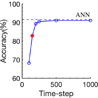
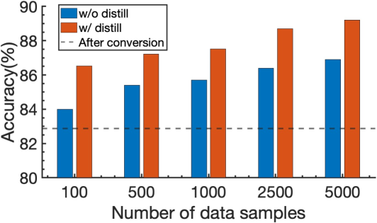
(a)	(b)

Figure 5: (a) Data-free Conversion performance. We use a small number of time-steps for efficient post-conversion training (marked by red dot). (b) Performance with respect to the number of training samples using encryption training. For both experiments, we use VGG16 trained on CIFAR10.

Analysis on Data-free Conversion

In Fig. 5(a), we measure the data-free conversion performance with respect to the number of time-steps in the conversion process. The results show that the data-free SNN conversion model can almost recover the original ANN performance with large number of time-steps (i.e., $\geq 500$). But, we use a small number of time-steps (i.e., $\leq 200$) to perform the conversion and then, perform CET in the low time-step regime. Here, we only show CIFAR10 results. The CIFAR100, and TinyImageNet results are shown in Supplementary E. Specifically, PrivateSNN is trained with time-step 150, 200, and 200 for CIFAR10, CIFAR100, and TinyImageNet, This is because smaller time-steps bring more energy-efficiency during both training and inference. Also, we observe that encryption training with distillation recovers the accuracy even though SNNs are converted in a low time-step regime (Table 3).

Effect of Distillation in Encryption Training

After converting ANNs to SNNs, we train the networks with synthetic images. In order to figure out how many samples are required for post training, we show the performance with respect to the number of synthetic samples in Fig. 5(b). Note, data-free conversion at 150 time-steps achieves 82.8 % accuracy (black dotted line in the figure). The results show that encryption training (without distillation) degrades the performance with a small number of samples. Interestingly, with distillation, the network almost preserves the performance regardless of sample size. Thus, distillation is an effective regularization method for spike-based learning with a small number of synthetic images.

Method	w/o Encryption	w/ Encryption
Attack scenario 1	354.8	448.2
Attack scenario 2	447.9	422.4

Table 4: FIDs between test set and generated images from reconverted ANN (Attack scenario 1) and backward gradients on SNNs (Attack scenario 2) on CIFAR10. Higher FID implies lower leakage.

Robustness on Class Leakage Problem

To validate the robustness of PrivateSNN against Attack scenario 1 and Attack scenario 2 (two most likely class leakage scenarios), we synthesize the class representation of SNNs with (w/) and without (w/o) class encryption training (CET). Fig. 6 shows 8 examples of generated images from CIFAR10 (The results from CIFAR100, and TinyImageNet are shown in Supplementary H). We visualize images from five configurations: original images, Attack1 w/o CET, Attack1 w/ CET, Attack2 w/o CET, and Attack2 w/ CET. We observe that SNNs without CET (i.e., simply, data free converted SNNs) are vulnerable to Attack1, showing important features of original classes (see Fig. 6(b)). On the other hand, with temporal spike-based learning rule, Attack1 does not discover any meaningful information as shown in Fig. 6(c). For Attack2 (Fig. 6(d) and Fig. 6(e)), synthetic images show noisy results due to discrepancy between real gradients and approximated gradients. This comes from the intrinsic nature of SNNs, therefore SNNs are robust to Attack2 even without encryption. Overall, PrivateSNN is an effective solution to class leakage problem.

We quantify the security of the model by measuring how much generated images represent similar features with that of original images. To this end, we use Fr̀echet inception distance (FID) metric (Heusel et al. 2017) that is widely used in GAN evaluation (Miyato and Koyama 2018; Miyato et al. 2018). The FID score compares the statistics of embedded features in a feature space (see Supplementary C for more detailed explanation). Thus, a lower FID score means that the generated images provide the original data-like feature. In Table 4, the SNN model without encryption training on attack scenario 1 achieves a much lower FID score (i.e., 354.8) compared to others, which supports our visualization results.

Energy-efficiency of PrivateSNN

For the sake of complete analysis, we calculate the inference energy of PrivateSNN and compare with ANN and other conversion methods. Note that, we use the same energy estimation model as (Panda, Aketi, and Roy 2020), which is rather a rough estimate that considers only Multiply and Accumulate (MAC) operations and neglects memory and peripheral circuit energy. We calculate the energy based on spike rate (i.e., the average number of spikes across time) of all layers (see Supplementary F for details). In Table 5, we compare the energy efficiency between VGG16, standard conversion (Sengupta et al. 2019; Han et al. 2020), and our method. The results show that PrivateSNN is more efficient than both ANN as well as a standard converted SNN. This implies our approach of $DC+CET+OD$ lowers the overall spike rate which makes PrivateSNN more energy-efficient.

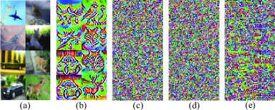
Figure 6: Qualitative results (CIFAR10) of two attack scenarios on the class leakage problem. (a) Original Data. (b) Attack1-w/o CET. (c) Attack1-w/ CET. (d) Attack2-w/o CET. (e) Attack2-w/ CET.

Method	Timestep	Acc (%)	$\frac{E_{ANN}}{E_{ours}}$
VGG16 (ANN)	1	91.5	1$\times$
Sengupta et al. (2019)	500	91.2	27.9$\times$
Han et al. (2020)	250	91.4	53.9$\times$
PrivateSNN (ours)	150	89.2	55.8$\times$

Table 5: Energy efficiency comparison on VGG16-CIFAR10.

Conclusion

For the first time, we expose the vulnerability of converted SNNs to data and class leakage. We propose PrivateSNN that comprises of data-free conversion followed by weight encryption with spike-based training on synthetic data to tackle the privacy issues. We further optimize the training process with distillation that enables stable encryption training with very few training samples. So far, the discussion around SNNs has more or less been limited to energy-efficiency. This work sets precedence on the vulnerabilities unique to the SNN domain and also showcases the benefits of temporal spike-based learning for encryption. We hope this fosters future work around security and privacy in SNNs. One limitation of data-free conversion is that the conversion performance is reduced with the overfitted networks which are likely to generate biased data representation. We discuss such limitation in Supplementary.

References

- Akopyan et al. (2015) Akopyan, F.; Sawada, J.; Cassidy, A.; Alvarez-Icaza, R.; Arthur, J.; Merolla, P.; Imam, N.; Nakamura, Y.; Datta, P.; Nam, G.-J.; et al. 2015. Truenorth: Design and tool flow of a 65 mw 1 million neuron programmable neurosynaptic chip. IEEE transactions on computer-aided design of integrated circuits and systems, 34(10): 1537–1557.
- Christensen et al. (2022) Christensen, D. V.; Dittmann, R.; Linares-Barranco, B.; Sebastian, A.; Le Gallo, M.; Redaelli, A.; Slesazeck, S.; Mikolajick, T.; Spiga, S.; Menzel, S.; et al. 2022. 2022 roadmap on neuromorphic computing and engineering. Neuromorphic Computing and Engineering.
- Davies et al. (2018) Davies, M.; Srinivasa, N.; Lin, T.-H.; Chinya, G.; Cao, Y.; Choday, S. H.; Dimou, G.; Joshi, P.; Imam, N.; Jain, S.; et al. 2018. Loihi: A neuromorphic manycore processor with on-chip learning. IEEE Micro, 38(1): 82–99.
- Deng et al. (2022) Deng, S.; Li, Y.; Zhang, S.; and Gu, S. 2022. Temporal Efficient Training of Spiking Neural Network via Gradient Re-weighting. arXiv preprint arXiv:2202.11946.
- Diehl and Cook (2015) Diehl, P. U.; and Cook, M. 2015. Unsupervised learning of digit recognition using spike-timing-dependent plasticity. Frontiers in computational neuroscience, 9: 99.
- Diehl et al. (2015) Diehl, P. U.; Neil, D.; Binas, J.; Cook, M.; Liu, S.-C.; and Pfeiffer, M. 2015. Fast-classifying, high-accuracy spiking deep networks through weight and threshold balancing. In 2015 International Joint Conference on Neural Networks (IJCNN), 1–8. ieee.
- Fang et al. (2019) Fang, Y.; Wang, Z.; Gomez, J.; Datta, S.; Khan, A. I.; and Raychowdhury, A. 2019. A swarm optimization solver based on ferroelectric spiking neural networks. Frontiers in neuroscience, 13: 855.
- Frady et al. (2020) Frady, E. P.; Orchard, G.; Florey, D.; Imam, N.; Liu, R.; Mishra, J.; Tse, J.; Wild, A.; Sommer, F. T.; and Davies, M. 2020. Neuromorphic Nearest Neighbor Search Using Intel’s Pohoiki Springs. In Proceedings of the Neuro-inspired Computational Elements Workshop, 1–10.
- Furber et al. (2014) Furber, S. B.; Galluppi, F.; Temple, S.; and Plana, L. A. 2014. The spinnaker project. Proceedings of the IEEE, 102(5): 652–665.
- Goodfellow, Shlens, and Szegedy (2014) Goodfellow, I. J.; Shlens, J.; and Szegedy, C. 2014. Explaining and harnessing adversarial examples. arXiv preprint arXiv:1412.6572.
- Han and Roy (2020) Han, B.; and Roy, K. 2020. Deep Spiking Neural Network: Energy Efficiency Through Time based Coding. In Proc. IEEE Eur. Conf. Comput. Vis.(ECCV), 388–404.
- Han et al. (2020) Han, B.; et al. 2020. RMP-SNN: Residual Membrane Potential Neuron for Enabling Deeper High-Accuracy and Low-Latency Spiking Neural Network. In Proceedings of the IEEE/CVF Conference on Computer Vision and Pattern Recognition, 13558–13567.
- Haroush et al. (2020) Haroush, M.; Hubara, I.; Hoffer, E.; and Soudry, D. 2020. The knowledge within: Methods for data-free model compression. In Proceedings of the IEEE/CVF Conference on Computer Vision and Pattern Recognition, 8494–8502.
- He et al. (2016) He, K.; Zhang, X.; Ren, S.; and Sun, J. 2016. Deep residual learning for image recognition. In Proceedings of the IEEE conference on computer vision and pattern recognition, 770–778.
- Heusel et al. (2017) Heusel, M.; Ramsauer, H.; Unterthiner, T.; Nessler, B.; and Hochreiter, S. 2017. Gans trained by a two time-scale update rule converge to a local nash equilibrium. arXiv preprint arXiv:1706.08500.
- Hinton, Vinyals, and Dean (2015) Hinton, G.; Vinyals, O.; and Dean, J. 2015. Distilling the knowledge in a neural network. arXiv preprint arXiv:1503.02531.
- Ioffe and Szegedy (2015) Ioffe, S.; and Szegedy, C. 2015. Batch normalization: Accelerating deep network training by reducing internal covariate shift. arXiv preprint arXiv:1502.03167.
- Kim et al. (2019) Kim, S.; Park, S.; Na, B.; and Yoon, S. 2019. Spiking-yolo: Spiking neural network for real-time object detection. arXiv preprint arXiv:1903.06530, 1.
- Kim, Cho, and Hong (2020) Kim, Y.; Cho, D.; and Hong, S. 2020. Towards Privacy-Preserving Domain Adaptation. IEEE Signal Processing Letters, 27: 1675–1679.
- Kim and Panda (2020) Kim, Y.; and Panda, P. 2020. Revisiting batch normalization for training low-latency deep spiking neural networks from scratch. Frontiers in neuroscience, 1638.
- Kim and Panda (2021a) Kim, Y.; and Panda, P. 2021a. Optimizing deeper spiking neural networks for dynamic vision sensing. Neural Networks, 144: 686–698.
- Kim and Panda (2021b) Kim, Y.; and Panda, P. 2021b. Visual explanations from spiking neural networks using inter-spike intervals. Scientific reports, 11(1): 1–14.
- Krizhevsky and Hinton (2009) Krizhevsky, A.; and Hinton, G. 2009. Learning multiple layers of features from tiny images. Technical Report 0, University of Toronto, Toronto, Ontario.
- Kundu et al. (2020) Kundu, J. N.; Venkat, N.; Babu, R. V.; et al. 2020. Universal source-free domain adaptation. In Proceedings of the IEEE/CVF Conference on Computer Vision and Pattern Recognition, 4544–4553.
- Lee et al. (2020) Lee, C.; Sarwar, S. S.; Panda, P.; Srinivasan, G.; and Roy, K. 2020. Enabling spike-based backpropagation for training deep neural network architectures. Frontiers in Neuroscience, 14.
- Lee, Delbruck, and Pfeiffer (2016) Lee, J. H.; Delbruck, T.; and Pfeiffer, M. 2016. Training deep spiking neural networks using backpropagation. Frontiers in neuroscience, 10: 508.
- Li et al. (2021a) Li, Y.; Deng, S.; Dong, X.; Gong, R.; and Gu, S. 2021a. A free lunch from ANN: Towards efficient, accurate spiking neural networks calibration. In International Conference on Machine Learning, 6316–6325. PMLR.
- Li et al. (2021b) Li, Y.; Guo, Y.; Zhang, S.; Deng, S.; Hai, Y.; and Gu, S. 2021b. Differentiable Spike: Rethinking Gradient-Descent for Training Spiking Neural Networks. Advances in Neural Information Processing Systems, 34.
- Liang, Hu, and Feng (2020) Liang, J.; Hu, D.; and Feng, J. 2020. Do we really need to access the source data? source hypothesis transfer for unsupervised domain adaptation. In International Conference on Machine Learning, 6028–6039. PMLR.
- Miyato et al. (2018) Miyato, T.; Kataoka, T.; Koyama, M.; and Yoshida, Y. 2018. Spectral normalization for generative adversarial networks. arXiv preprint arXiv:1802.05957.
- Miyato and Koyama (2018) Miyato, T.; and Koyama, M. 2018. cGANs with projection discriminator. arXiv preprint arXiv:1802.05637.
- Mopuri, Uppala, and Babu (2018) Mopuri, K. R.; Uppala, P. K.; and Babu, R. V. 2018. Ask, acquire, and attack: Data-free uap generation using class impressions. In Proceedings of the European Conference on Computer Vision (ECCV), 19–34.
- Nayak et al. (2019) Nayak, G. K.; Mopuri, K. R.; Shaj, V.; Radhakrishnan, V. B.; and Chakraborty, A. 2019. Zero-shot knowledge distillation in deep networks. In International Conference on Machine Learning, 4743–4751. PMLR.
- Neftci et al. (2019) Neftci, E. O.; et al. 2019. Surrogate gradient learning in spiking neural networks. IEEE Signal Processing Magazine, 36: 61–63.
- Panda, Aketi, and Roy (2020) Panda, P.; Aketi, S. A.; and Roy, K. 2020. Toward scalable, efficient, and accurate deep spiking neural networks with backward residual connections, stochastic softmax, and hybridization. Frontiers in Neuroscience, 14.
- Paszke et al. (2017) Paszke, A.; Gross, S.; Chintala, S.; Chanan, G.; Yang, E.; DeVito, Z.; Lin, Z.; Desmaison, A.; Antiga, L.; and Lerer, A. 2017. Automatic differentiation in PyTorch. In NIPS-W.
- Roy, Jaiswal, and Panda (2019) Roy, K.; Jaiswal, A.; and Panda, P. 2019. Towards spike-based machine intelligence with neuromorphic computing. Nature, 575(7784): 607–617.
- Rueckauer et al. (2017) Rueckauer, B.; Lungu, I.-A.; Hu, Y.; Pfeiffer, M.; and Liu, S.-C. 2017. Conversion of continuous-valued deep networks to efficient event-driven networks for image classification. Frontiers in neuroscience, 11: 682.
- Sengupta et al. (2019) Sengupta, A.; Ye, Y.; Wang, R.; Liu, C.; and Roy, K. 2019. Going deeper in spiking neural networks: Vgg and residual architectures. Frontiers in neuroscience, 13: 95.
- Sharmin et al. (2020) Sharmin, S.; Rathi, N.; Panda, P.; and Roy, K. 2020. Inherent Adversarial Robustness of Deep Spiking Neural Networks: Effects of Discrete Input Encoding and Non-Linear Activations. arXiv preprint arXiv:2003.10399.
- Simonyan and Zisserman (2014) Simonyan, K.; and Zisserman, A. 2014. Very deep convolutional networks for large-scale image recognition. arXiv preprint arXiv:1409.1556.
- Srivastava et al. (2014) Srivastava, N.; Hinton, G.; Krizhevsky, A.; Sutskever, I.; and Salakhutdinov, R. 2014. Dropout: a simple way to prevent neural networks from overfitting. The journal of machine learning research, 15(1): 1929–1958.
- Venkatesha et al. (2021) Venkatesha, Y.; Kim, Y.; Tassiulas, L.; and Panda, P. 2021. Federated learning with spiking neural networks. IEEE Transactions on Signal Processing, 69: 6183–6194.
- Wu et al. (2018) Wu, Y.; Deng, L.; Li, G.; Zhu, J.; and Shi, L. 2018. Spatio-temporal backpropagation for training high-performance spiking neural networks. Frontiers in neuroscience, 12: 331.
- Yosinski et al. (2015) Yosinski, J.; Clune, J.; Nguyen, A.; Fuchs, T.; and Lipson, H. 2015. Understanding neural networks through deep visualization. arXiv preprint arXiv:1506.06579.
- Yuan et al. (2019) Yuan, L.; Tay, F. E.; Li, G.; Wang, T.; and Feng, J. 2019. Revisit knowledge distillation: a teacher-free framework. arXiv preprint arXiv:1909.11723.
- Zambrano et al. (2019) Zambrano, D.; Nusselder, R.; Scholte, H. S.; and Bohté, S. M. 2019. Sparse computation in adaptive spiking neural networks. Frontiers in neuroscience, 12: 987.
- Zheng et al. (2020) Zheng, H.; Wu, Y.; Deng, L.; Hu, Y.; and Li, G. 2020. Going deeper with directly-trained larger spiking neural networks. arXiv preprint arXiv:2011.05280.