A New Blind Asteroid Detection Scheme

Abstract

As astronomical photometric surveys continue to tile the sky repeatedly, the potential to push detection thresholds to fainter limits increases; however, traditional digital-tracking methods cannot achieve this efficiently beyond time scales where motion is approximately linear. In this paper we prototype an optimal detection scheme that samples under a user defined prior on a parameterization of the motion space, maps these sampled trajectories to the data space, and computes an optimal signal-matched filter for computing the signal to noise ratio of trial trajectories. We demonstrate the capability of this method on a small test data set from the Dark Energy Camera. We recover the majority of asteroids expected to appear and also discover hundreds of new asteroids with only a few hours of observations. We conclude by exploring the potential for extending this scheme to larger data sets that cover larger areas of the sky over longer time baselines.

1 Introduction

The vast majority of objects that exist within the solid angle of an astronomical exposure are undetectable above the noise of the image. Typical detection schemes employ a point spread function (PSF) or other convolution-based detection method and define “detections” as fluctuations above some threshold, typically measured in units of the signal-to-noise ratio (SNR). The number of false positives grows as this threshold is lowered such that a threshold below $\text{SNR}=5$ is rare and below $\text{SNR}=3$ is not typically useful for large, modern cameras. The most straightforward way to improve detection sensitivity is to increase the exposure time, but moving objects exhibit trailing losses and this does not allow for the removal of cosmic rays and other imprinted correlated noise that appear differently in each exposure and add over time. A common method for increasing detection sensitivity is taking multiple exposures and stacking the images and performing object detection on the median stack of the images. This reduces the noise proportional to the square root of the number of exposures (assuming equal exposure times and similar, uncorrelated noise in each), and thus allows for fainter detection thresholds. This method works well with modern cameras which have small read noise and dark current. Faint stars and galaxies are frequently observed for hours using this method.

Methods to stack the signal of moving objects are more challenging in practice. Large scale asteroid surveys such as the Catalina Sky Survey (CSS; Larson et al., 1998), the Panoramic Survey Telescope and Rapid Response System (Chambers et al., 2016, Pan-STARRS;[), and the Zwicky Transient Facility (ZTF; Masci et al., 2019) do not detect moving objects systematically with such methods. Instead, each of these surveys implement a similar method where objects are detected above an SNR threshold in single-epochs before they are linked together into orbital tracks and monitored until a confident orbital determination is made. The Pan-STARRS Moving Object Processing System (MOPS; Denneau et al., 2013) is an example method, which is also forming the basis for the method used by the upcoming Legacy Survey of Space and Time (LSST, formerly the Large Synoptic Survey Telescope; Ivezić et al., 2019), which will utilize a MOPS-like framework and report tracklets to the Minor Planet Center (MCP: Williams et al., 2009).

On the other hand, special surveys for moving objects have been carried out in order to go deeper than these single-epoch methods allow. It is informative to first consider the angular rate of motion of various classes of solar system objects of interest. The furthest comets, asteroids and Kuiper Belt objects (KBOs) move slowly enough to permit (without trailing losses) exposures of up to $\sim$20 minutes; whereas inner solar-system asteroids in the main-belt (MBAs) and near-Earth objects (NEOs) permit exposures of $\sim$2 minutes and as short as $\sim$1 second, respectively (Shao et al., 2014; Heinze et al., 2015). In order to overcome this motion, “digital tracking” methods have been developed. Digital tracking refers to the stacking of consecutive short exposures (short enough to avoid substantial trailing losses) along moving trajectories in order to add the signal of a moving object. This gives the benefits of tracking the motion of a moving object and taking a long exposure, with the added benefit of simpler removal of stationary objects through standard difference imaging. Furthermore, by not assuming the motion of the objects of interest, the intrinsic scatter in angular motion between moving objects may be probed generically by stacking along a fine grid in angular motion space and detecting objects on “shifted” median stacks (due to this methodology, this technique is also often known colloquially as “shift-and-stack”).

Tyson et al. (1992) first applied this method to search for KBOs, which resulted in a null detection but demonstrated the capability to search for moving objects down to faint limits without dealing with trailing losses. Later, Cochran et al. (1995) demonstrated the power of this method, by discovering a large population of KBOs with $m_{V}\leq 28$ using the Hubble Space Telescope (HST). Bernstein et al. (2004) also used HST to conduct a search for trans-Neptunian objects (TNOs) complete at the 50%-level down to $m_{606W}\leq 29.2$. More recently, Shao et al. (2014) and Zhai et al. (2014) used this method for fast moving NEOs, and Heinze et al. (2015) used it to search for MBAs. In the last year, authors have implemented faster searches with graphical processing units (GPUs) and massively parallel analyses capable of searching a finer grid and stacking a deeper stack of short exposures (Zhai et al., 2019; Whidden et al., 2019). Additionally, digital tracking has been used to estimate more precise astrometry, which is vital for fast moving objects for accurate orbit determination (Zhai et al., 2018). Most recently, Heinze et al. (2019) has used it to conduct a complete search for MBAs down to $m_{V}=25$.

In each of these studies, a linear assumption was made in order to avoid smearing the signal, which is an inherent cap on the usefulness of this technique. In this paper, we will describe a method that relaxes this requirement and enables a fully blind search for moving objects within survey data. A fully implemented version of our method could bring wide-area, long time-domain searches into play for digital tracking methods. We develop this method with an eye toward LSST (Ivezić et al., 2019), which will probe 2$\times 10^{5}$ square degrees to a $\text{SNR}=5$ depth of $m(r)=27.5$ by stacking $\sim 1000$ images per pointing in six filters (ugrizy). It will likely detect hundreds of thousands of asteroids over the ten-year survey with single-epoch detection methods. Our method is suitable for detecting asteroids in wide field surveys well below the single-epoch detection limit while also recovering valuable orbital and astrometric information simultaneously. In §2 we describe our test data from the Dark Energy Camera (DECam; Flaugher et al., 2015) mounted on the 4m Blanco Telescope at Cerro-Tololo Inter-American Observatory (CTIO) in Chile. In §3 we describe our detection method. We analyze our test data and present our results in §4. Finally, in §5 we offer a discussion of future extensions to this method and contextualize our simple test here in this larger picture.

2 Data

2.1 Observations

We obtained $\sim 3$ hours of observations on the Blanco Telescope at CTIO with DECam. These were spread over two consecutive nights (2018 December 22 and 23) during a 90 minute gap in the observability of the scheduled observations (Program 2018A-0273; PALS, PI William Dawson). The moon was full on 2018 December 21, so the nights were in bright time. In each night, we observed a single pointing toward the ecliptic plane, separated by a pro-grade translation of 1$\arcdeg$ day^-1 along the ecliptic. Each night consisted of a $\sim 90$ minutes stack of 40 second exposures in a single filter. We dithered randomly by selecting pointings from $\mathcal{N}(\mu_{RA},\sigma_{RA}^{2})$ and $\mathcal{N}(\mu_{DEC.},\sigma_{DEC}^{2})$, where $\mu_{RA}$ and $\mu_{DEC}$ are listed in Table 1 and $\sigma_{RA}=\sigma_{DEC}=2\arcmin$. The pointings over the two nights are shown also in Figure 1.

Table 1: Summary of observations

Date	Filter	Exposures	$\mu_{RA}$	$\mu_{DEC}$	Median Seeing
		Number	∘	∘	$\arcsec$
2018 Dec 22	r	85	135.00	17.04	0.97
2018 Dec 23	r	82	136.01	16.77	0.87

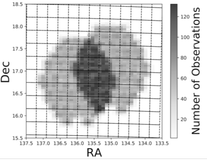
Figure 1: The data cube depth (number of frames) in R.A. and Dec. To generate the data cube, we cut the entire region into “patches” with the LSST data management pipeline, followed by creation of a master pixel grid. All analyses occurred on this grid.

2.2 Data Reduction

We obtained our exposures after standard processing by the DECam Community Pipeline (Valdes et al., 2014). We then used the LSST software package (Bosch et al., 2019) to produce difference images. This can be split into three different pieces: making calibrated single epoch catalogs and images, creating a static template image, and subtracting the template from the single epoch images to produce difference images.

The LSST stack single epoch processing includes: the masking of cosmic rays, measuring the PSF, detecting objects, deblending and measuring individual sources and calibrating the astrometry and photometry. A detailed explanation of each of these steps is explained in the HSC data release papers (Aihara et al., 2018, 2019). For calibration purposes we used the Pan-STARRS catalog (Flewelling et al., 2016).

To create the template images we first interpolated the data onto a tangent plane projection centered on the average pointing. The total observed area was divided into a regular grid with each grid $4000\times 4000$ pixels or $\sim 17\arcmin$ on a side (see Figure 1). For the templates we selected the best seeing images which were those with $\text{seeing}<1.2\arcsec$. For each grid the static sky is constructed following the procedure outlined in (Aihara et al., 2018, 2019). Briefly, the procedure builds a two-sigma clipped coadd to construct a static image of the sky. We subtract this coadd from each individual image and identify variable sources. Those detections that are truly variable will only appear in a small subset of the single epoch visits. The variable sources are then masked and a coadd image is created by taking the mean of all the images.

We use the Alard-Lupton algorithm (Alard & Lupton, 1998) as implemented in the LSST stack to create difference images. This procedure estimates a convolution kernel which, when convolved with the template, matches the PSF of the template with that of the science image by minimizing the mean squared difference between the template and science image. The Alard-Lupton procedure uses linear basis functions, with potentially spatially-varying linear coefficients, to model the matching kernel which can flexibly account for spatially-varying differences in PSFs between the two images. The algorithm has the advantage that it does not require direct measurement of the images’ PSFs. Instead it only needs to model the differential matching kernel in order to obtain an optimal subtraction.

After examining the difference images, we found that there remained a large number of artifacts due to problems in the difference imaging algorithm. A majority of these objects were bright stars, but even fainter stars caused problems for our analysis. We tried to remove these issues by masking out known objects. We selected objects from PAN-STARS with $m_{r}<20$ and masked them using the procedure described in Coupon et al. (2018). For each star the mask was composed of a magnitude-dependent circle for the star and a rectangle for the bleed trail. We visually tuned the size of the circle and rectangle to match our data. We split the data into two class above and below 14th magnitude. The size of the radii in arcseconds are:

$${\rm radius}=\begin{cases}400\,e^{-m_{r}/3.8},&\text{for}\ 14<m_{r}<20\\ 400\,e^{-m_{r}/4.1},&\text{for}\ m_{r}<14.\end{cases}$$ (1)

The length and width of the rectangles are 1.5$\times$0.15 times the circles diameter and for $14<m_{r}<20$ and 6$\times$0.3 times the diameter for $m_{r}<14$. The longer rectangles were necessary to remove some long bleed trails for bright stars.

3 Methods

A typical shift and stack detection strategy is carried out by sampling a fine grid of angular rates and stacking multiple frames along this proper motion to produce a shifted median stack image, which is then used to detect point sources that are moving at the matched rate of the shifted stack. This is the optimal search methodology when a linear assumption can be safely made regarding the motion of the objects of interest and the grid is fine enough to ensure all point sources are detected as such. This is indeed the best method for analyzing our data in hand. However, we seek a more generic search method. If we imagine instead that the data cover a wide area of sky and are observed over a large time-baseline (e.g., from an LSST-like survey), no longer can the flux from a given asteroid that intersects many images be efficiently co-added in a manner like shift-and-stack since the linear assumption is no longer valid. Since a given set of orbits are not parallel trajectories through the data volume, multiple objects are not detectable simultaneously. This fact is what limits shift-and-stack methods from being useful beyond the time where non-linear motion occurs, but it also means that a search that moves beyond this time scale must be of a fundamentally different design. In this section we build the idea of sampling individual trajectories through a survey and combining the requisite pixels to gather all of the expected flux for an individual trajectory. This method, while not optimal for our data set, still provides relatively complete results (see §4) in a straight forward manner. Ultimately, we will extend the methodology and code infrastructure built here for larger and wider surveys.

3.1 Prior Generation

Still thinking generically, we sample from a set of priors that parameterize the motion through the data. For example, we could randomly sample Keplerian orbital elements (allowing $e>1$) if we aimed to search for objects on hyperbolic orbits, or we could sample randomly from elliptical orbits with perihelia smaller than 1.3 AU to tailor our search to NEOs. The task is then to compute the intersection of a given survey with a randomly sampled trajectory and determine if the randomly selected set of pixels constitutes a detection. Note that this is not an easy task. The number of trajectories needed to fill a wide area and long time baseline survey is exceedingly large. However, the individual computations needed for each sampled trajectory are rather small.

For our data at hand, we can sample linear trajectories. Each is defined by four parameters: proper motions and intercepts in on-sky angular coordinates, respectively. The proper motions are selected from a prior distribution while the intercepts are chosen randomly from a uniform distribution that spans beyond the extent of our data volume such that rays that enter the cube on the side are allowed. For a given trajectory, the position was selected as a random valid pixel within the data cube. This was done to ensure that at least one image was properly intersected by the trajectory. The proper motions were selected separately from two different probability distribution functions–one for motion parallel to the ecliptic and one for motion perpendicular to the ecliptic. After these were selected, they were converted to equatorial and then to pixel coordinates.

We simulated both MPC and NEOs from Granvik et al. (2018) to generate prior distributions for the proper motions. The simulated NEO population provided a more accurate distribution for NEOs since only a small, biased fraction of the MPC database contains NEOs. We randomly simulated orbits up our data space selecting those that were within the field of view (FOV) of DECam at the time of our observations. We chose to calculate proper motion priors in ecliptic coordinates because asteroid motion is predominantly along the ecliptic, and this allowed us to create the sharpest difference between the orthogonal components of the proper motion. The computed proper motion distributions are in Figure 2.

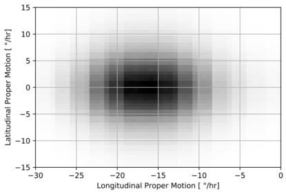
Figure 2: Proper motion distribution used for trajectory priors. This distribution was based on simulating all known objects in the MPC database observable in our survey. It was smoothed using a boxcar filter of width $5\arcsec/hr$ and $9\arcsec/hr$ in latitude and longitude respectively.

3.2 Random trajectories to pixels

In this subsection, we describe the manner in which random trajectories interact with the data in memory. This is a simple approach to efficiently accessing the relevant data in the case where it may all be loaded into random access memory (RAM). We will first describe the approach and then expand on possible extensions to it that could yield the requisite speed-up to make the method more applicable to larger data sets.

We utilized the Flash cluster at Lawrence Livermore National Laboratory (LLNL) employing 2x Xeon E5-2670 v3 (12 cores each) CPUs and 256 GB of SSD memory. This is important to avoid having to access the data through the file system, which adds substantial latency to the queries. This also begins to approximate the requirements for larger survey searches, which will need to be distributed over many nodes of a large high-performance computing (HPC) system. This will add additional challenges such as node to node communication bandwidth and communication cross-linking, which we will discuss in more detail later in this subsection and in §5.

In general, any time-domain survey data may be thought of as filling a three-dimensional space (two spatial and one time), where the units of the two-dimensional spatial domain are pixels covering the two-sphere and the time domain is discretized at irregular steps corresponding to the time of each exposure in the survey. In the linear regime this space may be simplified to a “cube” with square pixels and a short time axis. This assumption allows data collision and lookup indexing to be fast and relatively simple, but is inaccurate over wider surveys and longer periods of time – this is the same challenge that makes traditional shift-and-stack fail beyond a short time regime.

In our case, the survey data set is constructed into this conceptual cube by composing the data space as a three-dimensional stack of layers, with each layer itself being constructed from a series of “tiles” that come from the LSST data processing stack utilized in §2.2. Tiles contain the “real” surface of the data, i.e. the portions which exists somewhere on disk in a FITS file, and each FITS file in the data set is represented as a virtual tile in memory. The FITS files also contain information on the position and size in this global linear coordinate system and that information is used for positioning the corresponding tile within each layer.

The global linear coordinate space is partitioned at each level of the data cube hierarchy. At the top-level, the cube’s two-dimensional projection is the minimum bounding box containing all of the tiles in the reduced data. The layers of the cube can be thought of as the intersection of the cube with parallel planes spaced at the time of each exposure (or perhaps thick planes with thickness corresponding to the exposure time). Each layer shares the same two-dimensional coordinate space (with small differences corresponding to dithering) and differ only in time. Layers also contain information about the length of the exposure represented by the tiles on that layer, so that the flatted two-dimensional footprint of a trajectory’s intersection with the layer can be accurately calculated (this is important for using a proper signal-matched filter later). Tiles have a local coordinate space equal to that of the data array in the FITS file they represent.

Once a random trajectory is sampled, we propagate it through the data cube. At each time where an image exists in the cube, we calculate the trajectory–data cube intersection (in the linear assumption this is trivial), and we pull in the relevant pixel data for the SNR calculation. When looking up pixel data, each level in the cube hierarchy is queried to access the portion of the coordinate stored before moving to the remainder of the query to subordinate levels, if applicable, until the pixel values are fully resolved. All such queries are done by giving the cube object a point in three-dimensional space. First, we determine if the requested position is within the bounding box of the layer and if so, we then determine which layer was requested and pass the remaining two-dimensional query to that layer. We then determine whether or not that point falls within a tile of the layer or within a chip gap or star mask. If the pixel queried exists and contains data, the query is passed to that tile. Once the query reaches the tile, the code retrieves the requested data from its associated FITS file. This is done by renormalizing the requested point to the local coordinate space of the tile and indexing into the data array segment of its associated FITS file to retrieve the requested pixel. A specially encoded NaN value is returned if the requested point cannot be further resolved to a real pixel at any point in this process (e.g., this is the case if the pixel lands in a chip gap or star mask).

In the interest of performance, we did not use any existing FITS library to perform the retrieval of pixel data. Instead, we use Linux’s mmap (or memory map) feature to “map” the primary data array of the FITS file to a 1D array in memory. This provided a number of challenges to overcome but also proved significantly more performant than using, e.g., CFITSIO for this task. The main hurdle for our method was that FITS files store data records in (archaic) spans of 2880 bytes while the memory page size on a typical modern compute sysetm is 4096 bytes, so it is unlikely that the start of a FITS data record will be page-aligned on a modern computer. Linux’s mmap only allows mappings that begin from file offsets that are multiples of the system page size. To work around this, we instead map the offset of the system memory page that contains the start of the data record we are interested in reading and note the difference between the two offsets when performing file accesses. FITS files may also store their data values in different forms of endianness, so we perform an endian swap when reading the pixel data if the endianness of the FITS file does not match that of the system.

3.3 Number of trajectories

Here we estimate the number of required trajectories to satisfactorily cover the space. Following Heinze et al. (2015), the grid space needed to fully sample the proper motion parameters is given by:

$$\Delta=\frac{\sqrt{2}b_{max}}{t_{int}},$$ (2)

where $b_{max}$ is the maximum allowable blur ($\sim 1$ PSF) and $t_{int}$ is the total integration time of the stack (about 100 minutes in our case). Our prior has a radius of $\sim 50\arcsec$ s^-1 in two-dimensional proper motion (Figure 2), so a rough estimate of the required number of trajectories that must be sampled is given by the two-dimensional proper motion domain divided by the square of Eq. 2 multiplied by the number of PSFs in a DECam FOV. This procedure gives $\sim 300\times 10^{9}$. Computing detections for this number of rays took roughly six days on ten nodes of the Flash computing system. In §5 we will discuss improvements to our code that can vastly increase the sampling rate, even with larger data loads and more complex trajectories.

3.4 Signal-to-noise Ratio Calculations

Once the requisite pixels are pulled from the data, the SNR is calculated with a weighted sum using a two-dimensional Gaussian profile convolved with a line segment equal to the length of the expected streak, which we can compute from the sampled proper motion for each trial trajectory (note that for most of the trajectories this is very short, and the convolution reduces to the Gaussian PSF). The flux and noise in each pixel were summed across all images that a given source intersected. Within one image intersection, we measure the flux $F$ by calculating a weighted sum over the pixels $(p)$ inside the streak:

$$F=\sum_{i}{w_{i}*p_{i}}.$$ (3)

The weights $(w)$ are determined from the profile, which is the convolution of a line segment with a two-dimensional Gaussian. The weights are normalized such that their sum equals the effective number of pixels in the streak:

$$n_{eff}=\sum_{i}w_{i}.$$ (4)

The effective number of pixels is calculated by integrating the flux profile:

$$n_{eff}^{-1}=\int{dxdy\,P(x,y)^{2}}.$$ (5)

Specifically, we consider a streak with length $L$ oriented along the x-axis, width $\sigma_{y}$, flux per unit length $l_{0}$, and center (0,0), convolved with a symmetric bivariate Gaussian PSF of width $\sigma_{\pi}$:

$$P(x,y)=\frac{l_{0}}{2L}\frac{1}{\sqrt{2\pi(\sigma_{\pi}^{2}+\sigma_{y}^{2})}}\exp\left(\frac{-y^{2}/2}{\sigma_{\pi}^{2}+\sigma_{y}^{2}}\right)\,\times\\ \left(\operatorname{erf}{\left(\frac{L-2x}{2\sqrt{2\sigma_{\pi}^{2}}}\right)}+\operatorname{erf}{\left(\frac{L+2x}{2\sqrt{2\sigma_{\pi}^{2}}}\right)}\right).$$ (6)

Assuming that the object is unresolved, $\sigma_{\pi}>>\sigma_{y}$, this simplifies accordingly:

$$P(x,y)=\frac{l_{0}}{2L}\frac{1}{\sqrt{2\pi\sigma^{2}}}\exp{\left({\frac{-y^{2}}{2\sigma^{2}}}\right)}\,\times\\ \left(\operatorname{erf}{\left(\frac{L-2x}{2\sqrt{2\sigma^{2}}}\right)}+\operatorname{erf}{\left(\frac{L+2x}{2\sqrt{2\sigma^{2}}}\right)}\right),$$ (7)

where we have defined $\sigma\equiv\sigma_{\pi}$.

We choose an area surrounding the streak to sum over that balances capturing as much signal as possible with limiting computation time. We use twice the full-width-at-half-maximum of the point spread function ($2\sigma$) as a limiting radius away from the streak’s ridge to integrate to, which encompasses over 99 percent of the signal.

Sources of noise include sky background Poisson noise, read noise, dark current, and Poisson noise from the signal itself. The total noise $N$ includes each of these but is dominated by the sources of Poisson noise, which add in quadrature. Thus we have:

$$SNR=\frac{F}{\sqrt{F+N}}.$$ (8)

The background noise is calculated as the standard deviation of pixel values in the difference image. The expected value per pixel will then be the square of this number, and thus we get the total background signal will be:

$$N=\sigma_{\rm pixel}^{2}\,n_{\rm eff}.$$ (9)

All together we have:

$$SNR=\frac{F}{\sqrt{F+n_{\rm eff}\,\sigma_{\rm pixel}^{2}}},$$ (10)

where

$$F=\frac{\sum_{i}{(l_{i}\,p_{i})}\,\sum_{i}{l_{i}}}{\sum_{i}{l_{i}^{2}}},$$ (11)

This is derived from equations 2, 3, and 4, where $l_{i}$ is the formula for the profile and the sums are taken over pixels, which is an approximation for the integral.

3.5 Cuts and Outlier Rejection

Before calculating the overall SNR, some initial filtering is required to deal with potential image artifacts intersected at a small number of exposures. To start, we store a pseudo “light curve” for each trajectory, which is the local SNR on each image the trajectory intersects. Even a few outliers in the light curve can dominate the overall computed SNR for faint asteroids, which are often well below single-epoch detection thresholds, so we apply some outlier rejection methods. We start with a rolling-median sigma clip, and then also apply an overall sigma clip (as opposed to a rolling-median) to trajectories that only intersect 20 or fewer images. We then calculate the total SNR for the remaining unclipped images. We require at least five images intersected and $SNR>5$. After this point, a trajectory is considered a candidate and we store its requisite information: proper motions and intercepts in pixel $(x,y)$ coordinates, overall SNR, and frames intersected. Many of these candidates are false positives or duplicates that are later filtered out.

Next, we apply a filter that removes duplicate detections of the same source. This is a frequent occurrence, especially for bright asteroids because a trajectory that only slightly intersects the deposited flux can quickly surpass the SNR threshold along only a portion of the true trajectory. This filter removes the vast majority of the candidate list. We use a k-d tree to find nearest neighbors for all the trajectories in the four dimensional space of $(x,y)$ position and proper motion (the proper motions are converted to spatial coordinates by multiplying by the total integration time of the data for each night). Using this four-distance metric, we consider all trajectories within $\epsilon=15\arcsec$ of other duplicates. To be explicit, we require:

$$\sqrt{\left(|\vec{x}_{0,i}-\vec{x}_{0,j}|\right)^{2}+\left(\Delta t\,|\vec{\pi}_{i}-\vec{\pi}_{j}|\right)^{2}}<\epsilon,$$ (12)

where $\vec{x}_{0,ij}$ are the position of two trajectories at the first exposure, $\Delta t$ is the time between the last and first exposure, and $\vec{\pi}_{ij}$ are the proper motions.

We keep the trajectory with the highest SNR. We chose $\epsilon=15\arcsec$ as a balance between leaving in too many duplicates and cutting out trajectories that were not duplicates but simply close to each other; 15$\arcsec$ is small enough such that no two known asteroids from the MPC database that are expected to appear in our data are within this range of each other (see Figure 3). It is still likely that some duplicates pass this cut. We address these later.

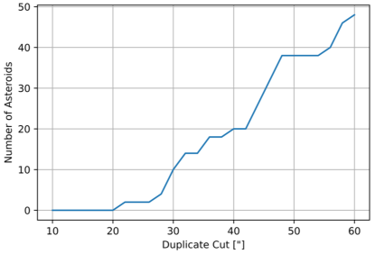
Figure 3: The number of asteroids removed from MPC catalog in our survey as a function of the size of the duplicate cut. No two asteroids are within 20$\arcsec$ in this catalog; there are likely some faint asteroids removed with a cut this large. We use a 15$\arcsec$ duplicate cut in the first step.

We refine each trajectory to more properly align with the source using a Monte Carlo method. This is done by selecting a small postage stamp cutout around each trajectory’s intersection with an image. We then sample $10^{6}$ trial trajectories within these postage stamps centered on the original detection trajectory (specifically, a bi-variate Gaussian of 3$\arcsec$.6 hr^-1 and 2$\arcsec$.6 width along the proper motion and position axes, respectively). We retain the highest SNR trajectory of the sample as the new, refined trajectory. We then apply a second duplicate filter setting $\epsilon=8\arcsec$. Any duplicates that passed the first cut will get closer to each other, and their source, though the refinement process. Thus, the second duplicate process can use a more stringent duplicate cut to successfully filter out almost all remaining duplicates.

Next, we apply a series of filters on the median stack image. This median image is calculated by taking the median across the postage stamp cutouts for each candidate. In this median image, a trajectory that perfectly aligns with a source would appear as a centered single PSF (or short streak for fast moving sources). First we calculate the SNR of this median stack using a weighted sum, and we require $SNR_{med}>7$. Next we apply two filters intended to cut out false positives that are a result of artifacts that survived the difference imaging procedure (typically near bright star masks or the edge of the DECam FOV). First we calculate the noise of the median stack image as the sigma clipped standard deviation of pixel values, and require that it is less than 10 ADU. Next we take all the pixel values outside the source profile and calculate the $\chi^{2}$:

$$\chi^{2}=\frac{1}{N_{pix}}\sum{\frac{p_{i}^{2}}{N_{i}^{2}}},$$ (13)

and require it to be less than 1.5.

Next, we apply a “near-hit” filter that attempts to cut out any trajectory that only partially overlaps with a real source in the data. These are a consequence of under sampling the trajectory priors, especially in the wings of the proper motion prior. We pause here to note that our primary goal is not to optimally detect asteroids in this trial field. We are more interested in developing a framework that may be properly scaled to larger data sets, and we are using this small test survey to being that development. We will return to this discussion in §5. The near-hit filter is carried out by analyzing the distribution of local SNR values in the light curve. For a good hit, most of the local SNR values would distribute around a mean value due to Poisson noise in the flux and the sky background as well as intrinsic variability due to rotation of the asteroid. For a near-hit, the portion of the trajectory that misses the true asteroid motion would exhibit near-zero SNR. To differentiate between these two, we rank-order the local SNR values into an array and compared the standard deviation of the highest values of the distribution (fourth quartile) to the standard deviation of the lowest (first through third quartile). We required that the fourth quartile variance be less than the first through third quartile variance, thus requiring that most of the high value local SNRs are clumped around a value indicative of a detection on all of the frames that intersect the trajectory. We demonstrate asteroids that both pass and fail this cut in Figure 4. In the case where all values are clumped around zero, and this filter is passed, the overall SNR would likely be below our threshold in the first place.

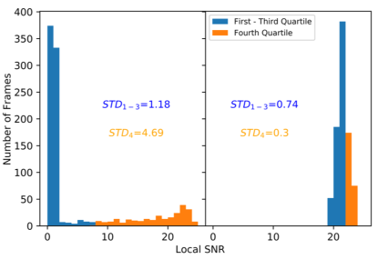
Figure 4: Example distributions of Local SNR values of frames hit for detection trajectories that are bad (left panel) and good (right panel) approximations of the true trajectory. The near hit filter compares the STD of the first through third quartile (blue bins) with the STD of the fourth quartile (orange bins). The near-hit mostly has local SNRs around 0 and some reaching higher corresponding to when the trail trajectory overlaps the flux from the asteroid, and so fails the test. The right panel shows a good hit, which has mostly non-zero local SNRs and passes.

Finally, we also apply a similar filter where we take each trajectory and randomly split its light curve in two. We then require that each half individually must reach the SNR cut of $\frac{5}{\sqrt{2}}$ to check that flux is rougly split between two random halves of the lightcurve.

We then visually inspect each result to remove any remaining false positives or potential duplicates. In figure 5 we demonstrate the overall process as well as the number of detections after each stage for each night.

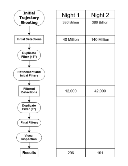
Figure 5: The flow chart for our filtering process along with numbers of detections for each night after every stage. The “Initial Filters” consist of just the median image filters, while the “Final Filters” consist of median image and light curve filters.

4 Results

4.1 Injection and completeness

During data reduction, we injected fake sources into the data to allow us to measure completeness. Roughly 1700 sources were injected each night with uniform distributions of proper motions up to 360$\arcsec$ $\text{hr}^{-1}$ and apparent r-band magnitudes between 18 and 28. We measured completeness by calculating the percentage of injected sources that were detected with respect to both magnitude and proper motion, where the latter is heavily affected by proper motion priors and refinement.

We determined which detections corresponded to injected sources using the same four-distance metric from Eq. 12. For each detection, we found the closest injected source, and if it was within 20$\arcsec$, we considered it a match. We performed a similar analysis on known asteroids in the MPC database. We took all MPC asteroids expected to be within our observations and matched them with a larger minimum four-distance of $70\arcsec$. This was larger to accommodate errors in MPC orbital elements and potential orbit perturbations since last observation. We chose these two four-distance values empirically based on distributions of minimum four-distances, where there was a very clear demarcation between matched and un-matched sources (see Figure 6).

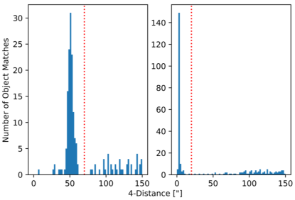
Figure 6: The distribution of four-distances from each detection to the nearest intended matching target (MPC objects on the left panel and injected sources on the right). There is a clear demarcation for each population; the red dotted line shows where we have chosen to separate matches from unmatched objects. These distributions are for night two only and has been cropped to show the small distances. Night one has similar distributions.

In figures 7 and 8, we show completeness along with our proper motion priors. The 5 sigma, single-epoch detection limit was $m_{r}<21.9$ and $m_{r}<21.8$ for nights one and two, respectively. We determined the 5 sigma cuts using the DECam exposure time calculator with a sky background estimated using the model described in Krisciunas & Schaefer (1991), which is derived based on Mie scattering of aerosols and Rayleigh scattering. The Mie scattering term is an empirical fit at large angles though Schaefer (1991) suggests it is valid to within roughly 10^∘ of the moon, which is closer than our fields for each night. The lack of completeness below the red dashed line is suggestive of an incomplete search of the priors, which we mentioned was evident from the large number of near-hits. We again refer readers to §5 on this point, as our main goal of this analysis is to work toward an analysis framework that is scaleable to larger data sets on HPC resources. Indeed, the detections above the red dashed lines in Figures 7 and 8 suggest that the method is working.

In Figure 9, we show completeness specifically for known MPC asteroids. We successfully detect nearly all bright known asteroids and the majority of MPC objects brighter than $m_{V}=21$. These figures display only the detections that are matched with known MPC asteroids, while a substantial fraction of our detections are new.

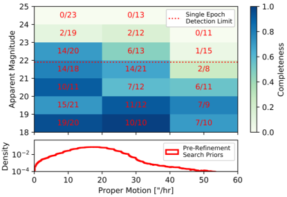
Figure 7: Night one injected source recovery. The red dotted line represents the 5 sigma limiting magnitude for single epoch detection (the limit drops minimally over the x-axis shown). The proper motion priors shown below heavily influence completeness with respect to proper motion. The detection of fast moving objects is a result of imperfect initial detection with possible adjustment with refinement.

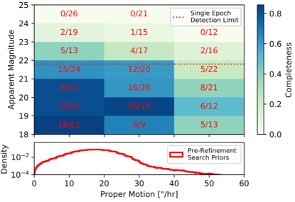
Figure 8: Same as Figure 7 but for night two.

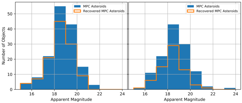
Figure 9: Left: night one recovery of known MPC asteroids. The magnitude distribution of known MPC asteroids in the FOV is shown in solid blue. Those that were successfully recovered are shown in orange. We matched our detections with the known MPC asteroids using the four-distance metric on MPC asteroid positions propagated to the relevant epoch. Right: Same for night two, as with the larger number of false positives, we find that night two was also less sensitive to MPC known asteroids.

4.2 Detections

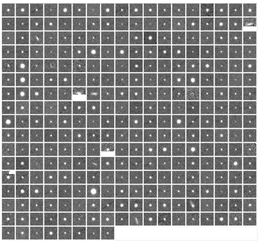
Figure 11: night one detections.

We detected a total of 487 asteroids across both nights, of which 301 are recovered MPC objects. The detections for each night are shown in Figure 10 overlaid on the proper motion prior in log-space to emphasize the tails of the distribution. Two objects detected only in night one where detected in the tails of this prior. A thumbnail of the median stack along the detection trajectory is also presented for each detection for nights one and two in Figures 11 and 12, respectively.

In total, we detected 64 asteroids on both night one and night two. We selected these 64 asteroids by comparing detections across nights and enforcing the same flux was measured and the two detections occurred within $50\arcsec$ of the extrapolated position from the first night detections to the second night. All detections have been reported to the MPC. We present them in Tables 2 and 3. We explored using the rotational reflex velocity (RRV) method to determine these asteroids distances (Heinze & Metchev, 2015; Lin et al., 2016); however, because our observations were not taken near opposition, this method does not provide a one-to-one mapping to distance.

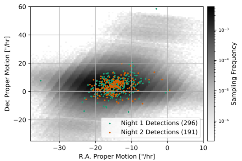
Figure 10: Proper motion of detected asteroids for both nights. The grey scale background shows the proper motion priors used in sampling trajectories. The occasional alignment of dots from each night is the result of detecting the same object across both nights.

5 Discussion

5.1 HPC Considerations

We have alluded to future use cases and extensions for our constructed pipeline throughout this paper, so in the spirit of full specificity, we will discuss the reasons for adopting such a pipeline, the benefits of it, and also the challenges that are unique to this framework.

Between several surveys (past, present, and future) the vast majority of the sky will be observed repeatedly over several decades. Regardless of flux, photons from a large fraction of all asteroids in the Solar System have been deposited in these exposures on hundreds if not thousands of occasions – the vast majority of which may be too faint to detect in single-epoch detection schemes, thus making the embedded information useless for most asteroid detection and linking methods. Accessing this information and combining it to detect more asteroids in a given survey is our fundamental goal. In §3, we laid out the basic idea behind the method. The key features of our method are sampling random trajectories under a prior distribution followed by a finely tuned mapping and gather operation on the data space. The gather operation quickly becomes the bottleneck because a single orbit touches numerous files, which must be accessed separately before the simple requisite computation (e.g., PSF convolution, weighted sum, etc.) can be made. We note here that this challenge is an impediment that traditional shift-and-stack methods do not suffer from because the underlying assumption of linearity ensures that parallel trajectories may always be tested simultaneously via detection on the shifted median stack. Here, we have relaxed the linear assumption and address the I/O challenge head on.

In this paper, to get around this challenge, we used a compute system that was capable of loading all of the requisite data into RAM. We thus avoided latency in accessing the files repeatedly over a file server. In the case where the data load is much larger, this will no longer be possible. A simple mmap implementation becomes much less efficient in the manner we carried out. We are now developing a batched method, which accepts the latency of multiple reads from the file server and instead spends RAM on simultaneous propagation of a larger number of trajectories through time. We have found comparable trajectory sampling rates per node but an ability to scale to arbitrarily large numbers of compute nodes. A follow-on paper will analyze the new implementation performance on a similar data set before we graduate to sampling non-linear trajectories and larger data volumes over longer time domains (Golovich et al. in preparation).

Unfortunately, many of the newest HPC clusters (and more scheduled in the future) do not enable the communication bandwidth to make such a search tractable on large surveys. We must address these issues in order to follow our approach to larger data volumes. As the data volumes grow, the separation of requisite pixels for a given SNR computation grows as well. That is, pixels distributed around an HPC system’s RAM are needed to be combined. In HPC parlance, our code has poor locality. Furthermore, since nearly any number of distinct trajectories touch each pixel, there is a high data access to computation ratio. This tends to add latency in a traditional HPC computation for data fetches. Lumsdaine et al. (2006) describe these types of computational issues for the case of graph algorithms on large data sets, which share many challenges with our vision of a blind asteroid detection pipeline.

Longer time domains also present a new challenge. That is, the search space grows rapidly: a fractional change in orbital elements results in a larger projected, on-sky spatial separation over time. In fact, for large surveys (e.g., Pan-STARRS, ZTF, LSST), the number of possible unique trajectories through the data space becomes exceedingly large.

Despite this search volume problem, the potential to detect extremely faint asteroids remains, so we now explore some of the requirements and challenges posed. Given the immense search space, the most likely use case for a code that can extract detections from a whole survey is in densely searching niche orbital regimes of particular interest such as Earth Trojan asteroids (e.g., Connors et al., 2011) or interstellar objects (e.g., Meech et al., 2017, although we should note that the search space for these is even more immense given the unbounded eccentricity). Under a narrow set of priors for the motion of specific types of objects, an efficient sampling, mapping, and gathering of relevant pixel data from an entire survey could lead to new discoveries. Expanding the discovery space requires optimization of each step (sampling, mapping physical trajectories to the pixel data, and gathering that data). We have shown in this study the importance of optimized loading of data into RAM. In larger surveys, loading all the data into RAM becomes impossible on smaller compute systems, necessitating parallel distributed memory methods, which are foreign to most astronomers. Cutting-edge compute systems have upwards of several petabytes of aggregate RAM, enough to hold even very large surveys; however, accessing this data across many hundreds of compute nodes brings about additional challenges. For one, because an individual orbit may touch hundreds of images across the survey yet those images are distributed through the RAM, there is very little localization. In order to efficiently access the small number of pixels needed to compute the SNR, e.g., an immense amount of cross-talk between compute nodes querying other nodes for their data. These issues will be explored in our future studies.

5.2 Summary

In this paper we motivated and developed a prototype for a new type of blind search for asteroids in astronomical survey data. We provided a proof of concept analysis on a small three hour observation with DECam detecting blindly numerous asteroids fainter than the single epoch depth would permit. We achieve this by parametrizing the motion of asteroids of interest and randomly sampling from prior probability density functions for the motion model and mapping those trajectories to the data space and computing the optimal signal-matched filter for detection. We present the results of our detection pipeline on our test data, finding 487 asteroids with 301 of these matching to known asteroids in the MPC database and 186 being new discoveries. These detections were made despite challenging observing conditions made within $20\arcdeg$ of a nearly full moon. We thoroughly discuss the prospects for such a code in larger surveys and explore the HPC requirements for present and future asteroid surveys.

Figure 12: night two detections.

Table 2: Night One Detections

MPC Designation	$m_{r}$	R.A.	Dec.	$\pi_{\alpha}\cos{\delta}$	$\pi_{\delta}$	Observation Time
	Magnitude	∘	∘	$\arcsec\,hr^{-1}$	$\arcsec\,hr^{-1}$	MJD
	20.21	134.79317	17.34582	57.431	16.524	58475.300347
5512	14.48	134.02066	17.10905	49.997	4.529	58475.300347
	20.75	134.29134	17.63576	56.773	-8.453	58475.301169
326927	18.31	135.53799	17.57403	41.795	-5.965	58475.301169
422173	18.92	134.0232	17.14441	65.643	39.024	58475.300347
377387	19.2	134.71131	16.80628	58.3	28.746	58475.300347
	19.77	134.27197	16.42143	56.311	-4.806	58475.301169
	19.61	135.2303	17.9343	35.45	60.322	58475.300347
	20.19	135.09889	16.94402	66.378	-7.589	58475.300347
	19.05	135.34779	16.84297	34.476	-3.1	58475.300347
	18.0	134.62291	16.47335	11.164	221.666	58475.300347
501015	21.06	135.26071	17.70396	66.039	16.29	58475.300347
100878	17.99	135.14364	16.62999	38.803	26.496	58475.300347
	20.33	134.82584	16.46962	77.055	6.383	58475.300347
	20.36	134.67973	17.80584	48.188	26.118	58475.300347
229604	18.85	135.74152	17.25404	55.572	1.447	58475.300347
	19.51	135.45125	16.83472	31.218	5.512	58475.301169
369867	19.02	135.46566	16.95659	64.4	33.97	58475.300347
501117	20.73	134.42677	16.95386	68.706	15.689	58475.300347
	20.76	135.37694	17.89672	48.122	-6.48	58475.301169
242209	18.01	135.12496	16.23311	75.061	9.547	58475.301169
497263	19.31	134.78628	17.06208	30.148	20.783	58475.300347
42019	17.32	135.57697	17.02326	55.307	17.87	58475.300347
125679	17.26	134.48391	17.87131	61.07	48.136	58475.300347
563034	18.83	135.41812	17.29607	52.998	49.363	58475.300347
62327	17.86	135.19413	17.99334	55.54	27.205	58475.300347
783819	19.49	135.28325	16.90288	50.448	-13.525	58475.300347
99083	18.1	135.94501	16.56385	55.344	-16.92	58475.301169
559253	20.09	135.72067	16.58669	76.843	4.673	58475.301169
315998	19.73	135.56097	16.99877	43.285	21.197	58475.300347
636698	19.84	133.87031	17.0173	50.014	37.303	58475.301968
180367	18.64	135.75742	16.67427	55.399	30.834	58475.300347
199168	18.51	135.82092	17.68091	64.178	-12.744	58475.300347
287521	18.28	135.61687	17.63634	40.531	45.061	58475.300347
320504	18.58	134.23352	16.64174	46.233	-3.2	58475.300347
545217	19.87	134.74767	17.43255	70.063	-10.462	58475.300347
166030	18.21	135.72696	17.19883	43.37	21.078	58475.300347
496976	19.68	134.77711	17.69075	33.327	23.594	58475.300347
110244	18.02	134.92272	17.62696	57.894	23.569	58475.300347
575004	20.22	135.1702	16.49363	68.63	26.687	58475.301968
214124	17.69	135.79507	16.93669	30.802	42.509	58475.300347
350748	17.89	135.40597	17.87755	61.462	-40.19	58475.300347
	19.65	135.70601	17.40023	48.279	13.637	58475.301968
307572	19.43	135.39642	17.39503	44.701	20.88	58475.300347
77485	17.42	135.61702	16.26229	44.789	23.292	58475.301169
321863	18.96	135.68024	17.80152	64.584	35.323	58475.300347
	20.09	135.75291	16.95639	70.368	-31.471	58475.300347
	20.14	135.79085	16.79599	49.26	19.26	58475.300347
	20.29	135.17341	17.07839	66.86	5.108	58475.301169
507022	19.66	134.43732	17.21644	65.624	7.78	58475.300347
48143	17.07	135.02526	17.83662	34.815	51.106	58475.300347
102405	18.16	134.77825	18.03703	54.663	31.115	58475.300347
162069	18.79	134.68747	16.88823	71.141	27.857	58475.300347
	19.96	134.27535	16.95371	56.777	20.66	58475.300347
506183	20.74	134.61118	17.42175	65.341	19.609	58475.300347
254574	18.55	135.79797	17.14525	40.31	24.242	58475.300347
107655	20.34	134.59861	16.16852	56.539	-1.181	58475.300347
173983	17.54	134.91364	17.69367	34.551	36.223	58475.300347
655789	19.69	135.4815	16.84174	59.223	42.707	58475.300347
367784	18.99	134.78362	17.65727	59.545	49.518	58475.300347
724316	20.47	134.76377	16.83589	45.08	7.517	58475.300347
190276	19.56	135.78347	17.03281	68.821	16.402	58475.300347
522895	19.31	135.8193	17.59754	40.039	23.076	58475.300347
745999	18.38	134.47392	17.58256	47.03	8.892	58475.301169
	20.63	135.39451	16.85289	62.923	4.46	58475.300347
474046	19.7	134.59682	17.4886	56.689	15.055	58475.300347
	21.06	134.59864	17.24698	36.805	15.124	58475.301169
429278	19.87	135.71753	17.18038	48.23	28.087	58475.300347
170608	18.78	135.31984	17.33802	53.01	14.767	58475.302766
61818	17.66	134.93991	17.67428	59.961	48.089	58475.300347
	19.52	134.74307	16.2332	41.346	43.186	58475.300347
214666	17.1	135.56074	16.50028	34.317	68.267	58475.300347
125851	18.4	134.8533	16.95914	54.672	35.107	58475.300347
	19.45	134.9119	17.41068	48.654	26.384	58475.301169
120792	18.61	135.43493	17.32942	127.374	29.077	58475.352257
474942	19.74	135.37887	16.29108	50.546	31.295	58475.302766
343950	19.12	135.28006	16.78169	49.698	39.056	58475.300347
373174	19.75	135.92121	17.04615	26.347	28.044	58475.300347
	20.38	135.87684	16.88091	44.222	23.526	58475.300347
273784	19.77	134.04942	17.18428	59.407	13.064	58475.300347
190380	19.62	135.36075	16.11803	30.317	19.31	58475.300347
	19.93	134.55301	16.34607	50.397	29.196	58475.300347
	20.29	134.97073	17.45837	38.634	40.252	58475.300347
	20.49	135.27444	17.38082	58.443	-9.882	58475.300347
509252	20.61	135.85848	16.91407	56.211	17.845	58475.301169
350990	18.34	135.65633	16.96134	32.189	32.944	58475.300347
22308	17.25	136.1153	17.00435	32.55	42.667	58475.300347
456011	19.32	135.09549	17.39107	52.49	-7.736	58475.300347
166530	19.93	135.79449	17.00166	24.684	21.931	58475.300347
	19.83	135.66423	16.56798	52.686	13.334	58475.301169
	19.86	135.43679	17.77679	56.434	-12.992	58475.300347
266184	18.76	134.91723	17.22933	54.472	29.606	58475.300347
	18.45	134.08582	16.68713	54.288	52.081	58475.300347
508023	19.66	135.26764	17.84768	53.882	7.841	58475.300347
	19.64	134.78689	17.34378	49.751	-0.234	58475.300347
	19.21	134.82559	16.5333	59.508	-5.465	58475.300347
178084	19.36	135.84415	16.56622	54.598	17.176	58475.300347
46883	16.7	135.15826	17.73524	61.521	34.949	58475.301169
	20.83	134.10219	17.19007	55.722	-4.338	58475.300347
	19.94	135.7474	16.80471	31.926	15.469	58475.300347
250392	18.1	134.25628	16.49468	55.088	-12.042	58475.300347
9470	15.69	135.69139	17.5841	50.502	10.037	58475.300347
	19.98	135.08763	17.79337	54.468	-2.128	58475.300347
5769	16.55	134.91065	17.49583	55.945	17.863	58475.300347
286186	18.88	135.29339	17.40232	53.641	16.063	58475.300347
	21.01	134.8931	18.00769	1.749	-3.132	58475.301968
	19.27	134.0956	16.93541	76.241	-13.748	58475.300347
17642	17.04	135.23332	17.75534	62.437	33.548	58475.300347
	18.83	135.32308	17.94623	35.372	76.723	58475.300347
220307	18.17	136.09491	16.98661	36.44	-4.09	58475.300347
	17.21	135.54982	17.02742	46.318	19.634	58475.300347
	20.82	135.59494	17.30234	61.552	9.878	58475.300347
300231	18.92	135.28969	16.74339	57.323	8.737	58475.300347
	20.08	135.87517	16.59475	59.324	-24.808	58475.301169
	20.28	135.12598	17.20985	50.76	30.722	58475.300347
	20.29	135.39359	16.3298	43.382	12.798	58475.300347
278673	19.63	134.79528	16.03467	50.989	17.352	58475.301169
188669	19.53	135.40357	18.02587	55.071	22.158	58475.300347
16776	15.68	134.57762	16.06845	33.971	12.496	58475.302766
	20.1	134.0741	16.60081	40.609	29.66	58475.302766
	20.82	135.34161	16.52361	-1.294	3.586	58475.300347
261394	20.37	135.60673	16.52606	49.005	36.634	58475.300347
	19.4	135.94739	17.5561	41.569	42.232	58475.300347
	20.44	134.97392	17.00893	28.638	24.57	58475.300347
77266	17.31	135.12389	16.70643	40.632	19.616	58475.300347
542227	20.58	135.18455	17.41052	57.822	30.258	58475.301968
	20.77	135.23566	17.24622	70.585	7.51	58475.301169
165159	18.23	134.37372	17.14882	63.925	47.412	58475.300347
	20.03	134.51699	17.70129	63.985	-39.287	58475.301169
	20.36	134.81407	17.63194	46.492	0.594	58475.300347
474027	18.87	134.40392	16.64714	52.944	42.167	58475.301968
418129	18.19	134.87483	17.88348	39.931	-18.148	58475.300347
6538	17.25	134.7705	17.12793	66.588	15.804	58475.300347
	20.6	134.48707	17.02795	60.734	31.702	58475.300347
	19.36	135.37545	16.18635	45.609	35.316	58475.300347
260492	17.37	135.49424	16.2389	40.585	-18.641	58475.300347
	19.7	135.34271	16.45115	51.413	-9.634	58475.300347
4443	15.51	134.47003	16.55552	60.06	39.683	58475.300347
488781	20.44	134.31472	16.90327	59.865	29.275	58475.300347
103530	18.55	135.73	17.06041	54.742	14.324	58475.300347
119376	17.49	135.3276	16.49491	41.236	1.555	58475.300347
361051	18.16	134.62338	17.21597	33.166	48.899	58475.300347
	20.78	135.31916	16.59105	54.508	4.007	58475.301169
461884	19.89	135.03417	17.74525	60.311	24.088	58475.301169
	20.66	135.09864	17.62182	37.968	-9.104	58475.300347
	20.45	134.91923	17.66643	72.066	20.606	58475.300347
539738	18.64	134.89698	17.12403	41.935	43.034	58475.300347
	20.66	133.94558	17.13093	58.313	22.471	58475.300347
	19.91	135.1765	17.64411	35.298	27.18	58475.300347
64015	17.44	134.87733	17.90454	54.156	12.55	58475.301169
8978	16.0	135.14704	17.89014	65.675	26.978	58475.300347
423840	19.85	134.46646	16.46711	71.194	29.585	58475.300347
	20.22	134.60573	17.11111	44.773	34.639	58475.300347
147773	19.53	134.80763	17.06768	63.33	19.264	58475.300347
	20.75	135.46048	16.25968	57.169	19.055	58475.301169
661526	19.93	135.77553	16.96214	57.715	1.17	58475.301169
358445	19.35	135.23542	16.63116	47.188	11.246	58475.300347
24761	15.67	135.30375	17.65341	56.99	-18.551	58475.300347
126301	17.2	134.16922	17.22408	40.864	21.326	58475.300347
	20.56	134.37262	17.00279	78.943	-1.699	58475.300347
	20.61	135.50253	17.51833	82.856	-17.575	58475.300347
	17.81	135.91577	16.68033	85.789	-28.674	58475.300347
376906	18.83	134.75587	16.76423	83.931	-52.499	58475.312384
	19.88	135.55198	16.8105	43.921	9.85	58475.300347
183688	18.34	135.57588	16.29158	58.884	24.35	58475.300347
287010	18.24	134.90166	17.88768	53.569	-3.884	58475.300347
	20.19	135.13612	17.81496	52.154	26.939	58475.300347
	20.17	135.3928	16.60968	43.422	16.607	58475.300347
602145	19.84	134.38636	16.55467	58.335	28.688	58475.300347
	20.73	134.83023	18.0493	38.884	-54.864	58475.300347
	19.95	134.73546	16.37383	54.449	3.078	58475.300347
	18.77	135.76502	17.00668	54.048	16.711	58475.300347
255691	19.85	134.25897	16.61406	71.802	19.865	58475.300347
294239	19.51	134.39383	16.54091	60.448	14.357	58475.300347
	18.58	134.57582	16.88552	51.52	-22.064	58475.300347
46837	17.9	135.46872	17.51203	67.994	21.485	58475.300347
	20.15	134.31936	16.90309	68.194	26.618	58475.300347
	20.4	134.5761	17.55046	59.958	-0.076	58475.300347
581272	18.83	135.13438	16.20795	55.833	-15.7	58475.301169
177858	19.63	134.60746	17.35789	60.952	10.915	58475.300347
150968	18.05	134.51746	17.735	50.031	18.05	58475.301169
18668	17.46	134.78653	16.97594	51.23	22.698	58475.301169
217833	19.8	135.83334	16.68884	61.384	27.943	58475.300347
663839	20.47	135.7013	17.22348	60.729	-3.262	58475.300347
	20.87	135.61127	17.78009	60.101	-15.649	58475.300347
417541	18.99	134.55183	17.44795	59.349	29.804	58475.300347
	19.38	135.57666	16.70859	43.738	30.967	58475.300347
	20.74	134.94554	17.95619	44.185	28.296	58475.300347
214491	19.52	134.43224	16.85051	56.798	19.332	58475.300347
	20.37	135.2321	16.33634	39.604	20.264	58475.300347
260657	19.25	135.03231	17.36967	55.331	15.451	58475.300347
	20.5	134.76348	16.10563	77.295	-12.722	58475.300347
552209	19.43	134.60418	16.19545	57.644	5.886	58475.300347
27019	15.41	134.09866	17.39066	52.487	13.752	58475.300347
	19.99	134.52439	17.04456	51.731	12.791	58475.300347
198537	18.37	134.27491	16.53696	62.309	7.164	58475.300347
	19.72	135.91934	17.32968	71.835	-0.475	58475.300347
	20.35	135.35328	17.17408	51.372	24.916	58475.300347
	17.75	135.362	16.11228	67.688	-0.616	58475.300347
205682	17.99	136.1518	16.90252	46.979	-14.569	58475.301169
	20.32	135.19088	17.63654	53.788	4.147	58475.300347
	20.7	134.11844	17.13383	73.308	-7.337	58475.300347
677931	18.88	135.46847	17.37129	39.337	47.97	58475.300347
262895	17.92	134.8744	17.51558	44.239	-3.668	58475.300347
521280	20.02	135.64237	17.05015	49.957	14.994	58475.300347
	17.43	135.02616	17.09924	62.297	14.274	58475.300347
677518	19.1	134.51064	17.13048	47.823	25.56	58475.300347
534631	20.29	134.26493	17.19806	63.942	16.999	58475.300347
9889	16.25	135.67274	17.36914	61.378	23.71	58475.300347
579476	19.58	134.56231	16.97512	27.566	26.953	58475.301968
	18.63	134.62099	16.93608	21.91	33.829	58475.300347
427745	19.54	134.76143	16.15773	70.677	-4.054	58475.300347
	21.02	134.85982	17.50874	59.171	-2.113	58475.301968
	19.78	134.83798	17.27431	33.599	25.769	58475.300347
513029	18.79	135.00649	16.34023	60.03	-3.812	58475.300347
	19.72	135.12797	17.79551	57.816	17.039	58475.300347
230642	18.52	135.44288	16.3727	68.2	5.422	58475.301169
	20.57	135.25256	17.27381	49.12	17.485	58475.300347
	19.8	135.93276	16.62426	72.478	-14.119	58475.300347
391646	19.7	134.94115	16.85069	53.38	17.932	58475.300347
256708	17.67	134.74153	17.02885	18.433	25.373	58475.300347
525327	19.26	134.82291	17.70847	63.129	-7.61	58475.300347
430234	18.66	134.99828	17.53782	76.034	-13.327	58475.300347
673147	19.63	135.8769	16.82667	64.148	2.995	58475.300347
130163	19.15	134.96891	16.84801	59.807	25.06	58475.300347
	19.74	134.84806	16.93507	55.956	31.91	58475.300347
538702	19.58	135.55464	16.4501	56.813	23.288	58475.300347
415273	19.81	135.8166	17.55665	51.653	10.472	58475.300347
148710	18.53	134.72185	16.12625	64.92	13.165	58475.300347
	19.85	135.58038	16.53938	49.747	13.061	58475.300347
	18.35	135.51165	17.31583	49.308	-9.374	58475.300347
	19.51	134.79216	17.22858	49.39	33.797	58475.300347
	20.82	134.09934	17.1773	60.706	-2.61	58475.300347
467952	20.12	134.57006	17.41323	60.037	30.337	58475.301169
	20.14	134.51405	16.12569	49.237	5.602	58475.302766
	20.37	135.76149	17.19018	53.882	9.738	58475.300347
498850	19.19	135.54189	16.95697	46.745	24.606	58475.301968
621143	19.84	134.96609	16.8278	65.547	27.659	58475.300347
	17.8	134.82962	17.84133	56.016	14.378	58475.300347
	19.66	135.2296	16.53891	53.674	20.596	58475.300347
	20.35	134.10112	17.13622	56.182	13.122	58475.300347
	20.54	135.03577	17.10945	62.049	-5.566	58475.301169
	18.41	135.43409	17.3294	46.147	17.276	58475.345914
600245	20.22	134.64215	16.98929	57.779	13.284	58475.300347
318146	19.28	134.52753	17.43151	63.579	3.269	58475.300347
95582	17.56	134.12376	16.6841	53.13	38.164	58475.300347
44014	16.97	135.91186	17.26817	41.452	23.414	58475.300347
	20.77	135.05198	16.69015	36.056	23.54	58475.301968
77420	16.21	135.21516	16.4483	28.509	-19.984	58475.302766
	20.38	134.65146	17.70069	46.886	34.067	58475.300347
463401	19.72	134.70812	17.87152	43.682	36.565	58475.300347
	20.42	135.24513	17.59055	57.772	5.267	58475.300347
472892	19.92	135.66265	16.61926	55.977	29.243	58475.300347
	19.24	135.55943	17.17658	49.82	28.397	58475.300347
255808	17.76	135.54513	17.41992	39.632	33.862	58475.300347
	20.69	134.93874	18.00672	43.501	24.703	58475.300347
216107	20.21	134.59559	17.7875	66.563	21.114	58475.300347
291327	19.23	133.99728	17.00698	64.214	10.35	58475.300347
431811	19.64	135.31303	16.75942	57.649	14.828	58475.301169
	20.17	134.64992	17.1545	45.905	75.348	58475.300347
674128	18.12	134.62777	16.92916	61.382	-43.229	58475.300347
89964	17.36	135.07826	17.18778	47.276	23.893	58475.300347
	19.12	135.24719	16.53393	34.629	18.644	58475.300347
	19.75	134.94336	17.3722	48.585	24.016	58475.300347
	19.29	134.52739	17.42166	60.691	26.028	58475.300347
499477	20.02	135.57338	16.77963	63.713	39.11	58475.300347
	20.5	134.64071	16.93852	34.507	12.726	58475.300347
170158	18.7	134.56489	17.10633	50.193	20.329	58475.302766
	20.13	134.53876	16.29287	26.634	35.057	58475.300347
	20.1	134.38619	16.59145	47.522	14.101	58475.301169
41901	16.72	134.32881	17.61989	43.198	18.792	58475.305961
381522	19.38	135.49721	17.27391	60.77	7.276	58475.300347
100533	17.95	135.11626	16.73943	65.071	21.946	58475.300347
	19.58	134.66398	17.37553	27.568	23.173	58475.300347
	20.27	135.53247	16.92004	53.636	-2.405	58475.301169
352472	18.07	134.05337	17.12481	38.357	72.414	58475.300347
256636	18.28	135.36548	17.93669	60.883	4.316	58475.300347
408797	20.0	134.49007	17.34945	79.785	17.413	58475.300347
	19.76	134.2307	16.55724	37.475	52.787	58475.301169
	20.47	133.97791	17.15478	47.449	-21.524	58475.300347
	20.31	135.3578	16.65846	52.213	29.905	58475.300347
351861	20.18	134.71354	17.27571	62.581	17.24	58475.300347
	18.85	134.27187	16.81163	44.321	54.972	58475.300347
508599	20.03	135.01639	17.48889	75.36	8.471	58475.300347
	20.44	134.61301	17.57297	53.024	21.593	58475.301169
	20.05	135.73037	17.10609	41.069	26.773	58475.300347
215060	18.99	134.82543	16.45099	52.328	21.262	58475.300347
	20.11	135.3333	16.23553	55.839	12.704	58475.300347
	19.94	134.86455	17.59219	46.684	35.15	58475.300347
	20.31	134.91288	17.05437	28.373	24.613	58475.300347
	19.81	134.56303	16.49217	43.829	14.022	58475.301169
381436	20.05	135.22639	17.61307	64.614	19.49	58475.300347
72997	16.69	134.86342	16.48966	51.379	-7.078	58475.300347
107889	16.93	135.51453	17.00693	33.066	48.546	58475.300347
347455	19.3	135.24629	17.80423	51.194	25.297	58475.300347
	20.59	134.27526	16.73583	32.724	0.14	58475.300347

Table 3: Night Two Detections

MPC Designation	$m_{r}$	RA	Dec	$\pi_{RA}\cos{\delta}$	$\pi_{\delta}$	Observation Time
	magnitudes	∘	∘	$\arcsec\,hr^{-1}$	$\arcsec\,hr^{-1}$	MJD
170608	18.63	135.22188	17.36393	55.573	15.898	58476.300833
576938	18.74	136.43999	15.95802	44.19	20.596	58476.302454
	20.06	135.03027	16.6883	36.68	28.919	58476.300833
	19.86	135.8096	17.08086	32.103	19.102	58476.300833
277630	18.92	135.66741	16.22197	42.883	-1.184	58476.300833
341429	18.58	135.79427	15.79003	47.4	23.281	58476.302454
215444	19.65	136.99119	17.07061	63.862	33.106	58476.301655
522895	19.52	135.74501	17.6383	44.641	24.624	58476.300833
	19.59	135.69084	16.83357	35.794	17.402	58476.300833
299971	18.07	135.65043	16.15148	56.851	-9.274	58476.300833
7059	15.24	136.86659	17.06729	48.982	8.442	58476.300833
358445	19.32	135.14534	16.64968	50.581	12.301	58476.300833
111700	17.36	135.93196	16.55727	42.168	29.754	58476.300833
350990	18.88	135.59726	17.01963	35.084	34.42	58476.300833
460720	19.32	135.7289	16.15551	73.714	16.448	58476.300833
177937	18.81	135.68836	15.88187	54.286	13.468	58476.300833
67077	17.41	136.32295	17.19308	69.773	7.776	58476.300833
220480	19.3	136.2989	16.11685	59.96	25.11	58476.302454
214124	17.65	135.74019	17.01302	36.728	43.888	58476.300833
330131	19.43	136.31937	15.79908	63.384	30.625	58476.301655
	20.65	136.67627	16.49828	49.039	18.896	58476.300833
100878	17.78	135.07358	16.67615	44.532	27.266	58476.300833
10054	16.18	136.33663	16.61992	52.22	16.78	58476.302454
118468	17.42	136.51153	16.62008	46.452	26.827	58476.302454
	20.27	136.34698	16.40979	69.765	5.317	58476.302454
198563	18.3	136.33217	16.34901	53.015	13.626	58476.300833
	18.89	135.41844	17.29914	52.348	-8.597	58476.324873
286186	19.03	135.19343	17.42729	56.234	15.854	58476.308854
	20.41	135.31207	16.63987	46.599	19.39	58476.300833
120792	17.65	135.34902	17.37105	50.908	26.273	58476.300833
620113	20.35	136.33872	17.04476	77.986	18.418	58476.300833
	19.23	135.28843	16.83695	38.147	-1.303	58476.300833
77266	17.47	135.05051	16.73986	45.313	20.725	58476.300833
	20.07	135.47953	17.31833	65.547	10.332	58476.300833
99083	17.01	135.86024	16.56101	50.211	0.515	58476.300833
	19.98	135.75424	17.04098	29.064	23.256	58476.301655
308315	19.91	135.33333	16.65702	63.726	9.115	58476.300833
12489	17.32	136.49334	16.071	45.203	14.713	58476.300833
	19.78	135.24967	16.43344	54.615	-8.489	58476.301655
673147	19.65	135.75638	16.83001	68.017	2.912	58476.312106
261394	19.88	135.48795	16.56176	52.07	13.334	58476.301655
410328	18.68	136.00154	16.86384	40.932	21.29	58476.300833
563034	18.95	135.32085	17.38142	54.671	49.993	58476.300833
77422	17.33	136.19751	17.23524	48.395	9.425	58476.300833
504540	19.76	136.40104	17.25066	56.621	11.898	58476.300833
175458	16.44	136.52869	16.5626	46.28	26.737	58476.300833
	20.21	135.76753	16.55105	63.337	-23.436	58476.300833
272748	18.42	136.03915	16.42488	48.578	24.275	58476.300833
11775	17.05	136.25558	16.4975	56.937	16.153	58476.300833
166603	18.37	136.61049	16.28888	57.769	15.102	58476.302454
601077	19.53	136.4359	17.2971	54.517	-5.072	58476.301655
80806	17.07	135.86608	17.7458	48.77	37.85	58476.300833
369867	19.16	135.34519	17.01431	66.979	34.506	58476.300833
263991	17.77	135.71841	15.84891	58.631	38.516	58476.300833
193614	17.7	136.23192	17.71814	39.663	49.021	58476.300833
753413	19.79	136.6366	16.59783	29.121	2.257	58476.300833
	19.17	136.66966	16.83054	54.65	1.386	58476.300833
	19.89	136.34304	16.71795	33.92	30.262	58476.300833
601979	18.24	136.14168	17.22774	55.841	-9.842	58476.300833
233849	19.24	135.88851	16.95816	52.537	17.359	58476.300833
	19.75	136.66689	17.45598	53.062	26.924	58476.301655
	19.39	135.46489	17.22491	52.28	28.865	58476.300833
	20.23	135.65556	17.15474	44.422	29.509	58476.300833
429278	19.42	135.62698	17.22858	51.532	29.027	58476.300833
308359	18.63	135.80359	17.02565	81.777	-20.815	58476.300833
	20.18	135.78246	16.0388	63.717	5.868	58476.300833
127602	17.34	136.2752	16.21634	70.532	2.218	58476.300833
538702	19.71	135.44846	16.48989	59.442	23.436	58476.300833
532854	19.76	136.79087	16.20461	71.127	-6.962	58476.301655
255808	17.72	135.4741	17.47971	45.041	35.759	58476.300833
343388	18.5	135.70054	17.6587	68.257	-11.092	58476.300833
656468	20.32	136.74881	17.0585	52.987	8.986	58476.300833
594360	20.5	136.7577	16.44631	51.739	24.66	58476.302454
277377	19.67	136.32328	17.12817	62.294	22.669	58476.300833
498850	19.13	135.4559	16.99877	50.57	25.117	58476.300833
166030	18.15	135.64987	17.23355	47.223	21.514	58476.300833
473267	18.87	135.81728	17.32215	42.399	49.874	58476.300833
	20.08	136.31433	16.6182	50.547	-0.079	58476.302454
119376	17.26	135.25554	16.49822	43.99	2.772	58476.300833
	19.73	135.61529	17.42385	51.244	14.9	58476.300833
431072	19.47	136.97429	17.05782	43.853	0.713	58476.301655
626709	19.15	135.86705	16.40152	59.217	4.345	58476.301655
663839	20.13	135.58638	17.21575	63.547	-3.197	58476.300833
510285	19.98	135.32888	16.52914	67.827	5.166	58476.301655
365075	18.91	136.48842	16.15177	59.528	10.94	58476.322488
386506	19.27	136.09069	17.75528	46.456	27.302	58476.300833
16500	17.23	136.64005	16.51016	53.986	22.626	58476.300833
	19.8	135.89591	16.90669	61.6	8.903	58476.300833
147181	18.21	136.27812	17.51217	65.831	17.762	58476.300833
324998	18.25	136.69835	16.6882	25.028	-32.699	58476.300833
	19.36	136.24379	16.13965	52.325	22.198	58476.300833
348902	20.05	136.93307	16.53251	39.312	-20.286	58476.302454
491052	18.58	135.972	16.36937	55.269	32.659	58476.300833
42019	17.67	135.47326	17.05354	58.027	18.158	58476.300833
68050	18.01	136.77643	16.49843	76.136	14.782	58476.300833
160942	17.51	135.98831	17.58401	71.649	5.44	58476.300833
9889	15.79	135.55901	17.40975	66.005	25.11	58476.300833
	20.12	135.56822	16.58966	54.599	13.216	58476.300833
503442	19.55	134.97665	16.81495	59.507	5.252	58476.300833
343950	18.84	135.18567	16.84944	53.914	39.654	58476.300833
	20.44	136.15398	17.74642	32.686	6.793	58476.300833
205682	18.07	136.06945	16.87638	52.201	-12.812	58476.300833
	19.63	135.80239	17.77756	-2.331	3.362	58476.308854
	20.6	136.59895	16.5701	70.376	-17.874	58476.301655
	18.86	136.24951	17.03423	67.871	-12.499	58476.300833
211948	18.42	136.31032	17.33449	33.743	10.382	58476.300833
36186	16.65	136.68077	16.10726	49.262	27.374	58476.302454
	20.36	136.17558	16.43811	57.801	17.737	58476.300833
294715	18.65	136.76117	16.21089	61.698	-9.374	58476.301655
214666	17.7	135.49641	16.61914	37.035	69.217	58476.302454
432453	19.17	135.68294	15.83491	47.355	15.379	58476.300833
	17.95	136.48921	16.15486	45.267	-23.018	58476.300833
69945	18.43	135.7733	15.97912	62.584	14.483	58476.300833
327173	18.5	136.99326	16.56207	5.321	31.874	58476.302454
	20.5	135.6533	16.89193	51.873	13.039	58476.300833
9470	15.69	135.59699	17.59959	54.588	10.469	58476.302454
	19.45	135.93277	15.99409	51.228	-27.666	58476.300833
215249	18.56	136.21533	16.1978	67.227	40.871	58476.300833
74196	17.84	136.56215	16.23027	54.267	26.165	58476.300833
	19.48	135.29135	16.24837	48.809	36.925	58476.300833
	19.89	136.13554	16.94882	57.722	8.942	58476.302454
160952	18.12	136.53272	16.7094	74.49	31.54	58476.300833
	19.42	136.61242	17.31761	34.842	-25.805	58476.300833
	20.26	136.63788	16.00316	60.001	-7.2	58476.301655
368106	18.9	136.89205	16.46623	49.552	26.496	58476.300833
	20.27	135.29237	17.13186	49.182	-30.974	58476.301655
	18.5	136.82018	16.52299	51.701	-8.705	58476.3161
661526	20.16	135.66744	16.96293	60.218	2.531	58476.300833
287521	18.31	135.54068	17.71363	43.237	44.68	58476.300833
230642	18.65	135.31528	16.38053	72.082	6.854	58476.300833
97240	16.73	136.01248	16.00087	47.499	6.235	58476.300833
474942	20.2	135.28387	16.34534	54.115	33.091	58476.300833
	20.08	135.84387	16.13753	44.925	21.29	58476.301655
	19.16	136.55238	17.0633	29.329	49.28	58476.300833
180367	18.35	135.65373	16.72844	60.234	32.346	58476.300833
356324	19.36	136.43649	16.72724	46.695	44.309	58476.301655
210410	19.18	136.1321	16.63173	49.737	13.712	58476.300833
334595	19.05	135.61312	17.67213	57.434	17.716	58476.300833
	19.59	135.13039	16.57398	56.332	21.038	58476.300833
	20.35	136.64475	17.03865	50.759	-7.153	58476.300833
	20.27	136.11317	16.54213	49.128	20.527	58476.300833
	20.45	136.29677	17.3111	54.077	18.58	58476.300833
171567	19.05	135.69274	16.19179	71.332	4.918	58476.300833
564072	19.46	136.26338	15.95012	61.111	-16.308	58476.302454
196982	17.73	136.16396	16.57139	49.359	35.86	58476.300833
499477	20.59	135.47242	16.82739	49.813	10.159	58476.300833
	19.5	135.39774	16.84382	35.954	6.016	58476.300833
103530	18.4	135.62942	17.08498	57.766	15.491	58476.300833
139191	18.39	136.44185	16.54856	48.923	23.479	58476.300833
310387	18.42	136.48133	17.72875	39.835	8.064	58476.301655
77420	16.44	135.17018	16.41232	32.634	-20.563	58476.300833
	20.6	136.36311	16.18875	63.489	1.35	58476.300833
	19.35	136.12582	16.95941	45.987	74.678	58476.300833
	18.96	136.29627	15.75668	18.519	31.871	58476.302454
	19.59	135.78388	17.30166	29.191	23.206	58476.301655
208987	17.96	135.78051	16.51568	41.031	22.406	58476.300833
	19.47	136.34439	16.55707	56.927	1.451	58476.300833
141170	18.28	135.83898	16.36287	47.654	23.746	58476.300833
	18.16	136.50655	16.57531	59.82	5.724	58476.300833
210210	19.12	136.4391	15.99642	56.034	11.7	58476.300833
12538	16.32	136.75815	16.15224	51.782	3.636	58476.302454
268038	18.65	136.91207	17.19404	60.57	2.898	58476.300833
18456	15.66	136.47852	17.32713	36.5	14.688	58476.300833
326927	18.26	135.46241	17.5636	47.769	-4.997	58476.300833
	20.28	136.48621	17.23242	60.853	30.47	58476.301655
118976	18.62	136.30441	17.38439	54.625	22.288	58476.300833
83762	16.82	136.59937	16.05942	58.064	-4.025	58476.301655
535650	19.39	135.77725	16.50283	42.691	34.798	58476.300833
	17.8	136.45865	16.60754	50.533	30.287	58476.302454
300100	20.48	135.92023	16.89878	74.564	3.992	58476.300833
422252	19.81	136.49046	16.02948	49.88	30.092	58476.300833
525560	19.87	136.24626	17.75111	53.109	23.285	58476.300833
217833	19.3	135.72047	16.73632	63.379	27.961	58476.300833
62841	17.66	136.67904	16.17763	61.906	10.156	58476.300833
546659	20.46	136.27346	16.68588	66.792	25.52	58476.325683
	20.22	135.21984	16.59767	57.936	5.368	58476.300833
135382	18.37	135.71195	16.19279	62.63	15.304	58476.300833
302010	19.77	134.94177	16.84369	65.979	8.244	58476.300833
	19.7	136.7685	17.13505	30.098	1.39	58476.300833
227354	18.58	136.56422	16.77846	60.666	15.127	58476.302454
	19.8	135.80003	16.59761	74.196	-12.827	58476.300833
	20.68	135.60756	17.34904	53.114	14.332	58476.300833
	19.35	135.19157	16.87652	54.537	-13.032	58476.300833
300231	18.71	135.18482	16.75723	60.001	9.76	58476.301655
677931	18.38	135.39582	17.45446	42.997	49.021	58476.300833
	20.9	135.69761	16.20796	60.43	-8.784	58476.300833
77485	17.29	135.53661	16.30218	48.007	24.638	58476.300833
	19.73	135.78325	17.3273	74.949	0.594	58476.301655
	20.39	136.59471	16.56258	38.316	9.799	58476.301655
	19.61	135.30874	16.15239	34.6	21.38	58476.300833
	19.24	135.5803	17.50614	13.088	51.754	58476.300833

References

- Aihara et al. (2018) Aihara, H., Armstrong, R., Bickerton, S., et al. 2018, PASJ, 70, S8, doi: 10.1093/pasj/psx081
- Aihara et al. (2019) Aihara, H., AlSayyad, Y., Ando, M., et al. 2019, arXiv e-prints, arXiv:1905.12221. https://arxiv.org/abs/1905.12221
- Alard & Lupton (1998) Alard, C., & Lupton, R. H. 1998, ApJ, 503, 325, doi: 10.1086/305984
- Astropy Collaboration et al. (2013) Astropy Collaboration, Robitaille, T. P., Tollerud, E. J., et al. 2013, A&A, 558, A33, doi: 10.1051/0004-6361/201322068
- Astropy Collaboration et al. (2018) Astropy Collaboration, Price-Whelan, A. M., Sipőcz, B. M., et al. 2018, AJ, 156, 123, doi: 10.3847/1538-3881/aabc4f
- Bernstein et al. (2004) Bernstein, G. M., Trilling, D. E., Allen, R. L., et al. 2004, AJ, 128, 1364, doi: 10.1086/422919
- Bosch et al. (2019) Bosch, J., AlSayyad, Y., Armstrong, R., et al. 2019, Astronomical Society of the Pacific Conference Series, Vol. 523, An Overview of the LSST Image Processing Pipelines, 521
- Chambers et al. (2016) Chambers, K. C., Magnier, E. A., Metcalfe, N., et al. 2016, arXiv e-prints, arXiv:1612.05560. https://arxiv.org/abs/1612.05560
- Cochran et al. (1995) Cochran, A. L., Levison, H. F., Stern, S. A., & Duncan, M. J. 1995, ApJ, 455, 342, doi: 10.1086/176581
- Connors et al. (2011) Connors, M., Wiegert, P., & Veillet, C. 2011, Nature, 475, 481, doi: 10.1038/nature10233
- Coupon et al. (2018) Coupon, J., Czakon, N., Bosch, J., et al. 2018, PASJ, 70, S7, doi: 10.1093/pasj/psx047
- Denneau et al. (2013) Denneau, L., Jedicke, R., Grav, T., et al. 2013, PASP, 125, 357, doi: 10.1086/670337
- Flaugher et al. (2015) Flaugher, B., Diehl, H. T., Honscheid, K., et al. 2015, AJ, 150, 150, doi: 10.1088/0004-6256/150/5/150
- Flewelling et al. (2016) Flewelling, H. A., Magnier, E. A., Chambers, K. C., et al. 2016, arXiv e-prints, arXiv:1612.05243. https://arxiv.org/abs/1612.05243
- Granvik et al. (2018) Granvik, M., Morbidelli, A., Jedicke, R., et al. 2018, Icarus, 312, 181, doi: 10.1016/j.icarus.2018.04.018
- Heinze & Metchev (2015) Heinze, A. N., & Metchev, S. 2015, AJ, 150, 124, doi: 10.1088/0004-6256/150/4/124
- Heinze et al. (2015) Heinze, A. N., Metchev, S., & Trollo, J. 2015, AJ, 150, 125, doi: 10.1088/0004-6256/150/4/125
- Heinze et al. (2019) Heinze, A. N., Trollo, J., & Metchev, S. 2019, AJ, 158, 232, doi: 10.3847/1538-3881/ab48fa
- Hunter (2007) Hunter, J. D. 2007, Computing In Science & Engineering, 9, 90
- Ivezić et al. (2019) Ivezić, Ž., Kahn, S. M., Tyson, J. A., et al. 2019, ApJ, 873, 111, doi: 10.3847/1538-4357/ab042c
- Krisciunas & Schaefer (1991) Krisciunas, K., & Schaefer, B. E. 1991, PASP, 103, 1033, doi: 10.1086/132921
- Larson et al. (1998) Larson, S., Brownlee, J., Hergenrother, C., & Spahr, T. 1998, in BAAS, Vol. 30, Bulletin of the American Astronomical Society, 1037
- Lin et al. (2016) Lin, F. R., Peng, Q. Y., Wang, N., et al. 2016, AJ, 152, 183, doi: 10.3847/0004-6256/152/6/183
- Lumsdaine et al. (2006) Lumsdaine, A., Gregor, D., Hendrickson, B., & Berry, J. 2006, Challenges in Parallel Graph Processing
- Masci et al. (2019) Masci, F. J., Laher, R. R., Rusholme, B., et al. 2019, PASP, 131, 018003, doi: 10.1088/1538-3873/aae8ac
- McKinney (2010) McKinney, W. 2010, in Proceedings of the 9th Python in Science Conference, Vol. 445, Austin, TX, 51–56
- McKinney (2011) McKinney, W. 2011, Python for High Performance and Scientific Computing, 14
- Meech et al. (2017) Meech, K. J., Weryk, R., Micheli, M., et al. 2017, Nature, 552, 378, doi: 10.1038/nature25020
- Rein & Liu (2012) Rein, H., & Liu, S.-F. 2012, Astronomy and Astrophysics, 537, A128, doi: 10.1051/0004-6361/2011180
- Schaefer (1991) Schaefer, B. E. 1991, PASP, 103, 645, doi: 10.1086/132865
- Shao et al. (2014) Shao, M., Nemati, B., Zhai, C., et al. 2014, ApJ, 782, 1, doi: 10.1088/0004-637X/782/1/1
- Tyson et al. (1992) Tyson, J. A., Guhathakurta, P., Bernstein, G. M., & Hut, P. 1992, in Bulletin of the American Astronomical Society, Vol. 24, American Astronomical Society Meeting Abstracts, 1127
- Valdes et al. (2014) Valdes, F., Gruendl, R., & DES Project. 2014, in Astronomical Society of the Pacific Conference Series, Vol. 485, Astronomical Data Analysis Software and Systems XXIII, ed. N. Manset & P. Forshay, 379
- Van Der Walt et al. (2011) Van Der Walt, S., Colbert, S. C., & Varoquaux, G. 2011, Computing in Science & Engineering, 13, 22
- Whidden et al. (2019) Whidden, P. J., Bryce Kalmbach, J., Connolly, A. J., et al. 2019, AJ, 157, 119, doi: 10.3847/1538-3881/aafd2d
- Williams et al. (2009) Williams, G., Keys, S., Rudenko, M., & Galache. 2009, Minor Planet Center - Asteroid Orbital Data, VO resource provided by the GAVO Data Center. http://dc.zah.uni-heidelberg.de/mpc/q/pla/info
- Zhai et al. (2019) Zhai, C., Ye, Q., Shao, M., et al. 2019, arXiv e-prints, arXiv:1907.11299. https://arxiv.org/abs/1907.11299
- Zhai et al. (2014) Zhai, C., Shao, M., Nemati, B., et al. 2014, ApJ, 792, 60, doi: 10.1088/0004-637X/792/1/60
- Zhai et al. (2018) Zhai, C., Shao, M., Saini, N. S., et al. 2018, AJ, 156, 65, doi: 10.3847/1538-3881/aacb28