Ensemble Inference Methods for Models With Noisy and Expensive Likelihoods

Abstract

The increasing availability of data presents an opportunity to calibrate unknown parameters which appear in complex models of phenomena in the biomedical, physical and social sciences. However, model complexity often leads to parameter-to-data maps which are expensive to evaluate and are only available through noisy approximations. This paper is concerned with the use of interacting particle systems for the solution of the resulting inverse problems for parameters. Of particular interest is the case where the available forward model evaluations are subject to rapid fluctuations, in parameter space, superimposed on the smoothly varying large scale parametric structure of interest. A motivating example from climate science is presented, and ensemble Kalman methods (which do not use the derivative of the parameter-to-data map) are shown, empirically, to perform well. Multiscale analysis is then used to analyze the behaviour of interacting particle system algorithms when rapid fluctuations, which we refer to as noise, pollute the large scale parametric dependence of the parameter-to-data map. Ensemble Kalman methods and Langevin-based methods (the latter use the derivative of the parameter-to-data map) are compared in this light. The ensemble Kalman methods are shown to behave favourably in the presence of noise in the parameter-to-data map, whereas Langevin methods are adversely affected. On the other hand, Langevin methods have the correct equilibrium distribution in the setting of noise-free forward models, whilst ensemble Kalman methods only provide an uncontrolled approximation, except in the linear case. Therefore a new class of algorithms, ensemble Gaussian process samplers, which combine the benefits of both ensemble Kalman and Langevin methods, are introduced and shown to perform favourably.

60H30, 35B27, 60G15, 82C80, 65C35, 62F15

1 Introduction

The focus of this work is on the solution of inverse problems in the setting where only noisy approximations of the forward problem (the parameter-to-data map) are available and where the evaluations are expensive. The methodological approaches we study are all ensemble based. The take-home message of the paper is that judicious use of ensemble Kalman methodology and generalizations may be used to remove the pitfalls associated with gradient based methods in this setting, but still retain the advantages of gradient descent; the conclusions apply to both optimization and sampling approaches to inversion. We provide theoretical and numerical studies which allow us to differentiate between existing ensemble based approaches, and we propose a new ensemble-based method. Subsection 1.1 provides the set-up in which we work, Subsection 1.2 is devoted to a literature review, while Subsection 1.3 overviews the contributions of the paper and describes its organization..

1.1 The Setting

The problem we study is this: we seek to infer $x\in\mathbb{R}^{d}$ given observations $y\in\mathbb{R}^{K}$ of $G_{0}(x)$, so that

(1) $$y=G_{0}(x)+\xi.$$

The specific instance of the observational noise $\xi$ is not known, but its distribution is; to be concrete we assume that $\xi\sim\mathcal{N}(0,\Gamma)$, with strictly positive-definite covariance $\Gamma\in\mathbb{R}^{K\times K}$. After imposing a prior probability measure $x\sim\mathcal{N}(m,\Sigma)$, application of Bayes rule shows that the resulting posterior distribution is given by

(2) $$\pi_{0}(x) \propto e^{-V_{0}(x)},$$

(3) $$V_{0}(x) :=\frac{1}{2}|y-G_{0}(x)|_{\Gamma}^{2}+\frac{1}{2}|x-m|_{\Sigma}^{2}.$$

This is the standard setting of Bayesian inversion [36]. The objective is either to generate samples from target distribution $\pi_{0}(x)$ (Bayesian approach) or to compute minimizers of $V_{0}(x)$ (maximum a posteriori estimation – the optimization approach). The specific focus of this paper is the setting where $G_{0}(\cdot)$ is expensive to evaluate and only a noisy approximation, $G_{\epsilon}(\cdot)$, is available. The parameter $\epsilon\ll 1$ characterizes the lengthscale, in the space of the unknown parameter $x$, on which the noisy approximation varies.

In order to understand this setting we define

(4) $${G}_{\epsilon}(x)=G_{0}(x)+G_{1}(x/\epsilon).$$

Our goal is to solve the inverse problem (1) defined by $G_{0}$, using only evaluations of $G_{\epsilon}$, not of $G_{0}.$ In this context it is also useful to define the multiscale potential

(5) $$V_{\epsilon}(x):=\frac{1}{2}|y-G_{\epsilon}(x)|_{\Gamma}^{2}+\frac{1}{2}|x-m|_{\Sigma}^{2},$$

and the associated multiscale posterior distribution $\pi_{\epsilon}\propto\exp(-V_{\epsilon})$. Settings in which $G_{1}$ is both random and periodic will be considered. Specifically, we will provide a computational example, arising in climate modeling, of the setting where $G_{1}$ represents random fluctuations caused by finite-time average approximations $G_{\epsilon}$ of the desired ergodic averaging operator $G_{0}$, demonstrating desirable practical performance of ensemble Kalman methods for both Bayesian and optimization approaches in this setting. And, in order to provide deeper theoretical understanding, we will use multiscale analysis to compare ensemble Kalman algorithms and ensemble Langevin algorithms, for solution of the inverse problem (1) where $G_{1}$ is periodic and only evaluation of $G_{\epsilon}$ is possible.

The central message of the paper can now be conveyed by reference to two different classes of stochastic differential equations (SDEs), both defined in terms of $G_{\epsilon}$, but compared on the basis of their ability to solve the inverse problem defined by (1). The first is the ensemble Kalman sampler (EKS) which requires only evaluations of $G_{\epsilon}(\cdot)$. The second is the ensemble Langevin sampler (ELS) which requires evaluations of $V_{\epsilon}(\cdot)$ and its gradient, and hence requires evaluations of the action of the gradient of $G_{\epsilon}(\cdot)$. In both cases the ensemble size is $N$.

The EKS comprises $N$ coupled SDEs in $\mathbb{R}^{d}$, for $X_{t}^{i}$ indexed by $i=1,\dots,N$, and given by

(6) $$\begin{split}dX_{t}^{i}&=-\Bigl{(}\frac{1}{N}\sum_{n=1}^{N}\langle G_{\epsilon}(X_{t}^{n})-\overline{G}_{\epsilon,t},G_{\epsilon}(X_{t}^{i})-y\rangle_{\Gamma}X_{t}^{n}\Bigr{)}\,dt-C_{t}\Sigma^{-1}(X_{t}^{i}-m)\,dt\\ &\hskip 180.0pt\quad\quad\quad+\frac{d+1}{N}(X_{t}^{i}-\overline{X}_{t})\,dt+\sqrt{2C_{t}}\,dW^{i}_{t};\end{split}$$

here the $W^{i}$ are standard independent Brownian motions in $\mathbb{R}^{d}$ and

(7a) $$\overline{X}_{t} =\frac{1}{N}\sum_{n=1}^{N}X_{t}^{n},\qquad\overline{G}_{\epsilon,t}=\frac{1}{N}\sum_{n=1}^{N}G_{\epsilon}(X_{t}^{n}),$$

(7b) $$C_{t} =\frac{1}{N}\sum_{n=1}^{N}\left(X_{t}^{n}-\overline{X}_{t}\right)\otimes\left(X_{t}^{n}-\overline{X}_{t}\right).$$

Thus $\overline{X}_{t}$ denotes the mean of the ensemble $\{X^{i}\}_{i=1}^{N}$, $C_{t}$ is its empirical covariance and $\overline{G}_{\epsilon,t}$ the mean of the image of the ensemble under $G_{\epsilon}.$

Using the same notation $X_{t}^{i}$ for the ensemble members, and for $W_{t}^{i}$, independent Brownian motions in $\mathbb{R}^{d}$, the ELS may be written as, for $i=1,\dots,N$,

(8) $$d{X^{i}}_{t}=-C({X}_{t})\nabla{V}_{\epsilon}({X}^{i}_{t})\,dt+\nabla_{x^{i}}\cdot C({X}_{t})\,dt+\sqrt{2C({X}_{t})}dW^{i}_{t}.$$

Here $C:\mathbb{R}^{Nd}\to\mathbb{R}^{d\times d}$ denotes the empirical covariance function of arbitrary collection of $N$ vectors $\{x^{i}\}_{i=1}^{N}$ in $\mathbb{R}^{d}$ and $X_{t}=\{X^{i}_{t}\}_{i=1}^{N}$.

In the setting where $G_{\epsilon}$ is linear the SDEs defining the EKS and the ELS coincide; they are, however, different from one another in general. Ostensibly, both the EKS and ELS as defined above are targeting the distribution $\pi_{\epsilon}$, however they differ drastically in their behaviour as the small length-scale $\epsilon$ goes to zero. As we shall see, as $\epsilon\rightarrow 0$ the EKS (6) behaves as if $G_{\epsilon}$ were replaced by $G_{0}$ and hence performs well in recovering solutions of the inverse problem (1). In contrast the ELS (8) is dominated by the fluctuations arising from $G_{1}$ and does not perform well in recovering solutions of the inverse problem (1). The EKS effectively denoises $G_{\epsilon}$ whilst the ELS gets stuck in the noise. Motivated by the potential success of the EKS for sampling from models with noisy likelihoods, and by the wish to make controlled approximations of the posterior, we propose here a new class of ensemble method – the ensemble Gaussian process sampler (EGPS) – which can sample effectively from rough distributions without making the ansatz of a Gaussian posterior distribution that is used in the EKS. The strategy underpinning this method involves evolving an ensemble of particles according to overdamped Langevin dynamics using a surrogate GP emulator to replace the noisy, and potentially expensive, log-likelihood term.

The multi-scale analysis and computational experiments that we present lead to an important dichotomy between different classes of ensemble methods which resonates with the conclusions of [57]: (a) those which calculate the gradient of the log-posterior density for every particle within the ensemble and then aggregate this to update the particle positions; (b) those which evaluate the log-posterior for every particle and then compute a gradient, or approximate gradient. We show that those in class b) are robust to the roughness of the posterior landscape and produce approximations of the posterior (2), using only evaluations of $G_{\epsilon}$, but with relaxation times independent of $\epsilon$; in contrast the performance of those in class (a) deteriorates as the characteristic length-scale $\epsilon$ of the roughness converges to zero and do not solve the inverse problem defined by the smooth component $G_{0}$, but rather solve a different inverse problem exhibiting order one corrections.

1.2 Literature Review

The focus of this paper is the solution of Bayesian inverse problems, via optimization or probabilistic approaches. Due to the intractability of the posterior distribution associated to a typical Bayesian inversion problem, sampling methods play an important role in exploring the posterior distribution and providing systematic uncertainty quantification. Due to their wide applicability and practical success, Markov Chain Monte Carlo (MCMC) methods based on Metropolis-Hastings (MH) transition kernels remain the de-facto approach to sampling from high-dimensional and/or complex posterior distributions. Given sufficient computational effort, an MCMC scheme can return an arbitrarily accurate approximation to an expectation of a quantity of interest, however this often requires large numbers of iterations to provide an accurate characterisation of the posterior distribution [22]. For Bayesian models with computationally expensive likelihoods, such as those typically arising in climate modeling [34], the geophysical sciences [51, 9] and agent-based models [27], this may render MCMC based methods computationally prohibitive, as they require at least one likelihood evaluation per MCMC step.

The Ensemble Kalman Sampler (6) is an ensemble-based approach for sampling the posterior distribution associated to a Bayesian inverse problem. It was introduced in [18], without the linear correction term proportional to $d+1$. The linear correction was identified in [47, 19] and ensures that, in the case where the forward map $G$ is linear, the one-particle marginals of the Gaussian invariant measure deliver the solution of the Bayesian linear inverse problem for $G$, subject to additive noise distributed as $\mathcal{N}(0,\Gamma)$ and subject to prior $\mathcal{N}(0,\Sigma).$ In the case where $G$ is linear and when initialized with positive-definite initial covariance $C_{0}$, this system converges exponentially fast, at problem-independent rate, to Gaussian measure given as solution to the linear inverse problem for $G$ subject to additive noise distributed as $\mathcal{N}(0,\Gamma)$ and prior $\mathcal{N}(0,\Sigma)$ [18, 8]. In the nonlinear case, the invariant measure is not known explicitly; however the output of the finite ensemble SDE may be used as a key component in other algorithms for solution of the inverse problem [10, 55] which come equipped with rigorous bounds for the approximation of the posterior.

When the forward map $G$ is differentiable and its derivative can be computed efficiently, then sampling methods which make use of the gradient of the log-posterior density provide means of exploring the state-space effectively. For example, one may consider the overdamped Langevin process [56], given by the solution of the following SDE:

(9) $$dx_{t}=-K\nabla V(x_{t})\,dt+\sqrt{2K}dW_{t}.$$

Here $K$ is symmetric and positive-definite, but otherwise is an arbitrary preconditioner. Under mild conditions [56], the Markov process $(x_{t})_{t\geq 0}$, will be ergodic with unique invariant distribution given by $\pi\propto\exp(-V)$, so that $x_{t}$ will converge in distribution to $\pi$ as $t\rightarrow\infty$. Sampling methods based on discretisations of (9) include the Unadjusted Langevin algorithm (ULA) [61] as well as its metropolized counterpart, the Metropolis Adjusted Langevin Algorithm (MALA) [6], and variants such as the preconditioned Langevin version of the pCN algorithm [11] and the Riemmanian Manifold MALA algorithm (RM-MALA) [23]. Hybrid (also known as Hamiltonian) Monte Carlo based methods also exploit the gradient of $V$ to explore the state-space [12], and have been generalized to the Riemannian Manifold setting in [23]. The Ensemble Langevin Sampler (8) is defined by allowing an ensemble of $N$ copies of (9) to interact through a common preconditioner $C(X_{t})$ depending on the solution of the ensemble of equations. Assuming that $C({X}_{0})$ is positive definite, then $C({X}_{t})$ is positive definite for all $t>0$ and so ${X}_{t}$ converges in distribution to $\overline{\pi}=\pi^{\otimes N}$ [19]. This idea follows from the more general concept of ensemble-based sampling methods which accelerate the Markov chain dynamics by introducing preconditioners computed from ensemble information (e.g. sample covariance) [42, 19, 8, 14]. Since, in the case of a linear forward operator, equation (6) coincides with (8) [18], this connects the ELS with some of the previously cited literature on the EKS. Quantitative estimates on the rate of convergence to equilibrium in the setting of preconditioned interacting Langevin equations can be found in [19, 8].

A number of other ensemble-based sampling methods have been proposed, building on the Ensemble Kalman Sampler and related work. In [55], the authors propose a multiscale simulation of an interacting particle system, which delivers controllable approximations of the true posterior; it is rather slow in its basic form, but can be made more efficient when preconditioned by covariance information derived from the output of the ensemble Kalman sampler. Other such ensemble methods include replica exchange [65, 43] as well as Metropolis-Hastings based approaches [28, 7, 35, 32]. The recent work [45] also employs an ensemble of particles for evolving density estimation using kernel methods with the objective of approximating solution of a Fokker-Planck equation.

The presence of multiple modes in the target posterior distribution is a key cause of slow sampler convergence, as any ergodic Markov chain must spend the majority of its time exploring around a single mode, with rare transitions between modes. Mitigating this issue has various extensions to standard MH-based MCMC including delayed-rejection methods [29, 30], adaptive MCMC and methods based on ensembles to promote better state-space exploration, e.g. parallel tempering [43] and others. This issue is further exacerbated for models with posterior distributions exhibiting “roughness” characterised by a non-convex, non-smooth posterior with large numbers of local maxima, such as inverse problems arising in climate modeling [13], Bayesian models in geoscience [9], frustrated energy landscape models in molecular models of protein structures, glassy models in statistical physics and similar models in the training of neural networks [4]. In the context of Bayesian inverse problems, such pathologies may arise naturally if the forward model exhibits multiscale behaviour [15], particularly when only sparse data is available, giving rise to identifiability issues. Alternatively, this may occur if one only has access to a noisy estimate of the likelihood, e.g. for some classes of intractable likelihoods such as those arising from stochastic differential equation models with sparse observations. Similarly, rough posteriors may also arise if one is fitting a Bayesian inverse problem based on estimators of sufficient statistics of the forward model [46]; this setting arises in parameter estimation problems of the type described in [10], where time-averaged quantities are used for parameter estimation in chaotic dynamical systems. In the special case where one has an unbiased estimator of the likelihood then Pseudo-Marginal MCMC methods [1] provide means of sampling from the exact posterior distribution, but the performance of these methods degrades very quickly with increasing dimension. In the context of uncertainty quantification, Gaussian Processes (GPs) were first used to model ore reserves for mining [40], leading to the kriging method, which is now well established in the geo-statistics community [63]. Subsequently, GPs have been very successfully used to provide black-box emulation of computationally expensive codes [62], and in [37] a Bayesian formulation of the underpinning framework is introduced. Emulation methods based on GPs are now widespread, finding applications ranging from computer code calibration [31], global sensitivity analysis [49], uncertainty analysis [48] and MCMC [41].

Surrogate GP models to accelerate MCMC have been considered before, for example in [41] higher-order derivatives of the log-likelihood required in the calculation of Riemannian Manifold Hamiltonian Monte Carlo were calculated via a GP emulator. Similarly, in [64] a nonparametric density estimator based on an infinite dimensional exponential family was used to approximate the log-posterior and then compute the derivatives required for HMC. Surrogate models to augment existing MCMC methods through a delayed rejection scheme have been considered in [69] for GPs and [67] for neural network surrogates. In the context of ensemble methods there have been a number of recent works which make use of interpolation in reproducing kernel Hilbert spaces (RKHS) for density estimation and/or gradient estimation which are subsequently used to formulate a ensemble sampling scheme [58, 45, 59, 53].

Our analysis and evaluation of the algorithms is based on deploying multiscale methodology to determine the effect of small scale structures on the large scales of interest; in particular we apply the formal perturbation approach to multiscale analysis which was systematically developed in [5], and which is presented pedagogically in [54]. To simplify the analysis we perform the multiscale analysis for mean field limit problems, requiring the study of nonlinear, nonlocal Fokker-Planck equations; previous use of multiscale methods for nonlinear, nonlocal Fokker-Planck equations arising from mean field limits may be found in [26, 25].

1.3 Our Contributions

In this paper we make the following contributions to the analysis and development of ensemble based methods for the solution of inverse problem (1), based on forward model $G_{0}(\cdot)$, given only access to the noisy approximation $G_{\epsilon}(\cdot)$ in the form (4):

• we present a parameter estimation problem from climate modeling which naturally leads to the solution of an inverse problem of the form (2), in which only noisy evaluations of the forward model are available, demonstrating favourable behaviour of ensemble Kalman based methods in a setting where $G_{1}$ is random;

• by means of multiscale analysis in the setting where $G_{1}$ is periodic, we demonstrate that the EKS (6) (which does not use gradients of the forward model) exhibits an averaging property that leads to recovery of the SDEs applied with $G_{1}(\cdot)\equiv 0$;

• in the same multiscale setting, we demonstrate that the ELS (8) (which uses gradients of the forward model) exhibits a homogenization property which causes the algorithm to slow down and recover an SDE different from the one with $G_{1}(\cdot)\equiv 0$;

• we introduce the ensemble GP sampler (EGPS) which combines the benefits of the EKS (averaging out noisy forward model evaluations) with the benefits of Langevin based sampling (exact gradients and exact posteriors), overcoming the drawbacks of the two methods (uncontrolled approximation of the posterior, slow performance in presence of noisy forward model evaluations respectively);

• we employ numerical experiments to illustrate the averaging and homogenization effects of the EKS and Langevin samplers, and to show the benefits of the EGPS.

The paper is organized as follows. Section 2 describes the parameter estimation problem arising in climate modeling that serves to motivate our subsequent analysis. In Section 3 we define the EKS and study its application to noisy forward models by means of multiscale averaging. In Section 4 we define a class of interacting Langevin samplers and study its application to noisy forward models by means of multiscale homogenization. Section 5 introduces the new ensemble Gaussian process sampler. Numerical results for all three methods are presented in Section 6 and concluding remarks are made in Section 7. The appendices contain details of the climate modeling example, and of the multiscale analysis.

2 Motivating Example

We present a specific problem of learning parameters from time-averaged data in an idealized climate model. Subsection 2.1 describes the abstract problem of learning parameters in a dynamical system from time-averaged data; noisy fluctuations are introduced when finite time-averaging is used to approximate a desired but intractable infinite time-average. In Subsection 2.2 this setting is applied to the specific motivating example of learning parameters in a GCM (general circulation model). Subsection 2.3 describes the application of ensemble Kalman methods to solve the problem. The example serves two primary purposes: we provide an explicit instance of a noisy energy landscape $V_{\epsilon}$ and we demonstrate the favourable properties of ensemble Kalman methods when solving optimization or sampling based inverse problems defined by such a landscape. In particular, the random white noise fluctuations that appear in this example provide a severe test of the ensemble Kalman methodology; in this context the results of this section are very positive regarding the performance of ensemble Kalman methods. This motivates the analysis which follows in subsequent sections.

We take great care with our notation in this example. We label the unknown $\theta$ and use $\mathcal{G}_{0},\ \mathcal{G}_{1}$ and $\mathcal{G}_{\epsilon}$ to denote the desired forward model, the random fluctuations about it and the noisy forward model ($\mathcal{G}_{\epsilon}=\mathcal{G}_{0}+\mathcal{G}_{1}$) to which we have access, respectively. We use the calligraphic $\mathcal{G}_{\epsilon}$, rather than $G_{\epsilon}$, to distinguish from the multiscale analysis (in subsequent sections) where the lengthscale $\epsilon$ is precisely defined through periodic fluctuations in parameter space . In what follows, $\mathcal{G}_{\epsilon}$ is subject to white noise, and hence to arbitrarily short lengthscale $\epsilon$ for the fluctuations; in practice, however, a value of $\epsilon$ satisfying $0<\epsilon\ll 1$ can still be defined as the minimal separation between the points in $\theta$-space at which $\mathcal{G}_{\epsilon}$ is evaluated. Therefore $\mathcal{G}_{\epsilon}$ should be understood with such a choice of $\epsilon$ in the random setting.

2.1 Parameter Inference From Time-Averaged Data

Our point-of-departure is the following parameter-dependent dynamical system:

(10) $$\frac{du}{ds} =F(u;{\theta}),\quad u(0)=u_{0}.$$

We assume that this dynamical system is ergodic and mixing. We let $u(t;\theta)$ denote the parameter-dependent solution of this problem. Our goal is to learn $\theta$ from data $y$ computed from finite time-averages of a function $\varphi(\cdot)$, defined on the state space, over time-interval of duration $T.$ In detail we have data $y$ given by

$$y=\mathcal{G}_{\epsilon}({\theta})+\xi_{obs},$$

where

$$\mathcal{G}_{\epsilon}({\theta})=\frac{1}{T}\int_{0}^{T}\varphi\bigl{(}u(s;\theta)\bigr{)}ds,$$

and where $\xi_{obs}\sim\mathcal{N}(0,\Delta_{obs})$ is observational noise. We note that $\mathcal{G}_{\epsilon}$ depends on initial condition $u_{0}$, which we view as a random variable distributed according to the invariant measure of (10). For ergodic, mixing dynamical systems a central limit theorem may sometimes be proven to hold [2], or empirically observed, for data drawn at random from the invariant measure. In this setting

$$\mathcal{G}_{\epsilon}({\theta}) \approx\mathcal{G}_{0}({\theta})+\mathcal{G}_{1}({\theta}),$$

$$\mathcal{G}_{1}({\theta}) \sim\mathcal{N}\bigl{(}0,T^{-1}\Delta(\theta)\bigr{)},$$

where $\mathcal{G}_{0}$ is the infinite time-average which, by ergodicity, is independent of the initial condition $u_{0}$. Thus $\mathcal{G}_{\epsilon}(\cdot)$ may be viewed as a noisy perturbation $\mathcal{G}_{1}(\cdot)$ (with standard deviation scaling with $T^{-\frac{1}{2}}$) of the function $\mathcal{G}_{0}(\cdot)$ where the noise induced by the unknown initial condition $u_{0}$ appears only in $\mathcal{G}_{1}$ and not in $\mathcal{G}_{0}$. Whenever we evaluate $\mathcal{G}_{\epsilon}$ at different $\theta$ this noisy evaluation should be thought of as being evaluated independently with respect to random initial condition $u_{0}.$ Hence, evaluations of $\mathcal{G}_{\epsilon}$ contain rapid fluctuations that are white in $\theta$-space; as mentioned earlier $\epsilon$ can be thought of, in practice, as the minimal separation between $\theta$ values at which time-averages are evaluated.

We approximate $T^{-1}\Delta(\theta)$ by a constant covariance $\Delta_{model}$ estimated from a single long-run of the (ergodic and mixing) model at a fixed parameter $\theta^{\dagger}$ and batched into windows of length $T$. If we let $\xi_{model}\sim\mathcal{N}(0,\Delta_{model})$, and assume that the observation error $\xi_{obs}$ is independent of the initial condition $u_{0}$, then we have inverse problem

(11) $$y=\mathcal{G}_{0}(\theta)+\xi$$

where $\xi=\xi_{obs}+\xi_{model}\sim\mathcal{N}(0,\Delta_{obs}+\Delta_{model}).$ It is then of interest to solve this inverse problem given data $y$ and using algorithms which have access only to (random) evaluations of $\mathcal{G}_{\epsilon}.$

2.2 Parameter Estimation in a General Circulation Model

Climate modeling provides a significant application where the set-up of the preceding subsection is relevant. Whilst numerical weather prediction is entwined with learning the initial condition $u_{0}$ of the system, in the setting of climate modeling $u_{0}$ is a nuisance parameter of no intrinsic interest. It is thus natural to calibrate models to time-averaged data, with goal being the prediction of climate statistics into the future. In this setting it is natural to solve the inverse problem relating to infinite time-averages, since the nuisance parameter $u_{0}$ disappears from this problem, but to do so given only the ability to evaluate finite time-averages, because infinite time-averaging is not feasible in practice.

We consider an idealized moist GCM detailed in [17, 50]. The GCM comprises three space-dimensional time-dependent coupled partial differential equations (PDEs) describing the large-scale atmospheric motions of an aquaplanet, representing conservation of mass, momentum and energy. The PDEs are coupled with parameterizations to resolve the subgrid-scale dynamics, notably of moist convection, turbulence and radiation. In the experiments reported, the GCM has a spherical spectral discretization of (32,64,20) discrete latitudes, longitudes, and vertical layers (unevenly spaced in the vertical, with more discrete layers near the planet surface). The time discretization is based on operator-splitting, combining a leapfrog method (explicit) with a Robert-Asselin time filter (implicit) – a standard approach for spectrally discretized atmospheric models [60, 3, 66] . The simulated aquaplanet is statistically homogeneous in the longitudinal direction, and statistically stationary in time, after an initial burn-in period. The computational experiments with these discretizations are stable, and take approximately 1-2s per simulated day when distributed over 8 CPU cores.

A Bayesian formulation of the inverse problem of learning two subgrid-scale convection parameters, the relative humidity RH and the relaxation time $\tau$ is presented in [13]. The quasi-equilibrium moist convection scheme used to describe subgrid-scale phenomena relaxes temperature and specific humidity towards moist-adiabatic reference profiles with a fixed relative humidity RH. As data we take three longitudinally averaged (due to symmetry) and time averaged climate statistics: free-tropospheric relative humidity, daily precipitation and the probability of 90th percentile precipitation. These statistics are known to be informative about the unknown parameters [16]. Observing these quantities latitudinally and averaging over a window of 30 days, we obtain data in $\mathbb{R}^{96}$. The specific formulation of the model, along with details on how the instance of data $y$ and the covariances $\Delta_{obs}$ and $\Delta_{model}$ are constructed are deferred to Appendix A.

2.3 Ensemble Kalman Algorithms For Parameter Inference

We seek to solve the inverse problem (11) using the ensemble Kalman sampler (EKS) algorithm [18], by evolving a set of $N$ particles $\{\theta^{i}_{t_{n}}\}_{i=1}^{N}$ over a discrete set of algorithmic time steps $0=t_{0}<t_{1}<\ldots$ such that $\Delta t_{n}=t_{n+1}-t_{n}$, to approximate the posterior distribution over $\theta$. Note that we distinguish between the EKS, which is an SDE, and the EKS algorithm, which refers to a discretization of the SDE (6) to obtain an implementable methodology. The mean and covariance under the prior on the unknown parameter $\theta$ are denoted $(m,\Sigma)$. We define $M(t_{n})=\big{(}I+\Delta t_{n}C_{t_{n}}\Sigma^{-1}\big{)}$, where $C_{t_{n}}$ is the empirical covariance of the particles $\{\theta_{t_{n}}^{i}\}_{i=1}^{N}$. We consider the approximate posterior sampling approach proposed in [18] which has the form,

$$M(t_{n})\theta_{t_{n+1}}^{*,i} =\theta^{i}_{t_{n}}+\Delta t_{n}C_{t_{n}}\Sigma^{-1}m$$

(12a) $$\quad\quad+\Delta t_{n}\Bigl{(}\frac{1}{N}\sum_{n=1}^{N}\langle\mathcal{G}_{\epsilon}(\theta_{t_{n}}^{n})-\overline{\mathcal{G}}_{\epsilon,{t_{n}}},y-\mathcal{G}_{\epsilon}(\theta_{t_{n}}^{i})\rangle_{\Gamma}(\theta_{t_{n}}^{n}-\overline{\theta}_{t_{n}})\Bigr{)}$$

(12b) $$\theta^{i}_{t_{n+1}} =\theta^{*,i}_{t_{n+1}}+\sqrt{2\Delta t_{n}C_{t_{n}}}\xi^{i}_{n+1},$$

for $i=1,\dots,20$, where $\xi^{i}_{n+1}\overset{\text{i.i.d}}{\sim}\mathcal{N}(0,1)$, and $\Gamma=(\Delta_{model}+\Delta_{obs})I$, and where $\overline{\theta}_{t_{n}}$ and $\overline{\mathcal{G}}_{\epsilon,{t_{n}}}$ are the ensemble averages of $\{\theta_{t_{n}}\}_{i=1}^{N}$ and $\{\mathcal{G}_{\epsilon}(\theta_{t_{n}}^{i})\}_{i=1}^{N}$, respectively. This is a linearly implicit split-step scheme for the SDE (13), but we do not use the finite system size correction, proportional to $N^{-1}$ and identified in [19, 47], because the effect is small for this example; but it is easily incorporated. We also consider the Ensemble Kalman Inversion (EKI) version of this algorithm in which $M(t_{n})\equiv I$ and the white noise contribution is dropped; this corresponds to time discretization of the ordinary differential equation (ODE) found by dropping the last three terms on the righthand side of (6).

We run both the EKS and EKI from algorithmic time $t_{0}=0$ until (approximately in the EKS case) time $5$. For EKI we use $125$ fixed steps, $\Delta t_{n}=0.04$ for all $n$. For EKS we use an adaptive time-step $\Delta t_{n}$ that takes values $0.011,0.038,0.11$ for $n=0,1,2$, and $\Delta t_{n}\approx 0.1$ for $n\geq 3$; we terminate after 49 iterations. For the EKS we use the simple adaptive time-step $\Delta t_{n}$ proposed for the Ensemble Kalman Inversion (EKI) algorithm in [39], and generalized to the EKS in [18]. We choose $N=20$ and in all our numerical examples we evaluate time-averages with $T=30$ days, the same time-interval used to create the data. An initial ensemble of particles of size 20 is drawn from the prior.

Figure 1: Objective function $V_{\epsilon}$ along a line of $200$ parameter values; we vary one parameters and hold the other fixed at the value found from EKI (at time $5$, and for the run $\Delta t=0.04$). The parameter values used to generate the data realization are shown with a blue dashed line; the mean value of the final EKI iteration is a black solid line. The key observation is that EKI produces excellent minimizers despite the rough energy landscape.

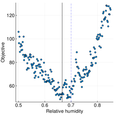
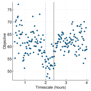
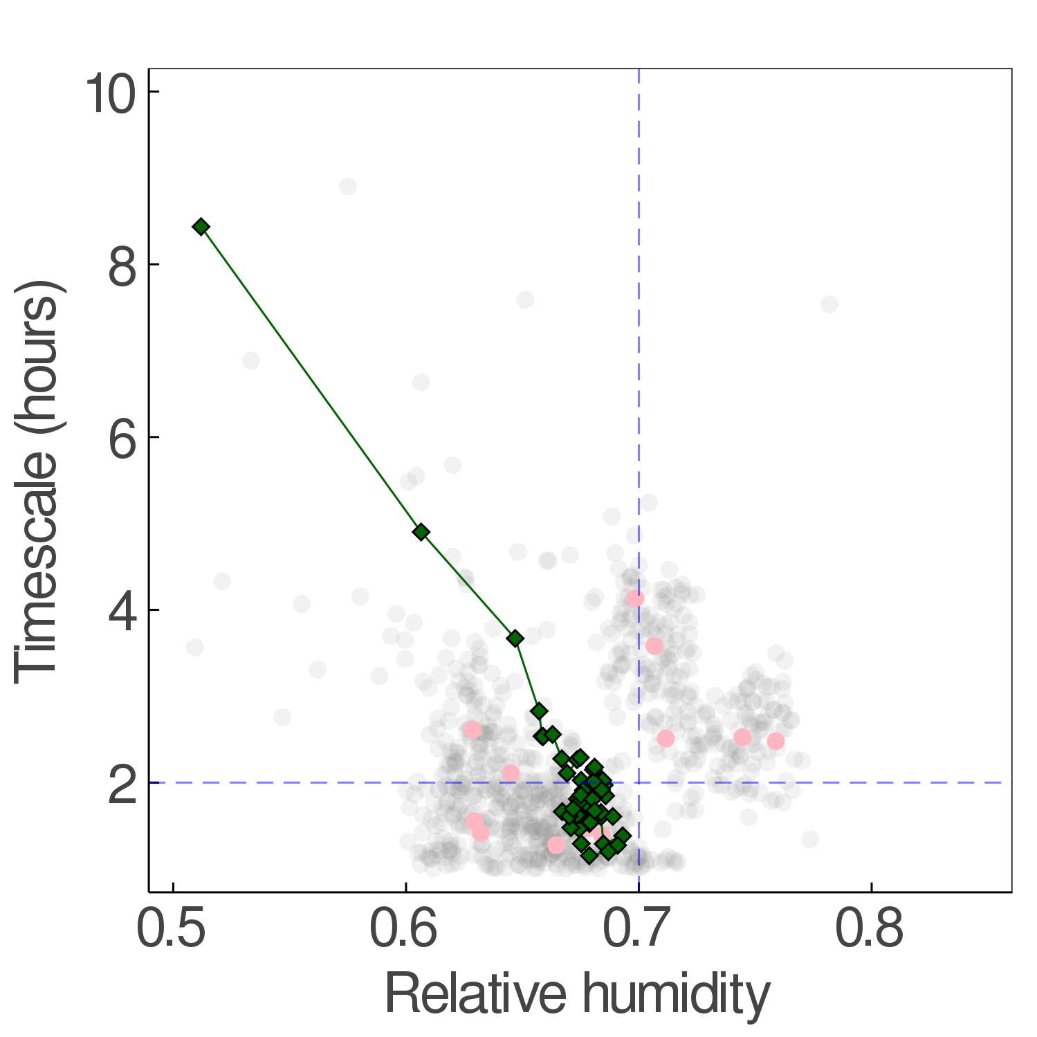
We may now visualize the landscape $V_{\epsilon}$ given by (5) with $G_{\epsilon}$ replaced by $G_{\epsilon}$. Figure 1 shows one-dimensional slices through this landscape; in each we hold one parameter at the optimal value of the objective (taken from the EKI run at time $5$) while varying the other in uniform increments over $200$ values. The objective evaluations (blue circles) are noisy leading to rapid fluctuations around a visible convex objective function (defined by the, in practice uncomputable, infinite time-average limit.) Furthermore the optimal parameter set (black vertical line), defined as the mean of the final iteration of the EKI run at time $t=5$, provides a satisfactory approximate minimizer of the convex objective function buried underneath the noisy objective function constructed from noisy forward model evaluations available to the algorithm; and this is achieved with initialization of the algorithm ensemble from the prior, which is both broad, and far from the truth. The bias of the objective function with respect to the true parameters (blue dashed vertical line) is to be expected, and due to the optimization being performed with a single realization of the noisy data. The behaviour of the EKS algorithm is demonstrated in Figure 2; it too captures the the true parameter very well, despite the noise present in the objective function, and also quantifies uncertainty in the estimate, through the spread of the pink samples.

Figure 2: Convergence of the $20$ member EKS ensemble in parameter space over artificial time 0 to 5 with variable time-step as detailed in the main text. The totality of all ensemble members is shown in grey (noting that some points lie outside of the plotting region). The final ensemble (the $49^{th}$) is given in pink. The parameter set used to generate the data realization is given by the intersection of the blue dashed lines. The green line tracks the ensemble mean over the iterations shown by diamonds. The key observation is that EKS produces excellent samples despite the rough energy landscape.

This ability of ensemble Kalman methods to identify approximate minimizers, and generate approximate posterior samples, in noisy energy landscapes is remarkable. It leads to the conjecture that these derivative-free ensemble methods share a common behaviour of “seeing through the noise” in model evaluations of ${\mathcal{G}}_{\epsilon}$, enabling solution of the inverse problem (11) defined by ${\mathcal{G}}_{0}$. On this basis we will, in the next two sections, compare derivative-free ensemble methods with gradient-based interacting particle systems.

3 Derivative-Free Sampling

The previous section demonstrates that algorithms based on the EKS (6), and its discretizations provide remarkable ability to de-noise rough energy landscapes and identify underlying smooth landscapes relevant for optimization and sampling, in the context of a complex problem arising in climate modeling. In this section we study this problem, returning to the general set-up of the introduction; we work in continuous time and with the superimposed rapid fluctuation in the forward model assumed to be periodic. This simple setting yields clean theoretical insight, and experience from the homogenization and averaging literature [5] suggests that similar results are to be expected for rapid random and periodic fluctuations, and so can provide explanation of the remarkable behaviour observed in the climate modeling example. In Subsection 3.1 we introduce the mean field limit of (6) which is our starting point; Subsection 3.2 is devoted to analysis of this mean-field SDE, using averaging methods, with detailed calculations left for an appendix. The central conclusion from the work in this section is that the EKS recovers solution to the inverse problem defined by $\mathcal{G}_{0}$ when only evaluation of $\mathcal{G}_{\epsilon}$ is available.

3.1 Ensemble Kalman Sampling

Here we study the EKS given by (6) where $G_{\epsilon}$ is defined by (4), and evaluate the relationship of the SDE to the inverse problem for $G_{0}$ defined by (1). Our approach is to apply averaging techniques to the mean field limit of this system. The mean field limit is given by

(13) $$dx_{t}=-\mathcal{F}(x_{t},\rho)\,dt-\mathcal{C}(\rho)\Sigma^{-1}x_{t}\,dt+\sqrt{2\mathcal{C}(\rho)}\,dW_{t},$$

where $W$ is a standard Brownian motion (independent of the initial condition) in $\mathbb{R}^{d}$ and, for density $\pi$ on $\mathbb{R}^{d}$, we define the functions $\overline{\mathcal{X}},\overline{\mathcal{G}}$ and $\mathcal{C}$ of $\pi$, and $\mathcal{F}$ of $(\pi,x)$, by

(14) $$\overline{\mathcal{X}}(\pi) =\int_{\mathbb{R}^{d}}X^{\prime}\pi(X^{\prime})dX^{\prime},\quad\overline{\mathcal{G}}(\pi)=\int_{\mathbb{R}^{d}}G_{\epsilon}(X^{\prime})\pi(X^{\prime})dX^{\prime},$$

(15) $$\mathcal{C}(\pi) =\int_{\mathbb{R}^{d}}\left(X^{\prime}-\overline{\mathcal{X}}(\pi)\right)\otimes\left(X^{\prime}-\overline{\mathcal{X}}(\pi)\right)\pi(X^{\prime})dX^{\prime},$$

(16) $$\mathcal{F}(x,\pi) =\Bigl{(}\int_{\mathbb{R}^{d}}\langle G_{\epsilon}(X^{\prime})-\overline{\mathcal{G}}(\pi),G_{\epsilon}(x)-y\rangle_{\Gamma}X^{\prime}\pi(X^{\prime})dX^{\prime}\Bigr{)}.$$

Here $\rho$ is the time-dependent density of the process, and self-consistency implies that it satisfies the nonlinear Fokker-Planck equation

(17) $$\partial_{t}\rho=\nabla_{x}\cdot\Bigl{(}\nabla_{x}\cdot\bigl{(}\mathcal{C}(\rho)\rho\bigr{)}+\mathcal{F}(x,\rho)\rho\Bigr{)}.$$

It is useful to notice that $\mathcal{C}(\rho)$ depends only on $t$ and not $x$ and that hence we may also write

(18) $$\partial_{t}\rho=\mathcal{C}(\rho):D^{2}_{x}\rho+\nabla_{x}\cdot\bigl{(}\mathcal{F}(x,\rho)\rho\bigr{)}.$$

In equation (17) the outer divergence acts on vectors, the inner one on matrices; in equation (18) the Frobenius inner-product $:$ between matrices is used.
Carrillo and Vaes [8] established stability estimates in the Wasserstein distance for solutions of (17) in case of linear $G$, recovering convergence towards equilibrium results by Garbuno et al, see [18].

3.2 The Small $\epsilon$ Limit

In order to understand the performance of the EKS algorithm when rapid fluctuations are present in the forward model on the EKS algorithm, we proceed to analyze it under the following assumption:

Assumption 3.1.

The forward model (4) satisfies

(19) $${G}_{\epsilon}(x)=G_{0}(x)+G_{1}(x/\epsilon),$$

$G_{0}\in C^{1}(\mathbb{R}^{d},\mathbb{R}^{K})$, $G_{1}\in C^{1}(\mathbb{T}^{d},\mathbb{R}^{K})$ and $\int_{\mathbb{T}^{d}}G_{1}(y)\,dy=0$.    

Here $\mathbb{T}^{d}$ denotes the $d$ dimensional unit torus: $G_{1}$ is a $1-$periodic function in every direction. Although the periodic perturbation is a simplification of the typical noisy models encountered in practice, such as the class presented in Section 2, it provides a convenient form for analysis which is enlightening about the behaviour of algorithms more generally; furthermore the multiscale ideas we use may be generalized to stationary random perturbations and similar conclusions are to be expected [5].

We use formal multiscale perturbation expansions to understand the effect of the rapidly varying perturbation $G_{1}(\cdot)$ on the smooth envelope of the forward model, $G_{0}(\cdot)$, in the context of the EKS, using the mean field limit. To describe the result of this multiscale analysis we define the averaged mean field limit equations, found from (13) and (17) with $G_{1}(\cdot)\equiv 0$ so that $G_{\epsilon}(\cdot)$ may be replaced with $G_{0}(\cdot)$:

(20) $$dx_{t}=-\mathcal{F}_{0}(x_{t},\rho_{0})\,dt-\mathcal{C}(\rho_{0})\Sigma^{-1}x_{t}\,dt+\sqrt{2\mathcal{C}(\rho_{0})}\,dW_{t},$$

with

$$\overline{\mathcal{G}}_{0}(\pi) =\int_{\mathbb{R}^{d}}G_{0}(X^{\prime})\pi(X^{\prime})dX^{\prime},$$

$$\mathcal{F}_{0}(x,\pi) =\int_{\mathbb{R}^{d}}\langle G_{0}(X^{\prime})-\overline{\mathcal{G}_{0}}(\pi),G_{0}(x)-y\rangle_{\Gamma}X^{\prime}\pi(X^{\prime})dX^{\prime}.$$

To be self-consistent the density $\rho_{0}(x,t)\in C\bigl{(}(0,\infty);L^{1}(\mathbb{R}^{d};\mathbb{R}^{+})\bigr{)}$ must satisfy the nonlinear Fokker-Planck equation

(21) $$\partial_{t}\rho_{0}=\nabla_{x}\cdot\Bigl{(}\nabla_{x}\cdot\bigl{(}\mathcal{C}(\rho_{0})\rho_{0}\bigr{)}+\mathcal{F}_{0}(x,\rho_{0})\rho_{0}\Bigr{)}.$$

The following result is derived in Appendix B and it shows that, as $\epsilon\to 0$, equation (17) is approximated by (21).

Formal Perturbation Result 3.1.

Let Assumption 3.1 hold with $0<\epsilon\ll 1$. If the solution of (17) is expanded in the form $\rho=\rho_{0}+\epsilon\rho_{1}+\epsilon^{2}\rho_{2}+\cdots$, then formal multiscale analysis demonstrates that $\rho_{0}$ satisfies (21).

Remark 3.1.

• The result shows that, as $\epsilon\to 0$, the mean field SDE (13), and the nonlinear Fokker-Planck equation (17) for its density, are approximated by the SDE (20), and the nonlinear Fokker-Planck equation (21) for its density. This means that the EKS algorithm simply behaves as if $G_{1}\equiv 0$, and ignores the rapid ${\mathcal{O}}(1)$ fluctuations on top of $G_{0}$; this is a very desirable feature for computations whose goal is to solve the inverse problem (1) defined by $G_{0}$ but where only black box evaluations of $G_{\epsilon}$ given by (4) are available.

• This result is consistent with what we observed empirically in the behaviour of ensemble Kalman based algorithms used to learn parameters in a GCM.

• We choose to formulate this result in terms of the mean field limit because this leads to a transparent derivation of the relevant result. The analysis is cleaner in this limit as it concerns a nonlinear Fokker-Planck equation with spatial domain $\mathbb{R}^{d}\times\mathbb{T}^{d}$; similar results may also be obtained for the finite particle system by considering a linear Fokker-Planck equation with spatial domain $\mathbb{R}^{Nd}\times\mathbb{T}^{Nd}$.

• Rigorous justification of the formal expansion could be approached by using the Itô formula (see Chapters 17 and 18 in [54] for example); the main technical difficulty in this setting is the need to derive bounds from below on the covariance operator, something which is considered in [19] where the finite particle system is proved to be ergodic.

4 Derivative-Based Sampling

We now study the ELS (8) and study its relation to solution of the Bayesian inverse problem defined by (1). In Subsection 4.1 we introduce the mean-field limit of the ELS, which is our starting point; Subsection 4.2 is devoted to analysis of this mean-field SDE, using homogenization methods with detailed calculations left for an appendix. The central conclusion from the work in this section is that, in contrast to the EKS studied in the previous section, the ELS performs poorly at recovering solution to the inverse problem defined by $G_{0}$ when only evaluation of $G_{\epsilon}$ is available.

4.1 Ensemble Langevin Sampling

The mean field limit of the ELS (8) takes the form

$$dx_{t}=-\mathcal{C}(\rho_{t})\nabla V_{\epsilon}(x_{t})+\sqrt{2\mathcal{C}(\rho)}dW_{t},$$

where function $\mathcal{C}(\cdot)$ on densities is as in (15) and $V_{\epsilon}$ is given in (5). By self-consistency, the associated non-linear Fokker-Planck equation for the time-dependent density of the process $\rho\in C((0,\infty);L^{1}(\mathbb{R}^{d};\mathbb{R}^{+}))$ is given by

(22) $$\partial_{t}\rho=\nabla_{x}\cdot\bigl{(}\mathcal{C}(\rho)\left(\nabla_{x}\rho+\nabla_{x}V_{\epsilon}\rho\right)\big{)}.$$

Similarly to the previous section, this may be rewritten as

(23) $$\partial_{t}\rho=\mathcal{C}(\rho):\Bigl{(}D^{2}_{x}\rho+\nabla_{x}\bigl{(}\nabla_{x}V_{\epsilon}\rho\bigr{)}\Bigr{)}.$$

4.2 The Small $\epsilon$ Limit

As an ensemble scheme, the system described by (8) aggregates information from individual particles to obtain a better informed direction in which to explore the posterior distribution. Unlike the EKS, these approaches compute the gradient before aggregating across particles. We show that this causes the resulting sampler to be poorly performed with respect to the presence of rapid fluctuations in the evaluation of the likelihood. The following result is derived in Appendix C. It characterises the evolution of the $O(1)$ leading order term of $\rho$ solving (22). Unlike the setting in the previous section for the EKS, the limit is not the same as the Fokker-Planck equation obtained from applying the ELS methodology to the inverse problem defined by forward model $G_{0}$ with posterior given by (2).

Formal Perturbation Result 4.1.

Let Assumption 3.1 hold with $0<\epsilon\ll 1$. If the solution of (22) is expanded in the form $\rho=\rho_{0}+\epsilon\rho_{1}+\epsilon^{2}\rho_{2}+\cdots$, then formal multiscale analysis demonstrates that $\rho_{0}$ satisfies the following mean field PDE:

(24) $$\partial_{t}\rho_{0}=\nabla_{x}\cdot\left(\mathcal{D}(\rho_{0})\left(\nabla_{x}\rho_{0}+\nabla_{x}\overline{V}\rho_{0}\right)\right),$$

where $\overline{V}=V_{0}-\log Z(x)$, $Z(x)=\int_{\mathbb{T}^{d}}e^{-V_{1}(x,z)}\,dz$ and

$$\mathcal{D}(\rho_{0})=\frac{1}{Z(x)}\int_{\mathbb{T}^{d}}\bigl{(}I+\nabla_{z}\chi(x,z)\bigr{)}^{\top}\mathcal{C}(\rho_{0})\bigl{(}I+\nabla_{z}\chi(x,z)\bigr{)}e^{-V}\,dz.$$

Here $\chi:\mathbb{R}^{d}\times\mathbb{T}^{d}\rightarrow\mathbb{R}^{d}$ is a solution to the following second order PDE in $z$, parameterized by $x$:

$$\nabla_{z}\cdot\left(\mathcal{C}(\rho_{0})e^{-V(x)}(\nabla_{z}\chi(x,z)+I)\right)=0,\quad(x,z)\in\mathbb{R}^{d}\times\mathbb{T}^{d}.$$

Furthermore, for arbitrary $\zeta\in\mathbb{R}^{d}$,

(25) $$\zeta^{\top}\mathcal{D}(\rho_{0})\zeta\leq\zeta^{\top}\mathcal{M}(\rho_{0})\zeta.$$

Remark 4.1.

• The homogenized mean field equations in the $\epsilon\rightarrow 0$ limit describe the evolution of a density $\rho_{0}$ with unique invariant distribution given by $\overline{\pi}(x)\propto\pi_{0}(x)Z(x)$. This invariant distribution will generally not be equal to the invariant distribution $\pi_{0}$, associated with the smoothed inverse problem (1), defined in (2) because of the presence of $Z(x)$. This indicates that using an ensemble of coupled Langevin particles applied with potential $V_{\epsilon}$ derived from the noisy forward problem $G_{\epsilon}$ will not result in an ‘averaging out’ to obtain samples from the posterior of the smoothed inverse problem with potential $V_{0}$ derived from the smooth forward problem $G_{0}$; indeed there will in general be an $O(1)$ deviation from the target invariant distribution.

• A second effect that is caused by the fast-scale perturbation is a slow-down of convergence to equilibrium, specifically (25) implies that the spectral gap associated with the mean field equation (24) will be generally smaller than that associated with the slowly-varying forward operator $G_{0}$.

• The same considerations described in the third and fourth bullets of Remark 3.1 also apply here.

5 The Best Of Both Worlds

In this section we detail a gradient-free ensemble method which makes use of smooth estimates of the log-likelihood over the ensemble of particles to estimate the gradient from the available noisy log-likelihood evaluations. This approximation is then used to evolve each particle forward according to overdamped Langevin dynamics in the implied smoothed potential. The proposed method has the advantage of the EKS (robust to noisy energy landscapes) and of the ELS (works with gradients and provides controllable approximation of the invariant measure). In particular, we expect the convergence to the invariant distribution to be faster compared to EKS to due the exploitation of the approximate gradient, which is insensitive to the local noise-induced fluctuations.

To this end, we model the partially observed potential

$$V_{L}(x)=\frac{1}{2}\langle y-G(x),\Gamma^{-1}(y-G(x))\rangle$$

as a Gaussian process $f\sim GP(0,k)$, where $k$ is an appropriately chosen positive definite kernel on $\mathbb{R}^{d}$. This idea is inspired by the paper [45] which uses a closely related approach, with the goal of approximating solutions to a Fokker-Planck equation. In this work, we choose $k$ to be a Gaussian radial basis function kernel of the form $k(x,y;\lambda,l)=\lambda\exp(-\lVert x-y\rVert^{2}/2l^{2})$, where $\lambda>0$ is the kernel amplitude and $l>0$ is the kernel bandwidth. Given (noisy) evaluations of the potential at the ensemble of points ${X}_{t}=(X_{t}^{1},\ldots,X_{t}^{N})\in\mathbb{R}^{N\times d}$ we seek a function $f$ such that, for some $\sigma>0$,

$$V_{L}(X^{i}_{t})=f(X^{i}_{t})+\sigma\xi^{i},\quad\xi=(\xi^{1},\cdots,\xi^{N})\sim\mathcal{N}(0,I).$$

The corresponding Gaussian process posterior for $f$ has mean function

$$\widehat{V_{L}}\textbf{}(x;\sigma,\lambda,l)=\sum_{i,j=1}^{N}k(x,X^{i}_{t};\lambda,l)K({X};\sigma,\lambda,l)^{-1}_{ij}V_{L}(X^{j}_{t}),\quad x\in\mathbb{R}^{d}$$

and covariance function

$$\gamma(x,y;\sigma,\lambda,l)=K(x,y;\sigma,\lambda,l)-\sum_{i,j=1}^{N}k(x,X^{i}_{t};\lambda,l)K({X};\sigma,\lambda,l)^{-1}_{ij}k(X^{j}_{t},y;\lambda,l).$$

Here $K({X})_{i,j}=\sigma^{2}\delta_{i,j}+k(X^{i}_{t},X^{j}_{t})$. The gradient of the posterior mean is well-defined and given by

$$\nabla\widehat{V_{L}}(x;\sigma,\lambda,l)=\sum_{i,j=1}^{N}\nabla_{x}k(x,X^{i}_{t};\lambda,l)K({X};\sigma,\lambda,l)^{-1}_{ij}V_{L}(X^{j}_{t}).$$

The particles in the ensemble are then evolved forward according to overdamped Langevin dynamics, i.e.

(26) $$dX_{t}^{i}=-\nabla\widehat{V_{L}}\textbf{}(X_{t}^{i};\sigma,\lambda,l)\,dt-\Sigma^{-1}X_{t}^{i}\,dt+\sqrt{2}\,dW_{t}.$$

In simply situations the learned energy $\widehat{V_{L}}$ is updated every time-step. The three hyperparameters $(\sigma,\lambda,l)$ are chosen to reflect the spread and local variation in the data and hence, as the conditioning points are updated, these parameters are also adjusted accordingly. We impose log-normal priors on the amplitude $\lambda$ and observation noise standard deviation $\sigma$ and a Gamma prior on the lengthscale $l$. These prior modeling choices on the hyper-parameters ensure that the posterior mean does not introduce any short-scale variations below the levels of the available data [10, 20, 21]. As is standard in the training of GPs we center and rescale the training data to have mean zero and variance one. To select the hyperparameters we employ an empirical Bayesian approach: we compute the maximum a-posteriori values of the hyperparameters after marginalising out $f$. This entails selecting $(\sigma,\lambda,l)$ which maximise the log marginal posterior,

$$MLP(\sigma,\lambda,l;{X}) \propto\frac{1}{2}\log\sum_{i,j=1}^{N}{\widehat{V_{L}}}(X^{i}_{t};\sigma,\lambda,l)K({X};\sigma,\lambda,l)^{-1}{\widehat{V_{L}}}(X^{j}_{t};\sigma,\lambda,l)$$

$$\quad-\frac{1}{2}\log\det K({X};\sigma,\lambda,l)+\log p_{0}(\sigma,\lambda,l),$$

where $p_{0}$ denotes the prior density over the hyperparameters.

In simulations we employ an Euler-Maruyama discretisation of (26), coupled with a gradient descent scheme for adaptively selecting the hyperparameters. Let $X_{n}=(X_{n}^{1},\ldots,X_{n}^{N})\in\mathbb{R}^{N\times d}$ denote the particle ensemble at time-step $n$. The algorithm for evolving the particles forward to time-step $n+1$ is summarised as follows:

• For $i=1,\ldots,N$:

  • Set $X_{n+1}^{i}=X_{n}^{i}-\Delta t\nabla\widehat{V_{L}}\textbf{}(X_{n}^{i};\sigma_{n},\lambda_{n},l_{n})\,-\Delta t\Sigma^{-1}X_{n}^{i}\,+\sqrt{2\Delta t}\,\xi_{n},$ where $\xi\sim\mathcal{N}(0,1)$ iid.

• Update $(\sigma_{n+1},\lambda_{n+1},l_{n+1})=(\sigma_{n},\lambda_{n},l_{n})+\delta t\nabla_{(\sigma,\lambda,l)}MLP(\sigma_{n},\lambda_{n},l_{n};X_{n+1})$.

In the above $\Delta t$ and $\delta t$ are step-sizes for the Langevin updates and the hyperparameter gradient descent, respectively. The choice of $\Delta t$ and $\delta t$ is problem-dependent. While it is possible it is possible that integration with EGP (and EKS) is stiff during the initial transient phase, this can be remedied by using simple adaptive time-stepping. Moreover, for the EGP we see that one of the effects of the smoothing effect of the kernel is to reduce scale separation within the posterior, thus resulting in less stiff dynamics.

If we are in a situation where evaluating the likelihood is computationally intensive, then we may consider a straightforward modification of these dynamics where time is split into a fixed set of epochs where we keep the same conditioning points within the same epoch, performing several steps of Langevin updates and hyperparameter tuning based on the same conditioning points. This permits effective exploration of the posterior distribution but with a fixed number of log-likelihood evaluations. Note that, while we have based the proposed scheme on an underlying Gaussian process model, the use of other non-parametric regression models would be possible, provided that gradients can be readily computed.

6 Numerical Results

In this section we illustrate the performance of the different methods analyzed or introduced in the preceding three sections, comparing their performance on three different numerical examples. In particular we compare the EKS defined in equation (6), the ELS as defined in equation (8) and the EGPS as introduced in Section 5. Our results show the desirable behaviour of the EKS with respect to its ability to avoid the rapid fluctuations imposed on the smooth parametric structure of interest and rapidly converge to the desired smooth posterior; they show the undesirable slowing down of the ELS, but do not illustrate the modified limiting posterior as their slow performance means that this equilibrium distribution is not reached in a reasonable number of iterations. They also demonstrate that the EGPS has the same quality of performance as the EKS, with further improved rate of convergence in continuous time; however, in the units of evaluations of the (assumed expensive) forward model the EKS may still remain competitive. The three examples considered are a perturbed linear model, in Subsection 6.1, the Lorenz ’63 system with parameter estimation through time-averaged data (as for the GCM) in Subsection 6.2 and a multi-modal example, in Subsection 6.3.

6.1 A Linear Model

As a first pedagogical example we consider solving the inverse problem of the form (1) for a forward map $G_{\epsilon}$ of the form, for $x=(x_{1},x_{2})$,

$${G}_{\epsilon}(x) ={G}_{0}(x)+{G}_{1}(x/\epsilon),$$

(27) $${G}_{0}(x) =Ax,\quad{G}_{1}(x)=\left[\sin\left(2\pi x_{1}\right),\sin\left(2\pi x_{2}\right)\right]^{\top},$$

$$A =\begin{pmatrix}-1&0\\ 0&2\end{pmatrix}.$$

The objective is to recover the posterior distribution associated with “slowly-varying” component of the forward model $G_{0}(x)=Ax$, based on evaluations of the multiscale forward map $G_{\epsilon}$. To this end, we generate observed data $y\in\mathbb{R}^{2}$ for a true value of $x$ given by $x^{\dagger}=(-1,1)$ and observational covariance $\Gamma=\gamma^{2}I$ with $\gamma^{2}=0.05$. We impose a Gaussian prior on the unknown parameter $x$ with zero mean and covariance $\Sigma=\sigma^{2}I$, with $\sigma^{2}=0.05$. In the absence of the multiscale perturbation $G_{1}$ in the forward model, the resulting posterior is Gaussian with mean and covariance given by

$$m_{post}=\left(\begin{matrix}\frac{-1}{1+\sigma^{2}}&0\\ 0&\frac{2}{4+\sigma^{2}}\end{matrix}\right)y,\quad\mbox{ and }\quad C_{post}=\gamma^{2}\left(\begin{matrix}\frac{1}{1+\sigma^{2}}&0\\ 0&\frac{1}{4+\sigma^{2}}\end{matrix}\right),$$

respectively. Setting $\epsilon=0.1$, each of the the three methods is used to evolve an ensemble of $1000$ particles from a $U[0,1]^{2}$ initial distribution, over a total of $10$ time-units. The step-size employed for each method is selected differently to ensure stability.

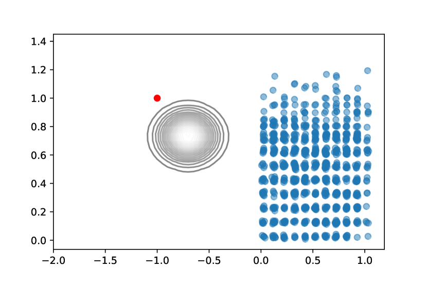
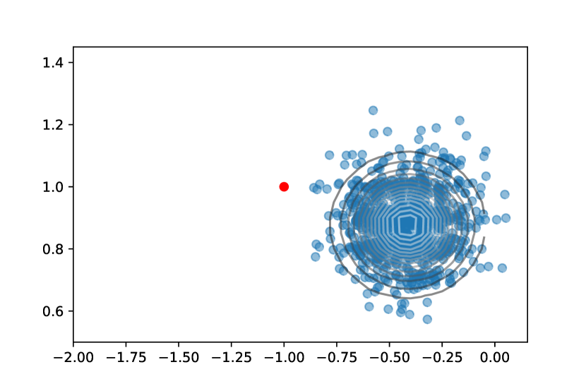
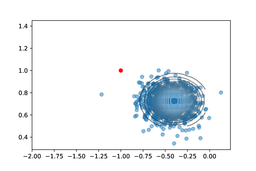
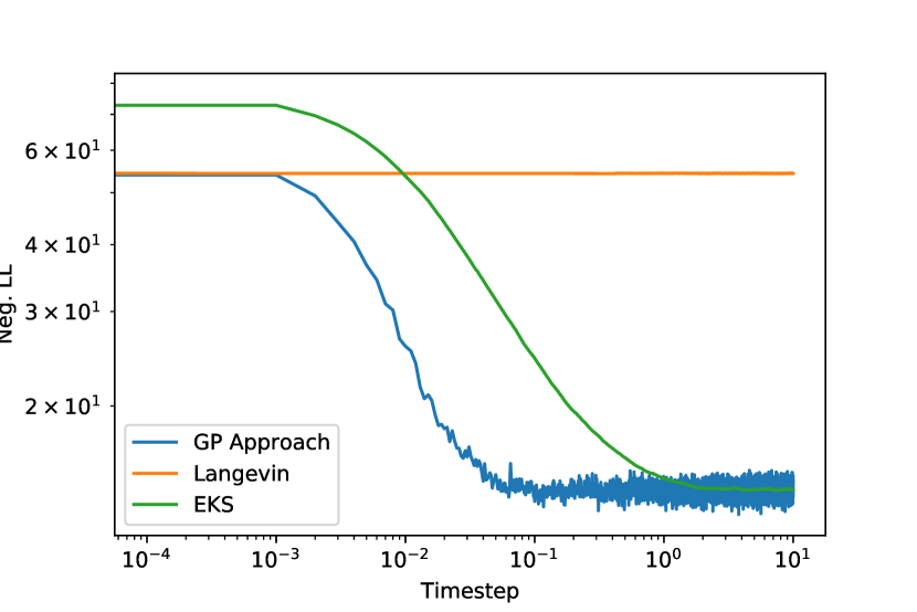
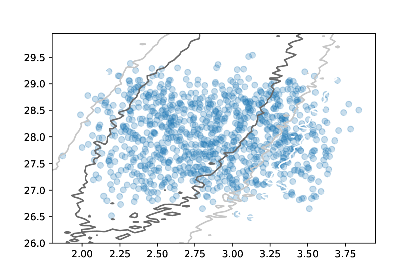
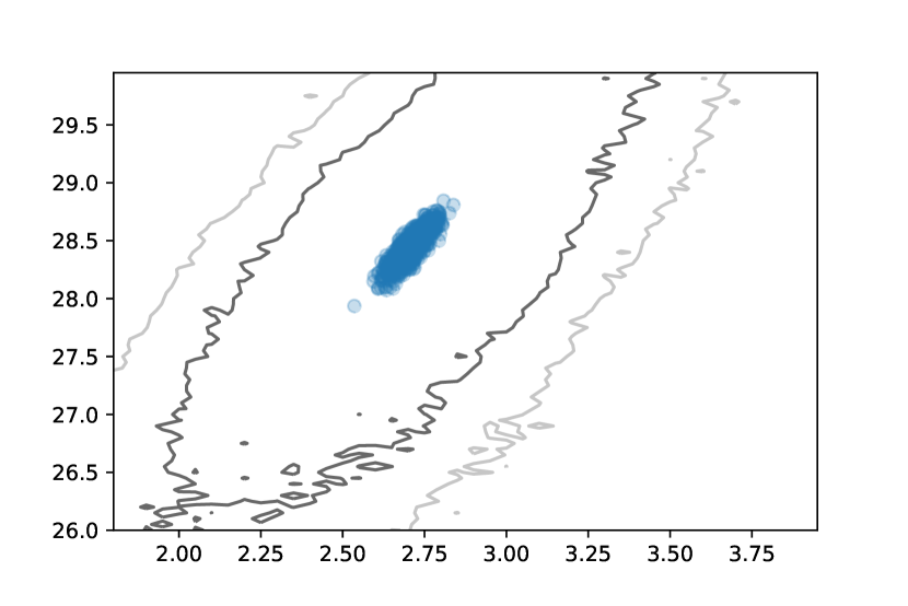
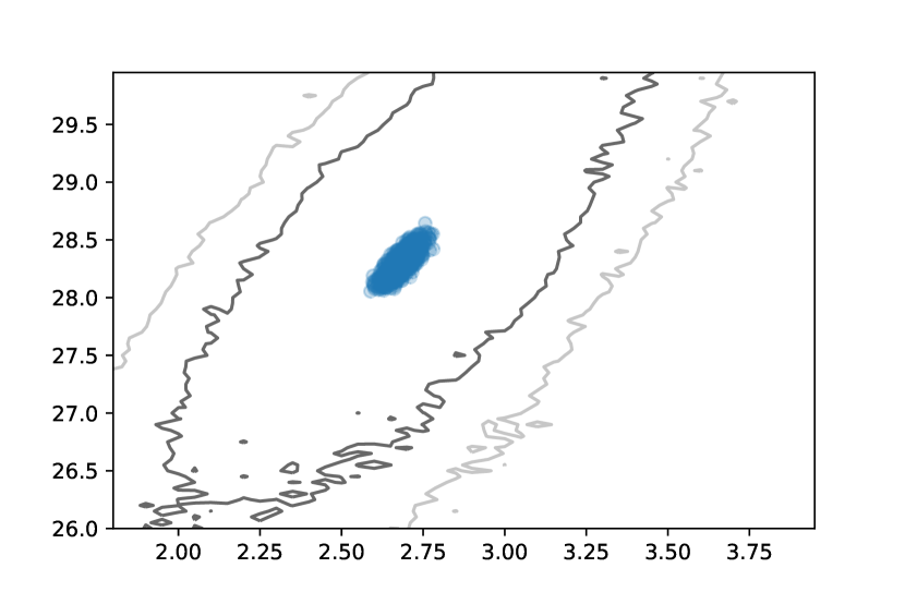
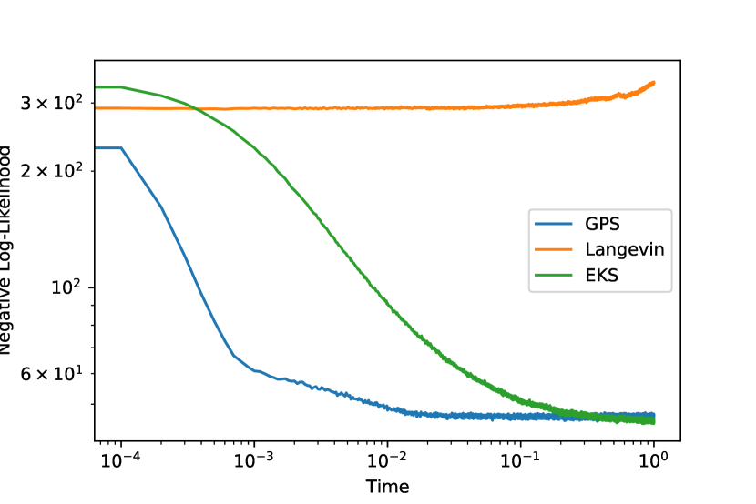
Figure 3 shows the particles ensemble at the final time (blue), the true solution (red dot) as well as the posterior $\pi_{0}$ (2) associated with the slowly varying part of the forward model $G_{0}$ (black contour lines). We observe that particles get stuck in the many local minima for the ELS, shown in Figure 3(a). This is consistent with the Formal Perturbation Result 4.1, which indicates that the multiscale perturbation will slow down the dynamics and will result in a significant deviation of the invariant measure of the SDE from the case $G_{1}=0$. This is not the case for both the EKS and EGPS, which are able to recover the slowly varying target distribution correctly, see Figure 3(b) and Figure 3(c) respectively. Figure 3(d) shows the negative log-likelihood for $\mathcal{N}(m_{post},C_{post})$ averaged across all the particles in the ensemble, as the algorithm progresses. Both the EKS and EGPS rapidly move towards the mode of the slowly-varying target distribution, with the EGPS converging faster due to the use of the approximate gradient. On the other hand the Langevin sampler is strongly influenced by the multiscale perturbations, and after $10$ time units remains distant from the desired Gaussian posterior distribution, stuck in local minima caused by fluctuations $G_{1}.$ While the EGPS converges the fastest, it is sensitive to the initial selection of hyper-parameter values and step-sizes; these were initially set through a preliminary tuning phase for the displayed results. On the other hand, the EKS is remarkably robust to the choice of step-size.

(a) Ensemble Langevin Sampler

(b) Ensemble Kalman Sampler

(c) Ensemble GP Sampler

(d) Negative Log-Likelihood

Figure 3: Plot of the particle ensemble for each of the three processes after simulating $10$ time units. The contour plot indicates the posterior distribution for the “slowly-varying” forward model. The red dot denotes the truth. Note the different scaling of the axes in plots (a-c). The bottom left plot shows the evolution of negative log likelihood as a function of time-step.

6.2 The Lorenz-63’ model

Here we work in the setting of parameter inference from time-averaged data, introduced in Subsection 2.1. Rather than work with the complex GCM studied in Section 2, we work with the Lorenz ’63 model in order to present controlled experiments at cheaper cost.

The 3-dimensional Lorenz equations [44] are given in the form

(28a) $$\dot{x}_{1} =\sigma(x_{2}-x_{1})$$

(28b) $$\dot{x}_{2} =rx_{1}-x_{2}-x_{1}x_{3}$$

(28c) $$\dot{x}_{3} =x_{1}x_{2}-bx_{3},$$

with parameters $\sigma,\,r,\,b\in\mathbb{R}_{+}$. In the following we fix the parameter $\sigma=10$ and focus on the inverse problem of identifying $r$ and $b$ from time-averaged data. To this end, we impose a multivariate log-normal prior on $\theta=(r,b)$ with mean $m=(3.3,1.2)$ and covariance $\Sigma=\text{diag}(0.15^{2},0.5^{2})$; to be concrete this defines the prior distribution satisfied by $\log(\theta)$.

In the notation of Subsection 2.1 we take $T=10$ and define $\varphi\colon\mathbb{R}^{3}\rightarrow\mathbb{R}^{9}$ given by

$$\varphi(x)=(x_{1},x_{2},x_{3},x_{1}^{2},x_{2}^{2},x_{3}^{2},x_{1}x_{2},x_{2}x_{3},x_{1}x_{3});$$

this defines forward model $\mathcal{G}_{\epsilon}$ as a time-average of first and second moments of the solution over $10$ time units. In the experiments that follow data $y$ is found simply from a single evaluation of the random (with respect to initial condition) function $\mathcal{G}_{\epsilon}$.

Data is generated for the parameter set $(\sigma,r^{\dagger},b^{\dagger})=(10,28,\frac{8}{3})$, for which system (28) exhibits chaotic behavior. Matrix $\Delta_{obs}$ is set to zero. We estimate $\Delta(\theta)$, with a matrix $\Delta_{model}$ computing a single long trajectory of (28) at $\theta^{\dagger}=(r^{\dagger},b^{\dagger})$, over $360$ time units. This is split into windows of size $10$ (neglecting the first $30$ units) and we set $\Delta_{model}$ to be the empirical covariance of $\mathcal{G}_{\epsilon}(\theta^{\dagger})$ over the windows.

We then solve the inverse problem using the time discretization of the EKS SDE (6). To ensure that there is minimal correlation between subsequent evaluations of the forward map, we set the initial condition of (28), at each step of the sampling algorithm and for each ensemble member, to be the state of the dynamical system from the previous ODE solve, for the same ensemble member, evaluated at a large random time $t\gg 10$.

Given observation data $y$ and noisy forward model $\mathcal{G}_{\epsilon}$ we define the negative log-likelihood function

(29) $$V_{L}(\theta):=\frac{1}{2}\langle(y-\mathcal{G}_{\epsilon}(\theta)),\Delta_{model}^{-1}(y-\mathcal{G}_{\epsilon}(\theta))\rangle.$$

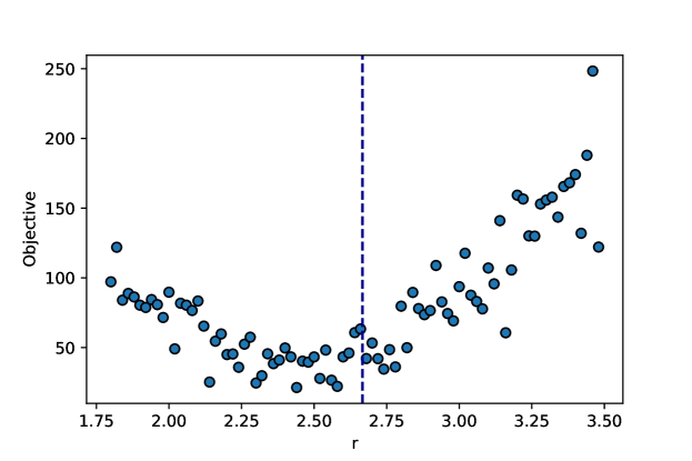
Figure 4 shows the profile of $V_{L}$ versus $r$, for a fixed (truth) value of $b=28$. We denote by $V(\theta)$ the negative log-posterior density found by adding the prior quadratic form to $V_{L}.$

Figure 4: Profile of the noisy negative log-likelihood over $r$ for $b$ fixed at optimal value. The blue dashed line denotes the ’true’ value $r=8/3$.

The EKS, ELS and EGPS processes were all simulated for one algorithmic time unit, with the step-size adjusted to ensure process stability. Each process is simulated with $N=10^{3}$ particles, with initial condition distributed as $U([27,29]\times[2.25,3.5])$. In Figure 5a)-c) we plot the particle ensemble at the final time for each method, overlaid with a contour plot of the negative log-posterior density $V(\theta)$. In Figure 5d) we plot the negative log-likelihood function averaged over the finite-time ensemble for each process, as the algorithms progress. It is clear from the plots in Figures 5 that the EKS and EGPS have concentrated around the true value and are distributed according to a smoothed version of the posterior. On the other hand, the particles undergoing ELS dynamics remain trapped around the local minima of the multiscale posterior distribution, preventing the particles from concentrating in a similar fashion; indeed the ELS is visibly close to the initial (uniform on a rectangle) distribution of the ensemble.

In summary the results of this subsection, where the forward model is random, closely mirror those from the previous subsection, where the forward model is periodic. This substantiates our claim that the analysis of the periodic case, contained in Sections 3 and 4 is informative beyond the confines of the theory.

(a) Ensemble Langevin Sampler

(b) Ensemble Kalman Sampler

(c) Ensemble GP Sampler

(d) Negative Log-Likelihood

Figure 5: The true parameter value is $\theta=(r,b)=(28,8/3).$ Comparison of ELS, EKS and EGPS after simulating the ensemble for $1$ unit of time. The contour plot indicates the posterior distribution $V(\theta)$ while the dots denote the ensemble at the final time. The bottom right plot shows the evolution of negative log likelihood as a function of time.

6.3 Multi-Modal Posteriors

It is well-known that multi-modal posteriors pose a significant challenge for ensemble Kalman-based approaches, since such approaches are constructed using a Gaussian ansatz. Recent work on ensemble-based interacting particle systems in [59] has shown the potential for designing new interacting particle systems which address this multi-model challenge; these methods are based on approximating nonlinear Fokker-Planck equations arising from mean-field dynamics, by means of particle based RKHS methods. In the following we illustrate that, unsurprisingly, the EGPS can achieve similar success, since it is follows similar principles to those underlying the work in [59].

We consider the inverse problem for the form (1) for the unknown parameter $x\in\mathbb{R}^{2}$ given a multiscale forward map of the form $G_{\epsilon}$ defined, for $x=(x_{1},x_{2})$, by

(30a) $$G_{\epsilon}(x) =G_{0}(x)+G_{1}(x/\epsilon),$$

(30b) $$G_{0}(x) =(x_{1}^{2}-1)^{2}+(x_{2}^{2}-1)^{2},\quad G_{1}(x)=\nu(\sin(2\pi x_{1})+\sin(2\pi x_{2})),$$

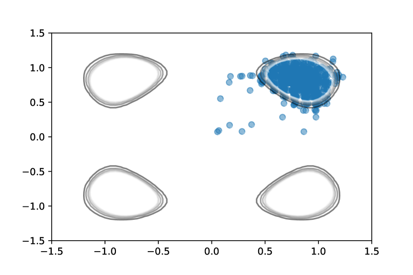
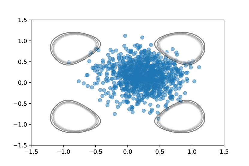
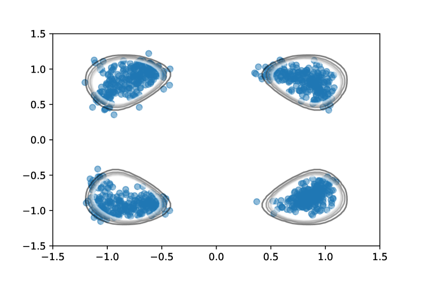
and where $\Gamma=\gamma^{2}I$. To demonstrate the three proposed methods we generate observation data $y\in\mathbb{R}$ for the truth $x^{\dagger}=(+1,-1)$, where $\nu=\frac{1}{10}$ and $\gamma^{2}=0.05$. We impose a Gaussian $\mathcal{N}(0,\sigma^{2}I)$ prior on the unknown parameter $x$, where $\sigma^{2}=0.1$. As the slowly-varying component of the forward map is the non-injective function $G_{0}(x)=(x_{1}^{2}-1)^{2}+(x_{2}^{2}-1)^{2}$, the associated posterior density exhibits $4$ global modes. The ELS, EKS and EGPS were each simulated for an ensemble of $N=1000$ particles for $10$ time-units starting from a $U([-2,2]\times[-2,2])$ distribution. Note that a significantly smaller step-size was selected for the Langevin sampler to ensure stability of the process. We plot the final ensemble in Figure 6. As in the two previous subsections, we observe that the ELS struggles to explore the large-scale features of the posterior, in this case remaining concentrated on a single mode. The effect of the multiscale perturbations can be clearly seen in the final-time ensemble as the particle distribution appears ’corrugated’ due to the influence of the sinusoidal component of the forward model. The EKS appears to be unaffected by the fine-scale structure in the forward model, but concentrates in a region at the centre of the posterior, reflecting the fact that the EKS is based on a Gaussian ansatz, tending to promote unimodal distributions. Note, however, that with different initializations the EKS may concentrate on any one of the four modes of the posterior, rather than a compromise between all of them. Finally, we observe that the EGPS sampler manages to effectively explore the large-scale structure of the posterior, sampling from all four modes of the distribution.

(a) ELS

(b) EKS

(c) EGPS

Figure 6: Comparison of the three approaches after simulating the ensemble for $10$ units of time for the Bayesian inverse problem highlighted in Section 6.3. The contour plot indicates the posterior distribution associated with the slowly-varying forward map $G_{0}$, while the points denote the ensemble at the final time.

7 Conclusions

In this paper we discussed and analysed different ensemble methods for solving inverse problems with noisy and expensive likelihoods. Such likelihoods commonly appear in practice, for example when using time-averaged statistics as data from a chaotic dynamical system. A formal multiscale analysis approach was employed to characterise the influence of rapid fluctuations on sampling when the objective is to explore the large-scale smoothly varying structure of the posterior distribution. Within this framework we contrasted the long-term behaviour between sampling schemes which use gradient information and those which are gradient free, using the Ensemble Langevin Sampler (ELS) and Ensemble Kalman Sampler (EKS) as specific examples.

Both the formal analysis and computational experiments, (which include both small-scale toy problems for comparison of methods, and a large-scale practical problem from climate science) illustrate the robustness of EKS to noisy and periodic perturbations of the forward model and demonstrate its ability to efficiently characterise the underlying large scale structures of the resulting noisy posterior. This is not the case for Langevin methods, whose long time behavior is significantly impacted by the rapid fluctations: these methods do not identify the correct smoohtly varying large-scale structure in statistical equilibrium, and are also slowed down by the presence of small-scale structure, tending to get stuck near to the intialization of the ensemble.. Motivated by the success of the EKS in this setting, we propose a new class of ensemble based methods, the so called ensemble Gaussian process samplers (EGPS) which are also robust to noisy perturbations of the forward model, but still employ gradient information to effectively explore the posterior distribution, and without making any assumptions on the distribution of the posterior.

While computational experiments have demonstrated the strong performance of the EGPS, it is evident that this method requires careful tuning of hyper-parameters, which is currently achieved using a preliminary tuning stage. Gaining an understanding of how to select these parameters based on the multiscale structure of the forward map will be important for further algorithmic development. Furthermore, issues of efficiency, relating to the frequency, in algorithmic time, with which the Gaussian process is updated, needed to be fully explored. Another potential ‘best of both worlds’ solution, is to directly emulate $\mathcal{G}_{\epsilon}$ with Gaussian process and apply EKS/ELS (a philosophy taken in [10, 13]); direct emulation can achieve greater emulator accuracy but at an increased computational cost when $\mathcal{G}_{\epsilon}$ have a high-dimensional output space. Such algorithmic trade-offs should be investigated in different practical problems.

On the theoretical front, it would be of interest to make the presented formal multi-scale arguments rigorous. This might prove challenging as it would require bounds on the solution of the cell problem, a Poisson PDE which characterises the large-scale influence of small-scale perturbations. Any such analysis would require tight lower bounds on the eigenvalues of the empirical covariance process uniformly over time. While this has been shown to be positive definite in [19], obtaining quantitative lower bounds on the eigenvalues remains an open problem for future study. Another interesting problem is to characterise the long-time behaviour of the ensemble Gaussian Process Sampler. In particular, identifying conditions for stability and ergodicity along with quantifying the asymptotic bias are questions which we leave for future study.

Appendix A Details of the General Circulation Model

In this section we provide explicit details of the model formulated in Section 2.2. It is physically natural that we choose the relative humidity $RH\in[0,1]$ and relaxation time $\tau\in[0,\infty).$ In order to accommodate Gaussian priors we introduce the transformation

$$\theta=\mathcal{T}((\mathrm{RH},\tau))=\left(\mathrm{logit}(\mathrm{RH}),~{}\ln\left(\frac{\tau}{1~{}\mathrm{s}}\right)\right),$$

which maps $[0,1]\times[0,\infty)$ into $\mathbb{R}^{2}$. The GCM is a single-valued function of $(RH,\tau)$, and hence of $\theta$, since $\mathcal{T}$ is invertible. We impose Gaussian priors on $\theta\sim\mathcal{N}([0,10.17]^{T},I)$, resulting in independent priors on the physical parameters $\mathcal{T}^{-1}(\theta)$ which are the logit-normal and lognormal distributions, ${\mathrm{RH}}\sim\mathrm{Logitnormal}(0,1)$ and ${\tau}\sim\mathrm{Lognormal}(12~{}\mathrm{h},(12~{}\mathrm{h})^{2})$, respectively.

Given this, we now detail how the specific instance of data, $y$, and the covariances $\Delta_{obs}$ and $\Delta_{model}$, are constructed. The matrix $\Delta_{model}$ is constructed as follows, noting that for the atmosphere it is known that $T>15$ days is sufficient to obtain statistical equilibrium [68]. The data is generated from a control simulation, where the parameters are fixed at reference values, collected in the vector $\theta^{\dagger}$ such that $\mathcal{T}^{-1}(\theta^{\dagger})=(\mathrm{RH}^{\dagger}=0.7,\tau^{\dagger}=2~{}\mathrm{h})$. Following [10, Section 5] we estimate the covariance $\Delta_{model}$ using long-time series data. To average in time, the control simulation outputs data in $1/4$-day time-steps that are then averaged over $30$-day windows to form each data sample; we generate $650$ of these samples, discarding the first $50$ to remove out-of-equilibrium initial-condition bias. We construct $\Delta_{model}$, the variance of $\xi_{model}$, empirically from the resulting $600$ samples. We choose the variance $\Delta_{obs}$ of $\xi_{obs}$ as detailed in [13]; it is designed to be no more than $10\%$ of the variance arising from finite time-averaging, and also to ensure physically reasonable data $y$ (e.g. precipitation data $\geq 0$), with high probability. The data $y$ is then constructed by drawing at random one of the $600$ $30$-day samples, representing a draw from $\mathcal{G}_{0}(\theta^{\dagger})+\xi_{model}$, and adding to it a draw $\xi_{obs}\sim\mathcal{N}(0,\Delta_{obs})$, representing observation error. In particular we have unified $\epsilon^{-1}=30$ days.

Appendix B Multiscale Analysis For EKS

In this section we derive Formal Perturbation Result 3.1 concerning averaging for the mean field limit of the EKS. To carry out the analysis we extend the spatial domain of the mean field system from $\mathbb{R}^{d}$ to $\mathbb{R}^{d}\times\mathbb{T}^{d}$ as is standard in the perturbation approach described in [5, 54]. The analysis will be stream-lined by making the following definitions. For economy of notation we reuse the notation $\rho(\cdot,t),\mathcal{F}(\cdot,\rho)$, now to denote functions with input domain extended from $\mathbb{R}^{d}$ to $\mathbb{R}^{d}\times\mathbb{T}^{d}$; specifically, this naturally generalizes the definitions of $\rho(\cdot,t),\mathcal{F}(\cdot,\rho)$ in Section 3.

In the following $\pi:\mathbb{R}^{d}\times\mathbb{T}^{d}\to\mathbb{R}^{+}$ denotes a probability density on $\mathbb{R}^{d}\times\mathbb{T}^{d}$ and $\pi_{0}:\mathbb{R}^{d}\to\mathbb{R}^{+}$ denotes a probability density on $\mathbb{R}^{d}$. Using this notation we define

$$\overline{\mathcal{X}}(\pi) =\int_{\mathbb{R}^{d}\times\mathbb{T}^{d}}x\pi(x,z)dxdz,$$

$$\overline{\mathcal{G}}_{0}(\pi) =\int_{\mathbb{R}^{d}\times\mathbb{T}^{d}}G_{0}(x)\pi(x,z)dxdz,\quad\overline{\mathcal{G}}_{1}(\pi)=\int_{\mathbb{R}^{d}\times\mathbb{T}^{d}}G_{1}(z)\pi(x,z)dxdz,$$

$$\mathcal{C}(\pi) =\int_{\mathbb{R}^{d}\times\mathbb{T}^{d}}\bigl{(}x-\overline{\mathcal{X}}(\pi)\bigr{)}\otimes\bigl{(}x-\overline{\mathcal{X}}(\pi)\bigr{)}\pi(x,z)dxdz,$$

$$\mathcal{F}(x,z,\pi) =\int_{\mathbb{R}^{d}\times\mathbb{T}^{d}}\langle G_{0}(x^{\prime})+G_{1}(z^{\prime})-\overline{\mathcal{G}}_{0}(\pi)-\overline{\mathcal{G}}_{1}(\pi),G_{0}(x)+G_{1}(z)-y\rangle_{\Gamma}x^{\prime}\pi(x^{\prime},z^{\prime})dx^{\prime}dz^{\prime},$$

$$\mathcal{C}_{0}(\pi_{0}) =\int_{\mathbb{R}^{d}}\bigl{(}x-\overline{\mathcal{X}}(\pi_{0})\bigr{)}\otimes\bigl{(}x-\overline{\mathcal{X}}(\pi_{0})\bigr{)}\pi_{0}(x)dx,$$

$$\mathcal{F}_{0}(x,\pi_{0}) =\int_{\mathbb{R}^{d}}\langle G_{0}(x^{\prime})-\overline{\mathcal{G}}_{0}(\pi_{0}),G_{0}(x)-y\rangle_{\Gamma}x^{\prime}\pi_{0}(x^{\prime})dx^{\prime}.$$

Note that in employing this notation $\mathcal{C}$, viewed as a matrix-valued functional on densities, is extended from its definition in Section 3 to now act on densities on $\mathbb{R}^{d}\times\mathbb{T}^{d}$. However if density $\rho$ is constant in $z$ then we recover the definition of $\mathcal{C}(\rho)$ from Section 3; in this case $\mathcal{C}(\rho)=\mathcal{C}_{0}(\rho).$ We also define the following differential operators.

$$\mathcal{B}_{0}(\rho)\bullet =\nabla_{z}\cdot\bigl{(}\nabla_{z}\cdot\bigl{(}\mathcal{C}(\rho)\bullet\bigr{)}\bigr{)},$$

$$\mathcal{B}_{1}(\rho)\bullet =2\nabla_{z}\cdot\bigl{(}\nabla_{x}\cdot\bigl{(}\mathcal{C}(\rho)\bullet\bigr{)}\bigr{)}+\nabla_{z}\cdot\bigl{(}\mathcal{F}(x,z,\rho)\bullet\bigr{)},$$

$$\mathcal{B}_{2}(\rho)\bullet =\nabla_{x}\cdot\bigl{(}\nabla_{x}\cdot\bigl{(}\mathcal{C}(\rho)\bullet\bigr{)}\bigr{)}+\nabla_{x}\cdot\bigl{(}\mathcal{F}(x,z,\rho)\bullet\bigr{)},$$

Under the Assumption 3.1 on $G=G_{\epsilon}$ the finite particle system (6) is

$$dX_{t}^{i}=-\Bigl{(}\frac{1}{N}\sum_{n=1}^{N}\langle G_{0}(X_{t}^{n})+G_{1}(X_{t}^{n}/\epsilon)-\overline{G}_{0,t}-\overline{G}_{1,t},G_{0}(X_{t}^{i})+G_{1}(X_{t}^{i}/\epsilon)-y\rangle_{\Gamma}X_{t}^{n}\Bigr{)}\,dt$$

(31) $$-C_{t}\Sigma^{-1}X_{t}^{i}\,dt+\frac{d+1}{N}(X_{t}^{i}-\overline{X}_{t})\,dt+\sqrt{2C_{t}}\,dW^{i}_{t}$$ ,

where

$$\overline{X}_{t}=\frac{1}{N}\sum_{n=1}^{N}X_{t}^{n},\quad\overline{G}_{0,t}=\frac{1}{N}\sum_{n=1}^{N}G_{0}(X_{t}^{n}),\quad\overline{G}_{1,t}=\frac{1}{N}\sum_{n=1}^{N}G_{1}(X_{t}^{n}/\epsilon),$$

and $C_{t}=\frac{1}{N}\sum_{n=1}^{N}\left(X_{t}^{n}-\overline{X}_{t}\right)\otimes\left(X_{t}^{n}-\overline{X}_{t}\right).$ If we introduce $Z_{t}^{i}=X_{t}^{i}/\epsilon$ then we obtain

$$dX_{t}^{i} =-\Bigl{(}\frac{1}{N}\sum_{n=1}^{N}\langle G_{0}(X_{t}^{n})+G_{1}(Z_{t}^{n})-\overline{G}_{0,t}-\overline{G}_{1,t},G_{0}(X_{t}^{i})+G_{1}(Z_{t}^{i})-y\rangle_{\Gamma}X_{t}^{n}\Bigr{)}\,dt$$

(32a) $$\quad\quad\quad\quad\quad\quad\quad\quad\quad\hskip 36.135pt-C_{t}\Sigma^{-1}X_{t}^{i}\,dt+\frac{d+1}{N}(X_{t}^{i}-\overline{X}_{t})\,dt+\sqrt{2C_{t}}\,dW^{i}_{t},$$

$$\epsilon dZ_{t}^{i} =-\Bigl{(}\frac{1}{N}\sum_{n=1}^{N}\langle G_{0}(X_{t}^{n})+G_{1}(Z_{t}^{n})-\overline{G}_{0,t}-\overline{G}_{1,t},G_{0}(X_{t}^{i})+G_{1}(Z_{t}^{i})-y\rangle_{\Gamma}X_{t}^{n}\Bigr{)}\,dt$$

(32b) $$\quad\quad\quad\quad\quad\quad\quad\quad\quad\hskip 36.135pt-C_{t}\Sigma^{-1}X_{t}^{i}\,dt+\frac{d+1}{N}(X_{t}^{i}-\overline{X}_{t})\,dt+\sqrt{2C_{t}}\,dW^{i}_{t},$$

where now we may write

$$\overline{G}_{1,t}=\frac{1}{N}\sum_{n=1}^{N}G(Z_{t}^{n}).$$

Now consider the mean field SDE defined by this system. Similarly to the exposition in Section 3 this takes the form

(33a) $$dx =-\mathcal{F}(x,z,\rho)dt+\sqrt{2\mathcal{C}(\rho)}dW,$$

(33b) $$\epsilon dz =-\mathcal{F}(x,z,\rho)dt+\sqrt{2\mathcal{C}(\rho)}dW,$$

where, to be self-consistent the density $\rho(x,z,t)$ must satisfy the equation

(34) $$\partial_{t}\rho=\frac{1}{\epsilon^{2}}\mathcal{B}_{0}(\rho)\rho+\frac{1}{\epsilon}\mathcal{B}_{1}(\rho)\rho+\mathcal{B}_{2}(\rho)\rho.$$

We seek a solution in the form

(35) $$\rho=\rho_{0}+\epsilon\rho_{1}+\epsilon^{2}\rho_{2}+\cdots$$

and assume the normalizations

$$\int_{\mathbb{R}^{d}\times\mathbb{T}^{d}}\rho_{0}(x,z,t)dxdz =1,$$

$$\int_{\mathbb{R}^{d}\times\mathbb{T}^{d}}\rho_{j}(x,z,t)dxdz =0,\quad j\geq 1;$$

this ensures that $\rho$ integrates to $1$. We now expand the operators $\mathcal{B}_{0}(\rho),\mathcal{B}_{1}(\rho),\mathcal{B}_{2}(\rho)$ about $\rho_{0}.$ To this end we first note that

(37) $$\mathcal{C}(\rho)=\mathcal{C}(\rho_{0})+\epsilon\,\mathcal{C}_{1}+\epsilon^{2}\,\mathcal{C}_{2};$$

we will not need the precise forms of $\mathcal{C}_{1}$ and $\mathcal{C}_{2}$ in what follows. From this we deduce that

(38a) $$\mathcal{B}_{0}(\rho)\bullet =\mathcal{B}_{0}(\rho_{0})\bullet+\epsilon\nabla_{z}\cdot\bigl{(}\nabla_{z}\cdot(\mathcal{C}_{1}\bullet)\bigr{)}+\epsilon^{2}\nabla_{z}\cdot\bigl{(}\nabla_{z}\cdot(\mathcal{C}_{2}\bullet)\bigr{)},$$

(38b) $$\mathcal{B}_{1}(\rho)\bullet =\mathcal{B}_{1}(\rho_{0})\bullet+2\epsilon\nabla_{z}\cdot\bigl{(}\nabla_{x}\cdot(\mathcal{C}_{1}\bullet)\bigr{)}+\epsilon\nabla_{z}\cdot\bigl{(}D_{\rho}\mathcal{F}(x,z,\rho_{0})\rho_{1}\bullet\bigr{)}.$$

Using these expressions, and substituting (35) into (34) and equating terms of size $\mathcal{O}(\epsilon^{-2})$, $\mathcal{O}(\epsilon^{-1})$ and $\mathcal{O}(1)$ respectively, gives the following equations:

(39a) $$\mathcal{B}_{0}(\rho_{0})\rho_{0} =0,$$

(39b) $$\mathcal{B}_{0}(\rho_{0})\rho_{1} =-\mathcal{B}_{1}(\rho_{0})\rho_{0}-\nabla_{z}\cdot\bigl{(}\nabla_{z}\cdot(\mathcal{C}_{1}\rho_{0})\bigr{)},$$

(39c) $$\begin{split}\mathcal{B}_{0}(\rho_{0})\rho_{2}&=-\mathcal{B}_{1}(\rho_{0})\rho_{1}-\nabla_{z}\cdot\bigl{(}\nabla_{z}\cdot(\mathcal{C}_{2}\rho_{0})\bigr{)}-2\nabla_{z}\cdot\bigl{(}\nabla_{z}\cdot(\mathcal{C}_{1}\rho_{1})\bigr{)}\\ &\phantom{=-Bo(\rho_{0})\rho_{1}}-\nabla_{z}\cdot\bigl{(}D_{\rho}\mathcal{F}(u,v,\rho_{0})\rho_{1}\bigr{)}-\mathcal{B}_{2}(\rho_{0})\rho_{0}+\partial_{t}\rho_{0}.\end{split}$$

Note that $\mathcal{B}_{0}(\rho_{0})$ is a differential operator in $z$ only and that its nullspace comprises constants in $z$. We see that equation (39a) is solved by assuming that $\rho_{0}(x,t)$ only, and is independent of $z$, because $\mathcal{B}_{0}(\rho_{0})$ has constants with respect to $z$ in its null-space. We now turn to equation (39b), noting that the operator $\mathcal{B}_{0}(\rho_{0})$ is self-adjoint. Thus the Fredholm alternative requires that the right-hand side of equation (39b) is orthogonal to constants on $\mathbb{T}^{d}$ in $z$ for a solution $\rho_{1}$ to exist; this is a condition which is automatically satisfied because the right hand side is a divergence with respect to $z$. Using this structure we find a solution $\rho_{1}$ which we make unique by imposing (36b). We again apply the Fredholm alternative, now to ensure existence of a solution of equation (39c). The condition that the right hand side is orthogonal to constants on $\mathbb{T}^{d}$ in $z$ then gives, noting that divergences in $z$ again contribute nothing,

$$\partial_{t}\rho_{0}=\nabla_{x}\cdot\nabla_{x}\cdot\Bigl{(}\mathcal{C}_{0}(\rho_{0})\rho_{0}\Bigr{)}+\nabla_{x}\cdot\Bigl{(}\int_{\mathbb{T}^{d}}\mathcal{F}(x,z,\rho_{0})dz\rho_{0}\Bigr{)}.$$

Using the fact that $\rho_{0}$ is independent of $z$, and since $G_{1}$ has mean zero on $\mathbb{T}^{d}$, it follows that

$$\partial_{t}\rho_{0}=\nabla_{x}\cdot\nabla_{x}\cdot\Bigl{(}\mathcal{C}_{0}(\rho_{0})\rho_{0}\Bigr{)}+\nabla_{x}\cdot\Bigl{(}\mathcal{F}_{0}(x,\rho_{0})\rho_{0}\Bigr{)}.$$

This is the nonlinear Fokker-Planck equation (21) associated with the desired averaged mean-field limit equations, after noting that $\mathcal{C}_{0}(\rho_{0})$ is the same as $\mathcal{C}(\rho_{0})$, with the latter using the notation for matrix-valued functional $\mathcal{C}$ as defined in Section 3.

Appendix C Multiscale Analysis For Ensemble Langevin Dynamics

In this section we derive Formal Perturbation Result 2. This result concerns homogenization of the mean field limit for ensembles of coupled particles undergoing overdamped Langevin dynamics defined by noisy forward model $G_{\epsilon}.$ In the mean field limit the particle is ergodic with respect to $\pi\propto e^{-V_{\epsilon}}$, where

$$V_{\epsilon}(x):=\frac{1}{2}\langle(y-G_{\epsilon}(x)),\Gamma^{-1}(y-G_{\epsilon}(x))\rangle+\frac{1}{2}\langle x,\Sigma^{-1}x\rangle,$$

and $G_{\epsilon}$ is given by (4). The mean-field density $\rho$ satisfies the following nonlinear PDE

(40) $$\partial_{t}\rho=\nabla_{x}\cdot\left(\mathcal{M}(\rho)\left(\nabla_{x}\rho+\nabla_{x}V_{\epsilon}\rho\right)\right),$$

where $\mathcal{M}$ is a bounded linear operator on the vector-valued Hilbert space $L^{2}(\mathbb{R}^{d};\mathbb{R}^{d})$.

We write $V_{\epsilon}(x)=V(x,x/\epsilon)=V_{0}(x)+V_{1}(x,x/\epsilon)$ where

$$V_{0}(x)=\frac{1}{2}\langle(y-G_{0}(x)),\Gamma^{-1}(y-G_{0}(x))\rangle+\frac{1}{2}\langle x,\Sigma^{-1}x\rangle,$$

and

$$V_{1}(x,z)=\frac{1}{2}\langle G_{1}(x,z),\Gamma^{-1}G_{1}(x,z)\rangle+\langle(y-G_{0}(x)),\Gamma^{-1}G_{1}(x,z)\rangle.$$

Also writing $\nabla_{x}\mapsto\nabla_{x}+\epsilon^{-1}\nabla_{z}$ in (40), and viewing $\rho$ as a function of $(x,z,t)$, we can rewrite the nonlinear Fokker-Planck equation as

(41) $$\partial_{t}\rho=\frac{1}{\epsilon^{2}}\mathcal{B}_{0}(\rho)\rho+\frac{1}{\epsilon}\mathcal{B}_{1}(\rho)\rho+\mathcal{B}_{2}(\rho)\rho,$$

where

$$\mathcal{B}_{0}(\rho)\bullet =\nabla_{z}\cdot\left(\mathcal{M}(\rho)\left(\nabla_{z}\bullet+\nabla_{z}V\bullet\right)\right)$$

$$\mathcal{B}_{1}(\rho)\bullet =\nabla_{x}\cdot\left(\mathcal{M}(\rho)\left(\nabla_{z}\bullet+\nabla_{z}V\bullet\right)\right)+\nabla_{z}\cdot\left(\mathcal{M}(\rho)\left(\nabla_{x}\bullet+\nabla_{x}V\bullet\right)\right)$$

$$\mathcal{B}_{2}(\rho)\bullet =\nabla_{x}\cdot\left(\mathcal{M}(\rho)\left(\nabla_{x}\bullet+\nabla_{x}V\bullet\right)\right).$$

As in Appendix B we have extended the spatial domain of the mean field equation from $\mathbb{R}^{d}$ to $\mathbb{R}^{d}\times\mathbb{T}^{d}$ and $\rho(\cdot,\cdot,t)$ is a probability density function on $\mathbb{R}^{d}\times\mathbb{T}^{d}$, for each fixed $t$.

Similarly to the analysis in Appendix B, $\mathcal{B}_{0}(\rho)$ is a differential operator in $z$ only, but now the null-space has non-trivial variation in $z$: it comprises functions of the form $\exp\bigl{(}-V_{1}(x,z)\bigr{)}.$ In this homogenization setting we should not expect the leading order term of the solution, $\rho_{0}$ to be independent of the fast scale fluctuations, nor should we expect pointwise convergence of $\rho$ to $\rho_{0}$. We thus introduce the following rescaling of the standard perturbation expansion to account for the fast-scale fluctuations in $\rho$, as in [24][Section 6.2]:

(42a) $$\rho =\rho_{0}+\epsilon\rho_{1}+\epsilon^{2}\rho_{2}+\ldots\$$

(42b) $$=e^{-V}\bigl{(}\chi_{0}+\epsilon\chi_{1}+\epsilon^{2}\chi_{2}+\ldots\bigr{)}$$

where $\chi_{i}=\chi_{i}(x,z,t)$ and $V(x,z)=V_{0}(x)+V_{1}(x,z).$ We impose the conditions

$$\int_{\mathbb{R}^{d}}\int_{\mathbb{T}^{d}}\chi_{0}(t,x,z)e^{-V(x,z)}\,dx\,dz =1,$$

$$\int_{\mathbb{R}^{d}}\int_{\mathbb{T}^{d}}\chi_{j}(t,x,z)e^{-V(x,z)}\,dx =0,\quad j\geq 1.$$

We have $\rho_{0}(x,z,t)=e^{-V(x,z)}\chi_{0}(x,z,t).$ Similarly to the derivation in Section B, we assume that $\mathcal{M}$ admits the following regular expansion:

(43) $$\mathcal{M}(\rho)=\mathcal{M}(\rho_{0})+\epsilon\mathcal{M}_{1}+\epsilon^{2}\mathcal{M}_{2}+\ldots$$

where $\mathcal{M}_{1}$ and $\mathcal{M}_{2}$ are independent of $\epsilon$. In particular, both the possible choices of $\mathcal{M}$ identified in Section 4 admit such an expansion. From this we observe that we can express $\mathcal{B}_{0}(\rho)\bullet$ and $\mathcal{B}_{1}(\rho)\bullet$ in terms of $\mathcal{B}_{0}(\rho_{0})\bullet$ and $\mathcal{B}_{1}(\rho_{0})\bullet$ respectively, as follows:

$$\mathcal{B}_{0}(\rho)\bullet =\mathcal{B}_{0}(\rho_{0})\bullet+\epsilon\mathcal{B}_{0}^{(1)}\bullet+\epsilon^{2}\mathcal{B}_{0}^{(2)}\bullet+\ldots$$

$$\mathcal{B}_{1}(\rho)\bullet =\mathcal{B}_{1}(\rho_{0})\bullet+\epsilon\mathcal{B}_{1}^{(1)}\bullet+\dots$$

$$\mathcal{B}_{2}(\rho)\bullet =\mathcal{B}_{2}(\rho_{0})\bullet+\dots$$

where the linear operators $\{\mathcal{B}_{i}^{(j)}\}$ acting on the space of probability density functions are defined by

$$\mathcal{B}_{0}^{(1)}\bullet =\nabla_{z}\cdot\left(\mathcal{M}_{1}(\nabla_{z}\bullet+\nabla_{z}V\bullet))\right)$$

$$\mathcal{B}_{0}^{(2)}\bullet =\nabla_{z}\cdot\left(\mathcal{M}_{2}(\nabla_{z}\bullet+\nabla_{z}V\bullet))\right)$$

$$\mathcal{B}_{1}^{(1)}\bullet =\nabla_{x}\cdot\left(\mathcal{M}_{1}\left(\nabla_{z}\bullet+\nabla_{z}V\bullet\right)\right)+\nabla_{z}\cdot\left(\mathcal{M}_{1}\left(\nabla_{x}\bullet+\nabla_{x}V\bullet\right)\right)$$

$$\mathcal{B}_{1}^{(2)}\bullet =\nabla_{x}\cdot\left(\mathcal{M}_{2}\left(\nabla_{z}\bullet+\nabla_{z}V\bullet\right)\right)+\nabla_{z}\cdot\left(\mathcal{M}_{2}\left(\nabla_{x}\bullet+\nabla_{x}V\bullet\right)\right).\textbf{}$$

Using these expressions in (41), substituting the expansion (42) and equating terms of size $\mathcal{O}(\epsilon^{-2}),\mathcal{O}(\epsilon^{-1})$ and $\mathcal{O}(1)$ respectively, gives the following equations:

(44) $$\mathcal{B}_{0}(\rho_{0})\rho_{0} =0$$

(45) $$\mathcal{B}_{0}(\rho_{0})\rho_{1} =-\mathcal{B}_{1}(\rho_{0})\rho_{0}-\mathcal{B}_{0}^{(1)}\rho_{0}$$

(46) $$\mathcal{B}_{0}(\rho_{0})\rho_{2} =\partial_{t}\rho_{0}-\mathcal{B}_{1}(\rho_{0})\rho_{1}-\mathcal{B}_{0}^{(1)}\rho_{1}-\mathcal{B}_{1}^{(1)}\rho_{0}-\mathcal{B}_{0}^{(2)}\rho_{0}-\mathcal{B}_{2}(\rho_{0})\rho_{0}.$$

Noting that $\nabla_{z}V=\nabla_{z}V_{1}$ it follows that the $\mathcal{O}(\epsilon^{-2})$ equation (44) can be expressed as

$$\nabla_{z}\cdot\left(\mathcal{M}(\rho_{0})e^{-V_{1}}\nabla_{z}\chi_{0}\right)=0.$$

This equation may be solved by noting that $\chi_{0}$ must be a constant with respect to $z$ since the operator acting on $\chi_{0}$ has only constants in its nullspace; thus $\chi_{0}(x,z,t)=\chi_{0}(x,t)$. The second equation (45) for the $\mathcal{O}(\epsilon^{-1})$ terms gives

$$\nabla_{z}\cdot\left(\mathcal{M}(\rho_{0})e^{-V_{1}}\nabla_{z}\chi_{1}\right)=-\nabla_{z}\cdot\left(\mathcal{M}(\rho_{0})e^{-V_{1}}\nabla_{x}\chi_{0}\right).$$

The operator acting on $\chi_{1}$ is self-adjoint with only constants in its null-space. Thus, by the Fredholm alternative the equation has a solution since the right hand side is divergence free. We can write this solution in the form $\chi_{1}=\chi\cdot\nabla_{x}\chi_{0}$ where $\chi$ satisfies the following PDE:

$$\nabla_{z}\cdot\left(\mathcal{M}(\rho_{0})e^{-V_{1}}(\nabla_{z}\chi+I)\right)=0.$$

Multiplying this identity by $\chi$ and integrating by parts implies the following identity which we will use at the end of this section to study properties of the homogenized limit:

(47) $$\int_{\mathbb{T}^{d}}\nabla_{z}\chi^{\top}\mathcal{M}(\rho_{0})\nabla_{z}\chi e^{-V_{1}}\,dz=-\int_{\mathbb{T}^{d}}\mathcal{M}(\rho_{0})\nabla_{z}\chi e^{-V_{1}}\,dz.$$

We now consider the $\mathcal{O}(1)$ terms, and equation (46). Again invoking the Fredholm alternative requires that the integral of the RHS integrates to zero with respect to $z$. We note that every term appearing in the expression

$$\mathcal{B}_{0}^{(1)}\rho_{1}+\mathcal{B}_{1}^{(1)}\rho_{0}+\mathcal{B}_{0}^{(2)}\rho_{0}$$

is a divergence with respect to $z$ with the exception of one divergence with respect to $x$ which is identically zero. It follows that

$$\int_{\mathbb{T}^{d}}\Bigl{(}\partial_{t}\rho_{0}-\mathcal{B}_{1}(\rho_{0})\rho_{1}-\mathcal{B}_{2}(\rho_{0})\rho_{0}\Bigr{)}dz=0.$$

Evaluating this integral, we obtain

$$\int_{\mathbb{T}^{d}}\partial_{t}\rho_{0}\,dz =\int_{\mathbb{T}^{d}}\nabla_{x}\cdot\bigl{(}\mathcal{M}(\rho_{0})(\nabla_{z}\rho_{1}+\nabla_{z}V\rho_{1})\bigr{)}\,dz$$

$$+\int_{\mathbb{T}^{d}}\nabla_{z}\cdot\left(\mathcal{M}(\rho_{0})\left(\nabla_{x}\rho_{1}+\nabla_{x}V\rho_{1}\right)\right)\,dz$$

$$+\int_{\mathbb{T}^{d}}\nabla_{x}\cdot\bigl{(}\mathcal{M}(\rho_{0})(\nabla_{x}\rho_{0}+\nabla_{x}V\rho_{0})\bigr{)}\,dz.$$

The second term on the RHS drops out by the divergence theorem. Noting that $\mathcal{M}(\rho_{0})$ does not depend on the fast variable $z$ we then obtain

(48) $$\begin{split}\int_{\mathbb{T}^{d}}\partial_{t}\rho_{0}\,dz&=\nabla_{x}\cdot\left(\mathcal{M}(\rho_{0})\int_{\mathbb{T}^{d}}\left(\nabla_{z}\rho_{1}+\nabla_{z}V\rho_{1}\right)dz\right)\\ &+\nabla_{x}\cdot\left(\mathcal{M}(\rho_{0})\int_{\mathbb{T}^{d}}\left(\nabla_{x}\rho_{0}+\nabla_{x}V\rho_{0}\right)dz.\right).\end{split}$$

Substituting $\rho_{1}=\chi_{1}e^{-V}=\chi\cdot\nabla_{x}\chi_{0}e^{-V}$ we obtain

$$\nabla_{z}\rho_{1}+\nabla_{z}V\rho_{1}=e^{-V}\nabla_{z}\chi_{1}=e^{-V}\nabla_{z}\chi\nabla_{x}\chi_{0}.$$

Similarly substituting $\rho_{0}=\chi_{0}e^{-V}$ yields

$$\nabla_{x}\rho_{0}+\nabla_{x}V\rho_{0}=e^{-V}\nabla_{x}(\rho_{0}e^{V})=e^{-V}\nabla_{x}\chi_{0}.$$

Thus equation (48) becomes

$$\partial_{t}\chi_{0}e^{-V_{0}}\int_{\mathbb{T}^{d}}e^{-V_{1}}\,dz =\nabla_{x}\cdot\left(e^{-V_{0}}\left[\int_{\mathbb{T}^{d}}\mathcal{M}(\rho_{0})e^{-V_{1}}\nabla_{z}\chi\,dz\right]\nabla_{x}\chi_{0}\right)$$

$$\quad+\nabla_{x}\cdot\left(e^{-V_{0}}\left[\int_{\mathbb{T}^{d}}\mathcal{M}(\rho_{0})e^{-V_{1}}\,dz\right]\nabla_{x}\chi_{0}\right)$$

We now define

$$Z(x)=\int_{\mathbb{T}^{d}}e^{-V_{1}(x,z)}\,dz,$$

and

$$\mathcal{D}(\rho_{0},x)=\frac{1}{Z(x)}\int_{\mathbb{T}^{d}}\mathcal{M}(\rho_{0})e^{-V_{1}}(I+\nabla_{z}\chi)\,dz;$$

we write $Z$ and $\mathcal{D}(\rho_{0})$, suppressing explicit dependence on $x$ in some of what follows. The effective dynamics becomes

$$\partial_{t}\chi_{0}e^{-V_{0}}Z =\nabla_{x}\cdot\bigl{(}e^{-V_{0}}Z\mathcal{D}(\rho_{0})\nabla_{x}\chi_{0}\bigr{)}.$$

To conclude the limit argument, let $\phi\in C^{\infty}_{C}$, then we have formally that

$$\int_{\mathbb{T}^{d}}\int_{\mathbb{R}^{d}}\phi(x,t)\rho(x,t)\,dx\,dz \xrightarrow{\epsilon\rightarrow 0}\int_{\mathbb{T}^{d}}\int_{\mathbb{R}^{d}}\phi(x)\rho_{0}(x,z,t)dx\,dz$$

$$=\int_{\mathbb{R}^{d}}\int_{\mathbb{T}^{d}}\phi(x)\chi_{0}(x,t)e^{-V(x,z)}\,dz\,dx$$

$$=\int_{\mathbb{R}^{d}}\phi(x)\chi_{0}(x,t)\int_{\mathbb{T}^{d}}e^{-V(x,z)}\,dz\,dx$$

$$=\int_{\mathbb{T}^{d}}\int_{\mathbb{R}^{d}}\phi(x)\chi_{0}(x,t)e^{-V_{0}(x)}Z(x)\,dx\,dz.$$

Thus we identify the leading order term in the expansion for the density as $\rho_{0}(x,t)=\chi_{0}(t,x)e^{-V_{0}(x)}Z(x)$. This is the average over the torus of $\rho_{0}(x,z,t)$ and we overload notation for $\rho_{0}$ deliberately to avoid proliferation of symbols. The equation for $\rho_{0}=\rho_{0}(x,t)$ is

$$\partial_{t}\rho_{0}=\nabla_{x}\cdot\Bigl{(}\mathcal{D}(\rho_{0})e^{-V_{0}}Z\nabla_{x}\bigl{(}\rho_{0}/(e^{-V_{0}}Z)\bigr{)}\Bigr{)}=\nabla_{x}\cdot\bigl{(}\mathcal{D}(\rho_{0})(\nabla_{x}\rho_{0}+\nabla_{x}\overline{V}\rho_{0}\bigr{)},$$

where $\overline{V}(x)=V_{0}(x)-\log Z(x)$. This is the mean-field limit for a system of overdamped Langevin particles evolving in a potential $\overline{V}$ with density dependent diffusion tensor $\mathcal{D}(\rho_{0})$.

The equilibrium solution of this equation is given by $\overline{\pi}(dx)\propto e^{-V_{0}(x)}Z(x)$. For general forward problems, this will be different from the posterior distribution $\pi_{0}(dx)\propto e^{-V_{0}(x)}\,dx$ associated with the unperturbed forward model $G_{0}$.

Furthermore we also note the introduction of a slow-down in the evolution of $\rho_{0}(\cdot,t)$ to equilibrium as $t\rightarrow\infty$, in comparison with the original ensemble Langevin dynamics in the smooth potential $V_{0}.$ This may be seen by comparing the linear operator $\mathcal{D}(\cdot,x)$, arising in the homogenized equation for $\rho_{0}$ with $\mathcal{M}(\cdot)$. Indeed, using (47), we can rewrite this effective diffusion operator $\mathcal{D}(\rho_{0},x)$ as

$$\mathcal{D}(\rho_{0},x) =\frac{1}{Z(x)}\int_{\mathbb{T}^{d}}\mathcal{M}(\rho_{0})e^{-V_{1}}(I+\nabla_{z}\chi)\,dz$$

$$=\frac{1}{Z(x)}\int_{\mathbb{T}^{d}}\mathcal{M}(\rho_{0})e^{-V_{1}(x,z)}\,dz-\int_{\mathbb{T}^{d}}\nabla_{z}\chi^{\top}\mathcal{M}(\rho_{0})\nabla_{z}\chi e^{-V_{1}(x,z)}\,dz$$

$$=\mathcal{M}(\rho_{0})-\int_{\mathbb{T}^{d}}\nabla_{z}\chi^{\top}\mathcal{M}(\rho_{0})\nabla_{z}\chi e^{-V_{1}(x,z)}\,dz.$$

Thus, for arbitrary $\zeta\in L^{2}(\mathbb{R}^{d};\mathbb{R}^{d})$, (25) holds. This demonstrates that the effective diffusion is always smaller than or equal to that in the potential defined by $G_{0}$, in the sense of spectrum. For a single particle in a multiscale potential, this slowing down phenomenon is analyzed in [52].

References

- [1] C. Andrieu, G. O. Roberts, et al., The pseudo-marginal approach for efficient Monte Carlo computations, The Annals of Statistics, 37 (2009), pp. 697–725.
- [2] V. Araújo, I. Melbourne, and P. Varandas, Rapid mixing for the Lorenz attractor and statistical limit laws for their time-1 maps, Communications in Mathematical Physics, 340 (2015), pp. 901–938.
- [3] R. Asselin, Frequency filter for time integrations, Monthly Weather Review, 100 (1972), pp. 487–490.
- [4] M. Baity-Jesi, L. Sagun, M. Geiger, S. Spigler, G. B. Arous, C. Cammarota, Y. LeCun, M. Wyart, and G. Biroli, Comparing dynamics: Deep neural networks versus glassy systems, in International Conference on Machine Learning, 2018, pp. 314–323.
- [5] A. Bensoussan, J.-L. Lions, and G. Papanicolaou, Asymptotic analysis for periodic structures, vol. 374, American Mathematical Soc., 2011.
- [6] N. Bou-Rabee and E. Vanden-Eijnden, Pathwise accuracy and ergodicity of metropolized integrators for SDEs, Communications on Pure and Applied Mathematics: A Journal Issued by the Courant Institute of Mathematical Sciences, 63 (2010), pp. 655–696.
- [7] O. Cappé, A. Guillin, J.-M. Marin, and C. P. Robert, Population Monte Carlo, Journal of Computational and Graphical Statistics, 13 (2004), pp. 907–929.
- [8] J. Carrillo and U. Vaes, Wasserstein stability estimates for covariance-preconditioned Fokker–Planck equations, Nonlinearity, (2020).
- [9] R. Chandra, D. Azam, R. D. Müller, T. Salles, and S. Cripps, Bayeslands: A Bayesian inference approach for parameter uncertainty quantification in Badlands, Computers & Geosciences, 131 (2019), pp. 89–101.
- [10] E. Cleary, A. Garbuno-Inigo, S. Lan, T. Schneider, and A. M. Stuart, Calibrate, emulate, sample, Journal of Computational Physics, 424 (2021).
- [11] S. L. Cotter, G. O. Roberts, A. M. Stuart, and D. White, Mcmc methods for functions: modifying old algorithms to make them faster, Statistical Science, 28 (2013), pp. 424–446.
- [12] S. Duane, A. D. Kennedy, B. J. Pendleton, and D. Roweth, Hybrid Monte Carlo, Physics letters B, 195 (1987), pp. 216–222.
- [13] O. R. A. Dunbar, A. Garbuno-Inigo, T. Schneider, and A. M. Stuart, Calibration and uncertainty quantification of convective parameters in an idealized gcm, arXiv preprint arXiv:2012.13262, (2020).
- [14] A. Duncan, N. Nuesken, and L. Szpruch, On the geometry of Stein variational gradient descent, arXiv preprint arXiv:1912.00894, (2019).
- [15] C. Frederick and B. Engquist, Numerical methods for multiscale inverse problems, Communications in Mathematical Sciences, 15 (2017), pp. 305–328.
- [16] D. M. W. Frierson, The dynamics of idealized convection schemes and their effect on the zonally averaged tropical circulation, J. Atmos. Sci., 64 (2007), pp. 1959–1976.
- [17] D. M. W. Frierson, I. M. Held, and P. Zurita-Gotor, A gray-radiation aquaplanet moist GCM. Part I: Static stability and eddy scale, J. Atmos. Sci., 63 (2006), pp. 2548–2566.
- [18] A. Garbuno-Inigo, F. Hoffmann, W. Li, and A. M. Stuart, Interacting langevin diffusions: Gradient structure and ensemble Kalman sampler, SIAM Journal on Applied Dynamical Systems, 19 (2020), pp. 412–441.
- [19] A. Garbuno-Inigo, N. Nüsken, and S. Reich, Affine invariant interacting Langevin dynamics for Bayesian inference, SIAM Journal on Applied Dynamical Systems, 19 (2020), pp. 1633–1658.
- [20] A. Gelman, J. B. Carlin, H. S. Stern, D. B. Dunson, A. Vehtari, and D. B. Rubin, Bayesian data analysis, CRC press, 2013.
- [21] A. Gelman, D. Simpson, and M. Betancourt, The prior can often only be understood in the context of the likelihood, Entropy, 19 (2017), p. 555.
- [22] C. J. Geyer, Markov chain Monte Carlo maximum likelihood, Interface Foundation of North America, 1991.
- [23] M. Girolami and B. Calderhead, Riemann manifold Langevin and Hamiltonian Monte Carlo methods, Journal of the Royal Statistical Society: Series B (Statistical Methodology), 73 (2011), pp. 123–214.
- [24] D. Givon, R. Kupferman, and A. Stuart, Extracting macroscopic dynamics: model problems and algorithms, Nonlinearity, 17 (2004), p. R55.
- [25] S. Gomes, G. Pavliotis, and U. Vaes, Mean-field limits for interacting diffusions with colored noise: phase transitions and spectral numerical methods, SIAM Multiscale Modeling and Simulation, 18 (2020).
- [26] S. N. Gomes and G. A. Pavliotis, Mean field limits for interacting diffusions in a two-scale potential, Journal of nonlinear science, 28 (2018), pp. 905–941.
- [27] S. N. Gomes, A. M. Stuart, and M.-T. Wolfram, Parameter estimation for macroscopic pedestrian dynamics models from microscopic data, SIAM Journal on Applied Mathematics, 79 (2019), pp. 1475–1500.
- [28] J. Goodman and J. Weare, Ensemble samplers with affine invariance, Communications in applied mathematics and computational science, 5 (2010), pp. 65–80.
- [29] P. J. Green and A. Mira, Delayed rejection in reversible jump Metropolis–Hastings, Biometrika, 88 (2001), pp. 1035–1053.
- [30] H. Haario, M. Laine, A. Mira, and E. Saksman, Dram: efficient adaptive MCMC, Statistics and computing, 16 (2006), pp. 339–354.
- [31] D. Higdon, M. Kennedy, J. C. Cavendish, J. A. Cafeo, and R. D. Ryne, Combining field data and computer simulations for calibration and prediction, SIAM Journal on Scientific Computing, 26 (2004), pp. 448–466.
- [32] Y. Iba, Population Monte Carlo algorithms trans, in Jpn. Soc. Artif. Intell, Citeseer, 2001.
- [33] M. A. Iglesias, K. J. Law, and A. M. Stuart, Ensemble Kalman methods for inverse problems, Inverse Problems, 29 (2013), p. 045001.
- [34] H. Järvinen, M. Laine, A. Solonen, and H. Haario, Ensemble prediction and parameter estimation system: the concept, Quarterly journal of the royal meteorological society, 138 (2012), pp. 281–288.
- [35] A. Jasra, D. A. Stephens, and C. C. Holmes, On population-based simulation for static inference, Statistics and Computing, 17 (2007), pp. 263–279.
- [36] J. Kaipio and E. Somersalo, Statistical and computational inverse problems, vol. 160, Springer Science & Business Media, 2006.
- [37] M. C. Kennedy and A. O’Hagan, Bayesian calibration of computer models, Journal of the Royal Statistical Society: Series B (Statistical Methodology), 63 (2001), pp. 425–464.
- [38] M. C. Kennedy and A. O’Hagan, Bayesian calibration of computer models, Journal of the Royal Statistical Society: Series B (Statistical Methodology), 63 (2001), pp. 425–464.
- [39] N. B. Kovachki and A. M. Stuart, Ensemble kalman inversion: a derivative-free technique for machine learning tasks, Inverse Problems, 35 (2019), p. 095005, https://doi.org/10.1088/1361-6420/ab1c3a, https://doi.org/10.1088/1361-6420/ab1c3a.
- [40] D. G. Krige, A statistical approach to some basic mine valuation problems on the witwatersrand, Journal of the Southern African Institute of Mining and Metallurgy, 52 (1951), pp. 119–139.
- [41] S. Lan, T. Bui-Thanh, M. Christie, and M. Girolami, Emulation of higher-order tensors in manifold Monte Carlo methods for Bayesian inverse problems, Journal of Computational Physics, 308 (2016), pp. 81–101.
- [42] B. Leimkuhler, C. Matthews, and J. Weare, Ensemble preconditioning for Markov Chain Monte Carlo simulation, Statistics and Computing, 28 (2018), pp. 277–290.
- [43] J. S. Liu, Monte Carlo strategies in scientific computing, Springer Science & Business Media, 2008.
- [44] E. N. Lorenz, Deterministic nonperiodic flow, Journal of atmospheric sciences, 20 (1963), pp. 130–141.
- [45] D. Maoutsa, S. Reich, and M. Opper, Interacting particle solutions of Fokker-Planck equations through gradient-log-density estimation, Entropy, 22 (2020).
- [46] M. Morzfeld, J. Adams, S. Lunderman, and R. Orozco, Feature-based data assimilation in geophysics, Nonlinear Processes in Geophysics, 25 (2018), pp. 355–374.
- [47] N. Nüsken and S. Reich, Note on interacting Langevin diffusions: Gradient structure and ensemble Kalman sampler by Garbuno-Inigo, Hoffmann, Li and Stuart, arXiv preprint arXiv:1908.10890, (2019).
- [48] J. Oakley and A. O’Hagan, Bayesian inference for the uncertainty distribution of computer model outputs, Biometrika, 89 (2002), pp. 769–784.
- [49] J. Oakley and A. O’Hagan, Probabilistic sensitivity analysis of complex models: a Bayesian approach, Journal of the Royal Statistical Society: Series B (Statistical Methodology), 66 (2004), pp. 751–769.
- [50] P. A. O’Gorman and T. Schneider, The hydrological cycle over a wide range of climates simulated with an idealized GCM, J. Climate, 21 (2008), pp. 3815–3832.
- [51] D. S. Oliver, A. C. Reynolds, and N. Liu, Inverse theory for petroleum reservoir characterization and history matching, Cambridge University Press, 2008.
- [52] S. Olla, Homogenization of diffusion processes in random fields, 1994.
- [53] S. Pathiraja and S. Reich, Discrete gradients for computational Bayesian inference., Journal of Computational Dynamics, 6 (2019).
- [54] G. Pavliotis and A. Stuart, Multiscale methods: averaging and homogenization, Springer Science & Business Media, 2008.
- [55] G. Pavliotis, A. Stuart, and U. Vaes, Derivative-free Bayesian inversion using multiscale dynamics, arXiv preprint arXiv:2102.00540, (2021).
- [56] G. A. Pavliotis, Stochastic Processes and Applications, 2015.
- [57] P. Plecháč and G. Simpson, Sampling from rough energy landscapes, arXiv preprint arXiv:1903.09998, (2019).
- [58] S. Reich, Data assimilation: the schrödinger perspective, Acta Numerica, 28 (2019), pp. 635–711.
- [59] S. Reich and S. Weissmann, Fokker–planck particle systems for bayesian inference: Computational approaches, SIAM/ASA Journal on Uncertainty Quantification, 9 (2021), pp. 446–482.
- [60] A. J. Robert, The integration of a low order spectral form of the primitive meteorological equations, Journal of the Meteorological Society of Japan. Ser. II, 44 (1966), pp. 237–245.
- [61] G. O. Roberts, R. L. Tweedie, et al., Exponential convergence of Langevin distributions and their discrete approximations, Bernoulli, 2 (1996), pp. 341–363.
- [62] J. Sacks, W. J. Welch, T. J. Mitchell, and H. P. Wynn, Design and analysis of computer experiments, Statistical science, (1989), pp. 409–423.
- [63] M. L. Stein, Interpolation of spatial data: some theory for kriging, Springer Science & Business Media, 2012.
- [64] H. Strathmann, D. Sejdinovic, S. Livingstone, Z. Szabo, and A. Gretton, Gradient-free Hamiltonian Monte Carlo with efficient kernel exponential families, in Advances in Neural Information Processing Systems, 2015, pp. 955–963.
- [65] R. H. Swendsen and J.-S. Wang, Replica Monte Carlo simulation of spin-glasses, Physical review letters, 57 (1986), p. 2607.
- [66] P. D. Williams, A proposed modification to the robert–asselin time filter, Monthly Weather Review, 137 (2009), pp. 2538–2546.
- [67] L. Yan and T. Zhou, An adaptive surrogate modeling based on deep neural networks for large-scale Bayesian inverse problems, Commun. Comput. Phys., 28 (2020).
- [68] F. Zhang, Y. Q. Sun, L. Magnusson, R. Buizza, S.-J. Lin, J.-H. Chen, and K. Emanuel, What is the predictability limit of midlatitude weather?, Journal of the Atmospheric Sciences, 76 (2019), pp. 1077 – 1091, https://doi.org/10.1175/JAS-D-18-0269.1, https://journals.ametsoc.org/view/journals/atsc/76/4/jas-d-18-0269.1.xml.
- [69] J. Zhang and A. A. Taflanidis, Accelerating MCMC via kriging-based adaptive independent proposals and delayed rejection, Computer Methods in Applied Mechanics and Engineering, 355 (2019), pp. 1124–1147.