SOLD${}^{\bf\text{\large{2}}}$: Self-supervised Occlusion-aware Line Description and Detection

Abstract

Compared to feature point detection and description, detecting and matching line segments offer additional challenges. Yet, line features represent a promising complement to points for multi-view tasks. Lines are indeed well-defined by the image gradient, frequently appear even in poorly textured areas and offer robust structural cues. We thus hereby introduce the first joint detection and description of line segments in a single deep network. Thanks to a self-supervised training, our method does not require any annotated line labels and can therefore generalize to any dataset. Our detector offers repeatable and accurate localization of line segments in images, departing from the wireframe parsing approach. Leveraging the recent progresses in descriptor learning, our proposed line descriptor is highly discriminative, while remaining robust to viewpoint changes and occlusions. We evaluate our approach against previous line detection and description methods on several multi-view datasets created with homographic warps as well as real-world viewpoint changes. Our full pipeline yields higher repeatability, localization accuracy and matching metrics, and thus represents a first step to bridge the gap with learned feature points methods. Code and trained weights are available at https://github.com/cvg/SOLD2.

1 Introduction

Figure 1: Line segment detection and matching. Our approach detects repeatable lines and is able to match sub-segments to handle partial occlusions. On the right, lines of the same color are matched together.

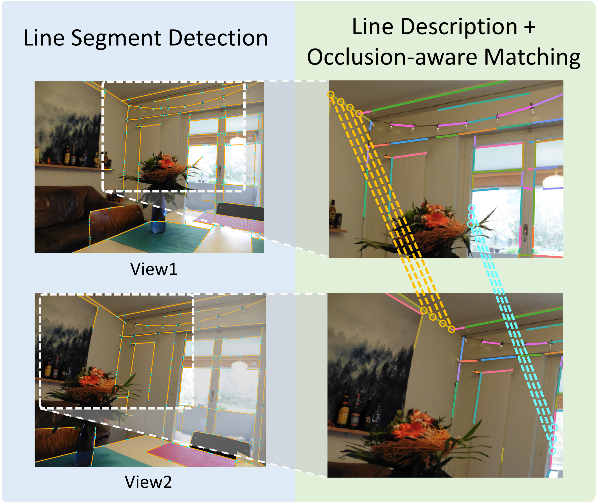
Feature points are at the core of many computer vision tasks such as Structure-from-Motion (SfM) [14, 47], Simultaneous Localization and Mapping (SLAM) [37], large-scale visual localization [44, 50] and 3D reconstruction [9], due to their compact and robust representation. Yet, the world is composed of higher-level geometric structures which are semantically more meaningful than points. Among these structures, lines can offer many benefits compared to points. Lines are widespread and frequent in the world, especially in man-made environments, and are still present in poorly textured areas. In contrast to points, they have a natural orientation, and a collection of lines provide strong geometric clues about the structure of a scene [61, 53, 16]. As such, lines represent good features for 3D geometric tasks.

Previous methods to detect line segments in images often relied on image gradient information and handcrafted filters [57, 1]. Recently, deep learning has also enabled robust and real-time line detection [19]. Most learned line detectors are however tackling a closely related task: wireframe parsing, which aims at inferring the structured layout of a scene based on line segments and their connectivity [18, 67, 63, 68]. These structures provide strong geometric cues, in particular for man-made environments. Yet, these methods have not been optimized for repeatability across images, a vital feature for multi-view tasks, and their training requires ground truth lines that are cumbersome to manually label [18].

The traditional way to match geometric structures across images is to use feature descriptors. Yet, line descriptors face several challenges: line segments can be partially occluded, their endpoints may not be well localized, the scale of the area to describe around each line fluctuates a lot, and it can be severely deformed under perspective and distortion changes [46]. Early line descriptors focused on extracting a support region around each line and on computing gradient statistics on it [60, 65]. More recently, motivated by the success of learned point descriptors [7, 9, 42], a few deep line descriptors have been proposed [25, 55, 24]. However, they are not designed to handle line occlusion and remain sensitive to poorly localized endpoints.

In this work, we propose to jointly learn the detection and description of line segments. To this end, we introduce a self-supervised network, inspired by LCNN [67] and SuperPoint [7], that can be trained on any image dataset without any labels. Pretrained on a synthetic dataset, our method is then generalized to real images. Our line detection aims at maximizing the line repeatability and at being as accurate as possible to allow its use in geometric estimation tasks. The learned descriptor is designed to be robust to occlusions, while remaining as discriminative as the current learned point descriptors. To achieve that, we introduce a novel line matching based on dynamic programming and inspired by sequence alignment in genetics [38] and classical stereo matching [8]. Thus, our self-supervised occlusion-aware line description and detection (SOLD²) offers a generic pipeline that aims at bridging the gap with the recent learned feature point methods. Overall, our contributions can be summarized as follows:

• We propose the first deep network for joint line segment detection and description.

• We show how to self-supervise our network for line detection, allowing training on any dataset of real images.

• Our line matching procedure is robust to occlusion and achieves state-of-the-art results on image matching tasks.

2 Related work

Figure 2: Training pipeline overview. Left: Our detector network is first trained on a synthetic dataset with known ground truth. Middle: A pseudo ground truth of line segments is then generated on real images through homography adaptation. Right: Finally, the full model with descriptors is trained on real images using the pseudo ground truth.

Line detection. Gradient-based line segment detection methods such as LSD [57] and EDLines [1] offer a high runtime efficiency, but are not very repeatable under viewpoint and appearance changes. Deep learning is notoriously good at tackling these issues, but learned line detectors have emerged only recently, with the introduction of the wireframe parsing [18, 63, 62, 2]. Wireframes are collections of line segments connected by their two endpoints usually labeled by humans [18]. Wireframes can be parameterized by the line junctions associated with a line verification module [18, 67], by an attraction field map (AFM) [62, 63], by a connected graph [66], by a root point and two displacements for the endpoints [19] and can benefit from a deep Hough transform prior [17, 30]. Although these methods can extract qualitatively good line segments from images, they have not been trained to produce repeatable lines under viewpoint changes and can still miss some important line landmarks for localization. We take inspiration from them but aim at detecting generic line segments generalizing to most scenes.

Line description. While early line descriptors are based on simple color histograms [4], most handcrafted descriptors leverage the image gradient [59, 60]. The most common approach is thus to extract a line support region around each line and to summarize gradient information in subregions [59, 60, 15, 65, 56]. Due to its good performance and efficiency, the Line Band Descriptor (LBD) is the most famous of them, but it still suffers from large viewpoint and appearance changes. It is only recently that line description has been tackled with deep learning. One approach is to extract a patch around the line and to compute a low dimensional embedding optimized through a triplet loss, as in DLD [25] and WLD [24]. On the other hand, a line descriptor can be considered as a collection of point descriptors, following the idea of Liu et al. [31]. The Learned Line Descriptor (LLD) [55] thus samples and describes multiple points along each line, and is conceptually the closest previous approach to our method. Designed to be fast and to be used for SLAM, it is however not invariant to rotations and its performance quickly degrades for large viewpoint changes.

Joint detection and description of learned features. Jointly learned point detectors and descriptors [45, 7, 42, 34] propose to share computation between the keypoint detection and description to get fast inference and better feature representations from multi-task learning. The describe-then-detect trend first computes a dense descriptor map and then extracts the keypoints location from it [9, 34, 64, 54]. Supervision is provided by either pixel-wise correspondences from SfM [9, 34], or from image level correspondences only [64]. HF-Net [43] unifies keypoint detection, local and global description through a multi-task distillation with multiple teacher networks. Towards the fully unsupervised spectrum, recent methods tightly couple the detector and descriptor learning to output repeatable and reliable points [5, 42, 52]. On the other hand, Superpoint [7] first learned the concept of interest points by pretraining a corner detector on a synthetic dataset and later transferring it to real world images. We adopt here a similar approach extended to line segments.

Line matching. Beyond simply comparing descriptor similarities, several works tried to leverage higher-level structural cues to guide line matching [27]. One approach considers the neighboring lines/points and finds similar patterns across images, for instance through local clusters of lines [58], intersections between lines [22] or line-junction-line structures [29, 28]. However, these methods cannot match isolated lines. Another direction is to find coplanar sets of lines and points and to leverage line-point invariants as well as simple point matching to achieve line matching [32, 10, 11, 41]. Finally, a last approach consists in matching points sampled along a line, using for example intensity information and epipolar geometry [46] or simply point descriptors [55]. Our work follows this direction but offers a flexible matching of the points along the line, which handles occlusions.

3 Method

We propose a unified network to perform line segment detection and description, allowing to match lines across different images. We achieve self-supervision in two steps. Our detector is first pretrained on a synthetic dataset with known ground truth. The full detector and descriptor can then be trained by generating pseudo ground truth line segments on real images using the pretrained model. We provide an overview of our training pipeline in Figure 2 and detail its parts in the following sections.

3.1 Problem formulation

Line segments can be parametrized in many ways: with two endpoints; with a middle point, a direction and a length; with a middle point and offsets for the endpoints; with an attraction field, etc. In this work, we chose the line representation with two endpoints for its simplicity and compatibility with our self-supervision process discussed in Section 3.4. For an image $I$ with spatial resolution $h\times w$, we thus consider in the following; the set of all junctions $P=\{p_{n}\}_{n=1}^{N}$ and line segments $L=\{l_{m}\}_{m=1}^{M}$ of $I$. A line segment $l_{m}$ is defined by a pair of endpoints $(e_{m}^{1},e_{m}^{2})\in P^{2}$.

3.2 Junction and line heatmap inference

Our network takes grayscale images as input, processes them through a shared backbone encoder that is later divided into three different outputs. A junction map $\mathbf{J}$ predicts the probability of each pixel to be a line endpoint, a line heatmap $\mathbf{H}$ provides the probability of a pixel to be on a line, and a descriptor map $\mathbf{D}$ yields a pixel-wise local descriptor. We focus here on the optimization of the first two branches, while the following sections describe their combination to retrieve and match the line segments of an image.

We adopt a similar approach to SuperPoint’s keypoint decoder [7] for the junction branch, where the output is a coarse $\frac{h}{8}\times\frac{w}{8}\times 65$ feature map $\mathbf{J^{c}}$. Each 65-dimensional vector corresponds to an $8\times 8$ patch plus an extra “no junction” dustbin. We define the ground truth junctions $\mathbf{y}\in\{1,...,65\}^{\frac{h}{8}\times\frac{w}{8}}$ indicating the index of the true junction position in each patch. A junction is randomly selected when several ground truth junctions land in the same patch and a value of $65$ means that there is no junction. The junction loss is then a cross-entropy loss between $\mathbf{J^{c}}$ and $\mathbf{y}$:

$$\mathcal{L}_{junc}=\frac{64}{h\times w}\sum_{i,j=1}^{\frac{h}{8},\frac{w}{8}}-\log\left(\frac{\exp(J^{c}_{ijy_{ij}})}{\sum_{k=1}^{65}\exp(J^{c}_{ijk})}\right)$$ (1)

At inference time, we perform a softmax on the channel dimension and discard the 65th dimension, before resizing the junction map to get the final $h\times w$ grid.

The second branch outputs a line heatmap $\mathbf{H}$ at the image resolution $h\times w$. Given a binary ground truth $\mathbf{H^{GT}}$ with a value of 1 for pixels on lines and 0 otherwise, the line heatmap is optimized via a binary cross-entropy loss:

$$\mathcal{L}_{line}=\frac{1}{h\times w}\sum_{i,j=1}^{h,w}-H^{GT}_{ij}\log(H_{ij})$$ (2)

3.3 Line detection module

After inferring the junction map $\mathbf{J}$ and line heatmap $\mathbf{H}$, we threshold $\mathbf{J}$ to keep the maximal detections and apply a non-maximum suppression (NMS) to extract the segment junctions $\hat{P}$. The line segment candidates set $\hat{L}_{cand}$ is composed of every pair of junctions in $\hat{P}$. Extracting the final line segment predictions $\hat{L}$ based on $\mathbf{H}$ and $\hat{L}_{cand}$ is non-trivial as the activations along a segment defined by two endpoints may vary a lot across different candidates. Our approach can be broken down into four parts: (1) regular sampling between endpoints, (2) adaptive local-maximum search, (3) average score, and (4) inlier ratio.

Regular sampling between endpoints: Instead of fetching all the rasterized pixels between the two endpoints [68], we sample $N_{s}$ uniformly spaced points (including the two endpoints) along the line segment.

Adaptive local-maximum search: Using bilinear interpolation to fetch the heatmap values at the extracted points $q_{k}$ may discard some candidates due to the misalignment between the endpoints and the heatmap, especially for long lines. To alleviate that, we search for the local maximal heatmap activation $h_{k}$ around each sampled location $q_{k}$ within a radius $r$ proportional to the length of the line.

Average score: The average score is defined as the mean of all the sampled heatmap values: $y_{avg}=\frac{1}{N_{s}}\sum_{k=1}^{N_{s}}h_{k}$. Given a threshold $\xi_{avg}$, valid line segment candidates should satisfy $y_{avg}\geq\xi_{avg}$.

Inlier ratio: Only relying on the average score may keep segments with a few high activations but with holes along the line. To remove these spurious detections, we also consider an inlier ratio $y_{inlier}=\frac{1}{N_{s}}\lvert\{h_{k}|h_{k}\geq\xi_{avg},h_{k}\in H\}\rvert$. Given an inlier ratio threshold $\xi_{inlier}$, we only keep candidates satisfying $y_{inlier}\geq\xi_{inlier}$.

3.4 Self-supervised learning pipeline

Inspired by the success of DeTone et al. [7], we extend their homography adaptation to the case of line segments. Let $f_{junc}$ and $f_{heat}$ represent the forward pass of our network to compute the junction map and the line heatmap. We start by aggregating the junction and heatmap predictions as in SuperPoint using a set of $N_{h}$ homographies $(\mathcal{H}_{i})_{i=1}^{N_{h}}$:

$$\mathbf{\hat{J}}(I;f_{junc}) =\frac{1}{N_{h}}\sum_{i=1}^{N_{h}}\mathcal{H}^{-1}_{i}\big{(}f_{junc}(\mathcal{H}_{i}(I))\big{)}$$ (3)

$$\mathbf{\hat{H}}(I;f_{heat}) =\frac{1}{N_{h}}\sum_{i=1}^{N_{h}}\mathcal{H}^{-1}_{i}\big{(}f_{heat}(\mathcal{H}_{i}(I))\big{)}$$ (4)

We then apply the line detection module to the aggregated maps $\mathbf{\hat{J}}$ and $\mathbf{\hat{H}}$ to obtain the predicted line segments $\hat{L}$, which are then used as ground truth for the next training round. Figure 2 provides an overview of the pipeline. Similar to Superpoint, this process can be iteratively applied to improve the label quality. However, we found that a single round of adaptation already provides sufficiently good labels.

3.5 Line description

Describing lines in images is a problem inherently more difficult than describing feature points. A line can be partially occluded, its endpoints are not always repeatable across views, and the appearance of a line can significantly differ under viewpoint changes. To tackle these challenges, we depart from the classical description of a patch centered on the line [25, 24], that is not robust to occlusions and endpoints shortening. Motivated by the success of learned point descriptors, we formulate our line descriptor as a sequence of point descriptors sampled along the line. Given a good coverage of the points along the line, even if part of the line is occluded, the points on the non-occluded part will store enough line details and can still be matched.

The descriptor head of our network outputs a descriptor map $\mathbf{D}\in\mathbb{R}^{\frac{h}{4}\times\frac{w}{4}\times 128}$ and is optimized through the classical point-based triplet loss [3, 36] used in other dense descriptors [9]. Given a pair of images $I_{1}$ and $I_{2}$ and matching lines in both images, we regularly sample points along each line and extract the corresponding descriptors $(\mathbf{D_{1}^{i}})_{i=1}^{n}$ and $(\mathbf{D_{2}^{i}})_{i=1}^{n}$ from the descriptor maps, where $n$ is total number of points in an image. The triplet loss minimizes the descriptor distance of matching points and maximizes the one of non-matching points. The positive distance is defined as

$$p_{i}=||\mathbf{D_{1}^{i}}-\mathbf{D_{2}^{i}}||_{2}$$ (5)

The negative distance is computed between a point and its hardest negative example in batch:

$$n_{i}=\min\Big{(}||\mathbf{D_{1}^{i}}-\mathbf{D_{2}^{h_{2}(i)}}||_{2},\;||\mathbf{D_{1}^{h_{1}(i)}}-\mathbf{D_{2}^{i}}||_{2}\Big{)}$$ (6)

where $h_{1}(i)=\operatorname*{arg\,min}_{\scriptsize{k\in[1,n]}}||\mathbf{D_{1}^{k}}-\mathbf{D_{2}^{i}}||$ such that the points $i$ and $k$ are at a distance of at least $T$ pixels and are not part of the same line, and similarly for $h_{2}(i)$. The triplet loss with margin $M$ is then defined as

$$\mathcal{L}_{desc}=\frac{1}{n}\sum_{i=1}^{n}\max(0,M+p_{i}-n_{i})$$ (7)

3.6 Multi-task learning

Detecting and describing lines are independent tasks with different homoscedastic aleatoric uncertainties and their respective losses can have different orders of magnitude. Thus, we adopt the multi-task learning proposed by Kendall et al. [21] with a dynamic weighting of the losses, where the weights $w_{junc}$, $w_{line}$ and $w_{desc}$ are optimized during training [20, 43]. The total loss becomes:

$$\begin{split}\mathcal{L}_{total}=\ &e^{-w_{junc}}\mathcal{L}_{junc}+e^{-w_{line}}\mathcal{L}_{line}\\ &+e^{-w_{desc}}\mathcal{L}_{desc}+w_{junc}+w_{line}+w_{desc}\end{split}$$ (8)

3.7 Line matching

At inference time, two line segments are compared based on their respective collection of point descriptors sampled along each line. However, some of the points might be occluded or, due to perspective changes, the length of a line can vary and the sampled points may be misaligned. The ordering of the points matched along the line should nevertheless be constant, i.e. the line descriptor is an ordered sequence of descriptors, not just a set. To solve this sequence assignment problem, we take inspiration from nucleotide alignment in bioinformatics [38] and pixel alignment along scanlines in stereo vision [8]. We thus propose to find the optimal point assignment through the dynamic programming algorithm originally introduced by Needleman and Wunsch [38].

When matching two sequences of points, each point can be either matched to another one or skipped. The score attributed to a match of two points depends on the similarity of their descriptors (i.e. their dot product), so that a higher similarity gives a higher score. Skipping a point is penalized by a $gap$ score, which has to be adjusted so that it is preferable to match points with high similarity but to skip the ones with low similarity. The total score of a line match is then the sum of all skip and match operations of the line points. The Needleman-Wunsch (NW) algorithm returns the optimal matching sequence maximizing this total score. This is achieved with dynamic programming by filling a matrix of scores row by row, as depicted in Figure 3. Given a sequence of $m$ points along a line $l$, $m^{\prime}$ points along $l^{\prime}$, and the associated descriptors $\mathbf{D}$ and $\mathbf{D^{\prime}}$, this score matrix $\mathbf{S}$ is an $(m+1)\times(m^{\prime}+1)$ grid where $\mathbf{S}(i,j)$ contains the optimal score for matching the first $i$ points of $l$ with the first $j$ points of $l^{\prime}$. The grid is initialized by the $gap$ score in the first row and column, and is sequentially filled row by row, using the scores stored in the left, top and top-left cells:

$$\begin{split}\mathbf{S}(i,j)=\max\big{(}&\mathbf{S}(i-1,j)+gap,\mathbf{S}(i,j-1)+gap,\\ &\mathbf{S}(i-1,j-1)+\mathbf{D^{i}}^{T}\mathbf{D^{\prime j}}\big{)}\end{split}$$ (9)

Figure 3: Computation of a line match score. The optimal path selected by the Needleman-Wunsch algorithm is shown in green for matches and blue for skipping a point, using here a $gap$ score of zero.

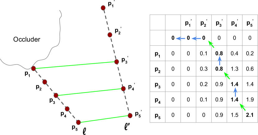
Once the matrix is filled, we select the highest score in the grid and use it as a match score for the candidate pair of lines. Each line of the first image is then matched to the line in the second image with the maximum match score.

3.8 Implementation details

Network implementation. To have a fair comparison with most wireframe parsing methods [67, 63, 30], we use the same stacked hourglass network [39] for our backbone. The three branches of our network are then series of convolutions, ReLU activations and upsampling blocks via subpixel shuffles [51]. Please refer to the supplementary material for more details about the architecture. The network is optimized with the Adam solver [23] with a learning rate of $0.0005$.

Line parameters. We use a junction threshold of $\frac{1}{65}$, a heatmap threshold $\xi_{avg}=0.25$, an inlier threshold $\xi_{inlier}=0.75$, we extract $N_{s}=64$ samples along each line to compute the heatmap and inlier scores, and we use $N_{h}=100$ homographies for the homography adaptation.

Matching details. The line descriptor is computed by regularly sampling up to 5 points along each line segment, but keeping a minimum distance of 8 pixels between each point. Since the ordering of the points might be reversed from one image to the other, we run the matching twice with one point-set flipped. A $gap$ score of $0.1$ empirically yields the best results during the NW matching. To speed up the line matching, we pre-filter the set of line candidates with a simple heuristic. Given the descriptor of the 5 points sampled on a line of $I_{1}$ to be matched, we compute the similarity with their nearest neighbor in each line of $I_{2}$, and average these scores for each line. This yields a rough estimate of the line match score, and we keep the top 10 best lines as candidates for the NW matching. Finally, we retain at matching time only the pairs that are mutually matched.

Training dataset. We use the same synthetic dataset as in SuperPoint [7], labelling the corners of the geometrical shapes as junctions and edges as line segments. For the training with real images, we use the Wireframe dataset [18], allowing a fair comparison with the current state of the art also trained on these images. We follow the split policy in LCNN [67]: $5,000$ images for training and $462$ images for testing. We however only use the images and ignore the ground truth lines provided by the dataset.

4 Experiments

	Wireframe Dataset [18]						YorkUrban Dataset [6]
	$\operatorname{d_{s}}$		$\operatorname{d_{orth}}$		time$\downarrow$	# lines / image	$\operatorname{d_{s}}$		$\operatorname{d_{orth}}$		time$\downarrow$	# lines / image
	$\mathrm{Rep\text{-}}5$ $\uparrow$	$\mathrm{LE\text{-}5}$ $\downarrow$	$\mathrm{Rep\text{-}5}$ $\uparrow$	$\mathrm{LE\text{-}5}$ $\downarrow$			$\mathrm{Rep\text{-}5}$ $\uparrow$	$\mathrm{LE\text{-}5}$ $\downarrow$	$\mathrm{Rep\text{-}5}$ $\uparrow$	$\mathrm{LE\text{-}5}$ $\downarrow$
LCNN [67] @0.98	0.434	2.589	0.570	1.725	0.120	76	0.318	2.662	0.449	1.784	0.206	103
HAWP [63] @0.97	0.451	2.625	0.537	1.738	0.035	47	0.295	2.566	0.368	1.757	0.045	59
DeepHough [30] @0.9	0.419	2.576	0.618	1.720	0.289	135	0.315	2.695	0.535	1.751	0.519	206
TP-LSD [19] HG	0.358	3.220	0.647	2.212	0.038	72	0.233	3.357	0.524	2.395	0.038	113
TP-LSD [19] TP512	0.563	2.467	0.746	1.450	0.097	81	0.433	2.612	0.633	1.555	0.099	125
LSD [57]	0.358	2.079	0.707	0.825	0.026	228	0.357	2.116	0.704	0.876	0.031	359
Ours w/ CS	0.557	1.995	0.801	1.119	0.042	116	0.528	1.902	0.787	1.107	0.064	222
Ours	0.616	2.019	0.914	0.816	0.074	447	0.582	1.932	0.913	0.713	0.093	1085

Table 1: Line detection evaluation on the Wireframe [18] and YorkUrban [6] datasets. We compare repeatability and localization error for an error threshold of 5 pixels in structural and orthogonal distances. Our approach provides the most repeatable and accurate line detections compared to the other baselines.

4.1 Line segment detection evaluation

To evaluate our line segment detection, we use the test split of the Wireframe dataset [18] and the YorkUrban dataset [6], which contains 102 outdoor images. For both datasets, we generate a fixed set of random homographies and warp each image to get a pair of matching images.

Line segment distance metrics. A line distance metric needs to be defined to evaluate the accuracy of a line detection. We use the two following metrics:

Structural distance ($\operatorname{\mathbf{d_{s}}}$): The structural distance of two line segments $l_{1}$ and $l_{2}$ is defined as:

$$\begin{split}\operatorname{d_{s}}(l_{1},l_{2})=\min(&\lVert e_{1}^{1}-e_{2}^{1}\rVert_{2}+\lVert e_{1}^{2}-e_{2}^{2}\rVert_{2},\\ &\lVert e_{1}^{1}-e_{2}^{2}\rVert_{2}+\lVert e_{1}^{2}-e_{2}^{1}\rVert_{2})\end{split}$$ (10)

where $(e_{1}^{1},e_{1}^{2})$ and $(e_{2}^{1},e_{2}^{2})$ are the endpoints of $l_{1}$ and $l_{2}$ respectively. Contrary to the formulation of recent wireframe parsing works [67, 63], we do not use square norms to make it directly interpretable in terms of endpoints distance.

Orthogonal distance ($\operatorname{\mathbf{d_{orth}}}$): The orthogonal distance of two line segments $l_{1}$ and $l_{2}$ is defined as the average of two asymmetrical distances $d_{a}$:

$$\operatorname{d_{a}}(l_{i},l_{j})=\lVert e_{j}^{1}-p_{l_{i}}(e_{j}^{1})\rVert_{2}+\lVert e_{j}^{2}-p_{l_{i}}(e_{j}^{2})\rVert_{2}$$ (11)

$$\operatorname{d_{orth}}(l_{1},l_{2})=\frac{\operatorname{d_{a}}(l_{1},l_{2})+\operatorname{d_{a}}(l_{2},l_{1})}{2}$$ (12)

where $p_{l_{j}}(.)$ denotes the orthogonal projection on line $l_{j}$. When searching the nearest line segment with this distance, we ignore the line segments with an overlap below $0.5$. This definition allows line segments corresponding to the same 3D line but with different line lengths to be considered as close, which can be useful in localization tasks [35].

Line segment detection metrics. Since the main objective of our line segment detection method is to extract repeatable and reliable line segments from images, evaluating it on the manually labeled lines of the wireframe dataset [18] is not suitable. We thus instead adapt the detector metrics proposed for SuperPoint [7] to line segments using pairs of images.

Repeatability: The repeatability measures how often a line can be re-detected in different views. It is the average percentage of lines in the first image that have a matching line when reprojected in the second image. Two lines are considered to be matched when their distance is lower than a threshold $\epsilon$. This metric is computed symmetrically across the two images and averaged.

Localization error: The localization error with tolerance $\epsilon$ is the average line distance between a line and its re-detection in the second image, only considering the matched lines.

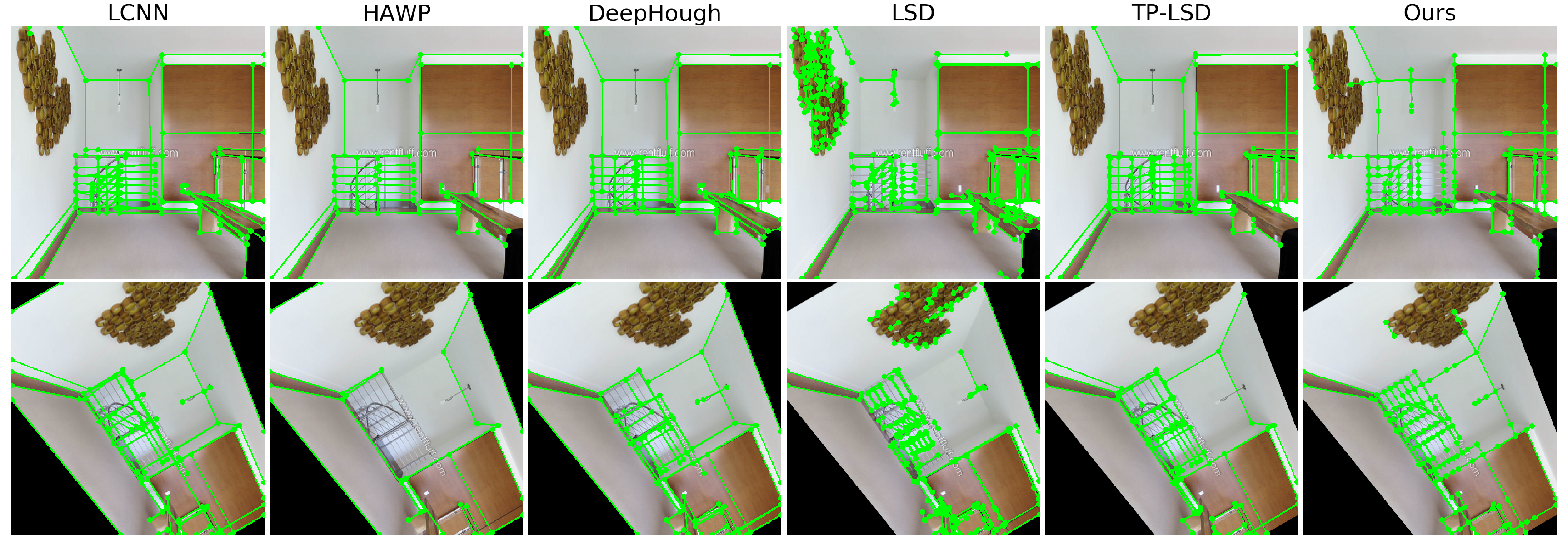
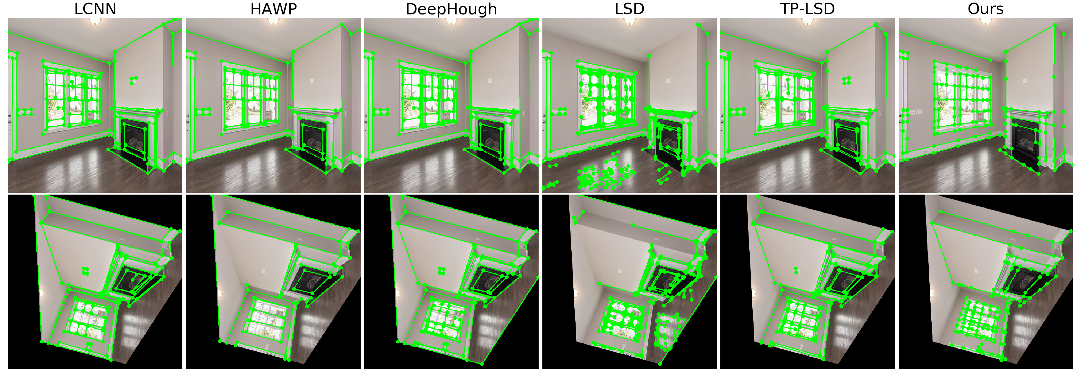
Evaluation on the Wireframe and YorkUrban datasets. We compare in Table 4 our line segment detection method with 5 baselines including the handcrafted Line Segment Detection (LSD) [57], wireframe parsing methods such as LCNN [67], HAWP [63], TP-LSD [19], and Deep Hough-transform Line Priors (DeepHough) [30]. LSD is used with a minimum segment length of 15 pixels. For LCNN, HAWP, and DeepHough, we chose thresholds (0.98, 0.97, and 0.9 respectively) on the line scores to maximize their performances. We show two TP-LSD variants: HG using the same backbone [39] as the other wireframe parsing baselines and our method, and TP512 that uses a ResNet34 [13] backbone.

Overall, our method achieves the best performance in terms of repeatability and localization error on both datasets. We also include our method with candidate selection (CS), which removes the segments having other junctions between the two endpoints to avoid overlapping segments in the predictions $\hat{L}$. Without overlapping segments, the performance slightly decreases but we get fewer segments and faster inference speed. The candidate selection is also used in our descriptor evaluation section and is referred as line NMS.

4.2 Line segment description evaluation

Line descriptor metrics. Our line descriptor is evaluated on several matching metrics, both on hand-labeled line segments and on detected line segments (LSD or our predicted lines). When using ground truth lines, there is an exact one-to-one line correspondence. For predicted lines, ground truth matches are computed with a threshold $\epsilon$ similarly as for the detector metrics. When depth is available, the lines are projected to 3D and directly compared in 3D space. Only lines with a valid reprojection in the other image are considered.

Accuracy: Percentage of correctly matched lines given a set of ground truth line matches.

Receiver operating characteristic (ROC) curve: Given a set of matching lines, we compute the SIFT [33] descriptor of each endpoint, average the SIFT distances between each pair of lines, and use the second nearest neighboring line as negative match. The ROC curve is then the true positive rate (TPR) plotted against the false positive rate (FPR). The curve is obtained by varying the descriptor similarity threshold defining a positive match.

Precision: Ratio of true positive matches over the total number of predicted matches.

Recall: Ratio of true positive matches over the total number of ground truth matches.

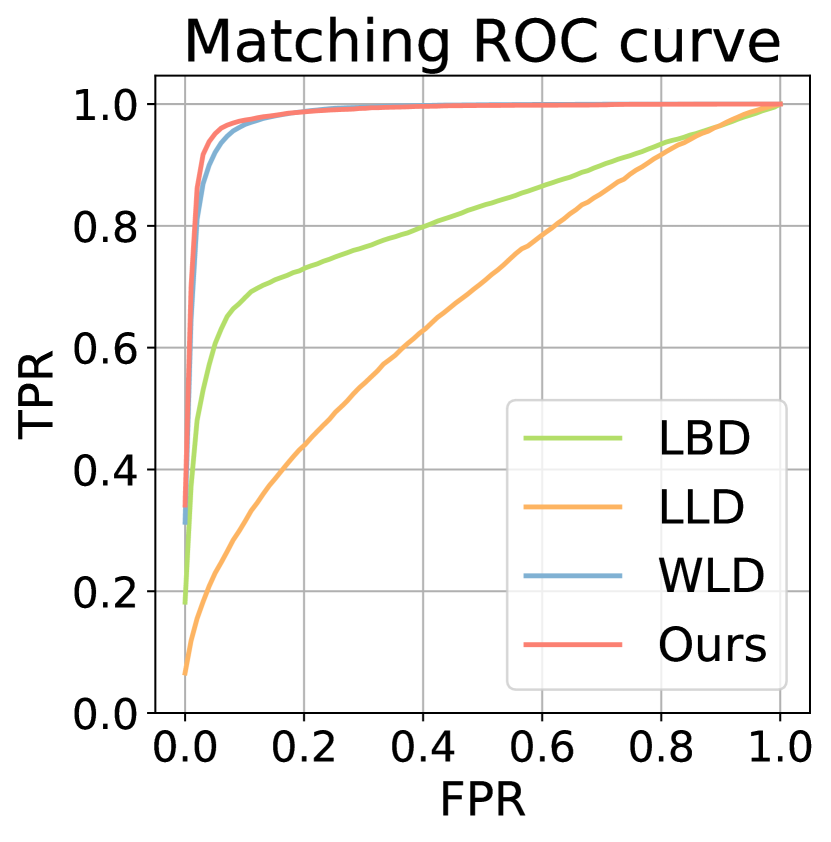
Descriptor evaluation on ground truth lines. Our first experiment aims at evaluating our approach on a perfect set of lines with a one-to-one matching. We thus use the Wireframe test set with its ground truth lines. We compare our line matcher against 3 competing baselines: the handcrafted Line Band Descriptor (LBD) [65], the Learnable Line Descriptor (LLD) [55] and the Wavelet Line Descriptor (WLD) [24], an improved version of the Deep Line Descriptor (DLD) [25]. The results are shown in Figure 4.

Since LLD was trained on consecutive video frames with nearly no rotation between the images, it is not rotation invariant, hence its poor performance on the rotated images of our dataset. WLD showed that they were able to surpass the handcrafted LBD, and our descriptor gets a slight improvement over WLD by $5\%$.

Method	Accuracy$\uparrow$
LBD [65]	0.610
LLD [55]	0.265
WLD [24]	0.933
SOLD2 (Ours)	0.978

Figure 4: Descriptor evaluation on the Wireframe [18] dataset with ground truth lines. Matching the exact same lines yields a very high score for WLD and our method.

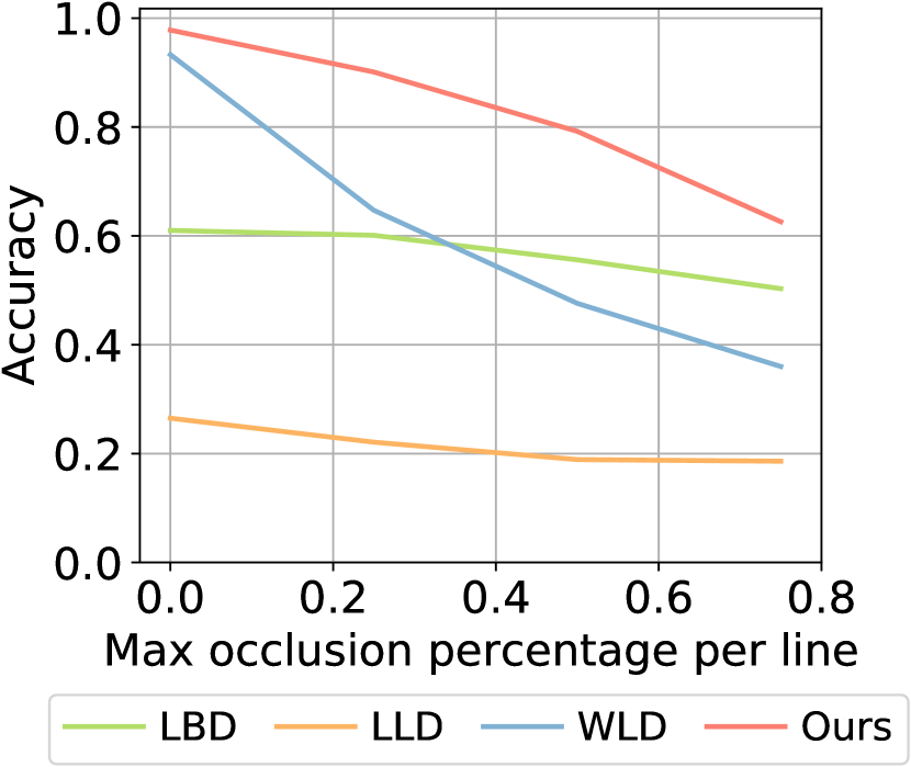
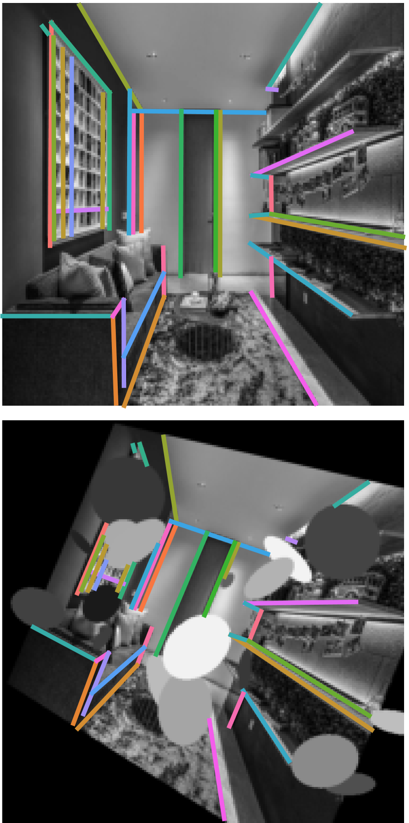
Robustness to occlusion experiment. In real-world applications, the detected lines across multiple views are rarely exactly the same, and some may be partially occluded or with different endpoints. To evaluate the robustness of our descriptor to these challenges, we modify the Wireframe test set to include artificial occluders. More precisely, we overlay ellipses with random parameters and synthetic textures on the warped image of each pair, until at most $s\%$ of the lines are covered. We also shorten the line segments accordingly, so that each line stops at the occluders boundary. We compare line matches for various values of $s$ and get the results presented in Figure 5.

While all methods show a decrease in performance with a larger occlusion, SOLD² outperforms the other baselines by a large margin for all degrees of occlusion. Note the significant drop for the learned baseline WLD, which operates on line patches and is thus severely affected by occlusions. This experiment thus validates the robustness of our method to occlusion and unstable line endpoints.

Figure 5: Robustness to occlusion. Left: When evaluated on the Wireframe dataset with ground truth lines and random occluders, our method shows a higher robustness to occlusion compared to other methods. Right: Example of matches in the presence of occluders.

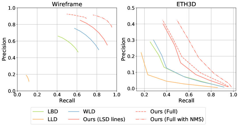
Descriptor evaluation on predicted lines. To assess the performance of our proposed line description and matching, we also compute the matching metrics on predicted line segments instead of using hand-labeled lines. We perform two sets of experiments, on the Wireframe test set and on the ETH3D [49] images which offer real world camera motions and can contain more challenging viewpoint changes than homographic warps. For the latter, images are downsampled by a factor of 8 and we select all pairs of images that share at least 500 covisible 3D points in the provided 3D models. In both experiments, we run the LSD detector and compute all the line descriptor methods on them and also compare it with our full line prediction and description. Table 4.2 and Figure 6 evaluate the precision and recall of all methods.

Whether it is on synthetically warped images, or with real camera changes, SOLD² outperforms all the descriptor baselines both in terms of matching precision and recall when compared on LSD lines. Using our own lines also improves the metrics, but the best performance is achieved when we apply a line NMS to remove overlapping segments. Having no overlap makes it indeed easier for the descriptor to discriminate the closest matching line.

		Wireframe [18]		ETH3D [49]
Lines	Desc	Precision$\uparrow$	Recall$\uparrow$	Precision$\uparrow$	Recall$\uparrow$
LSD [57]	LBD [65]	0.496	0.597	0.132	0.376
	LLD [55]	0.123	0.116	0.085	0.230
	WLD [24]	0.528	0.804	0.127	0.398
	SOLD2 (Ours)	0.591	0.889	0.159	0.525
Ours	SOLD2 (Ours)	0.882	0.688	0.196	0.538
Ours w/ NMS	SOLD2 (Ours)	0.777	0.949	0.190	0.688

Table 2: Matching precision and recall using LSD [57] and our lines. We use a threshold of 5 pixels in structural distance for the Wireframe [18] images and of 5cm for the ETH3D images to define the ground truth matches.

Figure 6: Precision-Recall curves on predicted lines. Our descriptor outperforms the other baselines when compared on LSD lines and the best performance is achieved for our full approach with our lines and descriptors.

4.3 Ablation study

To validate the design choices of our approach, we perform an ablation study on the descriptor. SIFT endpoints computes a SIFT descriptor [33] for both endpoints using the line direction as keypoint orientation, and averages the endpoints descriptor distance of each line candidate pair to get the line match scores. Average descriptor computes a line descriptor by averaging the descriptors of all the points sampled along each line. NN average computes the descriptor similarity of each line point with its nearest neighbor in the other line and averages all the similarities to get a line match score. D2-Net sampling and ASLFeat sampling refer to our proposed matching method where the points are sampled along the lines according to the saliency score introduced in D2-Net [9] and ASLFeat [34], respectively. Finally, we test our method with various numbers of points sampled along each line. Table LABEL:tab:ablation_study compares the accuracy of all these methods on the Wireframe dataset with ground truth lines both with and without occluders.

	$\operatorname{d_{s}}$		$\operatorname{d_{orth}}$
	$\mathrm{Rep\text{-}5}$ $\uparrow$	$\mathrm{LE\text{-}5}$ $\downarrow$	$\mathrm{Rep\text{-}5}$ $\uparrow$	$\mathrm{LE\text{-}5}$ $\downarrow$
LCNN [67]	0.336	2.777	0.637	1.878
HAWP [63]	0.451	2.625	0.537	1.738
DeepHough [30]	0.370	2.676	0.652	1.777
TP-LSD [19]	0.563	2.467	0.746	1.450
LSD [57]	0.358	2.079	0.707	0.825
Ours (mean)	0.577	1.955	0.891	0.804
Std deviation	0.020	0.070	0.0055	0.023

Figure 9: Statistical significance of the evaluation. We report the average value $\mu$ and standard deviation $\sigma$ of 5 different training runs of our method on the Wireframe dataset [18]. Left: repeatability and localization error of the detector. Right: matching precision-recall curve with confidence interval $[\mu-\sigma,\mu+\sigma]$.

Appendix G ETH3D dataset preprocessing

The ETH3D dataset [49] is composed of 13 scenes taken in indoor as well as outdoor environments. Each image comes with the corresponding camera intrinsics and depth map, and a 3D model of each scene built with Colmap [48] is provided as well. We use the undistorted image downsampled by a factor of 8 to run the line detection and description. We then use the depth maps and camera intrinsics to reproject the lines in 3D and compute the descriptor metrics in 3D space. While the depth maps have been obtained from a high-precision laser scanner, they contain some holes, in particular close to depth discontinuities. Since these discontinuities are actually where lines are often located, we inpaint the depth in all of the invalid areas at up to 10 pixels from a valid depth pixel. We used NLSPN [40], the current state of the art in deep depth inpainting guided with RGB images.

LSD [57]      + LBD [65]
LSD [57]      + LLD [55]
LSD [57]      + WLD [24]
Ours

Figure 10: Qualitative results of line segment matching. We display line segment matches on the ETH3D dataset [49] with correct matches, wrong matches and unmatched lines. Only lines shared between the two views are shown. Our full pipeline is compared to three line descriptor baselines computed on LSD lines [57]: LBD [65], LLD [55] and WLD [24].

View2                         View1
View2                         View1
View2                         View1
View2                         View1

Figure 11: Qualitative results of line segment detections. We show examples of line detections on the Wireframe dataset [18] for the following methods: LCNN [67], HAWP [63], DeepHough [30], LSD [57], TP-LSD [19] and ours.

Appendix H Homography estimation experiment

To validate the real-world applications of our method, we used the line segment detections and descriptors to match segments across pairs of images of the Wireframe dataset related by a homography [18] and estimate the homography with RANSAC [12]. We sample minimal sets of 4 lines to fit a homography and run up to $1,000,000$ iterations with the LORANSAC [26] implementation of Sattler et al.. The reprojection error is computed with the orthogonal line distance. We compute the accuracy of the homography estimation similarly as in SuperPoint [7] by warping the four corners of the image with the estimated homography, warping them back to the initial image with the ground truth homography and computing the reprojection error of the corners. We consider the estimated homography to be correct if the average reprojection error is less than 3 pixels. The results are listed in Table H.

When compared on LSD line [57], our descriptors provide the highest accuracy among all baselines, and our full pipeline achieves a similar performance. When using our lines, we use a similar refinement of the junctions as in LSD [57]: we sample small perturbations of the endpoints by a quarter of a pixel and keep the perturbed endpoints maximizing the line average score. Similarly to feature point methods [7, 9], this experiment shows that learned features are still on par or slightly worse than handcrafted detections in terms of localization error.

We also add to the comparison the results of homography estimation for a learned feature point detector and descriptor, SuperPoint [7]. The point-based approach performs significantly worse than our method, due to the numerous textureless scenes and repeated structures present in the Wireframe dataset. We also found that SuperPoint is not robust to rotations above 45 degrees, while our line descriptor can leverage its ordered sequence of descriptors to achieve invariance with respect to any rotation.

		Homography estimation
Lines	Desc	Accuracy$\uparrow$	# inliers	Reproj. error$\downarrow$
LSD [57]	LBD [65]	0.781	80	0.791
	LLD [55]	0.201	21	0.927
	WLD [24]	0.920	116	0.868
	Ours	0.948	116	0.863
Ours	Ours	0.935	200	0.780
SuperPoint [7]		0.582	173	0.996

Table 4: Evaluation results of homography estimation. The homography between images of the Wireframe dataset [18] is estimated from line matches using RANSAC. We use a threshold of 5 pixels in orthogonal line distance to consider a match to be an inlier.

Appendix I Qualitative results of line segment detections and matches

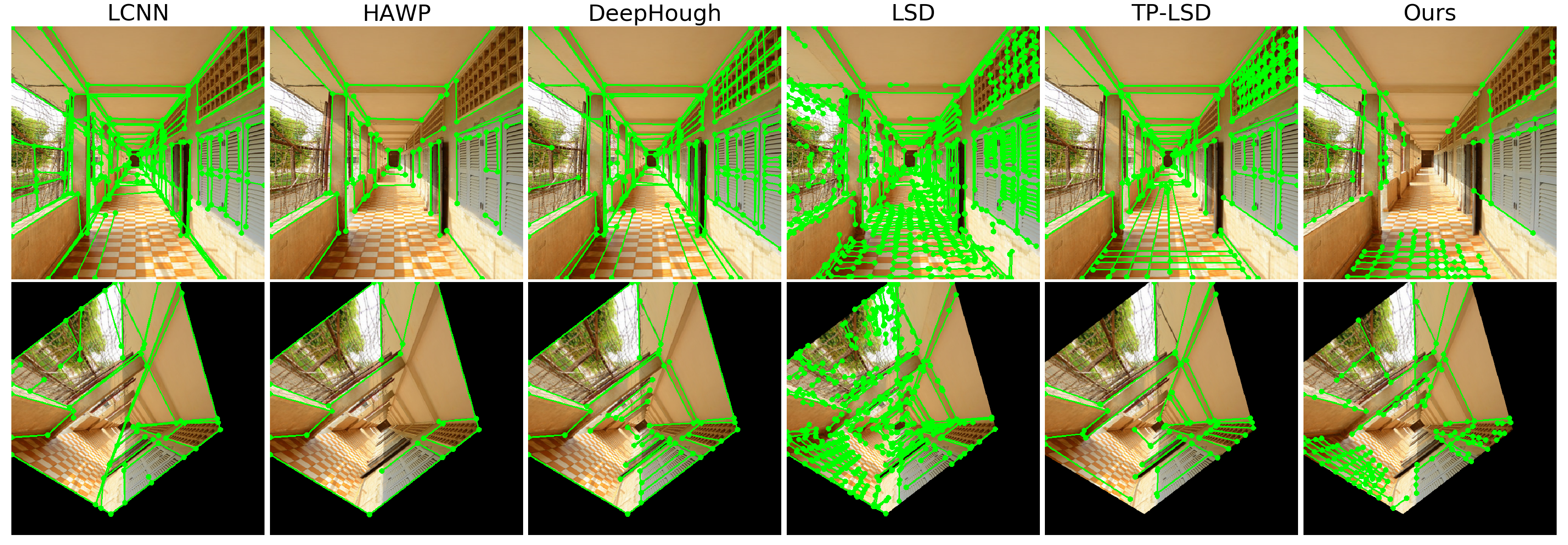
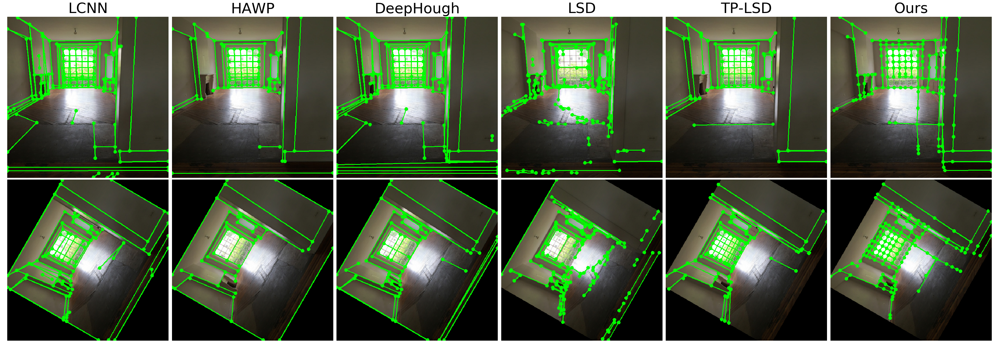
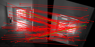
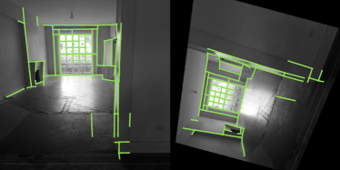
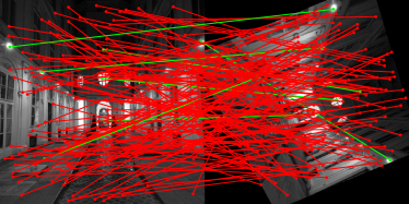
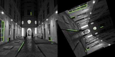
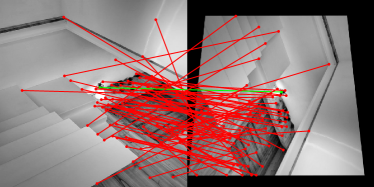
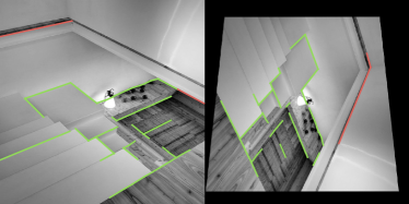
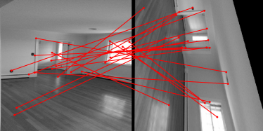
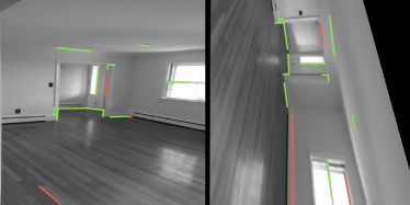
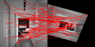
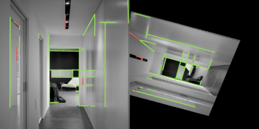
We provide some visualizations of the line segment detection results in Figure 11 and of the line matching in Figure 10. Figure 12 also offers a comparison of line matches with point matches in challenging images with low texture, and repeated structures. Our method is able to match enough lines to obtain an accurate pose estimation, while point-based methods such as SuperPoint [7] fail in such scenarios.

SuperPoint [7]	Ours

Figure 12: Benefits of lines compared to feature points. We compare our method with point matching from SuperPoint [7] on challenging images of the Wireframe dataset [18] with correct and wrong matches. We use a distance threshold of 5 pixels to determine if a match is correct, using the orthogonal line distance in the case of lines. Lines can be matched even in the presence of textureless areas, as well as repeated and symmetrical structures.

References

- [1] C. Akinlar and C. Topal. Edlines: Real-time line segment detection by edge drawing. In International Conference on Image Processing (ICIP), 2011.
- [2] Emilio J Almazan, Ron Tal, Yiming Qian, and James H Elder. Mcmlsd: A dynamic programming approach to line segment detection. In Computer Vision and Pattern Recognition (CVPR), 2017.
- [3] Vassileios Balntas, Edgar Riba, Daniel Ponsa, and Krystian Mikolajczyk. Learning local feature descriptors with triplets and shallow convolutional neural networks. In British Machine Vision Conference (BMVC), 2016.
- [4] Herbert Bay, Vittorio Ferraris, and Luc Van Gool. Wide-baseline stereo matching with line segments. In Computer Vision and Pattern Recognition (CVPR), 2005.
- [5] Peter Hviid Christiansen, Mikkel Fly Kragh, Yury Brodskiy, and Henrik Karstoft. Unsuperpoint: End-to-end unsupervised interest point detector and descriptor. arXiv, 2019.
- [6] Patrick Denis, James H Elder, and Francisco J Estrada. Efficient edge-based methods for estimating manhattan frames in urban imagery. In European Conference on Computer Vision (ECCV), 2008.
- [7] Daniel DeTone, Tomasz Malisiewicz, and Andrew Rabinovich. Superpoint: Self-supervised interest point detection and description. In Computer Vision and Pattern Recognition Workshops (CVPRW), 2018.
- [8] Romain Dieny, Jerome Thevenon, Jesus Martinez del rincon, and Jean christophe Nebel. Bioinformatics inspired algorithm for stereo correspondence. In International Conference on Computer Vision Theory and Applications (VISAPP), 2011.
- [9] Mihai Dusmanu, Ignacio Rocco, Tomas Pajdla, Marc Pollefeys, Josef Sivic, Akihiko Torii, and Torsten Sattler. D2-Net: A Trainable CNN for Joint Detection and Description of Local Features. In Computer Vision and Pattern Recognition (CVPR), 2019.
- [10] Bin Fan, Fuchao Wu, and Zhanyi Hu. Line matching leveraged by point correspondences. In Computer Vision and Pattern Recognition (CVPR), 2010.
- [11] Bin Fan, Fuchao Wu, and Zhanyi Hu. Robust line matching through line–point invariants. Pattern Recognition, 45, 2012.
- [12] Martin A. Fischler and Robert C. Bolles. Random sample consensus: A paradigm for model fitting with applications to image analysis and automated cartography. Communication of the ACM, 24(6), 1981.
- [13] Kaiming He, Xiangyu Zhang, Shaoqing Ren, and Jian Sun. Deep residual learning for image recognition. In Computer Vision and Pattern Recognition (CVPR), 2016.
- [14] Jared Heinly, Johannes Lutz Schönberger, Enrique Dunn, and Jan-Michael Frahm. Reconstructing the World* in Six Days *(As Captured by the Yahoo 100 Million Image Dataset). In Computer Vision and Pattern Recognition (CVPR), 2015.
- [15] Keisuke Hirose and Hideo Saito. Fast line description for line-based slam. In British Machine Vision Conference (BMVC), 2012.
- [16] Aleksander Holynski, David Geraghty, Jan-Michael Frahm, Chris Sweeney, and Richard Szeliski. Reducing drift in structure from motion using extended features. arXiv, 2020.
- [17] Paul VC Hough. Method and means for recognizing complex patterns, 1962. US Patent 3,069,654.
- [18] Kun Huang, Yifan Wang, Zihan Zhou, Tianjiao Ding, Shenghua Gao, and Yi Ma. Learning to parse wireframes in images of man-made environments. In Computer Vision and Pattern Recognition (CVPR), 2018.
- [19] Siyu Huang, Fangbo Qin, Pengfei Xiong, Ning Ding, Yijia He, and Xiao Liu. Tp-lsd: Tri-points based line segment detector. In European Conference on Computer Vision (ECCV), 2020.
- [20] Alex Kendall and Roberto Cipolla. Geometric loss functions for camera pose regression with deep learning. In Computer Vision and Pattern Recognition (CVPR), 2017.
- [21] Alex Kendall, Yarin Gal, and Roberto Cipolla. Multi-task learning using uncertainty to weigh losses for scene geometry and semantics. In Computer Vision and Pattern Recognition (CVPR), 2018.
- [22] Hyunwoo Kim and Sukhan Lee. A novel line matching method based on intersection context. In International Conference on Robotics and Automation (ICRA), 2010.
- [23] Diederik Kingma and Jimmy Ba. Adam: A method for stochastic optimization. International Conference on Learning Representations (ICLR), 2014.
- [24] Manuel Lange, Claudio Raisch, and Andreas Schilling. Wld: A wavelet and learning based line descriptor for line feature matching. In International Symposium on Vision, Modeling, and Visualization (VMV), 2020.
- [25] Manuel Lange, Fabian Schweinfurth, and Andreas Schilling. DLD: A Deep Learning Based Line Descriptor for Line Feature Matching. In International Conference on Intelligent Robots and Systems (IROS), 2019.
- [26] Karel Lebeda, Jiri Matas, and Ondrej Chum. Fixing the Locally Optimized RANSAC. In British Machine Vision Conference (BMVC), 2012.
- [27] Kai Li, Jian Yao, Mengsheng Lu, Yuan Heng, Teng Wu, and Yinxuan Li. Line segment matching: a benchmark. In Winter Conference on Applications of Computer Vision (WACV), 2016.
- [28] Kai Li, Jian Yao, and Xiaohu Lu. Robust line matching based on ray-point-ray structure descriptor. In Asian Conference on Computer Vision (ACCV), pages 554–569, 2014.
- [29] Kai Li, Jian Yao, Xiaohu Lu, Li Li, and Zhichao Zhang. Hierarchical line matching based on line–junction–line structure descriptor and local homography estimation. Neurocomputing, 184:207–220, 2016.
- [30] Yancong Lin, Silvia L Pintea, and Jan C van Gemert. Deep hough-transform line priors. In European Conference on Computer Vision (ECCV), 2020.
- [31] Hong-Min Liu, Zhi-Heng Wang, and Chao Deng. Extend point descriptors for line, curve and region matching. In International Conference on Machine Learning and Cybernetics (ICMLC), volume 1, pages 214 – 219, 08 2010.
- [32] Manolis I. A. Lourakis, Spyros T. Halkidis, and Stelios C. Orphanoudakis. Matching disparate views of planar surfaces using projective invariants. In British Machine Vision Conference (BMVC), 1998.
- [33] David G. Lowe. Distinctive image features from scale-invariant keypoints. International Journal of Computer Vision (IJCV), 60, 2004.
- [34] Zixin Luo, Lei Zhou, Xuyang Bai, Hongkai Chen, Jiahui Zhang, Yao Yao, Shiwei Li, Tian Fang, and Long Quan. Aslfeat: Learning local features of accurate shape and localization. Computer Vision and Pattern Recognition (CVPR), 2020.
- [35] B. Micusik and H. Wildenauer. Structure from motion with line segments under relaxed endpoint constraints. In International Conference on 3D Vision (3DV), volume 1, 2014.
- [36] Anastasiya Mishchuk, Dmytro Mishkin, Filip Radenović, and Jiri Matas. Working hard to know your neighbor’s margins:local descriptor learning loss. In Neural Information Processing Systems (NIPS), 2017.
- [37] R. Mur-Artal, J. M. M. Montiel, and J. D. Tardós. Orb-slam: A versatile and accurate monocular slam system. IEEE Transactions on Robotics, 31(5), 2015.
- [38] Saul B. Needleman and Christian D. Wunsch. A general method applicable to the search for similarities in the amino acid sequence of two proteins. Journal of Molecular Biology, 48(3):443 – 453, 1970.
- [39] Alejandro Newell, Kaiyu Yang, and Jia Deng. Stacked hourglass networks for human pose estimation. In European Conference on Computer Vision (ECCV), 2016.
- [40] Jinsun Park, Kyungdon Joo, Zhe Hu, Chi-Kuei Liu, and In So Kweon. Non-local spatial propagation network for depth completion. In Proc. of European Conference on Computer Vision (ECCV), 2020.
- [41] Srikumar Ramalingam, Michel Antunes, Dan Snow, Gim Hee Lee, and Sudeep Pillai. Line-sweep: Cross-ratio for wide-baseline matching and 3d reconstruction. In Computer Vision and Pattern Recognition (CVPR), 2015.
- [42] Jerome Revaud, Philippe Weinzaepfel, César Roberto de Souza, and Martin Humenberger. R2D2: repeatable and reliable detector and descriptor. In Neural Information Processing Systems (NeurIPS), 2019.
- [43] Paul-Edouard Sarlin, Cesar Cadena, Roland Siegwart, and Marcin Dymczyk. From coarse to fine: Robust hierarchical localization at large scale. In Computer Vision and Pattern Recognition (CVPR), 2019.
- [44] T. Sattler, A. Torii, J. Sivic, M. Pollefeys, H. Taira, M. Okutomi, and T. Pajdla. Are large-scale 3d models really necessary for accurate visual localization? In Computer Vision and Pattern Recognition (CVPR), 2017.
- [45] Torsten Sattler, Qunjie Zhou, Marc Pollefeys, and Laura Leal-Taixe. Understanding the limitations of cnn-based absolute camera pose regression. In Computer Vision and Pattern Recognition (CVPR), 2019.
- [46] Cordelia Schmid and Andrew Zisserman. Automatic line matching across views. In Computer Vision and Pattern Recognition (CVPR), 1997.
- [47] Johannes L Schonberger and Jan-Michael Frahm. Structure-from-motion revisited. In Computer Vision and Pattern Recognition (CVPR), 2016.
- [48] Johannes Lutz Schönberger and Jan-Michael Frahm. Structure-from-motion revisited. In Conference on Computer Vision and Pattern Recognition (CVPR), 2016.
- [49] Thomas Schöps, Johannes L. Schönberger, Silvano Galliani, Torsten Sattler, Konrad Schindler, Marc Pollefeys, and Andreas Geiger. A multi-view stereo benchmark with high-resolution images and multi-camera videos. In Computer Vision and Pattern Recognition (CVPR), 2017.
- [50] Johannes L. Schönberger, Marc Pollefeys, Andreas Geiger, and Torsten Sattler. Semantic visual localization. In Computer Vision and Pattern Recognition (CVPR), 2017.
- [51] Wenzhe Shi, Jose Caballero, Ferenc Huszár, Johannes Totz, Andrew P Aitken, Rob Bishop, Daniel Rueckert, and Zehan Wang. Real-time single image and video super-resolution using an efficient sub-pixel convolutional neural network. In Computer Vision and Pattern Recognition (CVPR), 2016.
- [52] Yafei Song, Ling Cai, Jia Li, Yonghong Tian, and Mingyang Li. SEKD: Self-evolving keypoint detection and description. arXiv, 2020.
- [53] Camillo J Taylor and David J Kriegman. Structure and motion from line segments in multiple images. IEEE Transactions on Pattern Analysis and Machine Intelligence (PAMI), 17(11):1021–1032, 1995.
- [54] Yurun Tian, Vassileios Balntas, Tony Ng, Axel Barroso, Yiannis Demiris, and Krystian Mikolajczyk. D2d: Keypoint extraction with describe to detect approach. arXiv, 2020.
- [55] A. Vakhitov and V. Lempitsky. Learnable line segment descriptor for visual slam. IEEE Access, 7, 2019.
- [56] Bart Verhagen, Radu Timofte, and Luc Van Gool. Scale-invariant line descriptors for wide baseline matching. In Winter Conference on Applications of Computer Vision (WACV), 2014.
- [57] Rafael Grompone Von Gioi, Jeremie Jakubowicz, Jean-Michel Morel, and Gregory Randall. Lsd: A fast line segment detector with a false detection control. IEEE Transactions on Pattern Analysis and Machine Intelligence (PAMI), 32(4):722–732, 2008.
- [58] Lu Wang, Ulrich Neumann, and Suya You. Wide-baseline image matching using line signatures. In International Conference on Computer Vision (ICCV), 2009.
- [59] Zhiheng Wang, Hong-Min Liu, and Fuchao Wu. Hld: A robust descriptor for line matching. In Conference on Computer-Aided Design and Computer Graphics, 2009.
- [60] Zhiheng Wang, Fuchao Wu, and Zhanyi Hu. Msld: A robust descriptor for line matching. Pattern Recognition, 42(5):941–953, 2009.
- [61] Juyang Weng, Thomas S. Huang, and Narendra Ahuja. Motion and structure from line correspondences; closed-form solution, uniqueness, and optimization. IEEE Transactions on Pattern Analysis and Machine Intelligence (PAMI), 14(3):318–336, 1992.
- [62] Nan Xue, Song Bai, Fudong Wang, Gui-Song Xia, Tianfu Wu, and Liangpei Zhang. Learning attraction field representation for robust line segment detection. In Computer Vision and Pattern Recognition (CVPR), 2019.
- [63] Nan Xue, Tianfu Wu, Song Bai, Fudong Wang, Gui-Song Xia, Liangpei Zhang, and Philip HS Torr. Holistically-attracted wireframe parsing. In Computer Vision and Pattern Recognition (CVPR), 2020.
- [64] Tsun-Yi Yang, Duy-Kien Nguyen, Huub Heijnen, and Vassileios Balntas. Ur2kid: Unifying retrieval, keypoint detection, and keypoint description without local correspondence supervision. arXiv, 2020.
- [65] Lilian Zhang and Reinhard Koch. An efficient and robust line segment matching approach based on lbd descriptor and pairwise geometric consistency. Journal of Visual Communication and Image Representation, 24(7), 2013.
- [66] Ziheng Zhang, Zhengxin Li, Ning Bi, Jia Zheng, Jinlei Wang, Kun Huang, Weixin Luo, Yanyu Xu, and Shenghua Gao. Ppgnet: Learning point-pair graph for line segment detection. In Computer Vision and Pattern Recognition (CVPR), 2019.
- [67] Yichao Zhou, Haozhi Qi, and Yi Ma. End-to-end wireframe parsing. In International Conference on Computer Vision (ICCV), 2019.
- [68] Yichao Zhou, Haozhi Qi, Yuexiang Zhai, Qi Sun, Zhili Chen, Li-Yi Wei, and Yi Ma. Learning to reconstruct 3d manhattan wireframes from a single image. In International Conference on Computer Vision (ICCV), 2019.