Axion-like particles, two-Higgs-doublet models, leptoquarks, and the electron and muon $g-2$

Abstract

Data from the Muon g-2 experiment and measurements of the fine structure constant suggest that the anomalous magnetic moments of the muon and electron are at odds with standard model expectations. We survey the ability of axion-like particles, two-Higgs-doublet models and leptoquarks to explain the discrepancies. We find that accounting for other constraints, all scenarios except the Type-I, Type-II and Type-Y two-Higgs-doublet models fit the data well.

1 Introduction

The high-intensity and high-precision frontiers are ideal for the search for new physics that couples very feebly with the standard model (SM) sector. A long-standing and perhaps best known example that indicates such physics is the $3.7\sigma$ anomaly in the anomalous magnetic moment of the muon $a_{\mu}=(g-2)_{\mu}/2$:

$$\Delta a^{\rm BNL}_{\mu} = a^{\rm BNL}_{\mu}-a^{\rm SM}_{\mu}=(279\pm 76)\times 10^{-11}\,,$$ (1)

where $a^{\rm BNL}_{\mu}=(116592089\pm 63)\times 10^{-11}$ Bennett:2006fi ; Zyla:2020zbs and the SM expectation is $a^{\rm SM}_{\mu}=(116591810\pm 43)\times 10^{-11}$ Fermilab_muon . A new lattice QCD calculation of the hadronic vacuum polarization suggests that the BNL measurement is compatible with the SM and that no new physics need be incorporated Borsanyi:2020mff . Until this result is confirmed, we subscribe to the SM value of Ref. Fermilab_muon . Recently, the Muon g-2 experiment at Fermilab reported the value, $a^{\rm FNAL}_{\mu}=(116592040\pm 54)\times 10^{-11}$ Fermilab_muong2 , i.e,

$$\Delta a_{\mu}^{\rm FNAL} = a^{\rm FNAL}_{\mu}-a^{\rm SM}_{\mu}=(230\pm 69)\times 10^{-11}\,,$$ (2)

which is a 3.3$\sigma$ discrepancy. The combined significance of the anomaly from the Fermilab and BNL measurements is 4.25$\sigma$ with Fermilab_muong2

$$\Delta a_{\mu} = a^{\rm exp}_{\mu}-a^{\rm SM}_{\mu}=(251\pm 59)\times 10^{-11}\,.$$ (3)

Interestingly, new precise measurements of the fine-structure constant $\alpha$ imply a discrepancy in the anomalous magnetic moment of the electron as well. A measurement of $\alpha$ at Laboratoire Kastler Brossel (LKB) with ⁸⁷Rb atoms Morel:2020dww improves the accuracy by a factor of 2.5 compared to the previous best measurement with ¹³⁷Cs atoms at Berkeley Parker:2018vye . The LKB measurement deviates by $5.4\sigma$ from the Berkeley result. With these two measurements of $\alpha$, the SM predictions for the electron anomalous magnetic moments, $a^{\rm LKB}_{e}$ and $a^{\rm B}_{e}$ Aoyama:2012wj ; Aoyama:2019ryr , differ from the experimental measurement $a^{\rm exp}_{e}$ Hanneke:2008tm at $1.6\sigma$ and $2.4\sigma$, respectively:

$$\Delta a^{\rm LKB}_{e} = a^{\rm exp}_{e}-a^{\rm LKB}_{e}=(4.8\pm 3.0)\times 10^{-13}\,,$$

$$\Delta a^{\rm B}_{e} = a^{\rm exp}_{e}-a^{\rm B}_{e}=(-8.8\pm 3.6)\times 10^{-13}\,.$$ (4)

Note the opposite signs of $\Delta a^{\rm LKB}_{e}$ and $\Delta a^{\rm B}_{e}$.

In this work, we study how well pseudoscalar axion-like particles (ALPs), two-Higgs-doublet models (2HDMs), and leptoquarks (LQs) can provide a common explanation of the anomalies in $\Delta a_{\mu}$ and $\Delta a^{\rm LKB,\,B}_{e}$.

2 Axion-like particles

An ALP, in general, can couple to the photon and leptons via the effective interactions Marciano:2016yhf ,

$$\mathcal{L}\supset\frac{1}{4}g_{a\gamma\gamma}aF_{\mu\nu}\tilde{F}^{\mu\nu}+iy_{a\ell}a\bar{\ell}\gamma_{5}\ell\,,$$ (5)

where $g_{a\gamma\gamma}$ is a dimensionful coupling, and $F_{\mu\nu}$ and $\tilde{F}^{\mu\nu}$ are the electromagnetic tensor and its dual, respectively. We can take $g_{a\gamma\gamma}$ to be positive by absorbing a phase into the definition of the field $a$. Then the sign of $y_{a\ell}$ becomes physical. If $\Lambda$ is the ultraviolet cut-off of the effective theory, $g_{a\gamma\gamma}=2\sqrt{2}\alpha c_{a\gamma\gamma}/\Lambda$ with dimensionless coupling $c_{a\gamma\gamma}$. The first term in Eq. (5) induces the two loop light-by-light (LbL) diagram which is analogous to the SM hadronic contribution from $\pi^{0}$ exchange Jegerlehner:2009ry ; Prades:2009aq ; Dorokhov:2015psa . Both terms in Eq.(5) contribute to $g-2$ via Barr-Zee (BZ) diagrams BZ . By only keeping the leading log, these contributions to $a_{\ell}$ give

$$a_{\ell,a} = a^{\rm 1-loop}_{\ell,a}+a^{\rm BZ}_{\ell,a}+a^{\rm LbL}_{\ell,a}\,,\ \ \ \ {\text{where}}$$ (6)

$$a^{\rm 1-loop}_{\ell,a} \simeq \frac{y^{2}_{a\ell}}{8\pi^{2}}\left(\frac{m_{\ell}}{m_{a}}\right)^{2}f_{A}(m^{2}_{\ell}/m^{2}_{a})~{}\text{\cite[cite]{\@@bibref{Authors Phrase1YearPhrase2}{Chun:2015xfx}{\@@citephrase{(}}{\@@citephrase{)}}}}\,,$$

$$a^{\rm BZ}_{\ell,a} \simeq \frac{m_{\ell}}{4\pi^{2}}g_{a\gamma\gamma}y_{a\ell}\ln\frac{\Lambda}{m_{a}}~{}\text{\cite[cite]{\@@bibref{Authors Phrase1YearPhrase2}{Marciano:2016yhf}{\@@citephrase{(}}{\@@citephrase{)}}}}\,,$$

$$a^{\rm LbL}_{\ell,a} \simeq 3\frac{\alpha}{\pi}\left(\frac{m_{\ell}g_{a\gamma\gamma}}{4\pi}\right)^{2}\left(\ln\frac{\Lambda}{m_{a}}\right)^{2}~{}\text{\cite[cite]{\@@bibref{Authors Phrase1YearPhrase2}{Marciano:2016yhf}{\@@citephrase{(}}{\@@citephrase{)}}}}\,.$$

Here, $m_{a}$ is the ALP mass and the one-loop function for a pseudoscalar is Chun:2015xfx

$$f_{A}(r) = \int^{1}_{0}dx\frac{-x^{3}}{1-x+rx^{2}}\,.$$ (7)

ALP masses between 0.1 GeV to 10 GeV are allowed for non-negligible $g_{a\gamma\gamma}$ Jaeckel:2015jla . In particular, $m_{a}\leq 0.1$ GeV is restricted by beam dump experiments, and LEP data on the decay $Z\to 3\gamma$ constrains $m_{a}\geq 10$ GeV via the process $e^{+}e^{-}\to\gamma^{*}\to a\gamma\to 3\gamma$ Mimasu:2014nea . Also, $Z\to 2\gamma$ data at LEP provide a constraint if photons from $a\to 2\gamma$ are collimated as a single photon. An upper bound $g_{a\gamma\gamma}\simeq\mathcal{O}(10^{-2})~{}{\rm GeV^{-1}}$ is obtained for $1~{}{\rm MeV}\leq m_{a}\leq 10~{}{\rm GeV}$ Jaeckel:2015jla . For this coupling, unitarity requires an upper bound, $\Lambda\simeq 1$ TeV Marciano:2016yhf .

To obtain parameter values preferred by the data, we separately fit $\Delta a_{\mu}$, $\Delta a^{\rm LKB}_{e}$, and $\Delta a^{\rm B}_{e}$, and also fit the combinations, $\Delta a_{\mu}$ and $\Delta a^{\rm LKB}_{e}$, and $\Delta a_{\mu}$ and $\Delta a^{\rm B}_{e}$. We do not fit $\Delta a^{\rm LKB}_{e}$ and $\Delta a^{\rm B}_{e}$ simultaneously. We use the following $\chi^{2}$ definitions:

$$\chi^{2}_{a_{\mu}} \equiv \frac{(a_{\mu,a}-\Delta a_{\mu})^{2}}{(\sigma_{\Delta a_{\mu}})^{2}}\,,~{}~{}\chi^{2}_{a^{\rm LKB}_{e}}\equiv\frac{(a_{e,a}-\Delta a^{\rm LKB}_{e})^{2}}{(\sigma_{\Delta a^{\rm LKB}_{e}})^{2}}\,,~{}~{}\chi^{2}_{a^{\rm B}_{e}}\equiv\frac{(a_{e,a}-\Delta a^{\rm B}_{e})^{2}}{(\sigma_{\Delta a^{\rm B}_{e}})^{2}}\,,$$

$$\chi^{2}_{\rm LKB} \equiv \chi^{2}_{a_{\mu}}+\chi^{2}_{a^{\rm LKB}_{e}}\,,~{}~{}\chi^{2}_{\rm B}\equiv\chi^{2}_{a_{\mu}}+\chi^{2}_{a^{\rm B}_{e}}\,.$$ (8)

Similar definitions will apply for 2HDMs and leptoquarks.

Guided by the constraints mentioned above, we scan the parameter space in two scenarios which have the same number of free parameters:

• ALP-1: We fix $m_{a}=0.2,1$ GeV, and vary $g_{a\gamma\gamma}$, $y_{a\mu}$, and $y_{ae}$. The results are shown in Figs. 1 and 2.

• ALP-2: We vary $m_{a}$, $g_{a\gamma\gamma}$ and $y_{a\mu}=y_{ae}$. The results are shown in Figs. 3 and 4.

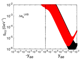
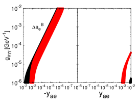
Figure 1: ALP-1: The 1$\sigma$ regions preferred by $\Delta a_{\mu}$, $\Delta a^{\rm LKB}_{e}$, and $\Delta a^{\rm B}_{e}$ for $m_{a}=1$ GeV (black) and $m_{a}=0.2$ GeV (red).

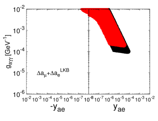
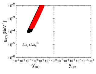
Figure 2: ALP-1: The 1$\sigma$ allowed regions from a combined fit to $\Delta a_{\mu}$ and $\Delta a^{\rm LKB}_{e}$ (upper panels) and $\Delta a_{\mu}$ and $\Delta a^{\rm B}_{e}$ (lower panels), for $m_{a}=1$ GeV (black) and $m_{a}=0.2$ GeV (red).

The minimum $\chi^{2}$ value in all cases is zero indicating that the deviations from the SM predictions can be exactly reproduced. Since the $\chi^{2}$ distributions are very shallow around the minima, we do do not provide best-fit ALP points.

In the left panel of Fig. 1, the plateau for small Yukawa couplings arises from the LbL contribution. For large negative $y_{a\mu}$, the BZ and 1-loop contributions interfere destructively with the LbL contribution which requires large $g_{a\gamma\gamma}$ values excluded by beam-dump experiments. For large positive $y_{a\mu}$ the BZ and LbL contributions interfere constructively so that the size of $g_{a\gamma\gamma}$ is reduced to fit the data. However, as $y_{a\mu}$ increases, the 1-loop contribution interferes destructively with the BZ and LbL contributions, which causes $g_{a\gamma\gamma}$ to rise again. A similar reasoning explains the structure of the $a_{e}^{\rm LKB}$ allowed region. A plateau does not appear in the allowed region for $\Delta a_{e}^{\rm B}$ because it is negative.

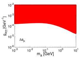
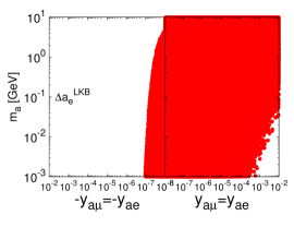
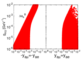
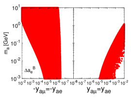
Figure 3: ALP-2: The 1$\sigma$ regions preferred by $\Delta a_{\mu}$ (upper panels), $\Delta a^{\rm LKB}_{e}$ (middle panels), and $\Delta a^{\rm B}_{e}$ (lower panels) for $y_{a\mu}=y_{ae}$.

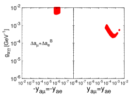
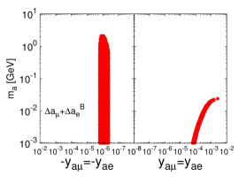
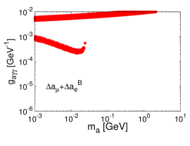
Figure 4: ALP-2: The 1$\sigma$ allowed regions from a combined fit to $\Delta a_{\mu}$ and $\Delta a^{\rm LKB}_{e}$ (upper panels) and $\Delta a_{\mu}$ and $\Delta a^{\rm B}_{e}$ (lower panels), for $y_{a\mu}=y_{ae}$.

3 Two-Higgs-doublet models

We now consider two-Higgs-doublet models. In addition to the light Higgs $h$, the scalar sector is comprised of a heavy Higgs $H$, pseudoscalar $A$, and two charge Higgses $H^{\pm}$, which contribute to the electron and muon $g-2$ through either 1-loop triangle diagrams or two-loop BZ diagrams. There are five relevant parameters, $m_{A}$, $m_{H}$, $m_{H^{\pm}}$, $\beta$, and $\alpha$. The ratio of the vacuum expectation values of the two scalar doublets $\Phi_{1,2}$ defines $\tan\beta\equiv v_{2}/v_{1}$. The mixing between the CP-even neutral components $h_{1,2}$ of $\Phi_{1,2}$, and the mass eigenstates $h,H$ is given by the angle $\alpha$ Branco:2011iw :

$$h = h_{1}\sin\alpha-h_{2}\cos\alpha\,,$$

$$H = -h_{1}\cos\alpha-h_{2}\sin\alpha\,.$$ (9)

To satisfy the stringent constraints on flavor changing neutral currents, the up-type quarks, down-type quarks and leptons must have Yukawa couplings to $\Phi_{1}$ or $\Phi_{2}$, but not both. This requirement leads to four types of 2HDMs: Type-I (all fermions couple to $\Phi_{2}$), Type-II (only up-type quarks couple to $\Phi_{2}$), Type-X (lepton-specific, in which only leptons couples to $\Phi_{2}$), Type-Y (flipped, in which only down-type quarks couples to $\Phi_{1}$) Branco:2011iw ; Chun:2015xfx . The rare decay $b\to s\gamma$ requires $m_{H^{\pm}}\gtrsim 300$ GeV for $\tan\beta\raisebox{-3.69899pt}{~{}\shortstack{$>$ \\ [-0.07cm] $\sim$}}~{}2$ for Type-I and Type-X Branco:2011iw ($m_{H^{\pm}}\gtrsim 580$ GeV for Type-II and Type-Y Misiak:2017bgg ), which renders their contributions to $g-2$ subdominant. Higgs precision measurements from ATLAS and CMS prefer $h$ to be SM-like with $\cos(\beta-\alpha)\to 0$, and $H$ decoupled. After fixing $m_{h}=125.5$ GeV, we are left with only two parameters $m_{A}$ and $\tan\beta$ that affect $g-2$. The Yukawa interactions in four types of 2HDMs are dictated by $\tan\beta$:

$$-\mathcal{L}_{\rm 2HDM}^{\rm Yukawa} = \sum_{f=u,d,\ell}\frac{m_{f}}{v_{\rm EW}}(y^{h}_{f}h\bar{f}f+y^{H}_{f}H\bar{f}f-iy^{A}_{f}\bar{f}\gamma_{5}f)$$ (10)

$$+ \left[\sqrt{2}V_{ud}H^{+}\bar{u}\left(\frac{m_{u}}{v_{\rm EW}}y^{A}_{u}P_{L}+\frac{m_{d}}{v_{\rm EW}}y^{A}_{d}P_{R}\right)d+\frac{\sqrt{2}m_{\ell}}{v_{\rm EW}}H^{+}\bar{\nu}P_{R}\ell+h.c.\right]\,,$$

with the normalized Yukawa couplings as listed in Table 1. The contribution to the anomalous magnetic moments is Chun:2015xfx

$$a_{\ell,\rm 2HDM}=a_{\ell,\rm 2HDM}^{\rm 1-loop}+a_{\ell,\rm 2HDM}^{\rm BZ}\,,\ \ \ {\text{where}}$$ (11)

$$a_{\ell,\rm 2HDM}^{\rm 1-loop}=\frac{G_{F}m^{2}_{\ell}}{4\pi^{2}\sqrt{2}}\sum_{j=\left\{h,H,A,H^{\pm}\right\}}(y^{j}_{\ell})^{2}r^{j}_{\ell}f_{j}(r^{j}_{\ell})\,,$$

$$a_{\ell,\rm 2HDM}^{\rm BZ}=\frac{G_{F}m^{2}_{\ell}}{4\pi^{2}\sqrt{2}}\frac{\alpha}{\pi}\sum_{i=\left\{h,H,A\right\};f=\left\{t,b,\tau\right\}}N^{c}_{f}Q^{2}_{f}y^{i}_{\ell}y^{i}_{f}r^{i}_{f}g_{i}(r^{i}_{f})\,,$$

where $r^{j}_{\ell}\equiv m^{2}_{\ell}/m^{2}_{j}$, $r^{i}_{f}\equiv m^{2}_{f}/m^{2}_{i}$, and $m_{f}$, $Q_{f}$, $N^{c}_{f}$ are the mass, electric charge and color factor for fermion $f$ in the loop. The loop functions are

$$f_{h,H}(r) = \int^{1}_{0}dx\frac{x^{2}(2-x)}{1-x+rx^{2}}\,,$$

$$f_{H^{\pm}}(r) = \int^{1}_{0}dx\frac{-x(1-x)}{1-r(1-x)}\,,$$

$$g_{h,H}(r) = \int^{1}_{0}dx\frac{2x(1-x)-1}{x(1-x)-r}\ln\frac{x(1-x)}{r}\,,$$

$$g_{A}(r) = \int^{1}_{0}dx\frac{1}{x(1-x)-r}\ln\frac{x(1-x)}{r}\,,$$ (12)

and $f_{A}(r)$ is same as in Eq. (7). The results of our statistical analysis by taking $\cos(\beta-\alpha)=0$ and $m_{H}=m_{H^{\pm}}=300$ GeV for Type-I and Type-X, and $m_{H}=m_{H^{\pm}}=580$ GeV for Type-II and Type-Y, are shown in Figs. 5, 6, 7, 8, and Table 2.

Not surprisingly, the Type-I model does not reproduce the data because it is similar to the SM. Type-Y is similar to Type-I except that the bottom quark contribution is enhanced. However, because of the lightness of the bottom quark, its contribution is not enough for the Type-Y model to explain the data. For Type-X, the large value of $\tan\beta$ enhances the tau-lepton contribution to the two-loop BZ diagram. The contribution from the bottom-quark in the BZ diagram provides a further enhancement in the Type-II model. Note that the Type-II parameters needed are excluded by constraints from $B_{s}\to\mu^{+}\mu^{-}$ and searches for $Z\to b\bar{b}A(b\bar{b})$ Chun:2015xfx .

Table 1: The normalized Yukawa couplings for the two-Higgs-doublet models Branco:2011iw .

$y^{A}_{u}$ $y^{A}_{d}$ $y^{A}_{\ell}$ $y^{H}_{u}$ $y^{H}_{d}$ $y^{H}_{\ell}$ $y^{h}_{u}$ $y^{h}_{d}$ $y^{h}_{\ell}$ Type-I $\cot\beta$ $-\cot\beta$ $-\cot\beta$ $\frac{\sin\alpha}{\sin\beta}$ $\frac{\sin\alpha}{\sin\beta}$ $\frac{\sin\alpha}{\sin\beta}$ $\frac{\cos\alpha}{\sin\beta}$ $\frac{\cos\alpha}{\sin\beta}$ $\frac{\cos\alpha}{\sin\beta}$ Type-II $\cot\beta$ $\tan\beta$ $\tan\beta$ $\frac{\sin\alpha}{\sin\beta}$ $\frac{\cos\alpha}{\cos\beta}$ $\frac{\cos\alpha}{\cos\beta}$ $\frac{\cos\alpha}{\sin\beta}$ $-\frac{\sin\alpha}{\cos\beta}$ $-\frac{\sin\alpha}{\cos\beta}$ Type-X $\cot\beta$ $-\cot\beta$ $\tan\beta$ $\frac{\sin\alpha}{\sin\beta}$ $\frac{\sin\alpha}{\sin\beta}$ $\frac{\cos\alpha}{\cos\beta}$ $\frac{\cos\alpha}{\sin\beta}$ $\frac{\cos\alpha}{\sin\beta}$ $-\frac{\sin\alpha}{\cos\beta}$ Type-Y $\cot\beta$ $\tan\beta$ $-\cot\beta$ $\frac{\sin\alpha}{\sin\beta}$ $\frac{\cos\alpha}{\cos\beta}$ $\frac{\sin\alpha}{\sin\beta}$ $\frac{\cos\alpha}{\sin\beta}$ $-\frac{\sin\alpha}{\cos\beta}$ $\frac{\cos\alpha}{\sin\beta}$

Figure 5: Type-I 2HDM: The 1$\sigma$ region preferred by $\Delta a^{\rm B}_{e}$. There is no solution for $\Delta a_{\mu}$ or $\Delta a^{\rm LKB}_{e}$ with $\chi^{2}<6.18$ (corresponding to $2\sigma$ for two parameters).

Figure 6: Type-II 2HDM: The 1$\sigma$ regions preferred by $\Delta a_{\mu}$, $\Delta a^{\rm{LKB}}_{e}$, and a combined fit of $\Delta a_{\mu}$ and $\Delta a^{\rm{LKB}}_{e}$. There is no solution for $\Delta a^{\rm B}_{e}$ with $\chi^{2}<6.18$.

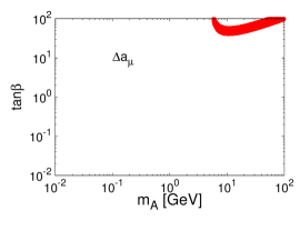
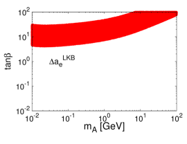
Figure 7: Type-X 2HDM: The 1$\sigma$ regions preferred by $\Delta a_{\mu}$, $\Delta a^{\rm{LKB}}_{e}$, and a combined fit of $\Delta a_{\mu}$ and $\Delta a^{\rm{LKB}}_{e}$. There is no solution for $\Delta a^{\rm B}_{e}$ with $\chi^{2}<6.18$.

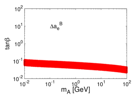
Figure 8: Type-Y 2HDM: The 1$\sigma$ region preferred by $\Delta a^{\rm B}_{e}$. There is no solution for $\Delta a_{\mu}$ or $\Delta a^{\rm LKB}_{e}$ with $\chi^{2}<6.18$.

Table 2: Best-fit points, their contributions to the anomalous magnetic moments, and minimum $\chi^{2}$ values for the 2HDMs.

Type-I Type-II Type-X Type-Y LKB B LKB B LKB B LKB B $m_{A}/{\rm GeV}$ 98.5 98.5 3.44 99.2 6.52 71.5 99.8 99.8 $\tan\beta$ 99.4 99.4 40.9 88.1 68.9 99.3 94.3 94.3 $a_{\mu}$ $-1.5\times 10^{-11}$ $-1.5\times 10^{-11}$ $2.5\times 10^{-9}$ $2.4\times 10^{-9}$ $2.5\times 10^{-9}$ $2.5\times 10^{-9}$ $-1.6\times 10^{-11}$ $-1.6\times 10^{-11}$ $a_{e}$ $-3.6\times 10^{-16}$ $-3.6\times 10^{-16}$ $4.8\times 10^{-13}$ $5.8\times 10^{-14}$ $4.9\times 10^{-13}$ $6.5\times 10^{-14}$ $-3.7\times 10^{-16}$ $-3.7\times 10^{-16}$ $\chi^{2}_{\rm LKB}$ 20.9 - $0$ - $0$ - 20.9 - $\chi^{2}_{\rm B}$ - 24.3 - 6.81 - 6.90 - 24.3

4 Leptoquarks

We consider a scalar leptoquark $S_{1}\sim({\bf 3},{\bf 1},-1/3)$ and a doublet leptoquark $(R_{2})^{T}=(R^{5/3}_{2},R^{2/3}_{2})\sim({\bf 3},{\bf 2},7/6)$. Their couplings to quarks and leptons are specified in the “up-type” mass-diagonal basis because the “down-type” basis would violate constraints from $\mu\to e\gamma$ Dorsner:2020aaz . Then, the CKM matrix appears in the couplings with down-type quarks, and the interaction Lagrangian is Bigaran:2020jil

$$\mathcal{L}^{S_{1}}\supset y^{SLQ}_{ij}\left[\bar{e}^{c}_{L,i}u_{L,j}-V^{\rm CKM}_{jk}\bar{\nu}^{c}_{L,i}d_{L,k}\right]S^{\dagger}_{1}+y^{Seu}_{ij}\bar{e}^{c}_{R,i}u_{R,j}S^{\dagger}_{1}+h.c.\,,$$

$$\mathcal{L}^{R_{2}}\supset y^{RLu}_{ij}\left[\bar{\nu}_{L,i}u_{R,j}R^{2/3,\dagger}_{2}-\bar{e}_{L,i}u_{R,j}R^{5/3,\dagger}_{2}\right]+y^{ReQ}\bar{e}_{R,i}\left[u_{L,j}R^{5/3,\dagger}_{2}+V^{\rm CKM}_{jk}d_{L,k}R^{2/3,\dagger}_{2}\right]+h.c.$$

$S_{1}$ and $R^{5/3}_{2}$ have left- and right-handed couplings to the charge leptons and up-type quarks, and give a large contribution to $a_{\ell}$ under the condition $m_{q}\gg m_{\ell}$. We neglect the contribution of $R^{2/3}_{2}$, which only has right-handed couplings to down quarks. In the limit, $m_{q}\ll m_{\rm LQ}$,

$$a_{\ell,S_{1}}\simeq-\frac{m_{\ell}m_{q}}{4\pi^{2}m^{2}_{S_{1}}}\left[\frac{7}{4}-2\log\left(\frac{m_{S_{1}}}{m_{q}}\right)\right]{\rm Re}(y^{L*}_{\ell q}y^{R}_{\ell q})\,,$$

$$a_{\ell,R_{2}}\simeq\frac{m_{\ell}m_{q}}{4\pi^{2}m^{2}_{R_{2}}}\left[\frac{1}{4}-2\log\left(\frac{m_{R_{2}}}{m_{q}}\right)\right]{\rm Re}(y^{L*}_{\ell q}y^{R}_{\ell q})\,,$$ (14)

where for $S_{1}$, $y^{R}_{ij}\equiv y^{Seu}_{ij}$ and $y^{L}_{ij}\equiv y^{SLQ}_{ij}$; and for $R^{5/3}_{2}$, $y^{R}_{ij}\equiv-y^{RLu}_{ij}$ and $y^{L}_{ij}\equiv y^{ReQ}_{ij}$. Note that $a_{\ell}$ requires both non-vanishing left- and right-handed Yukawa couplings. There is freedom to choose the texture of the Yukawa couplings $y^{L,R}_{ij}$. According to Eq. (4), heavier fermions contribute more to $a_{\ell}$, so we ignore the $u$ quark and $\tau$ lepton. The remaining couplings are $y^{L,R}_{ec,\,et,\,\mu c,\,\mu t}$. However, if both $y_{et}$ and $y_{\mu t}$ are non-zero, the $m_{t}$ enhancement of $\mu\to e\gamma$ becomes incompatible with observation Bigaran:2020jil . A non-zero $y_{\mu c}$ allows the LQ to couple to neutrinos and the $s$ quark, thereby inducing $K^{+}\to\pi^{+}\nu\nu$ through CKM mixing. To obey these constraints we set $y_{et}=y_{\mu c}=0$. Finally, we have the Yukawa couplings,

$$y^{L}_{ij}\sim\left(\begin{array}[]{ccc}0&y^{L}_{ec}&0\\[5.69054pt] 0&0&y^{L}_{\mu t}\\[5.69054pt] 0&0&0\end{array}\right),~{}~{}~{}~{}y^{R}_{ij}\sim\left(\begin{array}[]{ccc}0&y^{R}_{ec}&0\\[5.69054pt] 0&0&y^{R}_{\mu t}\\[5.69054pt] 0&0&0\end{array}\right)\,.$$ (21)

Taking the couplings to be real, we scan the parameter space in two scenarios:

• $S_{1}$-LQ: We fix $m_{S_{1}}=2$, 10 TeV, and vary $y^{L}_{ec}y^{R}_{ec}$ and $y^{L}_{\mu t}y^{R}_{\mu t}$. The results are shown in Fig. 9 and Table 3.

• $R_{2}$-LQ: fixing $m_{R_{2}}=2$, 10 TeV, and varying $y^{L}_{ec}y^{R}_{ec}$, and $y^{L}_{\mu t}y^{R}_{\mu t}$. The results are shown in Fig. 10 and Table 3.

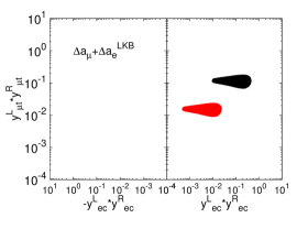
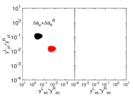
Figure 9: $S_{1}$-LQ: The 1$\sigma$ regions preferred by $\Delta a_{\mu}$, $\Delta a^{\rm LKB}_{e}$, and $\Delta a^{\rm B}_{e}$ (upper panels), and from a combined fit to $\Delta a_{\mu}$ and $\Delta a^{\rm LKB}_{e}$, and $\Delta a_{\mu}$ and $\Delta a^{\rm B}_{e}$ (lower panels), for $m_{S_{1}}=10$ TeV (black) $m_{S_{1}}=2$ TeV (red).

Table 3: Best-fit points for the scalar and doublet leptoquarks. The minimum $\chi^{2}$ value in all cases is 0.

$S_{1}$-LQ $R_{2}$-LQ LKB LKB B B LKB LKB B B $m_{S_{1}(R_{2})}/{\rm TeV}$ 2 10 2 10 2 10 2 10 $y^{L}_{ec}y^{R}_{ec}$ $1.1\times 10^{-2}$ 0.20 $-1.9\times 10^{-2}$ -0.37 $-8.3\times 10^{-3}$ -0.16 $1.5\times 10^{-2}$ 0.30 $y^{L}_{\mu t}y^{R}_{\mu t}$ $1.6\times 10^{-2}$ 0.12 $1.5\times 10^{-2}$ 0.12 $-4.7\times 10^{-3}$ $-6.9\times 10^{-2}$ $-4.7\times 10^{-3}$ $-6.8\times 10^{-2}$

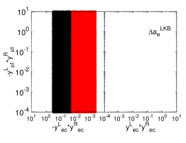
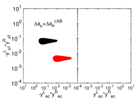
Figure 10: $R_{2}$-LQ: The 1$\sigma$ regions preferred by $\Delta a_{\mu}$, $\Delta a^{\rm LKB}_{e}$, and $\Delta a^{\rm B}_{e}$ (upper panels), and from a combined fit to $\Delta a_{\mu}$ and $\Delta a^{\rm LKB}_{e}$, and $\Delta a_{\mu}$ and $\Delta a^{\rm B}_{e}$ (lower panels), for $m_{R_{2}}=10$ TeV (black) $m_{R_{2}}=2$ TeV (red).

5 Summary

In light of the recent measurement of the muon anomalous magnetic moment by the Muon g-2 experiment, we examine three model frameworks as explanations of the $(g-2)_{e,\mu}$ discrepancy with standard model expectations. We considered i) axion-like particles with masses $\lesssim\mathcal{O}(1)$ GeV and couplings to charged leptons and photons, which yields a contribution to the 2-loop light-by-light diagram for $(g-2)_{e,\mu}$. ii) Two-Higgs-doublet models with four Yukawa structures: Type-I, II, X (lepton-specific), and Y (flipped), where the CP-odd scalar with mass $\lesssim\mathcal{O}(100)$ GeV gives the main contribution to $(g-2)_{e,\mu}$ up to 2-loop Barr-Zee diagrams. iii) Scalar leptoquarks, $S_{1}\sim({\bf 3},{\bf 1},-1/3)$ and $R_{2}\sim({\bf 3},{\bf 2},7/6)$, where the Yukawa couplings are assigned as up-type mass-diagonal basis to avoid constraints from $\mu\to e\gamma$. Then the mixed-chiral charm-electron and top-muon Yukawa couplings contribute to $(g-2)_{e}$ and $(g-2)_{\mu}$, respectively.

We find that accounting for other constraints, all scenarios except the Type-I, Type-II and Type-Y two-Higgs-doublet models easily accommodate the data.

References

- (1) G. W. Bennett et al. [Muon g-2 Collaboration], Phys. Rev. D 73, 072003 (2006), [hep-ex/0602035].
- (2) P. A. Zyla et al. [Particle Data Group], PTEP 2020, no. 8, 083C01 (2020).
- (3) T. Aoyama, N. Asmussen, M. Benayoun, J. Bijnens, T. Blum, M. Bruno, I. Caprini, C. M. Carloni Calame, M. Cè and G. Colangelo, et al. Phys. Rept. 887, 1-166 (2020) [arXiv:2006.04822 [hep-ph]].
- (4) S. Borsanyi, Z. Fodor, J. N. Guenther, C. Hoelbling, S. D. Katz, L. Lellouch, T. Lippert, K. Miura, L. Parato and K. K. Szabo, et al. [arXiv:2002.12347 [hep-lat]].
- (5) B. Abi et al. [Muon g-2], Phys. Rev. Lett. 126, 141801 (2021) [arXiv:2104.03281 [hep-ex]].
- (6) L. Morel, Z. Yao, P. Cladé and S. Guellati-Khélifa, Nature 588, no. 7836, 61 (2020).
- (7) R. H. Parker, C. Yu, W. Zhong, B. Estey and H. Müller, Science 360, 191 (2018), [arXiv:1812.04130 [physics.atom-ph]].
- (8) T. Aoyama, M. Hayakawa, T. Kinoshita and M. Nio, Phys. Rev. Lett. 109, 111807 (2012), [arXiv:1205.5368 [hep-ph]].
- (9) T. Aoyama, T. Kinoshita and M. Nio, Atoms 7, no. 1, 28 (2019).
- (10) D. Hanneke, S. Fogwell and G. Gabrielse, Phys. Rev. Lett. 100, 120801 (2008), [arXiv:0801.1134 [physics.atom-ph]].
- (11) F. Jegerlehner and A. Nyffeler, Phys. Rept. 477, 1 (2009), [arXiv:0902.3360 [hep-ph]].
- (12) J. Prades, arXiv:0907.2938 [hep-ph].
- (13) A. E. Dorokhov, A. E. Radzhabov and A. S. Zhevlakov, Eur. Phys. J. C 75, no. 9, 417 (2015), [arXiv:1502.04487 [hep-ph]].
- (14) J. D. Bjorken and S. Weinberg, Phys. Rev. Lett. 38, 622 (1977); S. M. Barr and A. Zee, Phys. Rev. Lett. 65, 21-24 (1990) [erratum: Phys. Rev. Lett. 65, 2920 (1990)]
- (15) E. J. Chun, EPJ Web Conf. 118, 01006 (2016) [Pramana 87, no. 3, 41 (2016)], [arXiv:1511.05225 [hep-ph]].
- (16) W. J. Marciano, A. Masiero, P. Paradisi and M. Passera, Phys. Rev. D 94, no. 11, 115033 (2016), [arXiv:1607.01022 [hep-ph]].
- (17) J. Jaeckel and M. Spannowsky, Phys. Lett. B 753, 482 (2016), [arXiv:1509.00476 [hep-ph]].
- (18) K. Mimasu and V. Sanz, JHEP 1506, 173 (2015) [arXiv:1409.4792 [hep-ph]].
- (19) G. C. Branco, P. M. Ferreira, L. Lavoura, M. N. Rebelo, M. Sher and J. P. Silva, Phys. Rept. 516, 1 (2012), [arXiv:1106.0034 [hep-ph]].
- (20) M. Misiak and M. Steinhauser, Eur. Phys. J. C 77, no.3, 201 (2017) [arXiv:1702.04571 [hep-ph]].
- (21) I. Doršner, S. Fajfer and S. Saad, Phys. Rev. D 102, no. 7, 075007 (2020), [arXiv:2006.11624 [hep-ph]].
- (22) I. Bigaran and R. R. Volkas, Phys. Rev. D 102, no. 7, 075037 (2020), [arXiv:2002.12544 [hep-ph]].