Design of MIMO Radar Waveforms based on $\ell_{p}$-Norm Criteria

Abstract

Multiple-input multiple-output (MIMO) radars transmit a set of sequences that exhibit small cross-correlation sidelobes, to enhance sensing performance by separating them at the matched filter outputs. The waveforms also require small auto-correlation sidelobes to avoid masking of weak targets by the range sidelobes of strong targets and to mitigate deleterious effects of distributed clutter. In light of these requirements, in this paper, we design a set of phase-only (constant modulus) sequences that exhibit near-optimal properties in terms of Peak Sidelobe Level (PSL) and Integrated Sidelobe Level (ISL). At the design stage, we adopt weighted $\ell_{p}$-norm of auto- and cross-correlation sidelobes as the objective function and minimize it for a general $p$ value, using block successive upper bound minimization (BSUM). Considering the limitation of radar amplifiers, we design unimodular sequences which make the design problem non-convex and NP-hard. To tackle the problem, in every iteration of the BSUM algorithm, we introduce different local approximation functions and optimize them concerning a block, containing a code entry or a code vector. The numerical results show that the performance of the optimized set of sequences outperforms the state-of-the-art counterparts, in both terms of PSL values and computational time.

I Introduction

A complex problem in radar pulse compression (intra-pulse modulation) is the design of waveforms exhibiting small Peak Sidelobe Level (PSL). PSL shows the maximum auto-correlation sidelobe of a transmit waveform in a typical Single-Input Single-Output (SISO)/Single-Input Multiple-Output (SIMO), or phased-array radar system. If this value is not small, then either a false detection or a miss detection may happen, based on the way the Constant False Alarm Rate (CFAR) detector is tuned [1]. In Multiple-Input Multiple-Output (MIMO) radars, PSL minimization is more complex since the cross-correlation sidelobes of transmitting set of sequences need to be also considered. Small value in cross-correlation sidelobes helps the radar receiver to separate the transmitting waveforms and form a MIMO virtual array.

Similar properties hold for Integrated Sidelobe Level (ISL) of transmitting waveforms where in case of SISO/SIMO or phased-array radars, the energy of auto-correlation sidelobes should be small to mitigate the deleterious effects of distributed clutter. In solid state-based weather radars, ISL needs to be small to enhance reflectively estimation and improve the performance of hydrometer classifier [2]. In MIMO radar systems, ISL shows the energy leakage of different waveforms in addition to the energy of non-zero auto-correlation sidelobes. Indeed, correlation sidelobes are a form of self-noise that reduce the effectiveness of transmitting waveforms in every radar system [3].

In a MIMO radar system, different multiplexing schemes can be used to create zero values for cross-correlations of the transmitting waveforms, Frequency Division Multiplexing (FDM), Doppler Division Multiplexing (DDM), and Time Division Multiplexing (TDM) as some examples [4]. Currently, TDM-MIMO radars are commercialized in the automotive industry with a variety of functionalities from de-chirping and Doppler processing to angle estimation and tracking [5, 6]. However, Code Division Multiplexing (CDM)-MIMO is the next step of the industry, which can use more efficiently the available resources (time and frequency) [7].

In this paper, we devise a method called Weighted BSUM sEquence SeT (WeBEST) to design transmitting waveforms for CDM-MIMO radars. To this end, we adopt the weighted $\ell_{p}$-norm of auto- and cross-correlation sidelobes as the objective function and minimize it under Continuous Phase (CP) and Discrete Phase (DP) constraints. The weighting and $p$ values in the provided formulation create a possibility for intelligent transmission based on prevailing environmental conditions, where can select appropriate $p$ based on presence of distributed clutter or strong target [8, 9, 10, 11]. For example, choosing $p\to 0$ and minimizing the $\ell_{p}$-norm of auto- and cross-correlation sidelobes, a set of sequences with sparse sidelobes will be obtained. With $p=2$, the resulting optimized set of sequences will have small ISL value which performs well in the presence of clutter. Further, by minimizing the $\ell_{p}$-norm when $p\rightarrow+\infty$, the optimized set of sequence will have small PSL and are well suited for enhancing the detection of point targets.

I-A Background and Related Works

Waveform design based on sidelobe reduction in SISO/SIMO or phased-array radar systems: Research into design of waveforms with small ISL and PSL values has significantly increased over the past decade for single waveform transmitting radar systems [12, 13, 14, 15, 16, 17, 18, 19, 20]. In case of ISL minimization, several optimization frameworks are proposed, including power method-like iterations, Majorization-Minimization (MM), Coordinate Descent (CD), Gradient Descent (GD) and Alternating Direction Method of Multipliers (ADMM) to name a few [12, 13, 14, 15, 17, 16, 18, 19, 20]. Further, joint ISL and PSL minimization based on CD under DP and CP constraints is proposed in [18]. In this paper $\ell_{p}$-norm of auto-correlation sidelobes when $p\rightarrow+\infty$ is considered for the initialization. Similarly, several papers have considered $\ell_{p}$-norm minimization to design waveform with small PSL values. In [15, 16], MM based approach are proposed for $\ell_{p}$-norm minimization when $p\geq 2$. Also, the authors in [19] proposed a GD based approach for $\ell_{p}$-norm minimization when $p$ is an even number, i.e., $p=2n,n\in\mathbb{Z}^{+}$. The results in [18] depict that a methodology based on the $\ell_{p}$-norm of auto-correlation sidelobes by gradually increasing $p$, provides sequences with smaller PSL values comparing with the direct minimization of the PSL. Motivated by this observation, this paper investigates $\ell_{p}$-norm minimization of auto- and cross-correlation functions to obtain set of sequences with very small PSL values for MIMO radar systems.

Waveform design based on sidelobe reduction in MIMO radar systems: In order to design set of sequences with small auto- and cross-correlation sidelobes, several approaches including Multi-Cyclic Algorithm-New (CAN)/Multi-PeCAN [21], Iterative Direct Search [22], ISL New [23], MM-Corr [24] and CD [25, 26], are proposed all considering the ISL as the design metric. On the other hand, few papers have focused on PSL minimization for MIMO radars [27, 28]. In [27] a CD based approach is proposed to directly minimize a weighted sum of PSL and ISL for MIMO radars under DP constraint. In [28] a MM based approach is proposed to directly minimize the PSL and design set of sequences for MIMO radar systems. In the current study, we design set of sequences with very small PSL values by minimizing $\ell_{p}$-norm of auto- and cross-correlation sidelobes for a set of sequences which was not addressed previously in the literature. In contrast to the previous studies, we solve the problem for a general $p$ value ($p>0$) under DP constraint, and solve it for $p\in(0,1]\cup p\geq 2$ under CP constraint. Interestingly, the obtained PSL values are close to the welch lower bound and fill the gap between the best of literature and the lower bound. TABLE I compares the contributions of the proposed WeBEST method with the state-of-the art approaches.

TABLE I: The difference of the proposed method with the state of the art.

Paper	PSL	ISL	$\ell_{p}$-norm	type	weight
[18]	✓	✓	$p\geq 2$	SISO	$\times$
[15, 16]	✓	✓	$p\geq 2$	SISO	✓
[12]	$\times$	✓	$\times$	SISO	✓
[13, 20, 17]	$\times$	✓	$\times$	SISO	$\times$
[19]	✓	✓	$p\geq 2$ for $p$ even	SISO	✓
[21, 22, 23, 24, 25, 26]	$\times$	✓	$\times$	MIMO	✓
[27]	✓	✓	$\times$	MIMO	$\times$
[28]	✓	$\times$	$\times$	MIMO	$\times$
WeBEST (DP)	✓	✓	$p>0$	MIMO	✓
WeBEST (CP)	✓	✓	$p\in(0,1]\cup p\geq 2$	MIMO	✓

I-B Contributions

The main contributions of the current article are summarized below.

• Unified optimization framework: We propose a unified framework based on Block Successive Upper Bound Minimization (BSUM) paradigm to solve a general $\ell_{p}$-norm of auto- and cross-correlation minimization problem under practical waveform design constraints which make the problem non-convex, non-smooth and NP-hard. While BSUM offers a generic framework, the contribution of the paper lies in devising different solutions based on implementation complexity and performance under a unified framework that solves the problem. The proposed problem formulation includes $\ell_{1}$/$\ell_{0}$-norm of the auto-correlation sidelobe which relatively have lower number of local minima comparing with $l_{2}$-norm. Also, the local minima of those cost function would correspond to sequences with good auto-correlation sidelobe levels. For instance, in the simulation analysis we show that any local minima of $\ell_{0}$-norm of auto-correlation would have many zeros (sparse auto-correlation) which can enhance the detection performance in the presence of distributed clutter.

• Entry- and vector-based solutions: In each iteration of BSUM, we propose two approaches, i.e, entry- and vector-based solutions. In the entry-based optimization, we formulate the problem with respect to a single variable; this enable us to find the critical points and obtain the global optimum solution in each step. For vector-based optimization we propose a solution based on GD. This approach is faster than the entry-based method. However, the entry-based method has a better performance in terms of minimizing the objective function due to obtaining the global optimum solution in each step.

• Trade-off and flexibility: By conducting thorough performance assessment, we propose a flexible tool to design set of sequences with different properties. We show that the $\ell_{p}$-norm optimization framework provides the flexibly of controlling optimization objective by choosing $p$, where $p\to\infty$ leads to design set of waveforms with good PSL property. Choosing $p\to 0$ leads to sparse auto- and cross-correlation and choosing $p=2$ leads to design set of waveforms with good ISL property.

We finally propose a direct solution for the discrete phase constraint using Fast Fourier Transform (FFT)-based technique.

I-C Organization and Notations

The rest of this paper is organized as follows. In Section II, we formulate the $\ell_{p}$-norm minimization for MIMO radar systems, then we introduce the BSUM method as the Optimization framework and finally we define the local approximation functions suitable for $\ell_{p}$-norm problem. We develop the BSUM framework to solve the problem in Section III and provide numerical experiments to verify the effectiveness of proposed algorithm in Section IV.

Notations

This paper uses lower-case and upper-case boldface for vectors ($a$) and matrices ($A$) respectively. The set of complex and positives integer numbers are denoted by $\mathbb{C}$ and $\mathbb{Z}^{+}$ respectively. The transpose, conjugate transpose and sequence reversal are denoted by the $(.)^{T}$, $(.)^{H}$ and $(.)^{r}$ symbols respectively. Besides the Frobenius norm, $\ell_{p}$ norm, absolute value and round operator are denoted by $\mathinner{\!\left\lVert.\right\rVert}_{F}$, $\mathinner{\!\left\lVert.\right\rVert}_{p}$, $|.|$ and $\lfloor.\rceil$, respectively. For any complex number $a$, $\Re(a)$ and $\Im(a)$ denotes the real and imaginary part respectively. The letter $j$ represents the imaginary unit (i.e., $j=\sqrt{-1}$), while the letter $(i)$ is use as step of a procedure. Finally $\odot$ and $\circledast$ denotes the Hadamard product and cross-correlation operator respectively.

II Problem Formulation and Optimization Framework

We consider a narrow-band MIMO radar system with $M$ transmitters and each transmitting a sequence of length $N$ in the fast-time domain. Let the matrix $\mbox{\boldmath{$X$}}\in\mathbb{C}^{M\times N}$ denote the set of transmitted sequences in baseband, whose the $m^{th}$ row indicates the $N$ samples of $m^{th}$ transmitter while the $n^{th}$ column indicates the $n^{th}$ time-sample across the $M$ transmitters. Let $\mathbf{x}_{m}\triangleq[x_{m,1},x_{m,2},\dots,x_{m,N}]^{T}\in\mathbb{C}^{N}$ be the transmitted signal from $m^{th}$ transmitter. The aperiodic cross-correlation of $\mathbf{x}_{m}$ and $\mathbf{x}_{l}$ is defined as,

$$r_{m,l}(k)\triangleq(\mathbf{x}_{m}\circledast\mathbf{x}_{l})_{k}=\textstyle\sum_{n=1}^{N-k}x_{m,n}x_{l,n+k}^{*},$$ (1)

where $m,l\in\{1,\dots,M_{t}\}$ are the transmit antennas indices and $k\in\{-N+1,\dots,N-1\}$ is the lag of cross-correlation. If $m=l$, (1) represents the aperiodic auto-correlation of signal $\mathbf{x}_{m}$. The zero lag of auto-correlation ($r_{m,m}(0)$) represent the mainlobe of the matched filter output. Also $|r_{m,m}(0)|$ contains the energy of sequence which for constant modulus sequences is equal to $N$. The other lags ($k\neq 0$) are referred to the sidelobes. The weighted $\ell_{p}$-norm of auto- and cross correlation in MIMO radar can be written as,

$$\left(\textstyle\sum_{m=1}^{M}\sum_{l=1}^{M}\sum_{k=-N+1}^{N-1}|w_{k}r_{m,l}(k)|^{p}-M(w_{0}N)^{p}\right)^{\frac{1}{p}},$$ (2)

where, $0\leq w_{k}\leq 1$. The $M(w_{0}N)^{p}$ term in (2) is the weighted $\ell_{p}$-norm of the mainlobes, where $\sum_{m=1}^{M}|w_{0}r_{m,m}(0)|^{p}=M(w_{0}N)^{p}$. Since the term $M(w_{0}N)^{p}$ in (2) is constant, the weighted $\ell_{p}$-norm minimization can be equivalently written as,

$$\mathcal{P}\begin{dcases}\min_{\mbox{\boldmath{$X$}}}&f(\mbox{\boldmath{$X$}})\triangleq\textstyle\sum_{m=1}^{M}\sum_{l=1}^{M}\sum_{k=-N+1}^{N-1}|w_{k}r_{m,l}(k)|^{p}\\ s.t&x_{m,n}\in{\mathcal{X}}_{\infty}\quad\text{or}\quad{\mathcal{X}}_{L},\\ \end{dcases}$$ (3)

where, ${\mathcal{X}}_{\infty}$ and ${\mathcal{X}}_{L}$ indicating the unimodular and discrete phase with $L$ alphabet size sequences. More precisely, we consider $\mathcal{X}_{\infty}=\{e^{j\phi}|\phi\in\Omega_{\infty}\}$ and $\mathcal{X}_{L}=\{e^{j\phi}|\phi\in\Omega_{L}\}$, where $\Omega_{\infty}\triangleq(-\pi,\pi]$ and $\Omega_{L}\triangleq\{0,\frac{2\pi}{L}\,\dots,\frac{2\pi(L-1)}{L}\}$. The unimodular and discrete phase are equality constraint and they are not an affine set. Therefore the optimization problem not only is non-convex, but also multi-variable and NP-hard in general. Besides, due to the parameter $p$, in general dealing directly with $f(\mbox{\boldmath{$X$}})$ is complicated. In the following we introduce BSUM method to solve the optimization problem effectively.

II-A BSUM framework

The BSUM algorithm includes algorithms that successively optimize particular upper-bounds or local approximation functions of the original objectives in a block by block manner [29, 30, 31, 32]. Let $\mbox{\boldmath{$X$}}\triangleq[\mathbf{x}_{1}^{T};\dots;\mathbf{x}_{M}^{T}]\in\mathbb{C}^{M\times N}$, where $\mathbf{x}_{m},m=1,\dots,M$ is the transmitted signal from $m^{th}$ transmitter. The following optimization problem,

$$\begin{dcases}\min_{\mathbf{x}}&f(\mathbf{x}_{1},\mathbf{x}_{2},\ldots,\mathbf{x}_{M}),\\ \text{s.t.}&\mathbf{x}_{m}\in{\mathcal{X}}_{m},~{}m=1,\ldots,M.\end{dcases}$$ (4)

can be iteratively solved using the BSUM technique, by finding the solutions of the following sub-problems for $i=0,1,2,\ldots$,

$$\mathbf{x}_{1}^{(i+1)}= \arg{\min_{\mathbf{x}_{1}\in\mathcal{X}_{1}}}~{}~{}u_{1}(\mathbf{x}_{1},\mathbf{x}_{2}^{(i)},\mathbf{x}_{3}^{(i)},\ldots,\mathbf{x}_{M}^{(i)}),$$

$$\mathbf{x}_{2}^{(i+1)}= \arg{\min_{\mathbf{x}_{2}\in\mathcal{X}_{2}}}~{}~{}u_{2}(\mathbf{x}_{1}^{(i+1)},\mathbf{x}_{2},\mathbf{x}_{3}^{(i)},\ldots,\mathbf{x}_{M}^{(i)}),$$

$$\vdots$$

$$\mathbf{x}_{N}^{(i+1)}= \arg{\min_{\mathbf{x}_{M}\in\mathcal{X}_{M}}}~{}~{}u_{n}(\mathbf{x}_{1}^{(i+1)},\mathbf{x}_{2}^{(i+1)},\mathbf{x}_{3}^{(i+1)},\ldots,\mathbf{x}_{M}),$$

where $u_{n}$ is local approximation of the objective function. The BSUM procedure consists of three steps as follows,

• We select a block.

• We find a local approximation function that locally approximates the objective function.

• At every iteration $i$, a single block, say $m=(i~{}\text{mod}~{}M)+1$, is optimized by minimizing a approximation function of the selected block.

If at some point, the objective is not decreasing at every coordinate direction, then we have obtained the optimum $\mbox{\boldmath{$X$}}^{\star}\equiv\mbox{\boldmath{$X$}}^{(i+1)}\triangleq[{\mathbf{x}_{1}^{(i+1)}}^{T},{\mathbf{x}_{2}^{(i+1)}}^{T},\ldots,{\mathbf{x}_{M}^{(i+1)}}^{T}]$. The above framework is rather general, and leaves us the freedom of how to choose the index $m$ at $i$-th iteration.

II-B Choice of local approximation Functions

The local approximation functions play an important role to simplify and efficiently solve the optimization problem. In the following, we introduce some local approximation functions which reduce the weighted $\ell_{p}$-norm problem of (3) to simpler quadratic forms for $0<p\leq 1$ and $p\geq 2$.

II-B1 local approximation Function for $p\geq 2$

In this case, one choice for local approximation function is using majorization function [30]. Let $u(\mathbf{x})$ be a majorization (minorization) function of $f(\mathbf{x})$ and $\mathbf{x}^{(i)}$ be the variable at $i^{(th)}$ iteration. This function must satisfy the following conditions [33],

$$u(\mathbf{x}^{(i)})=f(\mathbf{x}^{(i)});\ \forall\mathbf{x}^{(i)}\in{\mathcal{X}}$$ (5a)

$$u(\mathbf{x})\geq f(\mathbf{x})\ (\text{minorize:}\ u(\mathbf{x})\leq f(\mathbf{x}));\ \forall\mathbf{x},\in{\mathcal{X}}$$ (5b)

$$\nabla u(\mathbf{x}^{(i)})=\nabla f(\mathbf{x}^{(i)});\ \forall\mathbf{x}^{(i)}\in{\mathcal{X}}$$ (5c)

$$u(\mathbf{x})\ \text{is continuous}\ \forall\mathbf{x},\in{\mathcal{X}}.$$ (5d)

When $p\geq 2$, $|w_{k}r_{m,l}(k)|^{p}$ can be majorized by the following function [15],

$$\eta_{mlk}|w_{k}r_{m,l}(k)|^{2}+\psi_{mlk}|w_{k}r_{m,l}(k)|+\nu_{mlk}$$ (6)

where,

$$\eta_{mlk} \triangleq\frac{\tau^{p}+(p-1)|w_{k}r_{m,l}^{(i)}(k)|^{p}-p\tau|w_{k}r_{m,l}^{(i)}(k)|^{(p-1)}}{(\tau-|w_{k}r_{m,l}^{(i)}(k)|)^{2}}$$ (7)

$$\psi_{mlk} \triangleq p|w_{k}r_{m,l}^{(i)}(k)|^{(p-1)}-2\eta_{mlk}|w_{k}r_{m,l}^{(i)}(k)|$$

$$\nu_{mlk} \triangleq\eta_{mlk}|w_{k}r_{m,l}^{(i)}(k)|^{2}-(p-1)|w_{k}r_{m,l}^{(i)}(k)|^{p}$$

and

$$\tau\triangleq\textstyle\left(\sum_{-N-1}^{N-1}|w_{k}r_{m,l}^{(i)}(k)|^{p}\right)^{\frac{1}{p}}$$ (8)

Furthermore, (6) can be majorized by [15],

$$u(w_{k}r_{m,l}(k)) \triangleq\eta_{mlk}|w_{k}r_{m,l}(k)|^{2}$$ (9)

$$+\psi_{mlk}\Re\left\{w_{k}^{*}r_{m,l}^{*}(k)\frac{w_{k}r_{m,l}^{(i)}(k)}{|w_{k}r_{m,l}^{(i)}(k)|}\right\}+\nu_{mlk}$$

Thus, the quadratic local approximation function of $f(\mbox{\boldmath{$X$}})$ for $p\geq 2$ is,

$$u(\mbox{\boldmath{$X$}})\triangleq\textstyle\sum_{m=1}^{M}\sum_{l=1}^{M}\sum_{k=-N+1}^{N-1}u(w_{k}r_{m,l}(k))$$ (10)

II-B2 local approximation Function for $0<p\leq 1$

$f(\mbox{\boldmath{$X$}})|_{p\to 0}$ denotes the number of non-zero elements of auto- and cross-correlation. In order to avoid the singularity problem to obtain the derivative of $f(\mbox{\boldmath{$X$}})$, we replace $f(\mbox{\boldmath{$X$}})|_{p\to 0}$ with smooth approximation functions $g_{h}(\mbox{\boldmath{$X$}})\triangleq\sum_{m=1}^{M}\sum_{l=1}^{M}\sum_{k=-N+1}^{N-1}g_{h}(w_{k}r_{m,l}(k))$, $h\in\{1,2,3\}$, where [34],

$$g_{1}(r_{m,l}(k)) \triangleq|w_{k}r_{m,l}(k)|^{p},\quad 0<p\leqslant 1,$$ (11)

$$g_{2}(r_{m,l}(k)) \triangleq\frac{\ln(1+\frac{|w_{k}r_{m,l}(k)|^{p}}{p})}{\ln(1+\frac{1}{p})},\quad p>0,$$

$$g_{3}(r_{m,l}(k)) \triangleq 1-e^{-\frac{|w_{k}r_{m,l}(k)|^{p}}{p}},\quad p>0.$$

The aforementioned smooth approximation functions may simplify the optimization problem, but they still have an order $p$. This means that is not yet easy to optimize the above smooth functions. To find a local approximation function, notice that each of the above smooth approximations can be majorized with the following simpler quadratic function [34],

$$v_{h}(w_{k}r_{m,l}(k))\triangleq\gamma_{hmlk}|w_{k}r_{m,l}(k)|^{2}+\mu_{hmlk}$$ (12)

where, the coefficients $\gamma_{hmlk}$ and $\mu_{hmlk}$ can be obtained by solving the following system of equation [34],

$$g_{h}(w_{k}r_{m,l}^{(i)}(k))= v_{h}(w_{k}r_{m,l}^{(i)}(k))$$ (13)

$$\frac{\partial g_{h}(w_{k}r_{m,l}^{(i)}(k))}{\partial|w_{k}r_{m,l}^{(i)}(k)|}= 2\gamma_{hmlk}|w_{k}r_{m,l}^{(i)}(k)|.$$

resulting in,

$$\mu_{hmlk}=g_{h}(w_{k}r_{m,l}^{(i)}(k))-\gamma_{h}|w_{k}r_{m,l}^{(i)}(k)|^{2}$$ (14)

$$\gamma_{hmlk}=\frac{\partial g_{h}(w_{k}r_{m,l}^{(i)}(k))}{\partial|w_{k}r_{m,l}^{(i)}(k)|}\times\frac{1}{2|w_{k}r_{m,l}^{(i)}(k)|},$$

The quadratic functions in (12), (14) are non-differentiable and singular when $w_{k}r_{m,l}(k)=0$. A solution suggested in [34] is to incorporate a small $\epsilon>0$ that avoids this singularity issue and use the smooth approximation functions $g_{h}^{\epsilon}(w_{k}r_{m,l}(k))$ and $\gamma_{hmlk}^{\epsilon}$ which are written in TABLE II. In this table, $\mu_{hmlk}^{\epsilon}$ is not reported, since it is a constant term and does not affect the optimization procedure.

TABLE II: The smooth approximation function of $l_{p}$-norm and correspond local approximation function when $0<p<1$

Smooth approximation functions ($g_{h}^{\epsilon}(w_{k}r_{m,l}(k))$)	Coefficients of majorization functions ($\gamma_{hmlk}^{\epsilon}$) (12)
$\begin{dcases}\frac{p}{2}\epsilon^{p-2}|w_{k}r_{m,l}(k)|^{2}&|w_{k}r_{m,l}(k)|\leqslant\epsilon\\ |w_{k}r_{m,l}(k)|^{p}-(1-\frac{1}{p})\epsilon^{p}&|w_{k}r_{m,l}(k)|>\epsilon\\ \end{dcases}$	$\begin{dcases}\frac{p\epsilon^{(p-2)}}{2}&|w_{k}r_{m,l}(k)|\leqslant\epsilon\\ \frac{p|w_{k}r_{m,l}(k)|^{(p-2)}}{2}&|w_{k}r_{m,l}(k)|>\epsilon\\ \end{dcases}$
$\begin{dcases}\frac{|w_{k}r_{m,l}(k)|^{2}}{2\epsilon(p+\epsilon)\ln(\frac{p+1}{p})}&|w_{k}r_{m,l}(k)|\leqslant\epsilon\\ \frac{\ln(\frac{p+|w_{k}r_{m,l}(k)|}{p})-\ln(\frac{p+\epsilon}{p})+\frac{\epsilon}{2(p+\epsilon)}}{\ln(\frac{p+1}{p})}&|w_{k}r_{m,l}(k)|>\epsilon\\ \end{dcases}$	$\begin{dcases}\frac{0.5}{\epsilon(p+\epsilon)\ln(\frac{p+1}{p})}&|w_{k}r_{m,l}(k)|\leqslant\epsilon\\ \frac{0.5}{\ln(\frac{p+1}{p})|w_{k}r_{m,l}(k)|(|w_{k}r_{m,l}(k)|+p)}&|w_{k}r_{m,l}(k)|>\epsilon\\ \end{dcases}$
$\begin{dcases}\frac{e^{-\frac{\epsilon}{p}}}{2p\epsilon}|w_{k}r_{m,l}(k)|^{2}&|w_{k}r_{m,l}(k)|\leqslant\epsilon\\ -e^{-\frac{|w_{k}r_{m,l}(k)|}{p}}+(1+\frac{\epsilon}{2p})e^{-\frac{\epsilon}{p}}&|w_{k}r_{m,l}(k)|>\epsilon\\ \end{dcases}$	$\begin{dcases}\frac{e^{-\frac{\epsilon}{p}}}{2p\epsilon}&|w_{k}r_{m,l}(k)|\leqslant\epsilon\\ \frac{e^{-\frac{|w_{k}r_{m,l}(k)|}{p}}}{2p|w_{k}r_{m,l}(k)|}&|w_{k}r_{m,l}(k)|>\epsilon\\ \end{dcases}$

Thus the majorization function of $g_{h}^{\epsilon}(\mbox{\boldmath{$X$}})$ with $0<p\leq 1$ is,

$$v_{h}^{\epsilon}(\mbox{\boldmath{$X$}})\triangleq\textstyle\sum_{m=1}^{M}\sum_{l=1}^{M}\sum_{k=-N+1}^{N-1}v_{h}^{\epsilon}(w_{k}r_{m,l}(k))$$ (15)

In the following, we propose a framework to solve the optimization problem based on BSUM method and we consider cyclic rule to update the waveform. In this framework the block can be either one vector ($\mathbf{x}_{m}$) or one entry ($x_{m,n}$) of the waveform matrix $X$. In the following we propose two methods based on entry and vector optimization.

III Proposed Method

BSUM optimization methodology requires the problem in $\mathcal{P}$ be written in a simplified form with respect to one block while others are held fixed. In this regard, let $\mathbf{x}_{t}$ ($t\in\{1,\dots,M\}$) be the only variable block, while other blocks are held fixed and stored in the matrix $\mbox{\boldmath{$X$}}_{-t}\triangleq[\mathbf{x}_{1}^{T};\dots;\mathbf{x}_{t-1}^{T};\mbox{\boldmath{$0$}}^{T};\mathbf{x}_{t+1}^{T};\dots;\mathbf{x}_{M}^{T}]\in\mathbb{C}^{M\times N}$, where $\mbox{\boldmath{$0$}}^{T}$ denotes $1\times N$ vector which all the entries are equal to zero. In this case, the objective functions $f(\mbox{\boldmath{$X$}})$, $g_{h}^{\epsilon}(\mbox{\boldmath{$X$}})$, $v_{h}^{\epsilon}(\mbox{\boldmath{$X$}})$ and $u(\mbox{\boldmath{$X$}})$ can be decomposed as independent term, auto- and cross-correlation terms of $\mathbf{x}_{t}$. for example $f(\mbox{\boldmath{$X$}})$ can be written as follows,

$$f(\mbox{\boldmath{$X$}})=f_{m}(\mbox{\boldmath{$X$}}_{-t})+f_{au}(\mathbf{x}_{t})+f_{cr}(\mathbf{x}_{t},\mbox{\boldmath{$X$}}_{-t})$$ (16)

where, $f_{m}(\mbox{\boldmath{$X$}}_{-t})$ denotes the independent term of $\mathbf{x}_{t}$, while $f_{au}(\mathbf{x}_{t})$ and $f_{cr}(\mathbf{x}_{t},\mbox{\boldmath{$X$}}_{-t})$ denotes the $\mathbf{x}_{t}$ dependent terms of auto- and cross-correlation respectively. After some mathematical manipulations the functions $f(\mbox{\boldmath{$X$}})$, $g_{h}^{\epsilon}(\mbox{\boldmath{$X$}})$, $v_{h}^{\epsilon}(\mbox{\boldmath{$X$}})$ and $u(\mbox{\boldmath{$X$}})$ can be decomposed as reported in TABLE III.

TABLE III: Decomposition of functions $f(\mbox{\boldmath{$X$}})$, $g_{h}^{\epsilon}(\mbox{\boldmath{$X$}})$, $v_{h}^{\epsilon}(\mbox{\boldmath{$X$}})$ and $u(\mbox{\boldmath{$X$}})$.

Function	Independent term ($f_{m},g_{h,m}^{\epsilon},v_{h,m}^{\epsilon},u_{m}(\mbox{\boldmath{$X$}}_{-t})$)	Auto-correlation term ($f_{au},g_{h,au}^{\epsilon},v_{h,au}^{\epsilon},u_{au}(\mathbf{x}_{t})$)	Cross-correlation term ($f_{cr},g_{h,cr}^{\epsilon},v_{h,cr}^{\epsilon},u_{cr}(\mathbf{x}_{t},\mbox{\boldmath{$X$}}_{-t})$)
$f(\mbox{\boldmath{$X$}})$	$\sum_{\begin{subarray}{c}{m,l=1}\\ {m,l\neq t}\end{subarray}}^{M}\sum_{k=-N+1}^{N-1}|w_{k}r_{m,l}(k)|^{p}$	$\sum_{k=-N+1}^{N-1}|w_{k}r_{t,t}(k)|^{p}$	$2\sum_{\begin{subarray}{c}{l=1}\\ {l\neq t}\end{subarray}}^{M}\sum_{k=-N+1}^{N-1}|w_{k}r_{t,l}(k)|^{p}$
$g_{h}^{\epsilon}(\mbox{\boldmath{$X$}})$	$\sum_{\begin{subarray}{c}{m,l=1}\\ {m,l\neq t}\end{subarray}}^{M}\sum_{k=-N+1}^{N-1}g_{h}^{\epsilon}(w_{k}r_{m,l}(k))$	$\sum_{k=-N+1}^{N-1}g_{h}^{\epsilon}(w_{k}r_{t,t}(k))$	$2\sum_{\begin{subarray}{c}{l=1}\\ {l\neq t}\end{subarray}}^{M}\sum_{k=-N+1}^{N-1}g_{h}^{\epsilon}(w_{k}r_{t,l}(k))$
$v_{h}^{\epsilon}(\mbox{\boldmath{$X$}})$	$\sum_{\begin{subarray}{c}{m,l=1}\\ {m,l\neq t}\end{subarray}}^{M}\sum_{k=-N+1}^{N-1}v_{h}^{\epsilon}(w_{k}r_{m,l}(k))$	$\sum_{k=-N+1}^{N-1}v_{h}^{\epsilon}(w_{k}r_{t,t}(k))$	$2\sum_{\begin{subarray}{c}{l=1}\\ {l\neq t}\end{subarray}}^{M}\sum_{k=-N+1}^{N-1}v_{h}^{\epsilon}(w_{k}r_{t,l}(k))$
$u(\mbox{\boldmath{$X$}})$	$\sum_{\begin{subarray}{c}{m,l=1}\\ {m,l\neq t}\end{subarray}}^{M}\sum_{k=-N+1}^{N-1}u(w_{k}r_{m,l}(k))$	$\sum_{k=-N+1}^{N-1}u(w_{k}r_{t,t}(k))$	$2\sum_{\begin{subarray}{c}{l=1}\\ {l\neq t}\end{subarray}}^{M}\sum_{k=-N+1}^{N-1}u(w_{k}r_{t,l}(k))$

TABLE IV: Expressing the auto- and cross-correlation terms of $f(\mbox{\boldmath{$X$}})$, $v_{h}^{\epsilon}(\mbox{\boldmath{$X$}})$ and $u(\mbox{\boldmath{$X$}})$ with respect to $x_{t,d}$.

Function	Auto-correlation term with respect to $x_{t,d}$ ($f_{au},g_{h,au}^{\epsilon},v_{h,au}^{\epsilon},u_{au}(\mathbf{x}_{t})$)	Cross-correlation term with respect to $x_{t,d}$ ($f_{cr},g_{h,cr}^{\epsilon},v_{h,cr}^{\epsilon},u_{cr}(\mathbf{x}_{t},\mbox{\boldmath{$X$}}_{-t})$)
$f(\mbox{\boldmath{$X$}})$	$\sum_{k=-N+1}^{N-1}|c_{ttdk}+a_{ttdk}x_{t,d}+b_{ttdk}x_{t,d}^{*}|^{p}$	$2\sum_{\begin{subarray}{c}{l=1}\\ {l\neq t}\end{subarray}}^{M}\sum_{k=-N+1}^{N-1}|c_{tldk}+a_{tldk}x_{t,d}|^{p}$
$v_{h}^{\epsilon}(\mbox{\boldmath{$X$}})$	$\sum_{k=-N+1}^{N-1}\gamma_{httk}|c_{ttdk}+a_{ttdk}x_{t,d}+b_{ttdk}x_{t,d}^{*}|^{2}+\mu_{httk}$	$2\sum_{\begin{subarray}{c}{l=1}\\ {l\neq t}\end{subarray}}^{M}\sum_{k=-N+1}^{N-1}\gamma_{htlk}|c_{tldk}+a_{tldk}x_{t,d}|^{2}+\mu_{htlk}$
$u(\mbox{\boldmath{$X$}})$	$\sum_{k=-N+1}^{N-1}(\eta_{httk}|c_{ttdk}+a_{ttdk}x_{t,d}+b_{ttdk}x_{t,d}^{*}|^{2}+$ $\psi_{httk}\Re\left\{(c_{ttdk}+a_{ttdk}x_{t,d}+b_{ttdk}x_{t,d}^{*})^{*}\frac{w_{k}r_{t,t}^{(i)}(k)}{|w_{k}r_{t,t}^{(i)}(k)|}\right\}+\nu_{httk})$	$2\sum_{\begin{subarray}{c}{l=1}\\ {l\neq t}\end{subarray}}^{M}\sum_{k=-N+1}^{N-1}(\eta_{htlk}|c_{tldk}+a_{tldk}x_{t,d}|^{2}+$ $\psi_{htlk}\Re\left\{(c_{tldk}+a_{tldk}x_{t,d})^{*}\frac{w_{k}r_{t,l}^{(i)}(k)}{|w_{k}r_{t,l}^{(i)}(k)|}\right\}+\nu_{htlk})$

III-A Entry optimization

In this case, we consider each entry of $X$ as block of BSUM framework. Then, we select an entry as the only variable while keeping the others fixed. Thus, to express the problem with respect to the selected variable $x_{t,d}$, we follow these two steps:

• We pick the $t^{th}$ transmitter then express the problem with respect to that transmitter.

• We pick the $d^{th}$ sample of the selected transmitter then express the problem with respect to that sample.

Let $x_{t,d}$ ($t\in\{1,\dots,M\}$ and $d\in\{1,\dots,N\}$) be the only entry variable of vector $\mathbf{x}_{t}$ while other entries are held fixed and stored in vector $\mathbf{x}_{t,-d}\triangleq[x_{t,1},\dots,x_{t,d-1},0,x_{t,d+1},\dots,x_{t,N}]^{T}\in\mathbb{C}^{N}$. Therefore, the auto- and cross- correlation terms of functions $f(\mbox{\boldmath{$X$}})$, $v_{h}^{\epsilon}(\mbox{\boldmath{$X$}})$ and $u(\mbox{\boldmath{$X$}})$ can be obtained based on the only variable as reported in TABLE IV (see Appendix A for more details about obtaining those) .

Herein, we substitute $x_{t,d}$ with $e^{j\phi};\phi\in\Omega_{\infty}$ to consider the unimodularity constraint directly in the objective function. In this case, the problem boils down to the following optimization problem (see Appendix B),

$$\mathcal{P}_{e,(0<p\leq 1)}\begin{dcases}\min_{\phi}&v_{h}^{\epsilon}(\phi)\\ s.t&\phi\in\Omega_{\infty}\\ \end{dcases},\mathcal{P}_{e,(p\geq 2)}\begin{dcases}\min_{\phi}&u(\phi)\\ s.t&\phi\in\Omega_{\infty},\\ \end{dcases}$$ (17)

where,

$$v_{h}^{\epsilon}(\phi) \triangleq\sum_{n=-2}^{2}v_{h,n}e^{jn\phi},~{}~{}u(\phi) \triangleq\Re\left\{\sum_{n=-2}^{2}u_{n}e^{jn\phi}\right\},$$ (18)

and the coefficients $v_{h,n}$ and $u_{n}$ are given in Appendix B.

The solution for $\mathcal{P}_{e,(0<p\leq 1)}$ and $\mathcal{P}_{e,(p\geq 2)}$ will be obtained by finding the critical points of the problem and subsequently selecting the one that minimizes the objective. As $v_{h}^{\epsilon}(\phi)$ and $u(\phi)$ are differentiable and periodic functions over interval $[-\pi,\pi)$, the critical points of $\mathcal{P}_{e,(0<p\leq 1)}$ and $\mathcal{P}_{e,(p\geq 2)}$ contain the solutions to $\frac{dv_{h}^{\epsilon}(\phi)}{d\phi}=0$ and $\frac{du(\phi)}{d\phi}=0$, for $\phi\in\Omega_{\infty}$. In this regards, the derivative of $v_{h}^{\epsilon}(\phi)$ and $u(\phi)$ can be obtained by,

$$v_{h}^{\epsilon^{\prime}}(\phi)=\sum_{n=-2}^{2}jnv_{h,n}e^{jn\phi},~{}~{}u^{\prime}(\phi)=\Re\left\{\sum_{n=-2}^{2}jnu_{n}e^{jn\phi}\right\},$$ (19)

Considering $\cos(\phi)={(1-\tan^{2}(\frac{\phi}{2}))}/{(1+\tan^{2}(\frac{\phi}{2}))}$, $\sin(\phi)={2\tan(\frac{\phi}{2})}/{(1+\tan^{2}(\frac{\phi}{2}))}$ and using the change of variable $z\triangleq\tan(\frac{\phi}{2})$, it can be shown that finding the roots of $\frac{dv_{h}^{\epsilon}(\phi)}{d\phi}=0$ and $\frac{du(\phi)}{d\phi}=0$ are equivalent to find the roots of the following $4$ degree real polynomials (see Appendix C for details),

$$\textstyle\sum_{k=0}^{4}q_{h,k}z^{k}=0,\quad\sum_{k=0}^{4}s_{k}z^{k}=0,$$ (20)

respectively, where the coefficients are given in Appendix C. We only admit the real roots for (20). Let us assume that $z_{v,k}$ and $z_{u,k}$, $k=\{1,\dots,4\}$ are the roots of $\sum_{k=0}^{4}q_{h,k}z^{k}=0$ and $\sum_{k=0}^{4}s_{k}z^{k}=0$ respectively. Hence, the critical points of $\mathcal{P}_{e,(0<p\leq 1)}$ and $\mathcal{P}_{e,(p\geq 2)}$ can be expressed as,

$$\Omega_{v} =\left\{2\arctan{(z_{v,k})}|\Im(z_{v,k})=0\right\},$$ (21)

$$\Omega_{u} =\left\{2\arctan{(z_{u,k})}|\Im(z_{u,k})=0\right\}$$

respectively. Therefore, the optimum solution for $\mathcal{P}_{e,(0<p\leq 1)}$ and $\mathcal{P}_{e,(p\geq 2)}$ are,

$$\phi_{v}^{\star}= \arg\min_{\phi}\left\{v_{h}^{\epsilon}(\phi)|\phi\in\Omega_{v}\right\},$$ (22)

$$\phi_{u}^{\star}= \arg\min_{\phi}\left\{u(\phi)|\phi\in\Omega_{u}\right\}.$$

respectively. Subsequently the optimum solution for $x_{t,d}$ are, $x_{t,d}^{(i)}=e^{j\phi_{v}^{\star}}$ and $x_{t,d}^{(i)}=e^{j\phi_{u}^{\star}}$ respectively.

Remark 1

Since, $v_{h}^{\epsilon}(\phi)$ and $u(\phi)$ are functions of $\cos{\phi}$ and $\sin{\phi}$, it is periodic, real and differentiable. Therefore, it has at least two extrema and hence its derivative has at least two real roots; thus $\Omega_{v}$ and $\Omega_{u}$ never become a null set. As a result in each iteration, the problem has a solution and never becomes infeasible.

III-A1 Discrete phase optimization

The $\ell_{p}$-norm minimization can be solved directly for $0<p<\infty$ under discrete phase constraint. In this case all the discrete points lie on the boundary of the optimization problem; hence, all of them are critical points for the problem. Therefore, one approach for solving this problem is exhaustive search. In this method all the possible values of the objective function $f(\phi)$ over the set $\Omega_{L}=\left\{\phi_{0},\phi_{1},\dots,\phi_{L-1}\right\}\in\left\{0,\frac{2\pi}{L},\dots,\frac{2\pi(L-1)}{L}\right\}$ are obtained and the phase minimizing the objective function is chosen. This method is too expensive in terms of complexity. However, for $M$-ary Phase Shift Keying (MPSK) alphabet, an elegant solution can be obtained by using FFT as detailed below.

It can be shown that the $\ell_{p}$-norm of auto- and cross-correlations can be written with respect to alphabet indices as (see Appendix D for details),

$$\mathcal{P}_{d}\begin{dcases}\arg\displaystyle{\min_{l^{\prime}=1,\dots,L}}&\{f(l^{\prime})=f(\mbox{\boldmath{$X$}}_{-t})+\\ &\textstyle 2\sum_{\begin{subarray}{c}{l=1}\\ {l\neq t}\end{subarray}}^{M}\sum_{k=-N+1}^{N-1}|\mathcal{F}_{L}\{a_{tldk},c_{tldk}\}|^{p}+\\ &\textstyle\sum_{k=-N+1}^{N-1}|\mathcal{F}_{L}\{a_{ttdk},c_{ttdk},b_{ttdk}\}|^{p}\}\end{dcases}$$ (23)

where, $l^{\prime}$ are the indices of set $\Omega_{L}$ and $\mathcal{F}_{L}$ is the $L$ point Discrete Fourier Transform (DFT) operator. Due to aliasing phenomena when $L=2$, the third term of $f(l^{\prime})$ should be changed to $\sum_{k=-N+1}^{N-1}|w_{k}\mathcal{F}_{L}\{a_{ttdk}+b_{ttdk},c_{ttdk}\}|^{p}$. Therefore, the optimum solution of (23) is,

$$l^{\prime\star}=\arg\displaystyle{\min_{l=1,\dots,L}}\left\{f(l^{\prime})\right\}.$$ (24)

Hence, $\phi_{d}^{\star}=\frac{2\pi(l^{\prime\star}-1)}{L}$ and the optimum entry is $s_{t,d}^{(i)}=e^{j\phi_{d}^{\star}}$.

The summary of the proposed method, called WeBEST-entry based design optimization framework is given by Algorithm 1, where, $x_{t,d}^{\star}=e^{j\phi^{\star}}$ is the optimized solution of optimization problem (17) ($\phi^{\star}\in\{\phi_{v}^{\star},\phi_{u}^{\star},\phi_{d}^{\star}\}$). To obtain this solution, WeBEST-e (entry optimization) considers a feasible set of sequences as the initial waveforms. Then, at each iteration, it selects $x_{t,d}^{(i)}$ as the variable and updates that with optimized ${x_{t,d}^{(i+1)}}$, denoted by ${x_{t,d}^{\star}}$. This procedure is repeated for other entries and is undertaken until all the entries are optimized at least once. After optimizing the $MN^{th}$ entry, the algorithm examines the convergence metric for the objective function. If the stopping criteria is not met the algorithm repeats the aforementioned steps.

Input: Initial set of feasible sequences, $\mbox{\boldmath{$X$}}^{(0)}$.

Initialization: $i\mathrel{\mathop{\mathchar 58\relax}}=0$.

Optimization:

1. while, the stopping criteria is not met, do

2. $i\mathrel{\mathop{\mathchar 58\relax}}=i+1$;

3. for $t=1,\dots,M_{t}$ do

4. for $d=1,\dots,N$ do

5. Optimize $x_{t,d}^{(i)}$ and obtain $x^{\star}_{t,d}$;

6. Update $x^{(i+1)}_{t,d}=x^{\star}_{t,d}$;

7. $\mbox{\boldmath{$X$}}^{(i+1)}=\mbox{\boldmath{$X$}}^{(i+1)}_{-(t,d)}|_{x_{t,d}=x^{(i+1)}_{t,d}}$;

8. end for

9. end for

10. end while

Output: $\mbox{\boldmath{$X$}}^{\star}=\mbox{\boldmath{$X$}}^{(i+1)}$.

Algorithm 1 :WeBEST-entry optimization framework

III-B Vector optimization

In this part, we propose the WeBEST-vector optimization framework (WeBEST-v) under continuous phase constraint. In this method, since we update a vector in every step, the convergence time is much faster than the entry optimization approach. In this regards, in the following, we propose an BSUM based method where in each iteration an GD method is deployed to update each transmitter waveform.

Let $\mbox{\boldmath{$\Phi$}}\in\mathbb{R}^{M\times N}$ and $\mbox{\boldmath{$\varphi$}}_{t}\in\mathbb{R}^{N}$ be the phases corresponding to the matrix $X$ ($\mbox{\boldmath{$\Phi$}}\triangleq\angle{\mbox{\boldmath{$X$}}}$) and the vector variable $\mathbf{x}_{t}$ ($\mbox{\boldmath{$\varphi$}}_{t}\triangleq\angle{\mathbf{x}_{t}}$) respectively. In general, the procedure starts with an initial solution ($\mbox{\boldmath{$\Phi$}}^{(0)}$), then at $i^{th}$ iteration, each block ($\mbox{\boldmath{$\varphi$}}_{t}$) is updated by the following equation [35],

$$\mbox{\boldmath{$\varphi$}}_{t}^{(i+1)}=\mbox{\boldmath{$\varphi$}}_{t}^{(i)}+\delta^{(i)}\Delta\mbox{\boldmath{$\varphi$}}_{t}^{(i)}$$ (25)

where, $\delta^{(i)}$ and $\Delta\mbox{\boldmath{$\varphi$}}_{t}^{(i)}$ are the step size (step length) and the search direction at $i^{th}$ iteration, respectively. After updating all of the blocks, the phase matrix is updated by $\mbox{\boldmath{$\Phi$}}^{(i+1)}\triangleq[\mbox{\boldmath{$\varphi$}}_{1}^{(i+1)},\dots,\mbox{\boldmath{$\varphi$}}_{M}^{(i+1)}]^{T}$. In gradient descent method, the search direction is equal to the negative of the gradient i.e. $\Delta\mbox{\boldmath{$\varphi$}}_{t}^{(i)}=-\nabla f(\mbox{\boldmath{$\varphi$}}_{t}^{(i)})$, and a possible solution for step size is using backtracking line search [35].

Algorithm 2, called WeBEST-v shows the procedure of vector optimization of $\ell_{p}$-norm minimization. In this algorithm, matrix $\nabla\mbox{\boldmath{$\Phi$}}^{(i)}\in\mathbb{R}^{M\times N}$ contains the gradient of objective function with respect to sequence phases at $i^{th}$ iteration, i.e., $\nabla\mbox{\boldmath{$\Phi$}}^{(i)}\triangleq[\nabla_{\mbox{\boldmath{$\varphi$}}_{1}}f(\mbox{\boldmath{$\varphi$}}_{1}^{(i)}),\ldots,\nabla_{\mbox{\boldmath{$\varphi$}}_{M}}f(\mbox{\boldmath{$\varphi$}}_{M}^{(i)})]^{T}$. This procedure will be continued until the algorithm meet the stopping criteria. The algorithm requires calculation of the gradients of $\nabla_{\mbox{\boldmath{$\varphi$}}_{t}}f(\mbox{\boldmath{$\varphi$}}_{t}^{(i)})$ and $\nabla_{\mbox{\boldmath{$\varphi$}}_{t}}g_{h}^{\epsilon}(\mbox{\boldmath{$\varphi$}}_{t}^{(i)})$, which can be obtained using the following lemma.

Input: $\mbox{\boldmath{$X$}}^{(0)}$

Initialization: $i\mathrel{\mathop{\mathchar 58\relax}}=0$, $\mbox{\boldmath{$\Phi$}}^{(i)}=\angle{\mbox{\boldmath{$X$}}^{(0)}}$.

1. while, the stopping criteria is not met, do

2. for $t\mathrel{\mathop{\mathchar 58\relax}}=1\mathrel{\mathop{\mathchar 58\relax}}M$

3. $\Delta\mbox{\boldmath{$\varphi$}}_{t}^{(i)}\mathrel{\mathop{\mathchar 58\relax}}=-\nabla_{\mbox{\boldmath{$\varphi$}}_{t}}f(\mbox{\boldmath{$\varphi$}}_{t}^{(i)})$;

4. obtain $\delta^{(i)}$ using backtracking line search;

5. $\mbox{\boldmath{$\varphi$}}_{t}^{(i+1)}\mathrel{\mathop{\mathchar 58\relax}}=\mbox{\boldmath{$\varphi$}}_{t}^{(i)}+\delta^{(i)}\Delta\mbox{\boldmath{$\varphi$}}_{t}^{(i)}$;

6. end for

7. $i\mathrel{\mathop{\mathchar 58\relax}}=i+1$;

8. end while

Algorithm 2 : WeBEST-vector optimization framework

Lemma III.1

The gradient of $\nabla_{\mbox{\boldmath{$\varphi$}}_{t}}f(\mbox{\boldmath{$\varphi$}}_{t}^{(i)})$ and $\nabla_{\mbox{\boldmath{$\varphi$}}_{t}}g_{h}^{\epsilon}(\mbox{\boldmath{$\varphi$}}_{t}^{(i)})$ are equal to,

$$\nabla_{\mbox{\boldmath{$\varphi$}}_{t}}g_{h}^{\epsilon}(\mbox{\boldmath{$\varphi$}}_{t}^{(i)})=4\Im\{\mathbf{x}_{t}^{*}\odot((\bm{\varrho}_{htt}^{\epsilon^{2}}\odot(\mathbf{x}_{t}\circledast\mathbf{x}_{t}))\circledast\mathbf{x}_{t})_{k+N-1}\}$$ (26)

$$+\textstyle 4\sum_{\begin{subarray}{c}{l=1}\\ {l\neq t}\end{subarray}}^{M}\Im\{\mathbf{x}_{t}^{*}\odot((\bm{\varrho}_{htt}^{\epsilon^{2}}\odot(\mathbf{x}_{l}\circledast\mathbf{x}_{t})^{r})\circledast\mathbf{x}_{l}^{*})_{k+N-1}\},$$

$$\nabla_{\mbox{\boldmath{$\varphi$}}_{t}}f(\mbox{\boldmath{$\varphi$}}_{t}^{(i)})=4\Im\{\mathbf{x}_{t}^{*}\odot((\bm{\vartheta}_{tt}^{2}\odot(\mathbf{x}_{t}\circledast\mathbf{x}_{t}))\circledast\mathbf{x}_{t})_{k+N-1}\}$$ (27)

$$+\textstyle 4\sum_{\begin{subarray}{c}{l=1}\\ {l\neq t}\end{subarray}}^{M}\Im\{\mathbf{x}_{t}^{*}\odot((\bm{\vartheta}_{tl}^{2}\odot(\mathbf{x}_{l}\circledast\mathbf{x}_{t})^{r})\circledast\mathbf{x}_{l}^{*})_{k+N-1}\},$$

where, $\bm{\varrho}_{htt}^{\epsilon}\triangleq[\varrho_{htt}^{\epsilon}(-N+1),\dots,\varrho_{htt}^{\epsilon}(N-1)]^{T}|\varrho_{htt}^{\epsilon}(k)\triangleq w_{k}\sqrt{\gamma_{httk}}$, $\bm{\varrho}_{htl}^{\epsilon}\triangleq[\varrho_{htl}^{\epsilon}(-N+1),\dots,\varrho_{htl}^{\epsilon}(N-1)]^{T}|\varrho_{htl}^{\epsilon}(k)\triangleq w_{k}\sqrt{\gamma_{htlk}}$, $\bm{\vartheta}_{tt}\triangleq[\vartheta_{tt}(-N+1),\dots,\vartheta_{tt}(N-1)]^{T}|\vartheta_{tt}(k)\triangleq w_{k}\sqrt{\nu_{ttk}}$ and $\bm{\vartheta}_{tl}\triangleq[\vartheta_{tl}(-N+1),\dots,\vartheta_{tl}(N-1)]^{T}|\vartheta_{tl}(k)\triangleq w_{k}\sqrt{\nu_{tlk}}$.

proof: Since the gradient of majorization/minorization function at point $\mbox{\boldmath{$\varphi$}}_{t}^{(i)}$ is equal to the objective function, we can obtain the gradient of $\nabla_{\mbox{\boldmath{$\varphi$}}_{t}}f(\mbox{\boldmath{$\varphi$}}_{t}^{(i)})$ and $\nabla_{\mbox{\boldmath{$\varphi$}}_{t}}g_{h}^{\epsilon}(\mbox{\boldmath{$\varphi$}}_{t}^{(i)})$ using their majorization/minorization function, i,e, $\nabla_{\mbox{\boldmath{$\varphi$}}_{t}}g_{h}^{\epsilon}(\mbox{\boldmath{$\varphi$}}_{t}^{(i)})=\nabla_{\mbox{\boldmath{$\varphi$}}_{t}}v_{h}^{\epsilon}(\mbox{\boldmath{$\varphi$}}_{t}^{(i)})$ and $\nabla_{\mbox{\boldmath{$\varphi$}}_{t}}f(\mbox{\boldmath{$\varphi$}}_{t}^{(i)})=\nabla_{\mbox{\boldmath{$\varphi$}}_{t}}u(\mbox{\boldmath{$\varphi$}}_{t}^{(i)})$.

In this regards, substituting (12) in $v_{h,au}^{\epsilon}(\mbox{\boldmath{$\varphi$}}_{t})$ and $v_{h,cr}^{\epsilon}(\mbox{\boldmath{$\varphi$}}_{t})$, we have (see TABLE III for details),

$$v_{h,au}^{\epsilon}(\mbox{\boldmath{$\varphi$}}_{t})=\textstyle\sum_{k=-N+1}^{N-1}\left(\gamma_{httk}|w_{k}r_{t,t}(k)|^{2}+\mu_{httk}\right)$$ (28)

$$=\mathinner{\!\left\lVert\bm{\varrho}_{htt}^{\epsilon}\odot(\mathbf{x}_{t}\circledast\mathbf{x}_{t})_{k}\right\rVert}_{2}^{2}+\textstyle\sum_{k=-N+1}^{N-1}\mu_{httk}$$

$$v_{h,cr}^{\epsilon}(\mbox{\boldmath{$\varphi$}}_{t})=\textstyle\sum_{\begin{subarray}{c}{l=1}\\ {l\neq t}\end{subarray}}^{M}\sum_{k=-N+1}^{N-1}\left(\gamma_{htlk}|w_{k}r_{t,l}(k)|^{2}+\mu_{htlk}\right)$$ (29)

$$=\textstyle\sum_{\begin{subarray}{c}{l=1}\\ {l\neq t}\end{subarray}}^{M}\mathinner{\!\left\lVert\bm{\varrho}_{htl}^{\epsilon}\odot(\mathbf{x}_{l}\circledast\mathbf{x}_{t})_{k}\right\rVert}_{2}^{2}+\sum_{\begin{subarray}{c}{l=1}\\ {l\neq t}\end{subarray}}^{M}\sum_{k=-N+1}^{N-1}\mu_{htlk},$$

Since, $v_{h}^{\epsilon}(\mbox{\boldmath{$\varphi$}}_{t})=v_{h,m}^{\epsilon}+v_{h,au}^{\epsilon}(\mbox{\boldmath{$\varphi$}}_{t})+v_{h,cr}^{\epsilon}(\mbox{\boldmath{$\varphi$}}_{t})$ and $v_{h,m}^{\epsilon}$ is a constant term, we have,

$$\nabla_{\mbox{\boldmath{$\varphi$}}_{t}}v_{h}^{\epsilon}(\mbox{\boldmath{$\varphi$}}_{t}^{(i)}) =\nabla_{\mbox{\boldmath{$\varphi$}}_{t}}v_{h,au}^{\epsilon}(\mbox{\boldmath{$\varphi$}}_{t}^{(i)})+\nabla_{\mbox{\boldmath{$\varphi$}}_{t}}v_{h,cr}^{\epsilon}(\mbox{\boldmath{$\varphi$}}_{t}^{(i)})$$ (30)

$$=\nabla_{\mbox{\boldmath{$\varphi$}}_{t}}\mathinner{\!\left\lVert\bm{\varrho}_{htt}^{\epsilon}\odot(\mathbf{x}_{t}\circledast\mathbf{x}_{t})_{k}\right\rVert}_{2}^{2}$$

$$+\textstyle\sum_{\begin{subarray}{c}{l=1}\\ {l\neq t}\end{subarray}}^{M}\nabla_{\mbox{\boldmath{$\varphi$}}_{t}}\mathinner{\!\left\lVert\bm{\varrho}_{htl}^{\epsilon}\odot(\mathbf{x}_{l}\circledast\mathbf{x}_{t})_{k}\right\rVert}_{2}^{2},$$

The gradient of weighted auto- and cross-correlation term term with respect to $\mbox{\boldmath{$\varphi$}}_{t}$ is given by [19],

$$\nabla_{\mbox{\boldmath{$\varphi$}}_{t}} \mathinner{\!\left\lVert\bm{\varrho}_{htt}^{\epsilon}\odot(\mathbf{x}_{t}\circledast\mathbf{x}_{t})_{k}\right\rVert}_{2}^{2}=$$ (31)

$$4\Im\{\mathbf{x}_{t}^{*}\odot((\bm{\varrho}_{htt}^{\epsilon^{2}}\odot(\mathbf{x}_{t}\circledast\mathbf{x}_{t}))\circledast\mathbf{x}_{t})_{k+N-1}\}$$

and,

$$\nabla_{\mbox{\boldmath{$\varphi$}}_{t}} \mathinner{\!\left\lVert\bm{\varrho}_{htt}^{\epsilon}\odot(\mathbf{x}_{m}\circledast\mathbf{x}_{t})_{k}\right\rVert}_{2}^{2}=$$ (32)

$$2\Im\{\mathbf{x}_{t}^{*}\odot((\bm{\varrho}_{htl}^{\epsilon^{2}}\odot(\mathbf{x}_{m}\circledast\mathbf{x}_{t})^{r})\circledast\mathbf{x}_{m}^{*})_{k+N-1}\}$$

respectively. Substituting (31) and (32) in (30), the gradient $\nabla_{\mbox{\boldmath{$\varphi$}}_{t}}g_{h}^{\epsilon}(\mbox{\boldmath{$\varphi$}}_{t}^{(i)})$ can be obtained as (26).

On the other hand, (6) is a majorizer of $f(\mbox{\boldmath{$\varphi$}}_{t})$, therefore $\nabla_{\mbox{\boldmath{$\varphi$}}_{t}}f(\mbox{\boldmath{$\varphi$}}_{t}^{(i)})$ is equal to gradient of (6) at point $\mbox{\boldmath{$\varphi$}}_{t}^{(i)}$. The second term in (6) ($|w_{k}r_{m,l}(k)|$) is a special case of $g_{1}(r_{m,l}(k))$, when $p=1$. This term of (6) can be majorized by the following equation [34],

$$\frac{1}{2}|w_{k}r_{m,l}^{(i)}(k)|^{-1}|w_{k}r_{m,l}(k)|^{2}-\frac{1}{2}|w_{k}r_{m,l}^{(i)}(k)|.$$ (33)

Substituting (33) with the second term of (6), becomes,

$$\bar{u}(w_{k}r_{m,l}(k))\triangleq\nu_{mlk}|w_{k}r_{m,l}(k)|^{2}+\varsigma_{mlk},$$ (34)

where,

$$\nu_{mlk} \triangleq\frac{p}{2}|w_{k}r_{m,l}^{(i)}(k)|^{p-2}$$ (35)

$$\varsigma_{mlk} \triangleq\eta_{mlk}|w_{k}r_{m,l}^{(i)}(k)|^{2}-\frac{1}{2}\psi_{mlk}|w_{k}r_{m,l}^{(i)}(k)|$$

$$-(p-1)|w_{k}r_{m,l}^{(i)}(k)|^{p},$$

and in this case, $\nabla_{\mbox{\boldmath{$\varphi$}}_{t}}f(\mbox{\boldmath{$\varphi$}}_{t}^{(i)})=\nabla_{\mbox{\boldmath{$\varphi$}}_{t}}\bar{u}(\mbox{\boldmath{$\varphi$}}_{t}^{(i)})$.

Similar to $v_{h}^{\epsilon}(\mbox{\boldmath{$\varphi$}}_{t})$, (34) can be written as, $\bar{u}(\mbox{\boldmath{$\varphi$}}_{t})=\bar{u}_{m}+\bar{u}_{au}(\mbox{\boldmath{$\varphi$}}_{t})+\bar{u}_{cr}(\mbox{\boldmath{$\varphi$}}_{t})$, where,

$$\bar{u}_{au}(\mbox{\boldmath{$\varphi$}}_{t})=\textstyle\sum_{k=-N+1}^{N-1}\left(\nu_{ttk}|w_{k}r_{t,t}(k)|^{2}+\varsigma_{ttk}\right)$$ (36)

$$=\mathinner{\!\left\lVert\bm{\vartheta}_{tt}\odot(\mathbf{x}_{t}\circledast\mathbf{x}_{t})_{k}\right\rVert}_{2}^{2}+\textstyle\sum_{k=-N+1}^{N-1}\varsigma_{ttk}$$

$$\bar{u}_{cr}(\mbox{\boldmath{$\varphi$}}_{t})=\textstyle\sum_{\begin{subarray}{c}{l=1}\\ {l\neq t}\end{subarray}}^{M}\sum_{k=-N+1}^{N-1}\left(\nu_{tlk}|w_{k}r_{t,l}(k)|^{2}+\varsigma_{tlk}\right)$$ (37)

$$=\textstyle\sum_{\begin{subarray}{c}{l=1}\\ {l\neq t}\end{subarray}}^{M}\mathinner{\!\left\lVert\bm{\vartheta}_{tl}\odot(\mathbf{x}_{l}\circledast\mathbf{x}_{t})_{k}\right\rVert}_{2}^{2}+\sum_{\begin{subarray}{c}{l=1}\\ {l\neq t}\end{subarray}}^{M}\sum_{k=-N+1}^{N-1}\varsigma_{tlk},$$

Likewise, similar to $\nabla_{\mbox{\boldmath{$\varphi$}}_{t}}g_{h}^{\epsilon}(\mbox{\boldmath{$\varphi$}}_{t}^{(i)})$, $\nabla_{\mbox{\boldmath{$\varphi$}}_{t}}f(\mbox{\boldmath{$\varphi$}}_{t}^{(i)})$ can be obtained as (27), by replacing, $\bm{\varrho}_{htt}^{\epsilon}$ with $\bm{\vartheta}_{tt}$ and $\bm{\varrho}_{htl}^{\epsilon}$ with $\bm{\vartheta}_{tl}$, respectively.

III-C Convergence

The convergence of proposed method can be discussed in two aspects, the convergence of objective function and the convergence of the waveform set $X$. With regard to objective function, as $f(\mbox{\boldmath{$X$}})>0$ and $g_{h}^{\epsilon}(\mbox{\boldmath{$X$}})>0$, therefore, this expression is also valid for the optimum solution of WeBEST-e and WeBEST-v ($f(\mbox{\boldmath{$X$}}^{\star})>0$ and $g_{h}^{\epsilon}(\mbox{\boldmath{$X$}}^{\star})>0$).

On the other hand, both WeBEST-e and WeBEST-v minimize the objective function in each step leading to a monotonic decrease of the function value. Since the function value is lower bounded, it can be argued that the algorithm converges to a specific value. Particularly, if the algorithm starts with feasible $\mbox{\boldmath{$X$}}^{(0)}$ we have (As well as for $g_{h}^{\epsilon}(\mbox{\boldmath{$X$}}^{\star})$.),

$$f(\mbox{\boldmath{$X$}}^{(0)})\geqslant\dots\geqslant f(\mbox{\boldmath{$X$}}^{(i)})\geqslant\dots\geqslant f(\mbox{\boldmath{$X$}}^{\star})>0,$$

The convergence of the argument requires additional conditions and its investigation is beyond the scope of this paper. However its numerically observed that the argument converges as well as objective function.

III-D Computational Complexity

In this subsection we evaluate the computational complexity of WeBEST-e and WeBEST-v

Complexity of WeBEST-e: This algorithm needs to perform the following steps in each iteration:

• Calculate the coefficient $u_{i}$ and $v_{i}$ in (18): Calculating $u_{i}$ and $v_{i}$ needs $M^{2}N\log_{2}(N)$ operation due to using fast convolution (see Appendix C for details). Using a recursive equation, the computational complexity can be reduced to $MN\log_{2}(N)$.

• Solve the optimization problem (17): WeBEST-e needs finding the roots of $4$ degree polynomials in (20), which take $4^{3}$ operations. In case of discrete phase constraint we obtain (49) using two $L$-points FFT which each has $L\log_{2}(L)$ operations.

• Optimizing all the entries of matrix $X$: To this end we need to repeat the two aforementioned steps $MN$ times.

Let us assume that ${\cal{K}}$ iterations are required for convergence of the algorithm. Therefore, the overall computational complexity of WeBEST-e is ${\cal{O}}({\cal{K}}MN(4^{3}+MN\log_{2}(N)))$, for continuous phase constraint, while under discrete phase constraint is ${\cal{O}}({\cal{K}}MN(L\log_{2}(L)+MN\log_{2}(N)))$.

Complexity of WeBEST-v: This algorithm needs to perform the following steps in each iteration:

• Calculate the gradient of auto- and cross-correlation: The gradients in (27) and (26) are expressed in terms of correlations; therefore the gradient needs $N\log_{2}(N)$ operation due to using fast convolution [19]. Since we need to calculate the gradient of auto-correlation for one time and cross-correlation for $M-1$ times, therefore the overall computational complexity would be $MN\log_{2}(N)$.

• Obtain the step size: This step contains calculating the auto- and cross-correlation part of objective functions i.e. $f_{au}(\mbox{\boldmath{$X$}})$ and $f_{cr}(\mbox{\boldmath{$X$}})$ ($g_{h,au}^{\epsilon}(\mbox{\boldmath{$X$}})$ and $g_{h,cr}^{\epsilon}(\mbox{\boldmath{$X$}})$), which needs $MN\log_{2}(N)$ operations. Lets assume that this step needs ${\cal{S}}$ iteration to find the step size, therefore the complexity of this step would be ${\cal{S}}MN\log_{2}(N)$

• Optimizing all the entries of matrix $X$: To this end we need to repeat the two aforementioned steps $M$ times.

Let us assume that ${\cal{K}}$ iterations are required for convergence of the WeBEST-v. Therefore, the overall computational complexity of WeBEST-v is ${\cal{O}}({\cal{K}}{\cal{S}}M^{2}N\log_{2}(N))$.

IV Numerical Results

In this section, we provide representative numerical examples to illustrate the effectiveness of the proposed algorithmic framework. We consider $\Delta\mbox{\boldmath{$X$}}^{(i+1)}\triangleq\mathinner{\!\left\lVert\mbox{\boldmath{$X$}}^{(i+1)}-\mbox{\boldmath{$X$}}^{(i)}\right\rVert}_{F}\leq\zeta$ as the stopping criterion of WeBEST-e and WeBEST-v, where $\zeta$ is the stopping threshold ($\zeta>0$). We set $\zeta=10^{-9}$ for all the following numerical examples. We further stop the algorithm if number of iteration exceed $10^{5}$. Also, we consider $\epsilon=0.05$ in TABLE II. In this section, by $L\to\infty$ we denote set of continuous phase sequences or set of sequences with infinity alphabet sizes. Besides, we use $10\log(.)$ to report the results based on decibel scale.

IV-A Convergence

Figure 1 depicts the convergence behavior of the proposed method. We consider a set of random MPSK sequences ($\mbox{\boldmath{$X$}}_{0}\in\mathbb{C}^{M\times N}$) with number of transmitters $M=4$, code-length $N=64$, and alphabet size $L=8$, as the initial waveform set. For the initialization sequences, every code entry is given by,

$$x_{m,n}^{(0)}=e^{j\frac{2\pi(l-1)}{L}},$$ (38)

where $l$ is random integer variable uniformly distributed in $[1,L]$. Figure 1(a) and  1(b) show the objective function for $p=3$ ($f(\mbox{\boldmath{$X$}})$) and $p=0.75$ ($g_{1}^{\epsilon}(\mbox{\boldmath{$X$}})$) respectively. Observe that, due to the convergence property of BSUM framework, in both cases the objective decreases monotonically. Since for $0<p\leq 1$ the algorithms is not dealing directly with $\ell_{p}$-norm metric, the convergence of $f(\mbox{\boldmath{$X$}})$ ($\ell_{p}$-norm metric) is not monotonic. This fact is shown in Figure 1(c). However in case of $0<p\leq 1$, the $f(\mbox{\boldmath{$X$}})$ mimics the monotonous decreasing behavior of the smooth approximation function. This shows the accuracy of the smooth approximation function. Figure 1(d) shows the convergence of the argument when $p=3$ and $p=0.75$.

(a) $p=3$

(b) $p=0.75$, $\epsilon=0.05$ and $h=1$

(c) The $\ell_{p}$-norm correspond.

(d) Vector Optimization

Figure 1: The convergence behavior of proposed method. (a) The $\ell_{p}$-norm ($f(\mbox{\boldmath{$X$}})$) for $p=3$, (b) the smooth approximation function ($g_{1}^{\epsilon}(\mbox{\boldmath{$X$}})$) for $p=0.75$, (c) the $\ell_{p}$-norm correspond to fig (b), and (d) the argument ($\Delta\mbox{\boldmath{$X$}}^{(i)}$) ($M=4$ and $N=64$).

IV-B $l_{2}$-norm (ISL) minimization

In this part we evaluate the performance of proposed method when $p=2$. In this case, the proposed method minimizes the Integrated Sidelobe Level Ratio (ISLR) metric ($\text{ISLR}\triangleq\frac{\text{ISL}}{N^{2}}$) where the lower bound is $10\log(M(M-1))$ dB [24]. TABLE V compares the average ISLR of the proposed method with Multi-CAN [21], MM-Corr [24], Binary Sequences seTs (BiST) [27] and the lower bound for $N=64$ with different number of transmitters. Similar to the other methods, the proposed method meets the lower bound under continuous phase constraint. Interestingly, in the proposed method even with alphabet size $L=8$, the obtained set of sequences exhibits the ISLR values very close to the lower bound.

TABLE V: Comparison between the ISLR (dB) of the proposed method with other methods ($p=2$, $N=64$).

$M$	2	3	4	5	6	7	8	9	10
Initial	5.9289	9.8565	11.9106	14.0384	15.5558	16.8349	18.0590	19.2051	19.9744
Lower bound	3.0103	7.7815	10.7918	13.0103	14.7712	16.2325	17.4819	18.5733	19.5424
WeBEST-e, $L\to\infty$	3.0103	7.7815	10.7918	13.0103	14.7712	16.2325	17.4819	18.5733	19.5424
WeBEST-v	3.0103	7.7815	10.7918	13.0103	14.7712	16.2325	17.4819	18.5733	19.5424
Multi-CAN	3.0103	7.7815	10.7918	13.0103	14.7712	16.2325	17.4819	18.5733	19.5424
MM-Corr	3.0103	7.7815	10.7918	13.0103	14.7712	16.2325	17.4819	18.5733	19.5424
WeBEST-e, $L=8$	3.2582	7.8695	10.8284	13.0319	14.7840	16.2404	17.4888	18.5779	19.5463
BiST ($\theta=0$, $L=8$)	3.2632	7.8529	10.8238	13.0302	14.7901	16.2411	17.4884	18.5796	19.5458

TABLE VI shows the optimized ISLR values under discrete phase constraint, for different sequence lengths when $M=4$. In this table, we consider to assess the performance of the proposed method with alphabet size of $L=8$. Referring to the lower bound in the TABLE V, we observe that the optimized sequences have ISLR values quite close to the lower bound.

TABLE VI: The ISLR obtained by the proposed method under discrete phase constraint with different length ($p=2$, $M=4$).

$N$	64	128	256	512	1024
$L=8$	10.8245	10.8253	10.8251	10.8220	10.8237

IV-C $\ell_{p}$-norm minimization for $p>2$

Best PSL values can be obtained by $\ell_{p}$-norm minimization of the auto- and cross-correlation, when $p\to\infty$. To this end, we consider a increasing scheme for selection of $p$ in several steps. Specifically, we consider the $p$ steps as, $2\leq p_{1}<p_{2}<\dots<p_{T}<\infty$. Particularly, we start with a random set of sequences as initial waveform and we optimize the $\ell_{p_{1}}$-norm of auto- and cross-correlation functions. Then we select the optimized solution of $\ell_{p_{1}}$-norm as the initial waveform for $l_{p_{2}}$ minimization. Subsequently we repeat this procedure until we cover all of the $p_{i}$ values ($i\in{1,\dots,T}$).

Figure 2 shows the performance of PSL minimization of the proposed method based on aforementioned approach. In this figure we assume that both Algorithm 2 and Algorithm 1 are initialized with the same random MPSK sequence with $L=8$. As can be seen from Figure 2, the PSL decreases and converge to the optimum PSL for vector and entry optimization under discrete and continuous phase constraints.

In Figure 3(a), we fixed the number of transmitters ($M=4$) and report the PSL with different sequence length.Vice versa in Figure 3(b), we fixed the sequence length $N=64$ and report the PSL with different number of transmitters. In both figures we compare the performance of proposed method with BiST [27] in PSL minimization mode ($\theta=1$), Multi-CAN [21] and the Welch lower band for PSL, which is [38],

$$B_{PSL}=\sqrt{\frac{M-1}{2MN-M-1}}.$$ (39)

As can be seen, the WeBEST obtains lower PSL values, i.e., closer to the Welch lower bound when compared with its counterparts. Indeed, WeBEST decreases the gap between the PSL’s obtained by the state of the art with the Welch lower bound significantly. For instance in Figure 3(a) for $N=128$ the gap between WeBEST-e ($L\to\infty$) and Welch is about $2.9$, whereas this gap for BiST is about $10.23$.

Figure 2: The PSL behavior vs $p$. ($M=4$ and $N=64$)

(a) PSL versus sequence length ($M=4$).

(b) PSL versus antenna number ($N=64$).

Figure 3: Comparing the performance of the proposed method with Multi-CAN, BiST and Welch lower bound in terms of PSL.

IV-D $\ell_{p}$-norm minimization for $0<p\leq 1$

Obtaining a sparse auto- and cross-correlation is equivalent with minimizing the $\ell_{p}$-norm of the auto- and cross-correlation, when $p\to 0$. To develop $\ell_{p}$-norm minimization, inverse to PSL minimization we consider decreasing the value of $p$ in several steps, where $1\geq p_{1}>p_{2}>\dots>p_{T}>0$. In order to evaluate the performance of $l_{0}$-norm minimization we consider a threshold for the lags of auto- and cross-correlations. If the absolute value of the lags is less than that threshold, we assume that the lags is zero. In constant modulus sequence, since $|r_{m,l}(N-1)|=|x_{m,N}x_{l,1}^{*}|=1$, the lowest possible PSL is equal to $1$ [39]. Therefore, we chose $1$ as the threshold. Let $N_{s}$ be the numbers of lags of auto- and cross-correlation which their absolute value is less than $1$. We introduce the sparsity as,

$$S_{p}=\frac{N_{s}}{M^{2}(2N-1)}$$

where, the denominator ($M^{2}(2N-1)$) is the total number of lags of auto and cross-correlations. $S_{p}\in[0,1]$ and if $S_{p}\to 1$ means the auto- and cross-correlation of set of sequence is sparse and vice versa if $S_{p}\to 0$ means the auto- and cross-correlation of set of sequence is not sparse.

Figure 4 shows the sparsity obtained by the proposed method based on aforementioned approach. In this figure, we initialize both Algorithm 2 and Algorithm 1 with identical random MPSK sequence with $L=8$. As can be seen from Figure 4(a), the sparsity increases and converges to the optimum value for vector and entry optimizations under discrete and continuous phase constraints. In Figure 4(b) and Figure 3(b), we evaluate the sparsity obtained by WeBEST when the number of the antenna is fixed at $M=4$ with different sequence lengths and vice versa when the sequence length is fixed at $N=64$ with different number of transmitters. In both figures we compare the performance of proposed method with BiST [27] in ISL minimization mode ($\theta=0$) and Multi-CAN. As can be seen the proposed method obtains higher sparsity when compared with its counterparts.

(a) Sparsity versus $p$ ($M=4$ and $N=64$).

(b) Sparsity versus sequence length ($M=4$).

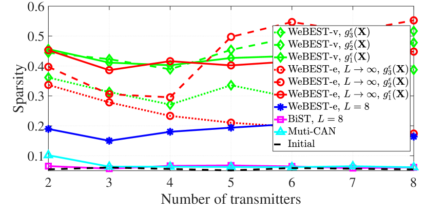
(c) Sparsity versus transmitter ($N=64$).

Figure 4: The Sparsity behavior and comparing the performance of the proposed method with other methods.

IV-E The impact of $p$

Here we evaluate the impact of $p$ on the auto- and cross-correlations. Figure 4 shows the auto-correlation of the first sequence with three different values of $p$ namely, $p\to 0$, $p=2$ and $p\to\infty$ for entry and vector optimization procedures under discrete phase constraint. As can be seen in all the cases when $p\to 0$, the auto-correlation function has many lags which are below the sparsity threshold. When $p=2$, the proposed method offers a waveform with good ISL property. By increasing the $p\to\infty$ the lags become flat and the algorithm offers a waveform with good PSL property.

(a) Discrete phase ($L=16$).

(b) Entry optimization.

(c) Vector optimization.

Figure 5: The impact of choosing $p$ on auto-correlation ($M=2$ and $N=128$).

IV-F The impact of weighting ($\mathbf{w}$)

In this part we evaluate the impact of weighting on the auto- and cross-correlation of the proposed method. Let $\mathcal{V}$ and $\mathcal{U}$ be the desired and undesired lags for MIMO radar, respectively. These two sets satisfy $\mathcal{V}\cup\mathcal{U}=\{-N+1,\dots,N-1\}$ and $\mathcal{V}\cap\mathcal{U}=\emptyset$. We assume that,

$$\begin{dcases}w_{k}=1,&k\in\mathcal{V}\\ w_{k}=0,&k\in\mathcal{U}\end{dcases}$$

Figure 6 shows the impact of weighting with $M=2$, $N=256$ and different values of $p$, under continuous phase and entry-based optimization. In addition, we assume different region of desired lags, namely, $\mathcal{V}=[-90,90]$, $\mathcal{V}=[-64,64]$ and $\mathcal{V}=[-38,38]$. As can be seen, by decreasing the range we obtain a deeper null and vice versa in all cases. Besides, in Figure 6(a), Figure 6(c) and Figure 6(b) we obtain sparse, good PSL and good ISL of auto-correlation in desired regions of lags.

(a) $p\to 0$.

(b) $p=2$.

(c) $p\to\infty$.

Figure 6: The impact of weighting in WeBEST-e with different values of $p$ ($L\to\infty$, $M=2$ and $N=256$).

In Figure 7, we compare the performance of the proposed method with MM-WeCorr and Multi-WeCAN reported in [24] and [21] respectively. In this figure we assume that $p=2$, $M=2$ and $N=512$ and we consider to put nulls within range $\mathcal{V}=[-51,51]$. As can be see, the proposed method outperforms the Multi-WeCAN method even by comparing the designed sequences with limited alphabet size. The vector optimization approach has similar performance comparing to MM-WeCorr. However, the entry optimization approach offers lower sidelobes in the lag region $\mathcal{V}=[-51,51]$ when compared to MM-WeCorr.

(a) The Auto-Correlation of the first waveform.

(b) The Cross-Correlation of the first and second waveforms.

(c) The Auto-Correlation of the second waveform.

Figure 7: Comparison of the performance of the weighted ISL minimization of the proposed method with MM-WeCorr and Multi-WECAN unde discrete phase, entry and vector optimization ($p=2$, $M=2$ and $N=512$).

IV-G Computational Time

In this subsection, we assess the computational time of WeBEST and compare it with Multi-WeCAN and MM-WeCorr. In this regard, we report the computational time by a desktop PC with Intel (R) Core (TM) i9-9900K CPU @ 3.60GHz with installed memory (RAM) 64.00 GB. Figure 8 shows the computational time of WeBEST, Multi-WeCAN and MM-WeCorr with $M=2$, $l=64$ and different sequence length. In this figure we assume that the desired lags are located at $\mathcal{V}=[-\lfloor 0.1N\rceil,\lfloor 0.1N\rceil]$. For fair comparison, we assume $\Delta\mbox{\boldmath{$X$}}=10^{-3}$ as stopping criteria for all methods. Since in WeBEST-v, we optimize a vector in each step, it is faster compare to other methods, especially with long sequence length. However, due to efficient formulation for entry-based optimization, WeBEST-e has lower computational time when compare to Multi-WeCAN and MM-WeCorr.

Figure 8: Comparison of the computational time of WeBEST with other methods. ($M=2$ and $L=64$)

V Conclusion

In this paper, we considered the $\ell_{p}$-norm of auto- and cross-correlation functions of a set of sequences as the objective function and optimized the sequences under unimodular constraint using BSUM framework. This problem formulation, provided further the flexibility for selecting $p$ and adapting waveforms based on the environmental conditions, a key requirement for the emerging cognitive radar systems. To tackle the problem, in every iterations of BSUM algorithm, we utilized a local approximation function to minimize the objective function. Specifically we introduced entry- and vector-based solutions where in the former we obtain critical points and in the latter we obtain the gradient to find the optimized solution. We further used FFT-based method for designing discrete phase sequences. Simulation results have illustrated the monotonicity of the proposed framework in minimizing the objective function. Besides, the proposed framework meets the lower bound in case of ISL minimization, and outperform the counterparts in terms of PSL, $l_{0}$-norm and computational time.

Appendix A

The auto- and cross-correlation of $t^{th}$ transmitter can be written as $d^{th}$ entry as, [27],

$$r_{t,t}(k)\triangleq\bar{c}_{ttdk}+\bar{a}_{ttdk}x_{t,d}+\bar{b}_{ttdk}x_{t,d}^{*}$$ (40)

$$r_{t,l}(k)\triangleq\bar{c}_{tldk}+\bar{a}_{tldk}x_{t,d}$$

where,

$$\bar{c}_{tldk} \triangleq\textstyle\sum_{\begin{subarray}{c}{n=1}\\ {n\neq d}\end{subarray}}^{N-k}x_{t,n}x_{l,n+k}^{*},\bar{a}_{tldk}\triangleq x_{l,d+k}^{*}I_{A}(d+k)$$ (41)

$$\bar{c}_{ttdk} \triangleq\textstyle\sum_{\begin{subarray}{c}{n=1}\\ {n\neq d,n\neq d-k}\end{subarray}}^{N-k}x_{t,n}x_{t,n+k}^{*}$$

$$\bar{a}_{ttdk} \triangleq x_{t,d+k}^{*}I_{A}(d+k),\bar{b}_{ttdk}\triangleq x_{t,d-k}I_{A}(d-k)$$

where, $I_{A}(p)$ is the indicator function of set $A=\left\{1,\dots,N\right\}$, i.e, $I_{A}(p)\triangleq\begin{dcases}1,&p\in A\\ 0,&p\notin A\end{dcases}$. Please note that the coefficients $c_{tldk}$ and $c_{ttdk}$ are depend on $\mathbf{x}_{t,-d}$ while $a_{tldk}$, $a_{ttdk}$ and $b_{ttdk}$ are depend on $x_{t,d}$.

Therefore the weighted auto- and cross-correlation of $t^{th}$ transmitter becomes,

$$w_{k}r_{t,t}(k)=c_{ttdk}+a_{ttdk}x_{t,d}+b_{ttdk}x_{t,d}^{*}$$ (42)

$$w_{k}r_{t,l}(k)=c_{tldk}+a_{tldk}x_{t,d}$$

where

$$a_{ttdk} \triangleq w_{k}\bar{a}_{ttdk},\ b_{ttdk}\triangleq w_{k}\bar{b}_{ttdk},\ c_{ttdk}\triangleq w_{k}\bar{c}_{ttdk},$$ (43)

$$a_{tldk} \triangleq w_{k}\bar{a}_{tldk},\ c_{tldk}\triangleq w_{k}\bar{c}_{tldk},$$

Substituting (42) in TABLE III, the auto- and cross- terms of $f(\mbox{\boldmath{$X$}})$, $v_{h}^{\epsilon}(\mbox{\boldmath{$X$}})$ and $u(\mbox{\boldmath{$X$}})$ with respect to $x_{t,d}$ can be written as TABLE IV.

Appendix B

By substituting $x_{t,d}=e^{j\phi}$ in $v_{au,h}^{\epsilon}(\mathbf{x}_{t})$ and $v_{cr,h}^{\epsilon}(\mathbf{x}_{t})$ in TABLE IV, they can be expressed with respect to variable $\phi$. By expanding the absolute term and separating the $e^{jn\phi}$ terms by some mathematical manipulations, the auto- and cross-correlation term of $v_{h}^{\epsilon}(\phi)$ can be written as,

$$v_{h,au}^{\epsilon}(\phi)=\textstyle\sum_{n=-2}^{2}\bar{v}_{h,n}e^{jn\phi},\ v_{h,cr}^{\epsilon}(\phi)=\sum_{n=-1}^{1}\tilde{v}_{h,n}e^{jn\phi},$$ (44)

where,

$$\bar{v}_{h,-2}\triangleq\textstyle\sum_{k=-N+1}^{N-1}\gamma_{httk}(a_{ttdk}^{*}b_{ttdk}),\quad\bar{v}_{h,2}\triangleq\bar{v}_{h,-2}^{*},$$

$$\bar{v}_{h,-1}\triangleq\textstyle\sum_{k=-N+1}^{N-1}\gamma_{httk}(a_{ttdk}^{*}c_{ttdk}+c_{ttdk}^{*}b_{ttdk}),\ \bar{v}_{h,1}\triangleq\bar{v}_{h,-1}^{*},$$

$$\bar{v}_{h,0}\triangleq\textstyle\sum_{k=-N+1}^{N-1}(\gamma_{httk}(|c_{ttdk}|^{2}+|a_{ttdk}|^{2}+|b_{ttdk}|^{2})+\mu_{httk}).$$

$$\tilde{v}_{h,-1}\triangleq\textstyle 2\sum_{\begin{subarray}{c}{l=1}\\ {l\neq t}\end{subarray}}^{M}\sum_{k=-N+1}^{N-1}\gamma_{htlk}a_{tldk}^{*}c_{tldk},\quad\tilde{v}_{h,1}\triangleq\tilde{v}_{h,-1}^{*},$$

$$\tilde{v}_{h,0}\triangleq\textstyle 2\sum_{\begin{subarray}{c}{l=1}\\ {l\neq t}\end{subarray}}^{M}\sum_{k=-N+1}^{N-1}(\gamma_{htlk}(|c_{tldk}|^{2}+|a_{tldk}|^{2})+\mu_{htlk}).$$

Since, $v_{h}^{\epsilon}(\phi)=v_{h,au}^{\epsilon}(\phi)+v_{h,cr}^{\epsilon}(\phi)+v_{h,m}^{\epsilon}$, it can be written as (18), where,

$$v_{h,-2}\triangleq\bar{v}_{h,-2},\ v_{h,-1}\triangleq\bar{v}_{h,-1}+\tilde{v}_{h,-1}$$ (45)

$$v_{h,0}\triangleq\bar{v}_{h,0}+\tilde{v}_{h,0}+v_{h,m}^{\epsilon},\ v_{h,1}\triangleq\bar{v}_{h,-1}^{*}\ v_{h,2}\triangleq\bar{v}_{h,-2}^{*}$$

Like wise, by substituting $x_{t,d}=e^{j\phi}$ in $u_{au}(\mathbf{x}_{t})$ and $u_{cr}(\mathbf{x}_{t})$, they can be expressed with respect to variable $\phi$. Let, $\phi^{(i)}=\angle{x_{t,d}^{(i)}}$, hence, $w_{k}r_{t,l}^{(i)}(k)=c_{tldk}+a_{tldk}e^{j\phi^{(i)}}$ and $w_{k}r_{t,t}^{(i)}(k)=c_{ttdk}+a_{ttdk}e^{j\phi^{(i)}}+b_{ttdk}e^{-j\phi^{(i)}}$ respectively. Therefore $u_{au}(\phi)$ and $u_{cr}(\phi)$ becomes,

$$u_{au}(\phi)=\textstyle\sum_{n=-2}^{2}\bar{u}_{n}e^{jn\phi}+\Re\left\{\sum_{n=-1}^{1}\hat{u}_{n}e^{jn\phi}\right\},$$

$$u_{cr}(\phi)=\textstyle\sum_{n=-1}^{1}\tilde{u}_{n}e^{jn\phi}+\Re\left\{\sum_{n=-1}^{0}\check{u}_{n}e^{jn\phi}\right\},$$

Defining $\psi_{ttdk}^{\prime}\triangleq\frac{\psi_{ttdk}}{|w_{k}r_{t,t}^{(i)}(k)|}$ and $\psi_{tldk}^{\prime}\triangleq\frac{\psi_{tldk}}{|w_{k}r_{t,l}^{(i)}(k)|}$, it can be shown that,

$$\bar{u}_{-2}\triangleq\textstyle\sum_{k=-N+1}^{N-1}\eta_{ttdk}a_{ttdk}^{*}b_{ttdk},\quad\bar{u}_{2}\triangleq\bar{u}_{-2}^{*},$$

$$\bar{u}_{-1}\triangleq\textstyle\sum_{k=-N+1}^{N-1}\eta_{ttdk}(a_{ttdk}^{*}c_{ttdk}+c_{ttdk}^{*}b_{ttdk}),\quad\bar{u}_{1}\triangleq\bar{u}_{-1}^{*},$$

$$\bar{u}_{0}\triangleq\textstyle\sum_{k=-N+1}^{N-1}(\eta_{ttdk}(|c_{ttdk}|^{2}+|a_{ttdk}|^{2}+|b_{ttdk}|^{2})+\nu_{ttdk})$$

$$\hat{u}_{-1}\textstyle\triangleq\sum_{k=-N+1}^{N-1}\psi_{ttdk}^{\prime}(|c_{ttdk}|^{2}+c_{ttdk}^{*}a_{ttdk}e^{j\phi^{(i)}}+c_{ttdk}^{*}b_{ttdk}e^{-j\phi^{(i)}})$$

$$\hat{u}_{0}\triangleq\textstyle\sum_{k=-N+1}^{N-1}\psi_{ttdk}^{\prime}(|b_{ttdk}|^{2}e^{-j\phi^{(i)}}+b_{ttdk}^{*}a_{ttdk}e^{j\phi^{(i)}}+b_{ttdk}^{*}c_{ttdk})$$

$$\hat{u}_{1}\triangleq\textstyle\sum_{k=-N+1}^{N-1}\psi_{ttdk}^{\prime}(|a_{ttdk}|^{2}e^{j\phi^{(i)}}+a_{ttdk}^{*}b_{ttdk}e^{-j\phi^{(i)}}+a_{ttdk}^{*}c_{ttdk})$$

$$\tilde{u}_{-1}\triangleq\textstyle 2\sum_{\begin{subarray}{c}{l=1}\\ {l\neq t}\end{subarray}}^{M}\sum_{k=-N+1}^{N-1}\eta_{tldk}c_{tldk}a_{tldk}^{*},\quad\tilde{u}_{1}\triangleq\tilde{u}_{-1}^{*}$$

$$\tilde{u}_{0}\triangleq\textstyle 2\sum_{\begin{subarray}{c}{l=1}\\ {l\neq t}\end{subarray}}^{M}\sum_{k=-N+1}^{N-1}(\eta_{tldk}(|c_{tldk}|^{2}+|a_{tldk}|^{2})+\nu_{tldk}))$$

$$\check{u}_{-1}\triangleq\textstyle 2\sum_{\begin{subarray}{c}{l=1}\\ {l\neq t}\end{subarray}}^{M}\sum_{k=-N+1}^{N-1}\psi_{tldk}^{\prime}(c_{tldk}a_{tldk}^{*}+|a_{tldk}|^{2}e^{j\phi^{(i)}})$$

$$\check{u}_{0}\triangleq\textstyle 2\sum_{\begin{subarray}{c}{l=1}\\ {l\neq t}\end{subarray}}^{M}\sum_{k=-N+1}^{N-1}\psi_{tldk}^{\prime}(|c_{tldk}|^{2}+c_{tldk}^{*}a_{tldk}e^{j\phi^{(i)}})$$

Since $u(\phi)$ is a real function, it can be written as $u(\phi)=\Re\left\{u_{au}(\phi)+u_{cr}(\phi)+u_{m}\right\}$, specifically can be written as (18), where,

$$u_{-2}\triangleq\bar{u}_{-2},\quad u_{-1}\triangleq\tilde{u}_{-1}+\bar{u}_{-1}+\hat{u}_{-1}+\check{u}_{-1}$$

$$u_{0}\triangleq\bar{u}_{0}+\hat{u}_{0}+\tilde{u}_{0}+\check{u}_{0}+u_{m},\ u_{1}=\tilde{u}_{1}+\bar{u}_{1}+\hat{u}_{1},\ u_{2}\triangleq\bar{u}_{2}$$

Appendix C

Substituting $e^{jn\phi}=\cos{(n\phi)}+j\sin{(n\phi)}$ in $u^{\prime}(\phi)$ and separating the real and imaginary part, $u^{\prime}(\phi)$ becomes,

$$u^{\prime}(\phi) =\xi_{0}\cos^{2}(\phi)+\xi_{1}\sin^{2}(\phi)+\xi_{2}\sin(\phi)\cos(\phi)$$ (46)

$$+\xi_{3}\cos(\phi)+\xi_{4}\sin(\phi)$$

where, $\xi_{0}\triangleq 2\Im\{u_{-2}-u_{2}\}$, $\xi_{1}\triangleq 2\Im\{u_{2}-u_{-2}\}$, $\xi_{2}\triangleq-4\Re\{u_{2}+u_{-2}$}, $\xi_{3}\triangleq\Im\{u_{-1}-u_{1}\}$ and $\xi_{4}\triangleq-\Re\{u_{-1}+u_{1}\}$. Using the change variable $z\triangleq\tan(\frac{\phi}{2})$ and substituting $\cos(\phi)={(1-z^{2})}/{(1+z^{2})}$, $\sin(\phi)={2z}/{(1+z^{2})}$ in $u^{\prime}(\phi)$, it can be written as, $u^{\prime}(z)=\frac{\sum_{k=0}^{4}s_{k}z^{k}}{(1+z^{2})^{2}}$, where,

$$s_{0}\triangleq\xi_{0}+\xi_{3},\ s_{1}\triangleq 2(\xi_{2}+\xi_{4}),\ s_{2}\triangleq 2(2\xi_{1}-\xi_{0}),$$ (47)

$$s_{3}\triangleq 2(\xi_{4}-\xi_{2}),\ s_{4}\triangleq\xi_{0}-\xi_{3}$$

Likewise, considering $z\triangleq\tan(\frac{\phi}{2})$, the roots of $v_{h}^{\epsilon^{\prime}}(\phi)$ can be equivalently obtained by solving $\frac{\sum_{k=0}^{4}q_{h,k}z^{k}}{(1+z^{2})^{2}}=0$, where,

$$q_{h,0}\triangleq\varkappa_{0}+\varkappa_{3},\ q_{h,1}\triangleq 2(\varkappa_{2}+\varkappa_{4}),\ q_{h,2}\triangleq 2(2\varkappa_{1}-\varkappa_{0}),$$ (48)

$$q_{h,3}\triangleq 2(\varkappa_{4}-\varkappa_{2}),\ q_{h,4}\triangleq\varkappa_{0}-\varkappa_{3},$$

and, $\varkappa_{0}\triangleq-4\Im\{v_{h,2}\}$, $\varkappa_{1}\triangleq 4\Im\{v_{h,2}\}$, $\varkappa_{2}\triangleq-8\Re\{v_{h,2}\}$, $\varkappa_{3}\triangleq-2\Im\{v_{h,1}\}$ and $\varkappa_{4}\triangleq-2\Re\{v_{h,1}\}$.

Appendix D

Under discrete phase constraint, since the phases are chosen from finite alphabet ($\phi\in\Omega_{L}$) the objective function can be written with respect to the the indices of $\Omega_{L}$ as follows,

$$f(l^{\prime})=f(\mbox{\boldmath{$X$}}_{-t})+\textstyle 2\sum_{\begin{subarray}{c}{l=1}\\ {l\neq t}\end{subarray}}^{M}\sum_{k=-N+1}^{N-1}|a_{tldk}+c_{tldk}e^{-j2\pi\frac{l^{\prime}-1}{L}}|^{p}$$ (49)

$$+\sum_{k=-N+1}^{N-1}|a_{ttdk}+c_{ttdk}e^{-j2\pi\frac{l^{\prime}-1}{L}}+b_{ttdk}e^{-j4\pi\frac{l^{\prime}-1}{L}}|^{p}$$

Observe that $a_{tldk}+c_{tldk}e^{-j2\pi\frac{l^{\prime}-1}{L}}$ and $a_{ttdk}+c_{ttdk}e^{-j2\pi\frac{l^{\prime}-1}{L}}+b_{ttdk}e^{-j4\pi\frac{l^{\prime}-1}{L}}$ exactly follow the definition of $L$-points DFT of sequences $\{a_{tldk},c_{tldk}\}$ and $\{a_{ttdk},c_{ttdk},b_{ttdk}\}$ respectively. Therefore, $f(l^{\prime})$ can be written as (23).

References

• [1] S. D. Blunt and E. L. Mokole, “Overview of radar waveform diversity,” IEEE Aerospace and Electronic Systems Magazine, vol. 31, no. 11, pp. 2–42, 2016.
• [2] M. Kumar and V. Chandrasekar, “Intrapulse polyphase coding system for second trip suppression in a weather radar,” IEEE Transactions on Geoscience and Remote Sensing, vol. 58, no. 6, pp. 3841–3853, 2020.
• [3] J. M. Baden, “Efficient optimization of the merit factor of long binary sequences,” IEEE Trans. Inf. Theory, vol. 57, no. 12, pp. 8084–8094, Dec 2011.
• [4] H. Sun, F. Brigui, and M. Lesturgie, “Analysis and comparison of MIMO radar waveforms,” in 2014 International Radar Conference, Oct 2014, pp. 1–6.
• [5] “Texas instrument: MIMO radar, application report, swra554,” https://www.ti.com/lit/an/swra554a/swra554a.pdf, accessed: 2021-03-15.
• [6] C. Hammes, B. S. M. R., and B. Ottersten, “Generalized multiplexed waveform design framework for cost-optimized mimo radar,” IEEE Trans. Signal Process., vol. 69, pp. 88–102, 2021.
• [7] “Ultra-small, economical and cheap radar made possible thanks to chip technology,” https://www.imec-int.com/en/imec-magazine/imec-magazine-march-2018/ultra-small-economical-and-cheap-radar-made-possible-thanks-to-chip-technology, accessed: 2021-03-15.
• [8] J. R. Guerci, R. M. Guerci, M. Ranagaswamy, J. S. Bergin, and M. C. Wicks, “CoFAR: Cognitive fully adaptive radar,” in 2014 IEEE Radar Conference, 2014, pp. 0984–0989.
• [9] P. Stinco, M. Greco, F. Gini, and B. Himed, “Cognitive radars in spectrally dense environments,” IEEE Aerospace and Electronic Systems Magazine, vol. 31, no. 10, pp. 20–27, 2016.
• [10] S. Z. Gurbuz, H. D. Griffiths, A. Charlish, M. Rangaswamy, M. S. Greco, and K. Bell, “An overview of cognitive radar: Past, present, and future,” IEEE Aerospace and Electronic Systems Magazine, vol. 34, no. 12, pp. 6–18, 2019.
• [11] A. De Maio and A. Farina, “The role of cognition in radar sensing,” in 2020 IEEE Radar Conference (RadarConf20), 2020, pp. 1–6.
• [12] P. Stoica, H. He, and J. Li, “New algorithms for designing unimodular sequences with good correlation properties,” IEEE Trans. Signal Process., vol. 57, no. 4, pp. 1415–1425, Apr 2009.
• [13] P. Stoica, H. He, and J. Li, “On designing sequences with impulse-like periodic correlation,” IEEE Signal Processing Letters, vol. 16, no. 8, pp. 703–706, 2009.
• [14] J. Song, P. Babu, and D. Palomar, “Optimization methods for designing sequences with low autocorrelation sidelobes,” IEEE Trans. Signal Process., vol. 63, no. 15, pp. 3998–4009, Aug 2015.
• [15] J. Song, P. Babu, and D. P. Palomar, “Sequence design to minimize the weighted integrated and peak sidelobe levels,” IEEE Trans. Signal Process., vol. 64, no. 8, pp. 2051–2064, Apr 2016.
• [16] L. Zhao, J. Song, P. Babu, and D. P. Palomar, “A unified framework for low autocorrelation sequence design via Majorization-Minimization,” IEEE Trans. Signal Process., vol. 65, no. 2, pp. 438–453, Jan 2017.
• [17] J. Liang, H. C. So, J. Li, and A. Farina, “Unimodular sequence design based on alternating direction method of multipliers,” IEEE Trans. Signal Process., vol. 64, no. 20, pp. 5367–5381, 2016.
• [18] M. Alaee-Kerahroodi, A. Aubry, A. De Maio, M. M. Naghsh, and M. Modarres-Hashemi, “A coordinate-descent framework to design low PSL/ISL sequences,” IEEE Trans. Signal Process., vol. 65, no. 22, pp. 5942–5956, Nov 2017.
• [19] J. M. Baden, B. O’Donnell, and L. Schmieder, “Multiobjective sequence design via gradient descent methods,” IEEE Trans. Aerosp. Electron. Syst., vol. 54, no. 3, pp. 1237–1252, June 2018.
• [20] R. Lin, M. Soltanalian, B. Tang, and J. Li, “Efficient design of binary sequences with low autocorrelation sidelobes,” IEEE Trans. Signal Process., vol. 67, no. 24, pp. 6397–6410, Dec 2019.
• [21] H. He, P. Stoica, and J. Li, “Designing unimodular sequence sets with good correlations; including an application to MIMO radar,” IEEE Trans. Signal Process., vol. 57, no. 11, pp. 4391–4405, Nov 2009.
• [22] G. Cui, X. Yu, M. Piezzo, and L. Kong, “Constant modulus sequence set design with good correlation properties,” Signal Processing, vol. 139, pp. 75–85, 2017.
• [23] Y. Li and S. A. Vorobyov, “Fast algorithms for designing unimodular waveform(s) with good correlation properties,” IEEE Trans. Signal Process., vol. 66, no. 5, pp. 1197–1212, March 2018.
• [24] J. Song, P. Babu, and D. P. Palomar, “Sequence set design with good correlation properties via majorization-minimization,” IEEE Trans. Signal Process., vol. 64, no. 11, pp. 2866–2879, June 2016.
• [25] M. Alaee-Kerahroodi, M. R. Bhavani Shankar, K. V. Mishra, and B. Ottersten, “Meeting the lower bound on designing set of unimodular sequences with small aperiodic/periodic isl,” in 2019 20th International Radar Symposium (IRS), 2019, pp. 1–13.
• [26] E. Raei, M. Alaee-Kerahrood, and M. R. B. Shankar, “Spatial- and range- ISLR trade-off in MIMO radar via waveform correlation optimization,” 2021.
• [27] M. Alaee-Kerahroodi, M. Modarres-Hashemi, and M. M. Naghsh, “Designing sets of binary sequences for MIMO radar systems,” IEEE Trans. Signal Process., pp. 1–1, 2019.
• [28] S. P. Sankuru, R. Jyothi, P. Babu, and M. Alaee-Kerahroodi, “Designing sequence set with minimal peak side-lobe level for applications in high resolution radar imaging,” IEEE Open Journal of Signal Processing, vol. 2, pp. 17–32, 2021.
• [29] F. Laforest, “Generic models: a new approach for information systems design,” in Proceedings of the Third Basque International Workshop on Information Technology - BIWIT’97 - Data Management Systems, 1997, pp. 189–196.
• [30] M. Hong, M. Razaviyayn, Z. Luo, and J. Pang, “A unified algorithmic framework for block-structured optimization involving big data: With applications in machine learning and signal processing,” IEEE Signal Processing Magazine, vol. 33, no. 1, pp. 57–77, 2016.
• [31] P. Borwein and R. Ferguson, “Polyphase sequences with low autocorrelation,” IEEE Trans. Inf. Theory, vol. 51, no. 4, pp. 1564–1567, Apr 2005.
• [32] W. Huang, M. M. Naghsh, R. Lin, and J. Li, “Doppler sensitive discrete-phase sequence set design for MIMOs radar,” IEEE Trans. Aerosp. Electron. Syst., pp. 1–1, 2020.
• [33] L. Zhao and D. P. Palomar, “Maximin joint optimization of transmitting code and receiving filter in radar and communications,” IEEE Trans. Signal Process., vol. 65, no. 4, pp. 850–863, Feb 2017.
• [34] J. Song, P. Babu, and D. P. Palomar, “Sparse generalized eigenvalue problem via smooth optimization,” IEEE Trans. Signal Process., vol. 63, no. 7, pp. 1627–1642, 2015.
• [35] S. Boyd and L. Vandenberghe, Convex optimization.   Cambridge university press, 2004.
• [36] M. R. B. Shankar and K. V. S. Hari, “Reduced complexity equalization schemes for zero padded ofdm systems,” IEEE Signal Processing Letters, vol. 11, no. 9, pp. 752–755, 2004.
• [37] G. H. Golub and C. F. Van Loan, Matrix Computations, 3rd ed.   The Johns Hopkins University Press, 1996.
• [38] H. He, J. Li, and P. Stoica, Waveform Design for Active Sensing Systems.   Cambridge University Press, 2012.
• [39] K. Mohammad, Alaee, A. Augusto, N. Mohammad, Mahdi, M. Antonio, De, and H. Mahmoud, Modarres, Radar Waveform Design Based on Optimization Theory.   Institution of Engineering and Technology, 2020, ch. A computational design of phase-only (possibly binary) sequences for radar systems, pp. 63–92.