Muon and electron g-2 and proton and cesium weak charges implications on dark $\mathbf{Z_{d}}$ models

Abstract

Theories beyond the standard model involving a sub-GeV-scale vector $Z_{d}$ mediator have been largely studied as a possible explanation of the experimental values of the muon and electron anomalous magnetic moments. Motivated by the recent determination of the anomalous muon magnetic moment performed at Fermilab, we derive the constraints on such a model obtained from the magnetic moment determinations and the measurements of the proton and cesium weak charge, $Q_{W}$, performed at low-energy transfer. In order to do so, we revisit the determination of the cesium $Q_{W}$ from the atomic parity violation experiment, which depends critically on the value of the average neutron rms radius of ${}^{133}\text{Cs}$, by determining the latter from a practically model-independent extrapolation from the recent average neutron rms radius of ${}^{208}\text{Pb}$ performed by the PREX-2 Collaboration. From a combined fit of all the aforementioned experimental results, we obtain rather precise limits on the mass and the kinetic mixing parameter of the $Z_{d}$ boson, namely $m_{Z_{d}}=47{}^{+61}_{-16}\,\mathrm{MeV}$ and $\varepsilon=2.3{}^{+1.1}_{-0.4}\times 10^{-3}$, when marginalizing over the $Z-Z_{d}$ mass mixing parameter $\delta$.

A new measurement of the anomalous muon magnetic moment, referred to as $a_{\mu}\equiv(g_{\mu}-2)/2$, has been largely awaited due to the presence of a long-standing deviation of the experimental determination of $a_{\mu}$, performed at BNL Bennett et al. (2006) in 2004, from the theoretical expectation of about $3.7\sigma$. Recently, the Muon g-2 Collaboration at Fermilab (FNAL) released a new measurement Abi et al. (2021), with a slightly better precision, about $15\%$ less, than the BNL one, which is $a_{\mu}^{\rm FNAL,\,exp}=116\ 592\ 040(54)\times 10^{-11}$. The combined experimental average between the FNAL and BNL results

$$a_{\mu}^{\rm exp}=116\ 592\ 061(41)\times 10^{-11},$$ (1)

can be compared with the standard model (SM) prediction $a_{\mu}^{\rm SM}=116\ 591\ 810(43)\times 10^{-11}$ Aoyama et al. (2020, 2012, 2019); Czarnecki et al. (2003); Gnendiger et al. (2013); Davier et al. (2017); Keshavarzi et al. (2018); Colangelo et al. (2019); Hoferichter et al. (2019); Davier et al. (2020); Keshavarzi et al. (2020); Melnikov and Vainshtein (2004); Masjuan and Sánchez-Puertas (2017); Colangelo et al. (2017); Hoferichter et al. (2018); Gérardin et al. (2019); Bijnens et al. (2019); Colangelo et al. (2020); Pauk and Vanderhaeghen (2014); Danilkin and Vanderhaeghen (2017); Jegerlehner (2017); Knecht et al. (2018); Eichmann et al. (2020); Roig and Sánchez-Puertas (2020); Blum et al. (2020); Colangelo et al. (2014), showing an intriguing $4.2\sigma$ discrepancy

$$\Delta a_{\mu}=a_{\mu}^{\rm exp}-a_{\mu}^{\rm SM}=251(59)\times 10^{-11}.$$ (2)

This breakthrough result strengthens the motivation for the development of SM extensions, in particular in light of other increasing evidences for the incompleteness of the SM recently reported Aaij et al. (2021).

In the last years, also the electron anomalous magnetic moment experimental result Hanneke et al. (2008, 2011) has shown a greater than $2\sigma$ discrepancy with the SM prediction Parker et al. (2018), even if with an opposite sign with respect to the muon one. However, a new determination of the fine structure constant Morel et al. (2020), obtained from the measurement of the recoil velocity on rubidium atoms, resulted into a reevaluation of the SM electron magnetic moment, bringing to a positive discrepancy of about $1.6\sigma$. Namely

$$\Delta a_{e}=a_{e}^{\rm exp}-a_{e}^{\rm SM,\,Rb}=0.48(30)\times 10^{-12},$$ (3)

where $a_{e}\equiv(g_{e}-2)/2$. Interestingly, now the electron and muon magnetic moment discrepancies point to the same direction.

These longstanding anomalies have motivated a variety of theoretical models that predict the existence of yet to be discovered particles that might contribute to the process Fayet (2007); Davoudiasl and Marciano (2018); Cadeddu et al. (2021a); Bœhm and Fayet (2004); Giudice et al. (2012); Bodas et al. (2021). In particular, they could indicate the presence of an additional sub-GeV-scale gauge boson, referred to as $Z_{d}$ Davoudiasl et al. (2012a, b, 2013); Arcadi et al. (2019). Here, we recall the basic features of such a model in which we assume a $U(1)_{d}$ gauge symmetry associated with a hidden dark sector. The corresponding $Z_{d}$ gauge boson couples to the SM bosons via kinetic mixing, parametrized by $\varepsilon$, and $Z$-$Z_{d}$ mass matrix mixing, parametrized by $\varepsilon_{Z}=(m_{Z_{d}}/m_{Z})\delta$ Davoudiasl et al. (2012a), where $m_{Z_{d}}$ and $m_{Z}$ are the $Z_{d}$ and $Z$ masses, respectively. The parameter $\delta$ in the latter relation is usually replaced Davoudiasl et al. (2015) by the following expression

$$\delta^{\prime}\simeq\delta+\frac{m_{Z_{d}}}{m_{Z}}\,\varepsilon\,\tan\theta_{W},$$ (4)

that incorporates higher order corrections, even if small for $m_{Z_{d}}\ll m_{Z}$. Here, $\theta_{W}$ is the SM predicted running of the Weinberg angle in the modified minimal subtraction ($\overline{\mathrm{MS}}$) renormalization scheme Zyla et al. (2020); Erler and Ramsey-Musolf (2005); Erler and Ferro-Hernández (2018).

As a consequence of the mixing, the $Z_{d}$ coupling with the SM results into an interaction Lagrangian Davoudiasl et al. (2012a, b, 2013)

$${\cal L}_{\text{int}}=(-e\varepsilon J^{em}_{\mu}-\frac{g}{2\cos\theta_{W}}\frac{m_{Z_{d}}}{m_{Z}}\delta^{\prime}J^{NC}_{\mu})Z_{d}^{\mu},$$ (5)

where $e$ is the electric charge, $J_{\mu}^{NC}$ and $J_{\mu}^{em}$ are respectively the neutral and electromagnetic currents, whereas $Z_{d}^{\mu}$ is the new boson field.
Within this model, the new weak neutral current amplitudes at low $Q^{2}$ momentum transfer can be retrieved through the substitutions $G_{F}\to\rho_{d}G_{F}$, $G_{F}$ being the Fermi coupling constant, and $\sin^{2}\theta_{W}(Q^{2})\to\kappa_{d}\,\sin^{2}\theta_{W}(Q^{2})$ Davoudiasl et al. (2012a, 2015, c, 2014), where

$$\rho_{d} =1+(\delta+\frac{m_{Z_{d}}}{m_{Z}}\,\varepsilon\,\tan\theta_{W})^{2}f\Big{(}\frac{Q^{2}}{m_{Z_{d}}^{2}}\Big{)},$$ (6)

and

$$\kappa_{d} =1-\varepsilon(\delta+\frac{m_{Z_{d}}}{m_{Z}}\,\varepsilon\,\tan\theta_{W})\frac{m_{Z}}{m_{Z_{d}}}\cot\theta_{W}f\Big{(}\frac{Q^{2}}{m_{Z_{d}}^{2}}\Big{)}.$$ (7)

The term $f({Q^{2}}/{m_{Z_{d}}^{2}})$ is related to the propagator of the new boson and it may assume different forms depending on the experimental process Bouchiat and Piketty (1983); Bouchiat and Fayet (2005).

The one-loop vector contribution to the magnetic moment of the lepton $l=e,\,\mu$ which arises from this model is Davoudiasl et al. (2012d)

$$a_{l,\,\text{vector}}^{Z_{d}}=\frac{\alpha}{2\pi}\Big{(}\varepsilon+\frac{m_{Z_{d}}}{m_{Z}}\delta^{\prime}\frac{1-4\sin^{2}\theta_{W}}{4\sin\theta_{W}\cos\theta_{W}}\Big{)}^{2}F_{V}\Big{(}\frac{m_{Z_{d}}}{m_{l}}\Big{)},$$ (8)

where $\sin\theta_{W}$ is employed at the corresponding lepton mass scale, $\alpha$ is the fine-structure constant, $m_{l}$ the lepton mass and

$$F_{V}(x)\equiv\int_{0}^{1}dz\frac{2z(1-z)^{2}}{(1-z)^{2}+x^{2}z}.$$ (9)

The mass mixing introduces also an axial contribution, which is although negligible, given by Davoudiasl et al. (2012d)

$$a_{l,\,\text{axial}}^{Z_{d}}=-\frac{G_{F}m_{l}^{2}}{8\sqrt{2}\pi^{2}}\delta^{\prime 2}F_{A}\Big{(}\frac{m_{Z_{d}}}{m_{l}}\Big{)},$$ (10)

where

$$F_{A}(x)\equiv\int_{0}^{1}dz\frac{2(1-z)^{3}+x^{2}z(1-z)(z+3)}{(1-z)^{2}+x^{2}z}.$$ (11)

Adding the two contributions in Eqs. (8) and (10), it is possible to retrieve the total $Z_{d}$ induced magnetic momentum contribution $a_{l}^{Z_{d}}(\varepsilon,\,\delta,\,m_{Z_{d}})=a_{l,\,\text{vector}}^{Z_{d}}+a_{l,\,\text{axial}}^{Z_{d}}.$

Another consequence of the existence of this additional $Z_{d}$ boson, besides the modification of the lepton magnetic moment, would be the introduction of a new source of parity violation that could be tested by experiments sensitive to the weak charge, $Q_{W}$, of both protons and nuclei. In particular, recently the ${\rm Q_{weak}}$ Collaboration at JLAB Androic et al. (2018) measured the proton weak charge at $Q^{2}=0.0248\,\mathrm{GeV^{2}}$ to be

$$Q_{W}^{p,\,\rm exp}=0.0719(45),$$ (12)

which has to be compared with the SM prediction Erler and Su (2013); Zyla et al. (2020) that, taking into account radiative corrections, is

$$Q_{W}^{p,\,\rm SM}=-2g^{ep}_{AV}(\sin^{2}\theta_{W})\Big{(}1-\frac{\alpha}{2\pi}\Big{)}=0.0711(2),$$ (13)

where $g^{ep}_{AV}$ is the SM electron-proton coupling, which depends on the weak mixing angle at the appropriate experimental energy scale.
Similarly, in the low-energy sector, atomic parity violation (APV) experiments provide the measurement of the weak charge of a nucleus $\mathcal{N}$ with $N$ neutrons and $Z$ protons, which is also very sensitive to new vector bosons. So far, the most precise measurement has been performed at $Q\approx 2.4\ \mathrm{MeV}$ using cesium atoms ($N_{\mathrm{Cs}}=78$ and $Z_{\mathrm{Cs}}=55$), for which one can derive the following SM prediction Zyla et al. (2020) which also includes radiative corrections

$$Q_{W}^{\mathrm{{}^{133}Cs},\,\mathrm{SM}} =-2\,[\,Z_{\mathrm{Cs}}(g^{ep}_{AV}(\sin^{2}\theta_{W})+0.00005)$$

$$+N_{\mathrm{Cs}}(g^{en}_{AV}+0.00006)]\Big{(}1-\frac{\alpha}{2\pi}\Big{)}$$

$$=-73.23(1),$$ (14)

where $g^{en}_{AV}$ is the SM electron-neutron coupling. The current experimental measurement Wood et al. (1997); Guena et al. (2005); Zyla et al. (2020)

$$Q_{W}^{\mathrm{{}^{133}Cs},\,\mathrm{PDG}}=-72.82(42),$$ (15)

depends strongly on the value of the average neutron rms radius of ${}^{133}\text{Cs}$, $R_{n}(^{133}\text{Cs})$ Pollock and Welliver (1999); Pollock et al. (1992); Horowitz et al. (2001). Since at the time of Refs. Dzuba et al. (2012); Derevianko (2001) there was not any cesium neutron radius measurement, the correction on $Q_{W}^{\mathrm{{}^{133}Cs},\ \mathrm{PDG}}$ due to the difference between $R_{n}(^{133}\text{Cs})$ and $R_{p}(^{133}\text{Cs})$, the average proton rms radius, could only have been estimated exploiting hadronic probes, using an extrapolation of data from antiprotonic atom x-rays Trzcińska et al. (2001). From these data, the value of the so-called neutron skin, $\Delta R_{np}\equiv R_{n}-R_{p}$, has been measured for a number of elements, from which the extrapolated neutron skin value for each nucleus was found assuming a linear dependence on the asymmetry parameter, $I=(N-Z)/A$, where $A$ is the mass number, leading to the empirically fitted function

$$\Delta R_{np}^{\mathrm{had}}(\mathcal{N})=(-0.04\pm 0.03)+\left(1.01\pm 0.15\right)\,I\textrm{ fm}.$$ (16)

Using the latter equation, the extrapolated value of the neutron skin of ${}^{133}\text{Cs}$ is $\Delta R_{np}^{\mathrm{had}}(\mathrm{{}^{133}Cs})=0.13(4)\textrm{ fm}$, that combined with the very well known value of $R_{p}(^{133}\text{Cs})=4.807(1)\textrm{ fm}$ at the time Johnson and Soff (1985), gave a value of $R_{n}(^{133}\text{Cs})=4.94(4)\textrm{ fm}$ and a correction to $Q_{W}^{\mathrm{{}^{133}Cs},\,\mathrm{PDG}}$ explicitly visible in Table IV of Ref. Dzuba et al. (2012). However, these determinations of the neutron skin with hadronic measurements are known to be affected, unlike electroweak measurements, by considerable model dependencies and uncontrolled approximations Thiel et al. (2019). In this paper, we revisit the determination of $Q_{W}^{\mathrm{{}^{133}Cs}}$ determining $R_{n}(^{133}\text{Cs})$ from a practically model-independent extrapolation from the recent average neutron rms radius of ${}^{208}\text{Pb}$ performed by the PREX-1 and PREX-2 experiments Horowitz et al. (2012); Adhikari et al. (2021); Abrahamyan et al. (2012); Reed (2020), which exploit parity violating electron scattering on lead. Indeed, the PREX collaboration released a unique determination of the point neutron skin, the difference between the point neutron and proton rms radii $R_{p,n}^{\text{point}}$, that is equal to Horowitz et al. (2012); Adhikari et al. (2021); Abrahamyan et al. (2012); Reed (2020)

$$\Delta R_{np}^{\mathrm{point}}(^{208}\text{Pb})\equiv R_{n}^{\mathrm{point}}-R_{p}^{\rm{point}}=0.283(71)\,\mathrm{fm}.$$ (17)

We note that, this value is significantly larger with respect to the one that could be retrieved using the extrapolation in Eq. (16), corresponding to $\Delta R_{np}^{\mathrm{had}}(^{208}\text{Pb})=0.17(4)\,\mathrm{fm}$. Given that the PREX measurement is basically model independent and thus more reliable, this large discrepancy motivated us to discard the determination of $R_{n}(^{133}\text{Cs})$ from hadronic probes in favor of the usage of electroweak probes.

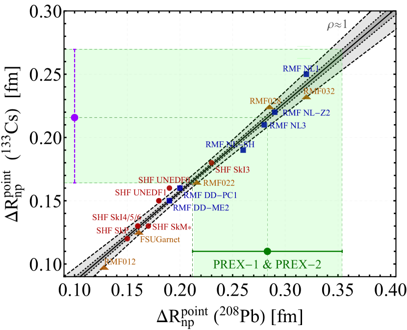
Figure 1: Point neutron skin predictions for ${}^{208}\text{Pb}$ and ${}^{133}\text{Cs}$ according to different models (red circles Dobaczewski et al. (1984); Bartel et al. (1982); Kortelainen et al. (2012, 2010); Chabanat et al. (1998); Reinhard and Flocard (1995), orange triangles Hernandez (2019); Yang et al. (2019); Chen and Piekarewicz (2014, 2015), and blue squares Sharma et al. (1993); Bender et al. (1999); Lalazissis et al. (1997); Reinhard et al. (1986); Niksic et al. (2008, 2002)). A linear fit is superimposed in solid black, where the $1\sigma$ and $3\sigma$ constraints are also shown by the dark-gray dotted and light-gray dashed regions, respectively. Constraints set by the combination of PREX-1 and PREX-2 Horowitz et al. (2012); Adhikari et al. (2021); Abrahamyan et al. (2012); Reed (2020) and the constraint on $\Delta R_{\mathrm{np}}^{\mathrm{point}}(^{133}\text{Cs})$ derived in this work are also shown by the green and purple point, respectively.

To this purpose, in Fig. 1 we show the values of the point neutron skins of ${}^{133}\text{Cs}$, and ${}^{208}\text{Pb}$ obtained with various nonrelativistic Skyrme-Hartree-Fock (SHF) Dobaczewski et al. (1984); Bartel et al. (1982); Kortelainen et al. (2012, 2010); Chabanat et al. (1998); Reinhard and Flocard (1995) and relativistic mean-field (RMF) Sharma et al. (1993); Bender et al. (1999); Lalazissis et al. (1997); Reinhard et al. (1986); Niksic et al. (2008, 2002); Hernandez (2019); Yang et al. (2019); Chen and Piekarewicz (2014, 2015) nuclear models. A clear model-independent linear correlation Yang et al. (2019); Zheng et al. (2014); Sil et al. (2005); Piekarewicz et al. (2012); Yue et al. (2021); Cadeddu et al. (2021b) is present between the neutron skin of ${}^{208}\text{Pb}$ and ${}^{133}\text{Cs}$ within the nonrelativistic and relativistic models with different interactions, with a Pearson’s correlation coefficient $\rho\simeq 0.999$, an angular coefficient equal to $0.707\pm 0.023$ and intercept $0.016\pm 0.005$ fm. Here we want to exploit this powerful linear correlation to translate the PREX-1 & PREX-2 combined measurement of $\Delta R_{\mathrm{np}}^{\mathrm{point}}(^{208}\text{Pb})$ into a determination of $\Delta R_{\mathrm{np}}^{\mathrm{point}}(^{133}\text{Cs})$. We obtain

$$\Delta R_{\mathrm{np}}^{\mathrm{point}}(^{133}\text{Cs})=0.22(5)\,\mathrm{fm}.$$ (18)

Comparing it with the extrapolated value derived using hadronic probes, we note that the uncertainty is basically the same while the central value is almost doubled. This measurement can be in turn translated into a rather-precise and model-independent value of the physical neutron rms radius, exploiting the well-known value of the proton rms radius determined experimentally from muonic atom spectroscopy Fricke et al. (1995); Angeli and Marinova (2013) and corrected following the procedure introduced in Refs. Cadeddu and Dordei (2019); Cadeddu et al. (2020a), corresponding to $R_{p}(^{133}\text{Cs})=4.821(5)\,\text{fm}$. We thus obtain

$$R_{n}(^{133}\text{Cs})=5.03(5)\,\text{fm}.$$ (19)

This value is also compatible with the phenomenological nuclear shell model estimation in Ref. Hoferichter et al. (2020) and can be used as an input for $Q_{W}^{\mathrm{{}^{133}Cs},\,\mathrm{exp}}$.
Experimentally, the weak charge of Cs is extracted from the ratio of the parity violating amplitude, $E_{\text{PNC}}$, to the Stark vector transition polarizability, $\beta$, and by calculating theoretically $E_{\rm PNC}$ in terms of $Q_{W}^{{}^{133}\text{Cs},\,\mathrm{SM}}$, leading to

$$Q_{W}^{{}^{133}\text{Cs},\,\mathrm{exp}} =N_{\mathrm{Cs}}\left(\dfrac{{\rm Im}\,E_{\rm PNC}}{\beta}\right)_{\rm exp.}\cdot$$

$$\cdot\left(\dfrac{Q_{W}^{{}^{133}\text{Cs},\,\mathrm{SM}}}{N_{\mathrm{Cs}}\,{\rm Im}\,E_{\rm PNC}(R_{n})}\right)_{\rm th.}\beta_{\rm exp.+th.}\,,$$ (20)

where $\beta_{\rm exp.+th.}$ and $(\mathrm{Im}\,E_{\rm PNC})_{\rm th.}$ are determined from atomic theory, and Im stands for imaginary part (see Ref. Zyla et al. (2020)). In particular, we use $({\rm Im}\,E_{\rm PNC}/{\beta})_{\rm exp}=(-3.0967\pm 0.0107)\times 10^{-13}|e|/a_{B}^{2}$ Zyla et al. (2020), where $a_{B}$ is the Bohr radius and $\beta_{\rm exp.+th.}=(27.064\pm 0.033)\,a_{B}^{3}$ Zyla et al. (2020). The imaginary part of $E_{\rm PNC}$ is where the dependence on the value of $R_{n}(^{133}\text{Cs})$ is encapsulated. Thus, we use $({\rm Im}\,E_{\rm PNC})_{\rm th.}^{\rm w.n.s.}=(0.8995\pm 0.0040)\times 10^{-11}|e|a_{B}Q_{W}^{{}^{133}\text{Cs},\,\mathrm{SM}}/N_{\mathrm{Cs}}$ Dzuba et al. (2012), where we subtracted the correction called “neutron skin,” introduced to take into account the difference between $R_{n}$ and $R_{p}$ that is not considered in the nominal atomic theory derivation. Indeed, besides the usage of the value of $\Delta R_{np}^{\mathrm{had}}(^{133}\text{Cs})$, that we have shown to be quite model-dependent, another problem connected with this correction is that it was determined using the approximated formula in Eq. (4.8) of Ref. Derevianko (2001), that underestimates the correction for larger values of $\Delta R_{\mathrm{np}}$. Here we remove this correction in order to be able to implement a new one with the value of $R_{n}(^{133}\text{Cs})$ just derived and avoiding the usage of an approximated formula. The neutron skin corrected value of the weak charge is thus retrieved using the correcting term Viatkina et al. (2019); Cadeddu et al. (2020b); Cadeddu and Dordei (2019)

$$\frac{\delta E^{\mathrm{n.s.}}_{\mathrm{PNC}}(R_{n}(^{133}\text{Cs}))}{E_{\mathrm{PNC}}^{\mathrm{w.n.s.}}}=\frac{N_{\mathrm{Cs}}}{Q_{W}^{{}^{133}\text{Cs},\,\mathrm{SM}}}\left(1-\frac{q_{n}(R_{n}(^{133}\text{Cs}))}{q_{p}}\right),$$ (21)

where the factors $q_{p}$ and $q_{n}$ incorporate the radial dependence of the electron axial transition matrix element by considering the proton and the neutron densities in the nucleus as functions of the radius $r$, $\rho_{p,n}(r)$. Namely,

$$q_{p,n}=4\pi\int_{0}^{\infty}\rho_{p,n}(r)f(r)r^{2}\mathrm{d}r,$$ (22)

where $f(r)$ is the matrix element of the electron axial current between the atomic $s_{1/2}$ and $p_{1/2}$ wave functions inside the nucleus normalized to $f(0)=1$. The details of the calculation can be found in the Supplemental Material of Ref. Cadeddu et al. (2021b). The new experimental value of the weak charge of ${}^{133}\text{Cs}$ becomes

$$Q_{W}^{{}^{133}\text{Cs},\,\mathrm{exp}}=-72.94(43).$$ (23)

This result can be compared to the current one presented in Eq. (15). The uncertainty is practically the same and the central value is only marginally shifted. However, the main advantage is that it is derived from a determination of $R_{n}(^{133}\text{Cs})$ that is coming solely from electroweak probes with less assumptions.

The measurements of $Q_{W}$ in Eqs. (23) and (12) can be used to set limits on the available phase space for the $Z_{d}$ model. Indeed, the presence of a $Z_{d}$ mediator would change the experimental values of $Q_{W}$. More precisely, adopting the substitutions described before, the proton weak charge expression becomes

$$Q_{W}^{p,Z_{d}}=-2\rho_{d}\ g^{ep}_{AV}(\kappa_{d}\sin^{2}\theta_{W})\ \Big{(}1-\frac{\alpha}{2\pi}\Big{)},$$ (24)

where, in the case of polarized electron scattering experiments, such as for the measurement of the proton weak charge, the propagator term inside Eqs. (6) and (7) becomes  Bouchiat and Piketty (1983); Bouchiat and Fayet (2005)

$$f\Big{(}\frac{Q^{2}}{m_{Z_{d}}^{2}}\Big{)}=\frac{m_{Z_{d}}^{2}}{m_{Z_{d}}^{2}+Q^{2}},$$ (25)

where $Q^{2}$ is the typical momentum transfer of the experiment.
Similarly, the expression for the cesium weak charge is

$$Q_{W}^{\mathrm{{}^{133}Cs},\ Z_{d}}= -2\rho_{d}\Big{[}Z_{\mathrm{Cs}}(g^{ep}_{AV}(\kappa_{d}\sin^{2}\theta_{W})+0.00005)$$

$$+N_{\mathrm{Cs}}(g^{en}_{AV}+0.00006)\Big{]}\Big{(}1-\frac{\alpha}{2\pi}\Big{)}.$$ (26)

In the case of parity violation in heavy atoms, such as for cesium, the propagator assumes a different form due to the nuclear structure. In particular, for ${}^{133}\mathrm{Cs}$ it becomes $f(Q^{2}/m_{Z_{d}}^{2})=K(^{133}\mathrm{Cs})$, as described in Refs. Bouchiat and Piketty (1983); Bouchiat and Fayet (2005). For example, $K(^{133}\mathrm{Cs})\simeq 0.5$ for masses of the $Z_{d}$ boson of the order of the typical momentum transfer of APV, $Q\approx 2.4\ \mathrm{MeV}$, while $K(^{133}\mathrm{Cs})\simeq 0.83,1$ for $m_{Z_{d}}\simeq 20,100\ \mathrm{MeV}$.

In order to determine information on $\varepsilon$, $\delta$ and $m_{Z_{d}}$, we performed several fits with the common least-squares function

$$\chi^{2}_{i}=\dfrac{(X^{\rm exp}_{i}-X^{\mathrm{th}}_{i}(\varepsilon,\,\delta,\,m_{Z_{d}}))^{2}}{\sigma_{i}^{2}}\,,$$ (27)

where $i$ stands for ${\rm Q_{weak}},\,{\rm APV},\,{a_{\mu}}$, and ${a_{e}}$, such that $X^{\rm exp}=\{Q_{W}^{p,\,\mathrm{exp}},\,Q_{W}^{{}^{133}\text{Cs},\,\mathrm{exp}},\,a_{\mu}^{\rm exp},\,a_{e}^{\rm exp}\}$, $X^{\rm th}=\{Q_{W}^{p,\,Z_{d}},Q_{W}^{{}^{133}\text{Cs},\,Z_{d}},\,a_{\mu}^{Z_{d}},\,a_{e}^{Z_{d}}\}$ and $\sigma_{i}$ are the corresponding experimental and theoretical uncertainties summed in quadrature. In Fig. 2 we show the limits or allowed regions at 90% confidence level (CL) in the plane of $m_{Z_{d}}$ and $\varepsilon$ for different values of $\delta$. In particular, we show the limits of APV, ${\rm Q_{weak}}$ and their combination. Moreover, we also show the 90% CL favored regions for the explanation of the muon and electron anomalous magnetic moments.

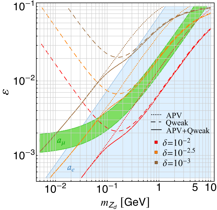
Figure 2: Limits at 90% CL in the plane of $m_{Z_{d}}$ and $\varepsilon$, for both ${\rm Q_{weak}}$ (dashed line) and APV (dotted line) experiments, and also their combination (solid line), for different values of $\delta$ as depicted in the label. The green band and the light blue area are the favored regions at 90% CL needed to explain the anomalous magnetic moment of the muon and of the electron, respectively.

We note that the ability to exclude the $a_{\mu}$ and $a_{e}$ interpretations under the $Z_{d}$ model depends strongly on the value of $\delta$ chosen. Namely, for $\delta>10^{-2}$ the entire $\Delta a_{\mu}$ discrepancy is completely ruled out, not only by the combined result but also by the APV only limit. Other experiments that are also sensitive to $Z_{d}$ bosons are those able to measure rare flavor-changing weak neutral-current decays of $K$ and $B$ mesons, like $K^{\pm}\to\pi^{\pm}Z_{d}$, induced by quark transition amplitudes such as $s\to dZ_{d}$ and $b\to sZ_{d}$ Davoudiasl et al. (2014); Essig et al. (2013); Izaguirre et al. (2013); Pospelov et al. (2008). Similarly, Higgs boson decays to $ZZ_{d}$ bosons Davoudiasl et al. (2012a, 2015), induced by $Z-Z_{d}$ mass mixing, are also sensitive to it. In both cases, the constraints obtained depend on the assumed branching fraction (BF) of the $Z_{d}$ boson decay and on its mass. Indeed, if only SM particles are lighter than the $Z_{d}$ boson, the latter could decay into pairs of charged leptons or hadrons, leaving a visible signature in detectors, or into a pair of neutrinos, resulting in missing energy. Instead, if it exists at least one dark-matter particle whose mass is such that $2m_{\chi}<m_{Z_{d}}$, the $Z_{d}$ boson decays preferentially into dark-matter, depending on the assumed coupling $\alpha_{D}$. In the mass range $30\lesssim m_{Z_{d}}\lesssim 300$ MeV the dominant constraints arise from rare kaon decays. Indeed, the BNL E949 experiment combined with the E787 results put severe constraints on $K^{+}\to\pi^{+}+$invisible Artamonov et al. (2009), that however can be significantly relaxed in case of $\delta\neq 0$ thanks to a cancellation that may occur between kinetic and $Z-Z_{d}$ mass mixing Davoudiasl et al. (2014). It is worth to mention that the two favored regions determined for the magnetic moments in Fig. 2 do not depend significantly on the value of $\delta$, at least for the small values tested in this work, since the dominant contribution is the one induced by the term related to the kinetic mixing parameter $\varepsilon$ in Eq. (8).

In Fig. 2 it is possible to see that, for given values of $\delta$, $m_{Z_{d}}$ and $\varepsilon$, there is an overlap between all the different experimental constraints. To better highlight it, we performed a combined fit by summing all the four $\chi^{2}$’s in Eq. (27). In order to remove the ambiguity on $\delta$, we marginalized the result over this parameter. In Fig. 3 we show the $1\sigma$, $2\sigma$, and $3\sigma$ CL contours in the plane of $m_{Z_{d}}$ and $\varepsilon$, as well as the best fit result corresponding to a minimum $\chi_{\mathrm{min}}^{2}=0.007$.

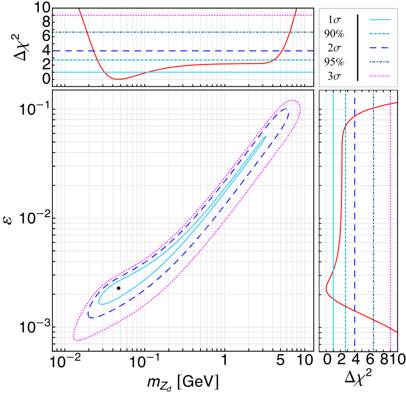
Figure 3: Contours at different CL of the allowed regions in the plane of $m_{Z_{d}}$ and $\varepsilon$, together with their marginalizations, obtained from the combined fit of the ${\rm Q_{weak}}$, APV, $a_{\mu}$ and $a_{e}$ experimental results. The best fit result is indicated by the black dot.

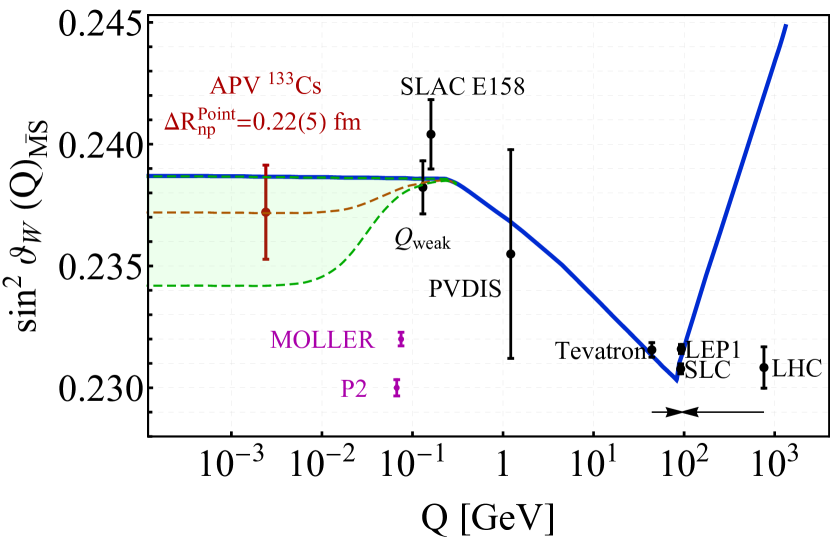
Figure 4: Variation of $\sin^{2}\vartheta_{\text{W}}$ with energy scale $Q$. The SM prediction is shown as the solid blue curve, together with experimental determinations in black Tanabashi et al. (2018); Wood et al. (1997); Dzuba et al. (2012); Anthony et al. (2005, 2005); Wang et al. (2014); Zeller et al. (2002); Androic et al. (2018) and future projections in violet Becker et al. (2018); Benesch et al. (2014) with a central value shown at an arbitrary position. The result derived in this paper for APV on cesium is shown in red. With the dashed red and green lines we indicate the best fit result and the $\pm 1\sigma$ variations, respectively, for the running of $\sin^{2}\vartheta_{\text{W}}$ in the presence of a $Z_{d}$ boson as described in the paper.

For completeness, when marginalizing in turn over the other two parameters, we get the following results for $m_{Z_{d}}$, $\varepsilon$ and $\delta$ at $1\sigma$ CL

$$m_{Z_{d}} =47{}^{+61}_{-16}\,\mathrm{MeV},$$ (28)

$$\varepsilon =2.3{}^{+1.1}_{-0.4}\times 10^{-3},$$ (29)

$$\delta <2\times 10^{-3}.$$ (30)

Using these best fit values and their $1\sigma$ ranges, in Fig. 4 we show how the running of $\sin^{2}\vartheta_{\text{W}}$ changes at low energies due to the contribution of a $Z_{d}$ boson. Clearly, further measurements of $\sin^{2}\vartheta_{\text{W}}$ in the low energy sector, as those coming from the P2 Becker et al. (2018); Dev et al. (2021) and MOLLER Benesch et al. (2014) experiments, from the near DUNE detector de Gouvea et al. (2020), the exploitation of coherent elastic neutrino scattering in atoms Cadeddu et al. (2019) and nuclei Cadeddu et al. (2020a); Fernandez-Moroni et al. (2021); Cañas et al. (2018) and finally from future atomic parity violation with francium, radium and rubidium Safronova et al. (2018); Roberts et al. (2015) would be really powerful for further constraining such a model.

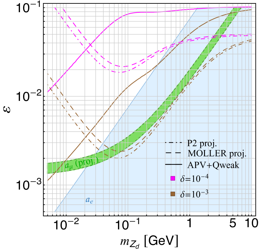
Figure 5: Limits at 90% CL in the plane of $m_{Z_{d}}$ and $\varepsilon$, for the combination of the current ${\rm Q_{weak}}$ and APV experiments (solid), the projected MOLLER (dashed) and P2 (dot-dashed) proposed experiments, for different values of $\delta$ as depicted in the label. The green band and the light blue area are the favored regions at 90% CL needed to explain the projected and current anomalous magnetic moment of the muon and of the electron, respectively.

To highlight the near future prospects that can be achieved thanks to upcoming results from MOLLER and P2, considering the SM value for the central value, as well as an improved measurement of $a_{\mu}$ with half of the uncertainty in Eq. (1), we show in Fig. 5 the limits at 90% CL in the plane of $m_{Z_{d}}$ and $\varepsilon$ for different values of $\delta$. As clearly visible, P2 and MOLLER will allow to exclude a large portion of the $a_{\mu}$ band already for values of $\delta$ as small as $10^{-3}$. See Ref. ref (2021) for additional information.

In summary, in this paper we studied a possible $U(1)_{d}$ extension of the SM that implies the presence of a sub-GeV-scale vector $Z_{d}$ mediator. The existence of this additional force would modify the experimental values of the muon and electron anomalous magnetic moments as well as the measurements of the proton and cesium weak charge, performed so far at low-energy transfer. Motivated by the recent determination of the muon anomalous magnetic moment performed at Fermilab, we derived the constraints on such a model obtained from the aforementioned experimental measurements and by their combination. Before to do so, we revisited the determination of the cesium $Q_{W}$ from the atomic parity violation experiment, which depends critically on the value of the average neutron rms radius of ${}^{133}\text{Cs}$, by determining the latter from a practically model-independent extrapolation from the recent average neutron rms radius of ${}^{208}\text{Pb}$ performed by the PREX-2 Collaboration. From a combined $\chi^{2}$ fit we obtain rather precise limits on the mass and the kinetic mixing parameter of the $Z_{d}$ boson, namely $m_{Z_{d}}=47{}^{+61}_{-16}\,\mathrm{MeV}$ and $\varepsilon=2.3{}^{+1.1}_{-0.4}\times 10^{-3}$, when marginalizing over the $Z-Z_{d}$ mass mixing parameter $\delta$.

References

- Bennett et al. (2006) G. W. Bennett, B. Bousquet, H. N. Brown, G. Bunce, R. M. Carey, P. Cushman, G. T. Danby, P. T. Debevec, M. Deile, H. Deng, and et al., Physical Review D 73 (2006), 10.1103/physrevd.73.072003.
- Abi et al. (2021) B. Abi et al. (Muon Collaboration), Phys. Rev. Lett. 126, 141801 (2021).
- Aoyama et al. (2020) T. Aoyama et al., Phys. Rept. 887, 1 (2020), arXiv:2006.04822 [hep-ph] .
- Aoyama et al. (2012) T. Aoyama, M. Hayakawa, T. Kinoshita, and M. Nio, Phys. Rev. Lett. 109, 111808 (2012), arXiv:1205.5370 [hep-ph] .
- Aoyama et al. (2019) T. Aoyama, T. Kinoshita, and M. Nio, Atoms 7, 28 (2019).
- Czarnecki et al. (2003) A. Czarnecki, W. J. Marciano, and A. Vainshtein, Phys. Rev. D67, 073006 (2003), [Erratum: Phys. Rev. D73, 119901 (2006)], arXiv:hep-ph/0212229 [hep-ph] .
- Gnendiger et al. (2013) C. Gnendiger, D. Stöckinger, and H. Stöckinger-Kim, Phys. Rev. D88, 053005 (2013), arXiv:1306.5546 [hep-ph] .
- Davier et al. (2017) M. Davier, A. Hoecker, B. Malaescu, and Z. Zhang, Eur. Phys. J. C77, 827 (2017), arXiv:1706.09436 [hep-ph] .
- Keshavarzi et al. (2018) A. Keshavarzi, D. Nomura, and T. Teubner, Phys. Rev. D97, 114025 (2018), arXiv:1802.02995 [hep-ph] .
- Colangelo et al. (2019) G. Colangelo, M. Hoferichter, and P. Stoffer, JHEP 02, 006 (2019), arXiv:1810.00007 [hep-ph] .
- Hoferichter et al. (2019) M. Hoferichter, B.-L. Hoid, and B. Kubis, JHEP 08, 137 (2019), arXiv:1907.01556 [hep-ph] .
- Davier et al. (2020) M. Davier, A. Hoecker, B. Malaescu, and Z. Zhang, Eur. Phys. J. C80, 241 (2020), [Erratum: Eur. Phys. J. C80, 410 (2020)], arXiv:1908.00921 [hep-ph] .
- Keshavarzi et al. (2020) A. Keshavarzi, D. Nomura, and T. Teubner, Phys. Rev. D101, 014029 (2020), arXiv:1911.00367 [hep-ph] .
- Melnikov and Vainshtein (2004) K. Melnikov and A. Vainshtein, Phys. Rev. D70, 113006 (2004), arXiv:hep-ph/0312226 [hep-ph] .
- Masjuan and Sánchez-Puertas (2017) P. Masjuan and P. Sánchez-Puertas, Phys. Rev. D95, 054026 (2017), arXiv:1701.05829 [hep-ph] .
- Colangelo et al. (2017) G. Colangelo, M. Hoferichter, M. Procura, and P. Stoffer, JHEP 04, 161 (2017), arXiv:1702.07347 [hep-ph] .
- Hoferichter et al. (2018) M. Hoferichter, B.-L. Hoid, B. Kubis, S. Leupold, and S. P. Schneider, JHEP 10, 141 (2018), arXiv:1808.04823 [hep-ph] .
- Gérardin et al. (2019) A. Gérardin, H. B. Meyer, and A. Nyffeler, Phys. Rev. D100, 034520 (2019), arXiv:1903.09471 [hep-lat] .
- Bijnens et al. (2019) J. Bijnens, N. Hermansson-Truedsson, and A. Rodríguez-Sánchez, Phys. Lett. B798, 134994 (2019), arXiv:1908.03331 [hep-ph] .
- Colangelo et al. (2020) G. Colangelo, F. Hagelstein, M. Hoferichter, L. Laub, and P. Stoffer, JHEP 03, 101 (2020), arXiv:1910.13432 [hep-ph] .
- Pauk and Vanderhaeghen (2014) V. Pauk and M. Vanderhaeghen, Eur. Phys. J. C74, 3008 (2014), arXiv:1401.0832 [hep-ph] .
- Danilkin and Vanderhaeghen (2017) I. Danilkin and M. Vanderhaeghen, Phys. Rev. D95, 014019 (2017), arXiv:1611.04646 [hep-ph] .
- Jegerlehner (2017) F. Jegerlehner, Springer Tracts Mod. Phys. 274, 1 (2017).
- Knecht et al. (2018) M. Knecht, S. Narison, A. Rabemananjara, and D. Rabetiarivony, Phys. Lett. B787, 111 (2018), arXiv:1808.03848 [hep-ph] .
- Eichmann et al. (2020) G. Eichmann, C. S. Fischer, and R. Williams, Phys. Rev. D101, 054015 (2020), arXiv:1910.06795 [hep-ph] .
- Roig and Sánchez-Puertas (2020) P. Roig and P. Sánchez-Puertas, Phys. Rev. D101, 074019 (2020), arXiv:1910.02881 [hep-ph] .
- Blum et al. (2020) T. Blum, N. Christ, M. Hayakawa, T. Izubuchi, L. Jin, C. Jung, and C. Lehner, Phys. Rev. Lett. 124, 132002 (2020), arXiv:1911.08123 [hep-lat] .
- Colangelo et al. (2014) G. Colangelo, M. Hoferichter, A. Nyffeler, M. Passera, and P. Stoffer, Phys. Lett. B735, 90 (2014), arXiv:1403.7512 [hep-ph] .
- Aaij et al. (2021) R. Aaij et al. (LHCb), “Test of lepton universality in beauty-quark decays,” (2021), arXiv:2103.11769 [hep-ex] .
- Hanneke et al. (2008) D. Hanneke, S. Fogwell, and G. Gabrielse, Physical Review Letters 100 (2008), 10.1103/physrevlett.100.120801.
- Hanneke et al. (2011) D. Hanneke, S. Fogwell Hoogerheide, and G. Gabrielse, Physical Review A 83 (2011), 10.1103/physreva.83.052122.
- Parker et al. (2018) R. H. Parker, C. Yu, W. Zhong, B. Estey, and H. Müller, Science 360, 191–195 (2018).
- Morel et al. (2020) L. Morel, Z. Yao, P. Cladé, and S. Guellati-Khélifa, Nature 588, 61 (2020).
- Fayet (2007) P. Fayet, Physical Review D 75 (2007), 10.1103/physrevd.75.115017.
- Davoudiasl and Marciano (2018) H. Davoudiasl and W. J. Marciano, Physical Review D 98 (2018), 10.1103/physrevd.98.075011.
- Cadeddu et al. (2021a) M. Cadeddu, N. Cargioli, F. Dordei, C. Giunti, Y. F. Li, E. Picciau, and Y. Y. Zhang, JHEP 01, 116 (2021a), arXiv:2008.05022 [hep-ph] .
- Bœhm and Fayet (2004) C. Bœhm and P. Fayet, Nuclear Physics B 683, 219–263 (2004).
- Giudice et al. (2012) G. F. Giudice, P. Paradisi, and M. Passera, Journal of High Energy Physics 2012 (2012), 10.1007/jhep11(2012)113.
- Bodas et al. (2021) A. Bodas, R. Coy, and S. J. D. King, “Solving the electron and muon anomalies in models,” (2021), arXiv:2102.07781 [hep-ph] .
- Davoudiasl et al. (2012a) H. Davoudiasl, H.-S. Lee, and W. J. Marciano, Physical Review D 85 (2012a), 10.1103/physrevd.85.115019.
- Davoudiasl et al. (2012b) H. Davoudiasl, H.-S. Lee, and W. J. Marciano, Physical Review D 86 (2012b), 10.1103/physrevd.86.095009.
- Davoudiasl et al. (2013) H. Davoudiasl, H.-S. Lee, I. Lewis, and W. J. Marciano, Physical Review D 88 (2013), 10.1103/physrevd.88.015022.
- Arcadi et al. (2019) G. Arcadi, M. Lindner, J. Martins, and F. S. Queiroz, “New physics probes: Atomic parity violation, polarized electron scattering and neutrino-nucleus coherent scattering,” (2019), arXiv:1906.04755 [hep-ph] .
- Davoudiasl et al. (2015) H. Davoudiasl, H.-S. Lee, and W. J. Marciano, Physical Review D 92 (2015), 10.1103/physrevd.92.055005.
- Zyla et al. (2020) P. Zyla et al. (Particle Data Group), PTEP 2020, 083C01 (2020).
- Erler and Ramsey-Musolf (2005) J. Erler and M. J. Ramsey-Musolf, Phys. Rev. D72, 073003 (2005), arXiv:hep-ph/0409169 [hep-ph] .
- Erler and Ferro-Hernández (2018) J. Erler and R. Ferro-Hernández, JHEP 03, 196 (2018), arXiv:1712.09146 [hep-ph] .
- Davoudiasl et al. (2012c) H. Davoudiasl, H.-S. Lee, and W. J. Marciano, Physical Review Letters 109 (2012c), 10.1103/physrevlett.109.031802.
- Davoudiasl et al. (2014) H. Davoudiasl, H.-S. Lee, and W. J. Marciano, Phys. Rev. D 89, 095006 (2014), arXiv:1402.3620 [hep-ph] .
- Bouchiat and Piketty (1983) C. Bouchiat and C. Piketty, Physics Letters B 128, 73 (1983).
- Bouchiat and Fayet (2005) C. Bouchiat and P. Fayet, Physics Letters B 608, 87–94 (2005).
- Davoudiasl et al. (2012d) H. Davoudiasl, H.-S. Lee, and W. J. Marciano, Phys. Rev. Lett. 109, 031802 (2012d).
- Androic et al. (2018) D. Androic et al. (Qweak), Nature 557, 207 (2018).
- Erler and Su (2013) J. Erler and S. Su, Prog. Part. Nucl. Phys. 71, 119 (2013), arXiv:1303.5522 [hep-ph] .
- Wood et al. (1997) C. S. Wood, S. C. Bennett, D. Cho, B. P. Masterson, J. L. Roberts, C. E. Tanner, and C. E. Wieman, Science 275, 1759 (1997).
- Guena et al. (2005) J. Guena, M. Lintz, and M. A. Bouchiat, Phys. Rev. A 71, 042108 (2005), arXiv:physics/0412017 .
- Pollock and Welliver (1999) S. Pollock and M. Welliver, Physics Letters B 464, 177–182 (1999).
- Pollock et al. (1992) S. J. Pollock, E. N. Fortson, and L. Wilets, Phys. Rev. C 46, 2587 (1992).
- Horowitz et al. (2001) C. J. Horowitz, S. J. Pollock, P. A. Souder, and R. Michaels, Physical Review C 63 (2001), 10.1103/physrevc.63.025501.
- Dzuba et al. (2012) V. A. Dzuba, J. C. Berengut, V. V. Flambaum, and B. Roberts, Phys. Rev. Lett. 109, 203003 (2012), arXiv:1207.5864 [hep-ph] .
- Derevianko (2001) A. Derevianko, Phys. Rev. A 65, 012106 (2001).
- Trzcińska et al. (2001) A. Trzcińska, J. Jastrzȩbski, P. Lubiński, F. J. Hartmann, R. Schmidt, T. von Egidy, and B. Kłos, Phys. Rev. Lett. 87, 082501 (2001).
- Johnson and Soff (1985) W. Johnson and G. Soff, Atomic Data and Nuclear Data Tables 33, 405 (1985).
- Thiel et al. (2019) M. Thiel, C. Sfienti, J. Piekarewicz, C. J. Horowitz, and M. Vanderhaeghen, J. Phys. G 46, 093003 (2019), arXiv:1904.12269 [nucl-ex] .
- Horowitz et al. (2012) C. J. Horowitz et al., Phys. Rev. C 85, 032501 (2012), arXiv:1202.1468 [nucl-ex] .
- Adhikari et al. (2021) D. Adhikari et al. (PREX), Phys. Rev. Lett. 126, 172502 (2021), arXiv:2102.10767 [nucl-ex] .
- Abrahamyan et al. (2012) S. Abrahamyan, Z. Ahmed, H. Albataineh, K. Aniol, D. S. Armstrong, W. Armstrong, T. Averett, B. Babineau, A. Barbieri, V. Bellini, and et al., Physical Review Letters 108 (2012), 10.1103/physrevlett.108.112502.
- Reed (2020) B. Reed, Presentation on behalf of the PREX-II Collaboration at the Magnificent CEvNS 2020 workshop (2020).
- Dobaczewski et al. (1984) J. Dobaczewski, H. Flocard, and J. Treiner, Nucl. Phys. A422, 103 (1984).
- Bartel et al. (1982) J. Bartel, P. Quentin, M. Brack, C. Guet, and H. B. Hakansson, Nucl. Phys. A386, 79 (1982).
- Kortelainen et al. (2012) M. Kortelainen, J. McDonnell, W. Nazarewicz, P. G. Reinhard, J. Sarich, N. Schunck, M. V. Stoitsov, and S. M. Wild, Phys. Rev. C85, 024304 (2012), arXiv:1111.4344 [nucl-th] .
- Kortelainen et al. (2010) M. Kortelainen, T. Lesinski, J. More, W. Nazarewicz, J. Sarich, N. Schunck, M. V. Stoitsov, and S. Wild, Phys. Rev. C82, 024313 (2010), arXiv:1005.5145 [nucl-th] .
- Chabanat et al. (1998) E. Chabanat, P. Bonche, P. Haensel, J. Meyer, and R. Schaeffer, Nucl. Phys. A635, 231 (1998).
- Reinhard and Flocard (1995) P. G. Reinhard and H. Flocard, Nucl. Phys. A584, 467 (1995).
- Hernandez (2019) J. A. Hernandez, Weak Nuclear Form Factor: Nuclear Structure Coherent Elastic Neutrino-Nucleus Scattering, Master’s thesis, Florida State U., Tallahassee (main) (2019).
- Yang et al. (2019) J. Yang, J. A. Hernandez, and J. Piekarewicz, Phys. Rev. C 100, 054301 (2019), arXiv:1908.10939 [nucl-th] .
- Chen and Piekarewicz (2014) W.-C. Chen and J. Piekarewicz, Phys. Rev. C 90, 044305 (2014), arXiv:1408.4159 [nucl-th] .
- Chen and Piekarewicz (2015) W.-C. Chen and J. Piekarewicz, Phys. Lett. B 748, 284 (2015), arXiv:1412.7870 [nucl-th] .
- Sharma et al. (1993) M. M. Sharma, M. A. Nagarajan, and P. Ring, Phys. Lett. B312, 377 (1993).
- Bender et al. (1999) M. Bender, K. Rutz, P. G. Reinhard, J. A. Maruhn, and W. Greiner, Phys. Rev. C60, 034304 (1999), nucl-th/9906030 [nucl-th] .
- Lalazissis et al. (1997) G. A. Lalazissis, J. Konig, and P. Ring, Phys. Rev. C55, 540 (1997), nucl-th/9607039 [nucl-th] .
- Reinhard et al. (1986) P. G. Reinhard, M. Rufa, J. Maruhn, W. Greiner, and J. Friedrich, Z. Phys. A 323, 13 (1986).
- Niksic et al. (2008) T. Niksic, D. Vretenar, and P. Ring, Phys. Rev. C78, 034318 (2008), arXiv:0809.1375 [nucl-th] .
- Niksic et al. (2002) T. Niksic, D. Vretenar, P. Finelli, and P. Ring, Phys. Rev. C66, 024306 (2002), nucl-th/0205009 [nucl-th] .
- Zheng et al. (2014) H. Zheng, Z. Zhang, and L.-W. Chen, JCAP 08, 011 (2014), arXiv:1403.5134 [nucl-th] .
- Sil et al. (2005) T. Sil, M. Centelles, X. Vinas, and J. Piekarewicz, Phys. Rev. C 71, 045502 (2005), arXiv:nucl-th/0501014 .
- Piekarewicz et al. (2012) J. Piekarewicz, B. K. Agrawal, G. Colò, W. Nazarewicz, N. Paar, P.-G. Reinhard, X. Roca-Maza, and D. Vretenar, Phys. Rev. C 85, 041302 (2012).
- Yue et al. (2021) T.-G. Yue, L.-W. Chen, Z. Zhang, and Y. Zhou, “Constraints on the Symmetry Energy from PREX-II in the Multimessenger Era,” (2021), arXiv:2102.05267 [nucl-th] .
- Cadeddu et al. (2021b) M. Cadeddu, N. Cargioli, F. Dordei, C. Giunti, Y. F. Li, E. Picciau, C. A. Ternes, and Y. Y. Zhang, “New insights into nuclear physics and weak mixing angle using electroweak probes,” (2021b), arXiv:2102.06153 [hep-ph] .
- Fricke et al. (1995) G. Fricke, C. Bernhardt, K. Heilig, L. A. Schaller, L. Schellenberg, E. B. Shera, and C. W. de Jager, Atom. Data Nucl. Data Tabl. 60, 177 (1995).
- Angeli and Marinova (2013) I. Angeli and K. P. Marinova, Atom. Data Nucl. Data Tabl. 99, 69 (2013).
- Cadeddu and Dordei (2019) M. Cadeddu and F. Dordei, Phys. Rev. D 99, 033010 (2019), arXiv:1808.10202 [hep-ph] .
- Cadeddu et al. (2020a) M. Cadeddu, F. Dordei, C. Giunti, Y. Li, E. Picciau, and Y. Zhang, Phys. Rev. D 102, 015030 (2020a), arXiv:2005.01645 [hep-ph] .
- Hoferichter et al. (2020) M. Hoferichter, J. Menéndez, and A. Schwenk, Physical Review D 102 (2020), 10.1103/physrevd.102.074018.
- Viatkina et al. (2019) A. V. Viatkina, D. Antypas, M. G. Kozlov, D. Budker, and V. V. Flambaum, Phys. Rev. C 100, 034318 (2019).
- Cadeddu et al. (2020b) M. Cadeddu, F. Dordei, C. Giunti, Y. F. Li, and Y. Y. Zhang, Phys. Rev. D101, 033004 (2020b), arXiv:1908.06045 [hep-ph] .
- Essig et al. (2013) R. Essig, J. Mardon, M. Papucci, T. Volansky, and Y.-M. Zhong, JHEP 11, 167 (2013), arXiv:1309.5084 [hep-ph] .
- Izaguirre et al. (2013) E. Izaguirre, G. Krnjaic, P. Schuster, and N. Toro, Phys. Rev. D 88, 114015 (2013), arXiv:1307.6554 [hep-ph] .
- Pospelov et al. (2008) M. Pospelov, A. Ritz, and M. B. Voloshin, Phys. Lett. B 662, 53 (2008), arXiv:0711.4866 [hep-ph] .
- Artamonov et al. (2009) A. V. Artamonov et al. (BNL-E949), Phys. Rev. D 79, 092004 (2009), arXiv:0903.0030 [hep-ex] .
- Tanabashi et al. (2018) M. Tanabashi et al. (Particle Data Group), Phys. Rev. D98, 030001 (2018).
- Anthony et al. (2005) P. L. Anthony et al. (SLAC E158), Phys. Rev. Lett. 95, 081601 (2005), hep-ex/0504049 [hep-ex] .
- Wang et al. (2014) D. Wang et al. (PVDIS), Nature 506, 67 (2014).
- Zeller et al. (2002) G. P. Zeller et al. (NuTeV), Phys. Rev. Lett. 88, 091802 (2002), hep-ex/0110059 .
- Becker et al. (2018) D. Becker et al., Eur. Phys. J. A 54, 208 (2018), arXiv:1802.04759 [nucl-ex] .
- Benesch et al. (2014) J. Benesch et al. (MOLLER), “The MOLLER Experiment: An Ultra-Precise Measurement of the Weak Mixing Angle Using Moller Scattering,” (2014), arXiv:1411.4088 [nucl-ex] .
- ref (2021) “See Supplemental Material at http://link.aps.org/supplemental/10.1103/PhysRevD.104.L011701 for more information,” (2021).
- Dev et al. (2021) P. S. B. Dev, W. Rodejohann, X.-J. Xu, and Y. Zhang, “Searching for bosons at the P2 experiment,” (2021), arXiv:2103.09067 [hep-ph] .
- de Gouvea et al. (2020) A. de Gouvea, P. A. N. Machado, Y. F. Perez-Gonzalez, and Z. Tabrizi, Phys. Rev. Lett. 125, 051803 (2020), arXiv:1912.06658 [hep-ph] .
- Cadeddu et al. (2019) M. Cadeddu, F. Dordei, C. Giunti, K. Kouzakov, E. Picciau, and A. Studenikin, Physical Review D 100 (2019), 10.1103/physrevd.100.073014.
- Fernandez-Moroni et al. (2021) G. Fernandez-Moroni, P. A. N. Machado, I. Martinez-Soler, Y. F. Perez-Gonzalez, D. Rodrigues, and S. Rosauro-Alcaraz, Journal of High Energy Physics 2021 (2021), 10.1007/jhep03(2021)186.
- Cañas et al. (2018) B. Cañas, E. Garcés, O. Miranda, and A. Parada, Physics Letters B 784, 159–162 (2018).
- Safronova et al. (2018) M. S. Safronova, D. Budker, D. DeMille, D. F. J. Kimball, A. Derevianko, and C. W. Clark, Rev. Mod. Phys. 90, 025008 (2018).
- Roberts et al. (2015) B. Roberts, V. Dzuba, and V. Flambaum, Annual Review of Nuclear and Particle Science 65, 63–86 (2015).