Analytical results for the low-temperature Drude weight of the XXZ spin chain

Abstract

The spin-$1/2$ XXZ chain is an integrable lattice model and parts of its spin current can be protected by local conservation laws for anisotropies $-1<\Delta<1$. In this case, the Drude weight $D(T)$ is non-zero at finite temperatures $T$. Here we obtain analytical results for $D(T)$ at low temperatures for zero external magnetic field and anisotropies $\Delta=\cos(n\pi/m)$ with $n,m$ coprime integers, using the thermodynamic Bethe ansatz. We show that to leading orders $D(T)=D(0)-a(\Delta)T^{2K-2}-b_{1}(\Delta)T^{2}$ where $K$ is the Luttinger parameter and the prefactor $a(\Delta)$, obtained in closed form, has a fractal structure as function of anisotropy $\Delta$. The prefactor $b_{1}(\Delta)$, on the other hand, does not have a fractal structure and can be obtained in a standard field-theoretical approach. Including both temperature corrections, we obtain an analytic result for the low-temperature asymptotics of the Drude weight in the entire regime $-1<\Delta=\cos(n\pi/m)<1$.

I Introduction

One-dimensional integrable quantum systems can exhibit unusual transport properties [1, 2, 3, 4, 5, 6, 7, 8, 9, 10], which are, in principle, exactly computable by the Bethe ansatz. Bethe ansatz and related techniques have been used to successfully investigate many different aspects of these models [11, 4, 5, 6, 12, 13, 14, 9, 15, 16, 17]. More recently, the advent of generalized hydrodynamics (GHD) [18, 19, 20, 21] has provided a new avenue to explore their transport properties. GHD combines the thermodynamic Bethe ansatz (TBA) [22] with a continuity equation and an assumed form for the current operator, which has been demonstrated to be exact in Refs. [23, 24, 25] on the level of form factors. By use of a projective formalism [26], formulas for the Drude weight [20, 27] and diffusion coefficients [28, 29, 30] have been determined from GHD. For the XXZ spin chain, these formulas for the Drude weight do agree with the result derived 20 years earlier by Zotos [4] which relies only on the TBA. So far, however, analytical results for the Drude weight are only available at zero temperature [1] and at infinite temperature [9, 31, 32]. For finite temperatures, on the other hand, these approaches lead to a set of equations that have only been solved numerically up to now. The objective of this paper is to obtain closed-form expressions for the Drude weight of the XXZ chain at low temperatures and zero magnetic field.

The Hamiltonian of the XXZ spin chain is given by

$$H=\sum_{l=1}^{M}\left\{\frac{J}{4}\left(\sigma^{x}_{l}\sigma^{x}_{l+1}+\sigma^{y}_{l}\sigma^{y}_{l+1}+\Delta\sigma^{z}_{l}\sigma^{z}_{l+1}\right)-\frac{h}{2}\sigma^{z}_{l}\right\}\,,$$ (1)

where $J$ is the exchange constant, $M$ the number of lattice sites, $\sigma^{x,y,z}$ are Pauli matrices, and $\Delta=\cos(\gamma)$ the anisotropy parametrized by $\gamma$. The magnetic field is denoted by $h$ and we use periodic boundary conditions. The XXZ chain is a quantum integrable model which has a family of commuting transfer matrices, $[T(\theta),T(\theta^{\prime})]=0$ with $\theta$, $\theta^{\prime}$ being spectral parameters. These transfer matrices generate an infinite set of local conserved charges $Q_{n}$, which are obtained by

$$Q_{n}=\frac{d^{n}}{d\theta^{n}}\ln T(\theta)\bigg{|}_{\theta=0}.$$ (2)

In particular, $Q_{1}\propto H$ and $Q_{2}\propto J_{E}$ where $J_{E}$ is the energy current operator. Because $J_{E}$ itself is conserved, the thermal conductivity in linear response can be calculated straightforwardly from a generalized Gibbs ensemble (GGE), which includes the higher conserved charges [5, 33]. Spin transport in the XXZ chain, on the other hand, is much more complicated to investigate because the spin current operator $J_{0}$ is not conserved [2].

Our paper is organized as follows: in Sec. II we present different approaches to calculate spin transport in linear response. In Sec. III we review the asymptotic analysis of a system of non-linear integral equations for the free energy of the XXZ chain. We then show in Sec. IV that a similar asymptotic analysis can also be performed for the Fermi weight. Using the derived asymptotic formulas for the Fermi weight, we then obtain in Sec. V an analytic low-temperature expansion of $D(T)$ at the simple roots of unity, i.e., anisotropies $\gamma=\pi/m$. The generalization to anisotropies $\gamma=n\pi/m$ is discussed in Sec. VI. By including the leading temperature correction with integer scaling dimension known from field theory and comparing to a numerical solution of the TBA equations, we show in Sec. VII that the obtained analytical asymptotics describes the Drude weight correctly at low temperatures in the entire regime $-1<\Delta=\cos(n\pi/m)<1$. The final section is devoted to a short summary and some conclusions.

II Drude weight

The spin Drude weight can be defined in the following two equivalent ways. Firstly, using the Kubo formalism the spin conductivity $\sigma(\omega)$ as a function of frequency $\omega$ can be expressed in linear response as

$$\sigma(\omega)=\frac{\mathrm{i}}{\omega}\left[\frac{\langle E_{\text{kin}}\rangle}{N}+\langle J_{0},J_{0}\rangle_{\text{ret}}(\omega)\right].$$ (3)

Here $\langle E_{\text{kin}}\rangle$ is the expectation value of the kinetic energy of the Hamiltonian and $\langle J_{0},J_{0}\rangle_{\text{ret}}(\omega)$ denotes the retarded current-current correlation function. The current operator is given by $J_{0}=\sum_{l}j_{l}$ with

$$j_{l}=\mathrm{i}J\left(\sigma^{+}_{l}\sigma^{-}_{l+1}-h.c.\right)$$ (4)

and $\sigma^{\pm}=(\sigma^{x}\pm\mathrm{i}\sigma^{y})/2$. The real part of the conductivity can then be written as

$$\sigma^{\prime}(\omega)=2\pi D(T)\delta(\omega)+\sigma_{\text{reg}}(T,\omega),$$ (5)

where a non-zero Drude weight $D(T)$ implies an infinite dc conductivity at a given temperature $T$ and $\sigma_{\text{reg}}(T,\omega)$ is the regular part of the conductivity.

A second expression relates the Drude weight directly to the real-time current-current correlator and the conserved charges $Q_{k}$ of the XXZ chain as

$$2TD=\lim_{t\to\infty}\lim_{N\to\infty}\frac{\langle J_{0}(0)J_{0}(t)\rangle}{N}\geq\lim_{N\to\infty}\sum_{k}\frac{|\langle J_{0}Q_{k}\rangle|^{2}}{N\langle Q^{\dagger}_{k}Q_{k}\rangle}.$$ (6)

The first equation gives a nice physical interpretation of the Drude weight. It shows that the Drude weight measures the part of the current with no decay in time. In the second inequality, a set of conserved charges $[H,Q_{k}]=0$ with $\langle Q_{k}Q_{l}\rangle=\delta_{kl}$ is inserted, making the projection onto the conserved part explicit. If only some of the conserved charges are taken into account then a lower bound, the so-called Mazur bound, is obtained [34]. The spin current (4) is odd under spin-flip symmetry $\sigma^{z}\to-\sigma^{z}$ while all the conserved charges obtained from Eq. (2) are even when $h=0$. These local charges therefore have no overlap with the current operator at zero magnetic field. In addition, there exist, however, also quasi-local charges for $\gamma=n\pi/m\in\mathbb{Q}$ with $n,m$ coprime obtained from transfer matrices when a general highest weight representation in auxiliary space is chosen instead of the standard spin-$1/2$ representation [9, 31, 32]. Completeness of the set of local and quasi-local conserved charges is believed to be a consequence of the underlying quantum group [35], and taking all the symmetries into account turns the Mazur bound in Eq. (6) into an equality [34].

For anisotropies $\gamma/\pi=n/m\in\mathbb{Q}$ with $n,m$ coprime the Drude weight can be computed by multiple methods. The first amounts to a generalization of the Kohn formula [36] to finite temperatures [3]. By threading a static magnetic flux $\Phi$ through an XXZ ring and relating the now shifted eigenenergies $\epsilon_{n}$ to the Kubo formula (3) one finds

$$D=\frac{1}{2NZ}\sum_{n}\text{e}^{-\epsilon_{n}/T}\frac{\partial^{2}\epsilon_{n}(\Phi)}{\partial\Phi^{2}}\Big{\rvert}_{\Phi=0},$$ (7)

with $Z$ being the partition function. Using the TBA formalism [22], this method has been used in Ref. [4] to obtain the explicit formula (8) below, which we will call Zotos’ formula from here on. The second method is based on GHD and the Mazur bound. Assuming that the set of charges is complete, Zotos’ formula is reproduced. The third method is to explicitly construct the conserved charges. The difficulty then is to calculate overlaps of these charges with the current operator as well as the norm of these charges at finite temperatures. So far, this program has only been carried out explicitly at infinite temperatures [9, 31, 32].

The result of the first two methods is Zotos’ formula [4, 13] which can be expressed in terms of hole/particle ratios $\eta_{\ell}=\rho^{h}_{\ell}/\rho_{\ell}$ and factors $\sigma_{\ell}=\frac{\widetilde{\epsilon_{\ell}}}{|\widetilde{\epsilon_{\ell}}|}=\pm 1$, where $\widetilde{\epsilon_{\ell}}$ are the dressed quasi-particle energies. Zotos’ formula for the spin Drude weight can be written in terms of only the last two strings (particle and hole), which give identical contributions. For simplicity, we rewrite the Drude weight in terms of only the $L-1$ string, identified as the particle string, with $\eta=\eta_{L-1}$ and $\sigma=\sigma_{L-1}$ resulting in

$$D=-\frac{J\sin\gamma}{2\pi\gamma\beta}\sigma\int_{-\infty}^{\infty}d\theta\frac{\left(\partial_{\theta}\ln\eta\right)^{2}}{\partial_{\beta}\ln\eta}\frac{\eta\left(\partial_{\beta h}\ln\eta\right)^{2}}{(1+\eta)^{2}}.$$ (8)

In the infinite temperature limit, the above formula can be expanded to leading order in inverse temperature [13, 37]. The expansion is consistent with results obtained by an explicit construction of the conserved charges [31]

$$16TD(\infty)=\frac{J^{2}\sin^{2}\gamma}{\sin^{2}\left(\frac{\pi}{m}\right)}\left(1-\frac{m}{2\pi}\sin\left(\frac{2\pi}{m}\right)\right),$$ (9)

which, interestingly, is fractal in the anisotropy $\gamma=\frac{n\pi}{m}$. This is in contrast to the $T=0$ case, where the Drude weight can be obtained simply from the Kohn formula, Eq. (7), because only the curvature of the ground state energy level contributes. The continuous result is [1]

$$D(0)=\frac{v_{0}K}{4\pi},$$ (10)

where the Luttinger parameter $K=\frac{\pi}{\pi-\gamma}$ and spinon velocity $v_{0}=\frac{J\pi\sin\gamma}{2\gamma}$ are determined from the Bethe ansatz. We note that both the infinite temperature result (9) and the zero temperature result (10) are symmetric under $\gamma\to\pi-\gamma$ ($\Delta\to-\Delta$). This is, however, not true for finite temperatures and the regimes of positive and negative $\Delta$ both have to be analyzed.

A numerical evaluation of Zotos’ formula (8) suggests that for $T>0$ the zero field Drude weight is always fractal similar to the infinite temperature case and that the leading low-temperature correction for $0<\Delta<1$ scales as $T^{2K-2}$ [4], while the leading correction for $-1<\Delta\leq 0$ scales as $T^{2}$. The low-temperature behavior has also been investigated by a combined bosonization and memory matrix approach [8, 7, 38], which predicts that at finite temperatures a ballistic and a diffusive channel coexist. In this approach, Umklapp scattering is responsible for partially melting the Drude peak at finite temperatures with the difference going into the regular part of the conductance. However, the temperature dependence of the Drude weight cannot easily be obtained because it is related to the overlap of the current operator with the quasi-local charges. The representation of the latter in field theory is still an open issue.

Here, analytical results for the low-temperature Drude weight will be obtained directly from Zotos’ formula, supplemented by a field theory approach for the leading temperature correction with integer exponent. A combined auxiliary function [39] and TBA approach [22] will be taken. Our calculation makes use of the relationship between the $\eta$ functions and the quantum transfer matrix method in terms of the Y-system and T-systems defined in Ref. [40] via the fusion hierarchy, taking advantage of the simplest parts of both approaches.

Let us first rewrite Eq. (8) in a form which is more amenable to a low-temperature asymptotic analysis. In the following we set $J=1$. The integrand in Eq. (8) is simplified by noting that $\partial_{\beta h}\ln\eta=\frac{m}{2}$ and identifying an effective velocity

$$v=-\frac{\sin\gamma}{\beta\gamma}\frac{\partial_{\theta}\ln\eta}{\partial_{\beta}\ln\eta}$$ (11)

leading to

$$D=-\frac{m^{2}\sigma}{4\pi}\int_{0}^{\infty}d\theta\,v\,\partial_{\theta}\vartheta$$ (12)

with the Fermi weight $\vartheta(\theta)=(1+\eta(\theta))^{-1}$. An integration by parts yields

$$D=-\frac{m^{2}\sigma}{4\pi}\left(\vartheta(\infty)v_{0}-\int_{0}^{\infty}d\theta\,\vartheta\,\partial_{\theta}v\right),$$ (13)

with $v(\infty)=v_{0}$ and $v(0)=0$. The velocity changes rapidly around $\theta=0$, changing from the left to the right moving spinon velocity. This implies that the low-temperature Drude weight is dominated by the region $\theta\sim 0$. In the following, we are setting up the formalism to carry out an asymptotic analysis of this region.

III Non-linear Integral Equations

A particularly useful approach to determine the asymptotics of thermodynamic quantities is based on a set of non-linear integral equations (NLIE). For the XXZ chain, they were originally derived in Ref. [41] and again in Ref. [42]. All thermodynamic quantities can be expressed in terms of auxiliary functions $\mathfrak{a}$, $\bar{\mathfrak{a}}$, and associated functions $\ln A=\ln(1+\mathfrak{a})$, $\ln\bar{A}=\ln(1+\bar{\mathfrak{a}})$, which are related to each other by

$$\ln\mathfrak{a} =-e_{0}\beta+\kappa\star\ln A-\kappa^{2\mathrm{i}}\star\ln\bar{A},\,$$

$$\ln\bar{\mathfrak{a}} =-e_{0}\beta+\kappa\star\ln\bar{A}-\kappa^{-2\mathrm{i}}\star\ln A\,,$$ (14)

with $g^{\mathrm{i}c}=g(\theta+\mathrm{i}c)$. Here $(\kappa^{\mathrm{i}c}\star f)(\theta)=\int_{-\infty}^{\infty}d\mu\,\kappa(\theta-\mu+\mathrm{i}c)f(\mu)$ denotes a convolution with $c$ as a real number. The kernel is given by

$$\kappa(\theta)=\int\frac{dk}{2\pi}\frac{\sinh\left((p_{0}-2)k\right)e^{\mathrm{i}k\theta}}{2\cosh(k)\sinh\left((p_{0}-1)k\right)}$$ (15)

with $p_{0}=\frac{\pi}{\gamma}$, and $e_{0}=\frac{v_{0}}{\cosh\left(\frac{\pi}{2}\theta\right)}$. The main benefit of these NLIE is that the two auxiliary functions contain all the thermodynamic information of the model, which is in contrast with the large number of functions appearing in the usual TBA formalism.

At low-temperatures, the auxiliary functions rapidly change around $\theta\sim\mathcal{L}=\frac{2}{\pi}\ln(v_{0}\beta)$. By introducing the shift $\theta\to\theta+\mathcal{L}$ the temperature dependence will enter the rapidity directly [14]. After shifting the arguments in the NLIEs the contributions from the negative and positive parts of the real axis may be separately considered. For Eq. (III) we find, in particular,

$$\ln \mathfrak{a} =-e_{0}\beta+\int^{\infty}_{0}d\mu\left[\kappa(\theta-\mu)\ln A(\mu)-\kappa^{2\mathrm{i}}(\theta-\mu)\ln\bar{A}(\mu)+\kappa(\theta+\mu)\ln A(-\mu)-\kappa^{2\mathrm{i}}(\theta+\mu)\ln\bar{A}(-\mu)\right],$$

$$\ln \mathfrak{a}^{\mathcal{L}} \sim-2\text{e}^{-\theta\frac{\pi}{2}}+\int^{\infty}_{0}d\mu\left[\kappa^{\mathcal{L}}(\theta-\mu)\ln A(\mu)+\kappa^{\mathcal{L}}(\theta+\mu)\ln A(-\mu)-\kappa^{\mathcal{L}+2\mathrm{i}}(\theta-\mu)\ln\bar{A}(\mu)-\kappa^{\mathcal{L}+2\mathrm{i}}(\theta+\mu)\ln\bar{A}(-\mu)\right]$$ (16)

$$=-2\text{e}^{-\theta\frac{\pi}{2}}+\int^{\infty}_{-\mathcal{L}}d\mu\left[\kappa(\theta-\mu)\ln A_{+}(\mu)-\kappa^{2\mathrm{i}}(\theta-\mu)\ln\bar{A}_{+}(\mu)+\kappa^{2\mathcal{L}}(\theta+\mu)\ln A_{-}(\mu)-\kappa^{2\mathcal{L}+2\mathrm{i}}(\theta+\mu)\ln\bar{A}_{-}(\mu)\right]$$

$$=-2\text{e}^{-\theta\frac{\pi}{2}}+\int^{\infty}_{-\mathcal{L}}d\mu\left(\kappa(\theta-\mu)\ln A_{+}(\mu)-\kappa^{2\mathrm{i}}(\theta-\mu)\ln\bar{A}_{+}(\mu)\right)+\psi(\theta+2\mathcal{L}),$$

with $\ln A_{\pm}(\mu)=\ln A(\pm\mu\pm\mathcal{L})$. On the second line, we substituted $\theta\to\theta+\mathcal{L}$ resulting in $e_{0}=\frac{v_{0}}{\cosh\frac{\pi}{2}\theta}\to\frac{2}{\beta}\text{e}^{-\frac{\pi}{2}\theta}$, and on the third line $\mu\to\mu+\mathcal{L}$. We introduce the function $\psi(\theta+2\mathcal{L})$ on the fourth line, which contains sub-leading temperature contributions.

As a preparation for calculating the low-temperature Drude weight, we will first rederive the low-temperature asymptotics of the free energy $f(T)$. Our calculations for the Fermi weight $\vartheta(T)$ in Eq. (13) will proceed along similar lines. At low-temperatures, the auxiliary functions along the right/ left of the real axis are related to the free energy as [14]

$$f = e_{0}-\frac{T}{4}\int_{-\infty}^{\infty}d\theta\frac{\ln|A\bar{A}|}{\cosh\left(\frac{\pi}{2}\theta\right)}$$ (17)

$$= e_{0}-\frac{T^{2}}{2v_{0}}\int_{-\mathcal{L}}d\theta\frac{\ln|A_{+}A_{-}\bar{A}_{+}\bar{A}_{-}|}{\text{e}^{\pi\theta/2}}+O(T^{4})$$

$$\sim e_{0}-\frac{T^{2}}{v_{0}}\int_{-\mathcal{L}}d\theta\,\text{e}^{-\pi\theta/2}\ln|A_{+}\bar{A}_{+}|,$$

where $e_{0}$ is the ground state energy. The final line follows by identifying $\ln A_{\pm}=\ln\bar{A}_{\mp}$. This free energy relation can be used to construct a useful identity. First, we note that the asymptotic limits of the auxiliary functions are

$$\ln\mathfrak{a}_{+}(\infty) = \ln\bar{\mathfrak{a}}_{+}(\infty)=0,$$

$$\ln A_{+}(\infty) = \ln\bar{A}_{+}(\infty)=\ln 2\,.$$ (18)

This allows us to derive the following identity via the so-called ‘dilog trick’

$$\frac{\pi^{2}}{3}=\int_{-\mathcal{L}}^{\infty}d\theta\left([\ln\mathfrak{a}_{+}]^{\prime}\ln A_{+}-\ln\mathfrak{a}_{+}[\ln A_{+}]^{\prime}\right)+\text{c.c.}\,$$ (19)

On the r.h.s. we can now insert the NLIEs (III), (III), which can be rewritten in terms of the free energy (17) as

$$\frac{\pi^{2}}{6} = \int_{-\mathcal{L}}^{\infty}d\theta\left[\pi\text{e}^{-\theta\frac{\pi}{2}}\ln|A_{+}\bar{A}_{+}|+\left((\psi^{2\mathcal{L}})^{\prime}\ln A_{+}+\text{c.c.}\right)\right]$$

$$+ \ln A_{+}\star\partial_{\theta}\kappa\star\ln A_{+}-\ln\bar{A}_{+}\star\partial_{\theta}\kappa^{2\mathrm{i}}\star\ln A_{+}$$

$$+ \ln\bar{A}_{+}\star\partial_{\theta}\kappa\star\ln\bar{A}_{+}-\ln A_{+}\star\partial_{\theta}\kappa^{-2\mathrm{i}}\star\ln\bar{A}_{+}\,,$$

$$\frac{\pi^{2}}{6} = \frac{\pi v_{0}}{T^{2}}(e_{0}-f)+\int_{-\mathcal{L}}^{\infty}d\theta\left[(\psi^{2\mathcal{L}})^{\prime}\ln A_{+}+\text{c.c.}\right]\,,$$ (20)

with the understanding that $\ln A_{+}\star\partial_{\theta}\kappa\star\ln A_{+}=\int_{-\mathcal{L}}^{\infty}d\theta\int_{-\mathcal{L}}^{\infty}d\mu\ln A_{+}(\theta)\partial_{\theta}(\kappa(\theta-\mu))\ln A_{+}(\mu)$. These terms vanish due to $\ln A_{+}\star\partial_{\theta}\kappa\star\ln A_{+}=-\ln A_{+}\star\partial_{\mu}\kappa\star\ln A_{+}$, whereas $\ln\bar{A}_{+}\star\partial_{\theta}\kappa^{2\mathrm{i}}\star\ln A_{+}=-\ln\bar{A}_{+}\star\partial_{\mu}\kappa^{-2\mathrm{i}}\star\ln A_{+}$ exactly cancel each other.

The leading order temperature dependence of $(\psi^{2\mathcal{L}})^{\prime}=\partial_{\theta}\psi(\theta+2\mathcal{L})$ is obtained by expanding the kernel $\kappa(\theta-\mu)$ in Eq. (15). Temperature corrections with integer exponents correspond to the pole at $\frac{\mathrm{i}\pi(2q-1)}{2}$, with $q\in\mathbb{Z}_{>0}$. The dominant low-temperature correction to the Drude weight for $0<\Delta<1$ comes from the pole at $\frac{\mathrm{i}\pi}{p_{0}-1}$. In the following, we will concentrate on the contribution from this pole and will return to the temperature corrections with integer exponents in Sec. VII. We can expand around the pole at $\frac{\mathrm{i}\pi}{p_{0}-1}$ straightforwardly by use of the kernel definition, resulting in

$$\kappa(\theta-\mu+2\mathcal{L})\sim\frac{(K-1)}{2}\tan(\pi K)\text{e}^{-\widetilde{K}(\theta-\mu)}\text{e}^{-2\widetilde{K}\mathcal{L}}$$ (21)

with $\widetilde{K}=\frac{\pi\gamma}{\pi-\gamma}=\pi(K-1)$. We note that if $\gamma=\frac{\pi}{3}$ ($\widetilde{K}=\frac{\pi}{2}$) then $\tan(\pi K)\to\pm\infty$. This expansion may then be used to obtain the $\psi(\theta+2\mathcal{L})$ functions which are then inserted back into (III), yielding an integral relation between the leading order temperature contribution of these functions and the low-temperature free energy

$$\psi^{2\mathcal{L}} = \widetilde{K}\text{e}^{-\mathrm{i}\widetilde{K}}\tan(\pi K)\left(\frac{T}{v_{0}}\right)^{4K-4}$$

$$\times \left[\int_{-\mathcal{L}}^{\infty}\frac{d\mu}{2\pi}\,\text{e}^{-\widetilde{K}(\theta+\mu-\mathrm{i})}\ln A_{-}-\text{c.c.}\right],$$

$$f-e_{0} = -\frac{\pi T^{2}}{6v_{0}}+\frac{v_{0}}{2}(K-1)^{2}\tan(\pi K)\left(\frac{T}{v_{0}}\right)^{4K-2}$$

$$\times \left[\int_{-\mathcal{L}}^{\infty}d\mu\,\text{e}^{-\widetilde{K}(\mu-\mathrm{i})}\ln A_{-}-\text{c.c.}\right]^{2}$$

$$= -\frac{\pi T^{2}}{6v_{0}}+\frac{v_{0}}{2}(K-1)^{2}\tan(\pi K)\left(\frac{T}{v_{0}}\right)^{4K-2}I^{2}.$$

In the second line, the $\psi^{2\mathcal{L}}=\psi(\theta+2\mathcal{L})$ functions are inserted into (III) with $\ln A_{\pm}=\ln\bar{A}_{\mp}$, which results in two sign changes.

At low-temperatures, the remaining unknown integral $I$ can be determined by comparing the result above with Ref. [43]. In this work, a comparison of a zero temperature, finite field Wiener-Hopf calculation with field theory leads to

$$f = e_{0}-\frac{\pi T^{2}}{6v_{0}}-\frac{\sin(2\pi K)}{v_{0}}(2T\mathcal{C})^{2}\left[\frac{\sqrt{\pi}T}{v_{0}}\right]^{4K-4},$$

$$\mathcal{C} = \frac{\Gamma^{2}\left(K\right)\Gamma\left(1-2K\right)}{\Gamma^{2}\left(1-K\right)}\left[\frac{\Gamma\left(1+\frac{1}{2K-2}\right)}{\Gamma\left(1+\frac{K}{2K-2}\right)}\right]^{2K-2}.$$ (23)

Comparing Eqs. (III) and (III) we find that the integral $I$ is given by

$$I=\pm\mathrm{i}\frac{4\pi^{K-1}}{(K-1)}\mathcal{C}\cos(\pi K).$$ (24)

We will see later that the same integral appears in the calculation of the low-temperature asymptotics of the Drude weight and that the negative sign is the proper choice for the Drude weight to decrease with increasing temperature. In addition to this physical argument, the negative sign is confirmed by numerical computations.

IV Low-temperature Fermi weight

Having understood how to obtain the low-temperature asymptotics of the free energy using the NLIE, we are now ready to return to Eq. (13). To calculate the low-temperature Drude weight, the Fermi weight $\vartheta$ must be determined for $\theta\sim 0$. The relationship between the $\eta$ functions and the quantum transfer matrix [13, 40, 37] yield an identity that determines the Fermi weight of the particle string in terms of the $q$ and $\phi$ functions (see App. C for a detailed derivation of (25) and App. B for the integral relations used for evaluating the $\phi/qq$ functions)

$$m\vartheta(\theta) = \sum_{j=1}^{\bar{\mu}}\frac{\phi^{\mathrm{i}(s+2j)}(\theta)}{q^{\mathrm{i}(s+2j-1)}(\theta)q^{\mathrm{i}(s+2j+1)}(\theta)},$$ (25)

$$\phi(\theta) = \left(\sinh\left[\frac{\gamma(\theta+\mathrm{i}u+\mathrm{i})}{2}\right]\sinh\left[\frac{\gamma(\theta-\mathrm{i}u-\mathrm{i})}{2}\right]\right)^{N/2},$$

$$q(\theta) = \prod_{\{\lambda_{j}\}}\sinh\left[\frac{\gamma(\theta-\lambda_{j})}{2}\right],$$

with $\lambda_{j}\in\{\lambda_{j}\}$ being Bethe roots [44], $N$ being the Trotter number, $u=-\frac{J\sin{\gamma}}{T\gamma N}$, and

$$s=2m-2\bar{\mu}+\frac{(-1)^{1+\alpha}}{n}-p_{0}-1$$ (26)

stemming from the string integers. Here $\bar{\mu}$ is the length of the hole string and $\alpha$ is the length of the continued fraction for $p_{0}$, see App. A for details. The $\phi/qq$ functions can be related to the auxiliary functions $\mathfrak{a},\bar{\mathfrak{a}}$ by revising the derivation of the NLIE [41, 45], see also App. B.

We first analyze the case $p_{0}=\pi/\gamma=m\in\mathbb{Z}$ in which case the hole string has length $\bar{\mu}=1$, $\alpha=1$, and the Fermi weight simplifies to $\vartheta=\frac{1}{p_{0}}\frac{\phi^{\mathrm{i}p_{0}}}{q^{\mathrm{i}(p_{0}+1)}q^{\mathrm{i}(p_{0}-1)}}$. In terms of the auxiliary functions, we can then express the Fermi weight as

$$\log\left(\frac{\phi^{\mathrm{i}p_{0}}}{q^{\mathrm{i}(p_{0}+1)}q^{\mathrm{i}(p_{0}-1)}}\right)=\omega^{\mathrm{i}}\star\ln\bar{A}-\omega^{-\mathrm{i}}\star\ln A,$$ (27)

where the kernel is given by

$$\omega(\theta)=\int\frac{dk}{2\pi}\frac{\text{e}^{\mathrm{i}k\theta}}{2\sinh((p_{0}-1)k)}$$ (28)

and $\ln A,\ln\bar{A}$ are defined in Eq. (III).

In the scaling limit, $\theta\to\theta+\frac{2}{\pi}\log(v_{0}\beta)$ [14], the kernels may be expanded in temperature. This procedure is analogous to the expansion of the kernels $\kappa(\theta)$ that leads to Eq. (21). The dominant contributions for $0<\Delta<1$ stem from the poles at $k=0$ and $k=\frac{\mathrm{i}\pi}{p_{0}-1}$ taking the form

$$\omega(\theta+\mathcal{L})\sim\frac{\mathrm{i}\widetilde{K}}{4\pi}-\frac{\mathrm{i}\widetilde{K}}{2\pi}\text{e}^{-\widetilde{K}\theta}\text{e}^{-\widetilde{K}\mathcal{L}}.$$ (29)

In contrast to Eq. (21), there is now also a zeroth order contribution. For $\vartheta(\theta)$ with $\theta\ll\mathcal{L}$ we can now evaluate the r.h.s. of Eq. (27)

$$\omega^{\mathrm{i}}\star\ln\bar{A}-\omega^{-\mathrm{i}}\star\ln A=\int_{-\mathcal{L}}^{\infty}d\mu\left[\omega^{\mathrm{i}-\mathcal{L}}(\theta-\mu)\ln\bar{A}_{+}-\omega^{-\mathcal{L}-\mathrm{i}}(\theta-\mu)\ln A_{+}+\text{c.c.}\right]$$

$$=\int_{-\mathcal{L}}^{\infty}\!\!d\mu\left[\omega^{\mathcal{L}+\mathrm{i}}(-\theta+\mu)\ln A_{+}-\omega^{\mathcal{L}-\mathrm{i}}(-\theta+\mu)\ln\bar{A}_{+}+\text{ c.c.}\right]=\int_{-\mathcal{L}}^{\infty}\!\!d\mu\left[(\omega^{\mathcal{L}+\mathrm{i}}(-\theta+\mu)+\omega^{\mathcal{L}+\mathrm{i}}(\theta+\mu))\ln A_{+}+\text{ c.c.}\right]$$

$$\sim V_{0}+\frac{\mathrm{i}\widetilde{K}\left(\text{e}^{\widetilde{K}\theta}+\text{e}^{-\widetilde{K}\theta}\right)}{2\pi}\left(\frac{T}{v_{0}}\right)^{2K-2}\int_{-\mathcal{L}}^{\infty}d\mu\left[\text{e}^{-\widetilde{K}(\mu-\mathrm{i})}\ln\bar{A}_{+}-\text{e}^{-\widetilde{K}(\mu+\mathrm{i})}\ln A_{+}\right]$$

$$\sim V_{0}+\mathrm{i}(K-1)I\cosh\left(\widetilde{K}\theta\right)\left(\frac{T}{v_{0}}\right)^{2K-2}=V_{0}+4\mathcal{C}\cos(\pi K)\cosh\left(\widetilde{K}\theta\right)\left(\frac{\sqrt{\pi}T}{v_{0}}\right)^{2K-2}.$$ (30)

Here $V_{0}$ is the $T=0$ contribution which we will determine later. The identity $\omega(\theta)=-\omega(-\theta)+\text{const}$ is used on the second line and then both $\ln A_{\pm}=\ln\bar{A}_{\mp}$ and Eq. (29) are inserted. The integral $I$ is exactly the same one as in the low-temperature expansion of the free energy, see Eq. (24). From Eq. (IV) we therefore find for $\theta\ll\mathcal{L}$

$$\frac{\phi^{\mathrm{i}p_{0}}}{q^{\mathrm{i}(p_{0}-1)}q^{\mathrm{i}(p_{0}+1)}}=\exp\left(\omega^{\mathrm{i}}\star\ln\bar{A}-\omega^{-\mathrm{i}}\star\ln A\right),$$ (31)

$$\sim \text{e}^{\left[V_{0}+4\mathcal{C}\cosh(\widetilde{K}\theta)\cos(\pi K)\left(\frac{\sqrt{\pi}T}{v_{0}}\right)^{2K-2}\right]}.$$

For the considered case $p_{0}=\pi/\gamma=m\in\mathbb{Z}$, where $\bar{\mu}=1$, the small rapidity Fermi weight is found to be

$$\vartheta\sim\frac{\text{e}^{V_{0}}/m}{1-4\mathcal{C}\cosh(\widetilde{K}\theta)\cos(\pi K)\left(\frac{\sqrt{\pi}T}{v_{0}}\right)^{2K-2}}.$$ (32)

The leading finite-temperature dependence for $0<\Delta<1$ is thus accounted for, but the $T=0$ contribution must be determined. This is possible because the zero-temperature Drude weight is known [1], providing a second identity. So returning to Zotos’ formula (13) with $\vartheta(0)=\vartheta_{0}=\text{e}^{V_{0}}/m$ when $T=0$ it follows that

$$D_{0}=\frac{v_{0}K}{4\pi}=-\frac{m^{2}v_{0}\sigma}{4\pi}\left(\vartheta(\infty)-\vartheta_{0}\right).$$ (33)

$\vartheta(\infty)=\frac{\bar{\mu}}{m}$ is determined by looking at the large rapidity asymptotics of Eq. (25). The zero temperature Fermi weight $\vartheta_{0}$ is then found to be

$$\vartheta_{0}=\frac{\left(\sigma K+\bar{\mu}m\right)}{m^{2}}=\frac{\sigma+(m-n)\bar{\mu}}{m(m-n)}\,.$$ (34)

For the simple roots of unity, $p_{0}=\pi/\gamma=m$, this expression reduces to $\vartheta_{0}=\frac{1}{m-1}=K-1$.

V Low-Temperature Drude Weight

Now that we have determined the low-temperature Fermi weight (32) for the simple roots of unity, we are in a position to evaluate Eq. (13). First, the low-temperature Fermi weight can be used to determine the effective velocity $v$ to leading order

$$v = \frac{\sin(\gamma)}{\gamma T}\frac{\partial_{\theta}\ln(\eta)}{\partial_{T}\ln(\eta)}=\frac{\sin(\gamma)}{\gamma T}\frac{\partial_{\theta}\ln(\vartheta)}{\partial_{T}\ln(\vartheta)},$$ (35)

$$\sim v_{0}\tanh(\widetilde{K}\theta).$$

Defining $B=4\mathcal{C}\cos(\pi K)\left(\frac{\sqrt{\pi}}{v_{0}}\right)^{2K-2}$ and noting that $\sigma=1$ when $\gamma=\frac{\pi}{m}$, Zotos’ formula then reads to leading order

$$D=\frac{m^{2}}{2}\left[\int^{\infty}_{0}\frac{d\theta}{2\pi}\frac{v_{0}\widetilde{K}\vartheta_{0}/\cosh^{2}(\widetilde{K}\theta)}{1-B\cosh(\widetilde{K}\theta)T^{2K-2}}-\frac{v_{0}\vartheta(\infty)}{2\pi}\right]$$

$$\sim\int^{\infty}_{0}\frac{d\theta}{4\pi}\frac{v_{0}m^{2}\widetilde{K}\vartheta_{0}}{\cosh^{2}(\widetilde{K}\theta)}\left[1+{BT^{2K-2}}{\cosh(\widetilde{K}\theta)}\right]-\frac{v_{0}m}{4\pi}.$$

These integrals can be evaluated noting that $\int_{0}^{\infty}d\theta\frac{\widetilde{K}}{\cosh^{2}(\widetilde{K}\theta)}=1$, and $\int_{0}^{\infty}d\theta\frac{\widetilde{K}}{\cosh(\widetilde{K}\theta)}=\frac{\pi}{2}$. The Drude weight is then given by

$$D(T)\sim\frac{m^{2}v_{0}}{4\pi}\left(\vartheta_{0}-\frac{1}{m}+\frac{\pi}{2}\vartheta_{0}BT^{2K-2}\right).$$ (37)

We can rewrite the result for $\gamma=\pi/m$ in terms of the Luttinger parameter $K$ using $\vartheta_{0}=K-1$ and $m=\frac{K}{K-1}$. Our final result for the leading temperature asymptotics of the Drude weight of the XXZ chain at the simple roots of unity $\gamma=\pi/m$ then reads

$$D\overset{\bar{\mu}=1}{=}D_{0}+\frac{v_{0}K^{2}}{2(K-1)}\mathcal{C}\cos(\pi K)\left(\frac{\sqrt{\pi}}{v_{0}}T\right)^{2K-2}.$$ (38)

Note that the temperature dependence agrees with the one found first numerically by Zotos [4] and that the correction is overall negative. We note that Eq. 38 is only valid at the discrete anisotropies $K=\frac{m}{m-1}$, $m=2,3\dots$ with $\lim_{K\to 2}\mathcal{C}\cos(\pi K)=0$ and $\lim_{K\to 3/2}\mathcal{C}\cos(\pi K)=-\frac{\sqrt{\pi}}{48}$, noting that the divergence of $\mathcal{C}$ for $K\to\frac{3}{2}$ is cancelled by $\cos(\pi K)$ leading to a finite value. This correction, due to Umklapp scattering, vanishes at the free fermion point ($K=2$) and the leading temperature correction $\sim T^{2}$ stems from band curvature terms. These integer scaling dimensions are related to those poles of $\omega(\theta)$ which are independent of the anisotropy $\gamma$. We discuss this point further in section VII where we extend the asymptotics to the regime $-1<\Delta\leq 0$. Furthermore, we have checked that the prefactor of the $T^{2K-2}$ correction does agree with a numerical evaluation of Zotos’ formula (8), see also Sec. VII. Finally, we observe that the result only depends on the Luttinger parameter $K$ and the spinon velocity $v_{0}$. The Drude weight of the XXZ model at anisotropies $\Delta=\cos(\pi/m)$ thus fits into the usual Luttinger liquid universality.

VI General Anisotropies

We will now extend our results from the simple roots of unity case $\gamma=\pi/m$ to general anisotropies $\gamma=n\pi/m$. We will continue to concentrate on the $T^{2K-2}$ temperature correction which is the dominant one for $0<\Delta<1$. We expect a result which is more complicated than (38), since we know that the Drude weight at infinite temperature has a fractal structure [31] and expect that this remains true at all finite temperatures. On the technical side, the calculation becomes more complicated because the sum in (25) now contains multiple terms. In order to determine the sum, the imaginary shift must be carefully considered. The integral expression (27) is valid only for $\Im(\theta)\in(2-p_{0},p_{0}-2)$, whereas $\frac{\phi^{\mathrm{i}p_{0}}}{q^{\mathrm{i}p_{0}-\mathrm{i}}q^{\mathrm{i}p_{0}+\mathrm{i}}}(\theta)$ is analytic in the region $\Im(\theta)\in(1-p_{0},p_{0}-1)$ and the narrower strip $\Im(\theta)\in(-1,1)$. In order to carry out a similar calculation as that done for the simple root of unity case, the analytic region of the integral relation Eq. (27) must be considered, which is determined by the analytic region of the kernel $\omega(\theta)$ in Eq. (28). The argument of $\phi/qq$ is cyclic under shifts of $2\mathrm{i}p_{0}$, which is useful for keeping the argument in the analytic region of the integral relation. Even with this cyclic relation, however, some shifts fall outside of the analytic region. These cases, as we will show below, can be treated in one of two ways: first by an identification between the ratio functions and the largest eigenvalue of the quantum transfer matrix, and secondly through analytic continuation of the $\omega$-kernel.

When $\Im(\theta)=0$ modulo $2p_{0}$, the ratio functions in Eq. (25) may develop poles along the integration axis. To resolve this, the pair of ratios $\frac{\phi^{\mathrm{i}}}{q^{2\mathrm{i}}q}+\frac{\phi^{-\mathrm{i}}}{q^{-2\mathrm{i}}q}$, which always appear together, must be considered as a single object. The largest eigenvalue of the quantum transfer matrix is given by [44] $\Lambda(\theta)=\frac{\phi^{\mathrm{i}}q^{-2\mathrm{i}}}{q}+\frac{\phi^{-\mathrm{i}}q^{2\mathrm{i}}}{q}$ which yields the relation

$$\frac{\Lambda}{q^{-2\mathrm{i}}q^{2\mathrm{i}}}=\frac{\phi^{\mathrm{i}}}{q^{2\mathrm{i}}q}+\frac{\phi^{-\mathrm{i}}}{q^{-2\mathrm{i}}q}.$$ (39)

A similar integral expression as Eq. (27) may be determined for the pair of ratio functions (see App. B for a derivation)

$$\ln\frac{\Lambda}{q^{-2\mathrm{i}}q^{2\mathrm{i}}}=\omega^{\mathrm{i}(2-p_{0})}\star\ln\bar{A}-\omega^{-\mathrm{i}(2-p_{0})}\star\ln A.$$ (40)

There is a sign flip in the leading temperature term relative to the simple root of unity case Eq. (31), explicitly

$$\frac{\Lambda}{q^{-2\mathrm{i}}q^{2\mathrm{i}}}\sim\exp\left(V_{0}-B\cosh(\widetilde{K}\theta)T^{2K-2}\right).$$ (41)

This relation can then be used to evaluate string length $\bar{\mu}=2$ cases analogously to the simple root of unity case. When $\bar{\mu}=2$ and $\cos(\gamma)>0$, the anisotropy reads $\gamma=\frac{m-1}{2}\frac{\pi}{m}$, with odd m, so $p_{0}=\frac{2m}{m-1}=[2,\frac{m-1}{2}]$ and the length of the continued fraction is given by $\alpha=2$. Eq. (26) then reduces to

$$s+2p_{0}\overset{\bar{\mu}=2}{=}2m-3.$$ (42)

The sum in Eq. (25) can now be evaluated using the integral relation Eq. (40) and the cyclic property $2m\mathrm{i}=2(m-1)p_{0}\mathrm{i}$ leading to

$$\vartheta(\theta) = \frac{1}{m}\sum_{j=1}^{2}\frac{\phi^{\mathrm{i}(2m-3+2j)}}{q^{\mathrm{i}(2m-4+2j)}q^{\mathrm{i}(2m-2+2j)}}$$

$$= \frac{1}{m}\left(\frac{\phi^{-\mathrm{i}}}{q^{-2\mathrm{i}}q}+\frac{\phi^{\mathrm{i}}}{q^{2\mathrm{i}}q}\right)\sim\frac{1}{m}\frac{e^{V_{0}}}{1+B\cosh(\widetilde{K}\theta)T^{2K-2}}.$$

The zero temperature Drude weight is again used to determine the value of $e^{V_{0}}/m$. When $\bar{\mu}=2$ the variable $\sigma=-1$, which results in the correct sign for the Drude weight correction.

A second scenario occurs when the argument of (27) falls outside the analytical strip of the $\omega$-kernels appearing in the integral relations. These terms may be treated by analytical continuation of first the kernel and second the convolution integrals. The function (28) is defined and analytic in $\Im(\theta)\in(1-p_{0},p_{0}-1)$ with poles at $\pm\mathrm{i}(p_{0}-1)$. This can be seen from the asymptotics of the integrand

$$\frac{\text{e}^{\mathrm{i}k\theta}}{2\sinh((p_{0}-1)k)}\sim\begin{cases}\text{e}^{\mathrm{i}k\theta}\text{e}^{(1-p_{0})k}&\,k\to\infty\\ -\text{e}^{\mathrm{i}k\theta}\text{e}^{(p_{0}-1)k}&\,k\to-\infty\end{cases}.$$ (44)

Hence, the integral expression Eq. (27) is surely analytic for $\Im(\theta)\in(2-p_{0},p_{0}-2)$. The analytic continuation outside this strip is possible. Here we show how to analytically continue downwards into $\Im(\theta)\in(-p_{0},2-p_{0})$ for which the convolution with the kernel $\omega^{-\mathrm{i}}$ is relevant. The analytic continuation upwards into $\Im(\theta)\in(p_{0}-2,p_{0})$ is done analogously which covers the entire periodicity strip $\Im(\theta)\in(-p_{0},p_{0})$. The analytic continuation of the kernel is based on separating and explicitly integrating the leading asymptotics of the integrand of the Fourier integral

$$\omega(\theta) = \int_{-\infty}^{0}\frac{dk}{2\pi}\frac{\text{e}^{\mathrm{i}k\theta}}{\text{e}^{(p_{0}-1)k}-\text{e}^{(1-p_{0})k}}$$ (45)

$$+ \int_{0}^{\infty}\frac{dk}{2\pi}\frac{\text{e}^{\mathrm{i}k\theta}e^{(2-2p_{0})k}}{\text{e}^{(p_{0}-1)k}-\text{e}^{(1-p_{0})k}}+\int_{0}^{\infty}\frac{dk}{2\pi}\text{e}^{\mathrm{i}k\theta}e^{(1-p_{0})k}$$

$$= \widetilde{\omega}(\theta)+\frac{1}{2\pi}\frac{\mathrm{i}}{\theta+\mathrm{i}(p_{0}-1)}=:\omega_{c}(\theta)$$

Here the first two integrals converge in the region $\Im(\theta)\in(3-3p_{0},p_{0}-1)$ where they define the analytic $\omega_{c}(\theta)$ appearing in the last line of (45), and the third integral was evaluated explicitly giving the simple rational function with pole at $-\mathrm{i}(p_{0}-1)$. Repeating this argument shows that $\omega(\theta)$ is a meromorphic function with poles at arbitrary odd integer multiples of $\pm\mathrm{i}(p_{0}-1)$.

Next we consider the analytic continuation of the convolution

$$\omega\star\ln A(\theta)=\int d\mu\,\omega(\theta-\mu)\ln A(\mu)\,,$$ (46)

using the pole $-\mathrm{i}(p_{0}-1)$ of $\omega$ with residue $\mathrm{i}/2\pi$. Letting the imaginary part of the argument $\theta$ move from above $-(p_{0}-1)$ to below enforces the deformation of the $\mu$-integration contour into the lower half plane for rendering the dependence on $\theta$ analytic. The deformed contour may then be replaced by a straight $\mu$-contour and a closed contour surrounding $\theta+\mathrm{i}(p_{0}-1)$ in counter-clockwise manner. The convolution with standard $\mu$-contour has to be evaluated with the expression (45) for $\omega(\theta-\mu)$, the closed contour integral yields the explicit term $\ln A(\theta+\mathrm{i}(p_{0}-1))$ such that

$$(\omega\star\ln A)_{c}(\theta)=\omega_{c}\star\ln A(\theta)+\ln A(\theta+\mathrm{i}(p_{0}-1))\,,$$ (47)

meaning that the continuation of $\omega\star\ln A$ is identical to the convolution of the continued $\omega$ with $\ln A$ plus the explicit term. In $\Im(\theta)\in(-p_{0},2-p_{0})$ we have the analytic continuation

$$\omega^{\mathrm{i}}\star\ln\bar{A}-(\omega^{-\mathrm{i}}\star\ln A)_{c}$$

$$={\omega}^{\mathrm{i}}\star\ln\bar{A}-{\omega}^{-\mathrm{i}}_{c}\star\ln A-\ln A^{\mathrm{i}(p_{0}-2)}.$$ (48)

For the case of $\Im(\theta)\in(-p_{0},2-p_{0})$ thus only one single additional explicit term appears. This explicit term can be determined from Eq. (III), where it is negligible when $\Im(\theta)\in(1-p_{0},2-p_{0})$, whereas for $\Im(\theta)\in(-p_{0},1-p_{0})$ it has a very negative real part. Explicitly, $\ln A^{\mathrm{i}(p_{0}-2)}=\ln(1+\mathfrak{a})^{\mathrm{i}(p_{0}-2)}$ is determined to leading order from $\ln\mathfrak{a}^{\mathrm{i}(p_{0}-2)}(\theta)\sim-\beta e_{0}(\theta+\mathrm{i}(p_{0}-2))$, which has very negative (positive) real part for $\Im(\theta)$ above (below) $1-p_{0}$. To summarize: when $\Im(\theta)\in(1-p_{0},p_{0}-2)$ the ratio function may be treated by using $\omega_{c}$ in the integral expression, but when $\Im(\theta)\in(-p_{0},1-p_{0})$ the ratio function vanishes.

Drude weights at arbitrary anisotropies $\gamma=n\pi/m$ are calculable by using the considerations outlined above. The calculation requires $\Im(\theta)$ to be classified in order to determine the ratio function contribution. This can be carried out, for example, by fixing the numerator $n$ of the anisotropy and determining $\bar{\mu}$ based on the denominator $m$. Cases up to $n=7$ were explicitly calculated, which led to a conjecture for the general form of the Drude weight correction that was checked against low-temperature numerical results and found to be consistent.

For another concrete example of this procedure, let us consider the case $n=3$. There are two possible continued fractions for these anisotropies: $p_{0}=\pi/\gamma=\left[\frac{m-1}{3},3\right]$, and $p_{0}=\left[\frac{m-2}{3},1,2\right]$. Anisotropies corresponding to $p_{0}=\left[\frac{m-1}{3},3\right]$ yield shifts according to Eq. (26):

$$s=\frac{m-4}{3}-2\bar{\mu},\,\text{ mod}\left(2p_{0}\right),$$ (49)

with $p_{0}=m/3$, where $m=6\ell+1$ or $m=6\ell+4$. These two scenarios may be separately treated by identifying exceptional terms, where a pair of ratio functions are evaluated by the eigenvalue trick or there is a vanishing ratio function. Notably, for $m=7$ the result for $\bar{\mu}=2$ applies, but when $m\geq 7$ other shifts appear in addition to those terms that require the eigenvalue trick to evaluate. In this case terms in (25) with overall shift $0$ or $\pm 1$ lead to a vanishing contribution from the ratio function or a pair of ratio functions that must be evaluated by the eigenvalue trick, respectively. These exceptional terms occur for

$$j=\begin{cases}\ell+1\,&\,\text{if }\,m=6\ell+4\,\text{ and }\,\bar{\mu}=2\ell+1,\\ \ell,\ell+1\,&\,\text{if }\,m=6\ell+1\,\text{ and }\,\bar{\mu}=2\ell.\end{cases}$$ (50)

These special cases must be treated separately from the other shifts. For $m=6\ell+1$ the eigenvalue trick is used to evaluate the paired set of shifts. In order to compute the Fermi weight, these shifts are given by $2j-2\bar{\mu}+\frac{5m-4}{3}$, where the last string length is given by $\bar{\mu}=2\ell$. To stay in the analytic strip of (27) the $2\mathrm{i}p_{0}$ periodicity of the functions may be exploited. By adding or subtracting shifts of $2\mathrm{i}p_{0}$ the remaining shifts can be made to fit in the analytic domain as

$$2j-4\ell+\frac{6\ell-3}{3}+p_{0}=2j-\frac{2}{3},$$

$$2j-4\ell+\frac{6\ell-3}{3}-p_{0}=2j-4\ell-\frac{4}{3}.$$ (51)

The first set is in the analytic strip when $j=1,\dots\ell-1$ and the second for $j=\ell+2,\dots 2\ell$. The index $j$ may be rewritten in the second shift as $j^{\prime}=j-\ell-1$, so the sum goes from $j^{\prime}=1,\dots\ell-1$. These considerations along with the special terms now allow evaluation of the sum

$$\vartheta = \frac{m-4}{3m}\text{e}^{V_{0}}+\left[\sum_{j=1}^{\frac{m-7}{6}}\left(\text{e}^{\mathrm{i}\widetilde{K}\left(2j-\frac{2}{3}\right)}+\text{e}^{\mathrm{i}\widetilde{K}\left(2j-\frac{m-1}{3}+\frac{2}{3}\right)}\right)-1\right]\frac{\text{e}^{V_{0}}}{m}B\cosh(\widetilde{K}\theta)T^{2K-2},$$

$$= \vartheta_{0}+\left[\frac{\sin\left(\frac{\widetilde{K}(m-6)}{3}\right)-\sin\left(\frac{\widetilde{K}}{3}\right)}{\sin(\widetilde{K})}-1\right]\frac{3\vartheta_{0}}{(m-4)}B\cosh(\widetilde{K}\theta)T^{2K-2}=\vartheta_{0}-\frac{3\vartheta_{0}\sin\left(\frac{\widetilde{K}}{3}\right)}{(m-4)\sin(\widetilde{K})}B\cosh(\widetilde{K}\theta)T^{2K-2}.$$

At this point, the Drude weight is evaluated in the same way as for the simple root of unity case. This type of calculation can be carried out for any anisotropy, but is generally quite tedious.

A further simplification is possible by noting $\sin(\widetilde{K})=-\sin(\pi K)$ and $\sin\left(\frac{\widetilde{K}}{3}\right)=-\sin(\pi K/m)$ for $n=3$. Based on these considerations, we find that the Drude weight correction, $\Delta D=D_{0}-D=a(\Delta)T^{2K-2}$, which is the leading term for $0<\Delta<1$, is given by

$$\Delta D = \frac{\sin\left(\frac{\pi K}{m}\right)}{\tan(\pi K)}\frac{v_{0}mK}{2}\mathcal{C}\left[\frac{\sqrt{\pi}T}{v_{0}}\right]^{2K-2},$$

$$\Delta D \overset{\bar{\mu}=1}{=} -\cos(\pi K)\frac{v_{0}K^{2}}{2(K-1)}\mathcal{C}\left[\frac{\sqrt{\pi}T}{v_{0}}\right]^{2K-2}\!\!\!.$$ (53)

On the second line, the general formula from the first line is specialized to the simple root of unity case $\gamma=\pi/m$ ($\bar{\mu}=1$). At simple roots of unity, the result can be expressed entirely by the Luttinger liquid parameter $K$ and the spinon velocity $v_{0}$. This is, however, not the case for $\bar{\mu}>1$, where a factor $m\sin\left(\frac{\pi K}{m}\right)$ appears. This suggests that our general result is outside of standard Luttinger liquid theory. It is exactly this direct dependence on the integer $m$ which makes the prefactor fractal as a function of anisotropy. This is similar to the result obtained for the infinite temperature Drude weight in Eq. (9).

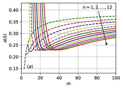
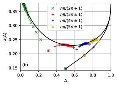
Figure 1: (a) For each fixed $n$, the function $a(\Delta)=a(\cos(n\pi/m))$ is smooth. (b) When ordered by anisotropy $\Delta$, however, the prefactor $a(\Delta)$ is fractal. Here the upper solid line denotes the envelope function obtained from the result (VI) for $\bar{\mu}>1$ in the formal limit $m\to\infty$ with $K$ fixed. The lower solid line is the result (VI) for $\bar{\mu}=1$ analytically continued for $K\leq 3/2$ ($\Delta\geq 1/2$).

In Fig. 1, the prefactor $a(\Delta)$ is plotted for various fixed $n$. While each curve for a given $n$ is a smooth function of $m$, the dependence on anisotropy $\Delta=\cos(\gamma)$ is clearly fractal. Our results thus provide further evidence that $D(\Delta)$ is analytic in $\Delta$ only for $T=0$, while it is a fractal for $T>0$.

This structure may be further analyzed by considering limiting cases of Eq. (VI). A particularly notable curiosity is the observation that for anisotropies $\gamma=\frac{n\pi}{n+1}$ $(K=n+1)$ the correction factor $a(\Delta)=0$. For other anisotropies $\gamma=\frac{n\pi}{m}$ with fixed $n$, the Drude weight correction term $a(\Delta)$ also falls onto continuous curves for fixed string length $\bar{\mu}$. Along these curves, limiting values of the Drude weight correction may be determined for anisotropies intersecting with these curves. The possible limits that can be carried out are $m\to\infty$, for fixed $n$, and $\frac{1}{p_{0}}=\frac{\gamma}{\pi}\to c$ for fixed $\bar{\mu}>1$, which are accomplished by treating the denominator $m$ as a function of the numerator $n$ such that the string length is kept fixed. We note that $\mathcal{C}$ diverges like $m$ as $\gamma\to\pi/3$ and otherwise converges to a finite constant. From the trigonometric functions in Eq. (VI) it is then obvious that $\lim_{\Delta\to\frac{1}{2}}a(\Delta)\neq a\left(\frac{1}{2}\right)$, which is what we mean when calling the Drude weight fractal. As an example, the curve with constant string length $\bar{\mu}=3$ approaching $\gamma=\pi/3$ clearly demonstrates this fractal property as can be seen in Fig. 2.

Figure 2: Prefactor $a(\Delta)$ for constant string length $\bar{\mu}=3$ approaching $\gamma=\frac{\pi}{3}$. There is a clear jump at $\gamma=\frac{\pi}{3}$ which exemplifies the fractal character of the Drude weight at low temperatures.

We note that the prefactor $a(\Delta)$ in Eq. (VI) is always finite. There are no divergencies. Furthermore, we note that our analytical low-temperature asymptotics do not apply at the isotropic point $\Delta=1$ ($K=1$). Here the ordering of the temperature corrections collapses: terms such as $T^{r(4K-4)}$ with $r$ integer which are next-leading for $K>1$ all show the same temperature scaling as the $T^{2K-2}$ term in the limit $K\to 1$. A numerical evaluation of Zotos’ formula for $m\to\infty$ indicates that $D(T>0)=0$ at the isotropic point, which is consistent with the quasilocal charges becoming non-local for $\Delta\to 1$ [9, 31, 32]. This vanishing of the Drude weight at the isotropic point has been used to argue in support of superdiffusive transport at $\Delta=1$ [30, 46].

VII Integer exponents and numerical results

So far, we have concentrated on the pole of the kernel $\omega(\theta)$ leading to the $T^{2K-2}$ temperature correction. In addition, there are poles which are independent of anisotropy and lead to temperature corrections $T^{2r}$ with $r\in\mathbb{N}$ as well as higher order corrections $\sim T^{r(2K-2)}$, $r=2,3,\cdots$. In principle, one could try to extend the asymptotic analysis of the TBA equations discussed in the previous sections to obtain results beyond the $T^{2K-2}$ temperature correction. Having seen how technically demanding it is to obtain just the $T^{2K-2}$ asymptotics, we will however instead argue that other corrections—in particular the $T^{2}$ correction which is dominant for $-1<\Delta\leq 0$—can be obtained in a standard field theoretical calculation and are, in fact, already known, see Refs. [8, 7].

We start by numerically studying the next-leading temperature corrections in the two regimes $0<\Delta<1/2$ and $1/2<\Delta<1$. As shown in Fig. 3, a power law in temperature can be clearly identified with an exponent which is different in the two regimes.

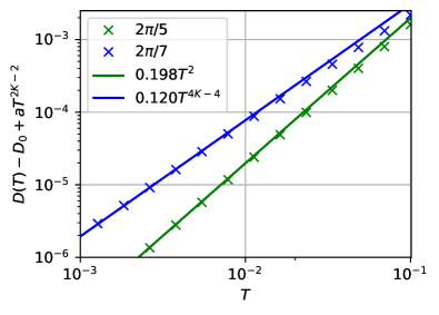
Figure 3: Numerical results for $D(T)$ based on Eq. (8) with the zero-temperature Drude weight $D(0)$ and the leading temperature correction $aT^{2K-2}$ subtracted for $\Delta=\cos(2\pi/5)\approx 0.31$ and $\Delta=\cos(2\pi/7)\approx 0.62$. For $\gamma=2\pi/5$ the next-leading correction scales as $T^{2}$ while it scales as $T^{4K-4}$ with $K=7/5$ for $\gamma=2\pi/7$.

In a field theoretical description of the XXZ chain, we obtain the standard free boson theory in the scaling limit with perturbations stemming from band curvature and from Umklapp scattering. From the scaling dimensions of these operators, we expect that band curvature leads to temperature-dependent corrections of the Drude weight $\sim T^{2r}$, with $r$ a positive integer, while Umklapp scattering results in terms scaling as $T^{r(2K-2)}$. The numerical findings in Fig. 3 are in agreement with these expectations. For $0<\Delta<1/2$ ($3/2<K<2$) the next-leading correction scales as $T^{2}$ while the temperature dependence changes to $T^{4K-4}$ for $1/2<\Delta<1$ ($1<K<3/2$).

In Refs. [8, 7], a standard bosonization approach was used to calculate the spin conductivity $\sigma(q,\omega)$ as a function of momentum $q$ and frequency $\omega$. Band curvature and Umklapp scattering were taken into account by a perturbative calculation of the retarded self-energy $\Pi^{\textrm{ret}}(q,\omega)$ leading to

$$\Pi^{\textrm{ret}}(q,\omega)\approx-2\mathrm{i}\gamma\omega+b\omega^{2}+cv_{0}^{2}q^{2}\,.$$ (54)

The problem with this result is that the imaginary part of the self-energy, characterized by the relaxation rate $\gamma$, will lead to a complete decay of the current-current correlation function $\langle J_{0}(t)J_{0}(0)\rangle/N\sim\exp(-2\gamma t)$; there is no Drude weight. The reason is that the integrable structure of the microscopic model—in particular, the existence of quasi-local conserved charges—is not reflected in the standard field theoretical approach. We want to argue here that this issue only affects the imaginary part of the self energy and that the real part is not affected by the quasi-local charges and does contain information about other temperature corrections to the Drude weight. In particular, perturbations of the free boson model due to band curvature do not relax the current—independent of whether or not local conservation laws exist—and can be treated in a standard perturbative manner. Setting the relaxation rate $\gamma=0$—which would correspond to purely ballistic transport—the Drude weight in this field theory approach is given by (see Eq. (2.52) in Ref. [8])

$$D(T)=\frac{Kv_{0}}{4\pi(1+b(T))}$$ (55)

with

$$b=(Y_{2}-Y_{3})T^{4K-4}+Y_{4}T^{2}\,.$$ (56)

Here the $T^{4K-4}$ term is obtained in second order perturbation theory in Umklapp scattering while the $T^{2}$ term is obtained in first order in band curvature. Due to the integrability of the model, the amplitudes $Y_{2},\,Y_{3}$, and $Y_{4}$—which are functions of $K$, $v_{0}$ only—can be determined. They are given in Ref. [8] and we will reproduce them for convenience in App. D. The hypothesis that (56) contains parts of the additional temperature corrections to the Drude weight is supported by a comparison of Eq. (55) with the Bethe ansatz calculations based on spinons and anti-spinons in Ref. [13]. The latter approach also appears to assume that spin transport is purely ballistic at all temperatures. The results of the two approaches at low temperatures are in excellent agreement, see Fig. 2 in Ref. [8].

The partial decay of the Drude weight is caused by Umklapp scattering which turns two right movers into left movers and vice versa and is therefore able to relax the part of the current which is not protected by the quasi-local conserved charges. While the proper field theoretical treatment of the quasi-local charges is not yet known, the scaling dimension and the prefactor of the leading temperature correction in Eq. (VI) show that this term corresponds to a correction which is first order in Umklapp scattering. In second order in Umklapp scattering, which leads to a $T^{4K-4}$ temperature correction, there are two contributions: a contribution which does not change the current and is contained in Eqs. (55,56), and a contribution which does change the current and which we have not determined here.

We therefore conjecture that the Drude weight of the XXZ chain for $-1<\Delta<1$ at low temperatures is asymptotically given by

$$D(T)=D_{0}-aT^{2K-2}-b_{1}T^{2}-b_{2}T^{4K-4}$$ (57)

with $D_{0}=Kv_{0}/4\pi$ and $a$ being the prefactor in Eq. (VI) which does depend, in general, on $m$ and $K$. Here we have defined $b_{1}=D_{0}Y_{4}$ and $b_{2}=D_{0}(Y_{2}-Y_{3}+c)$ where $Y_{2},\,Y_{3},\,Y_{4}$ are the amplitudes given in Eq. (D). The term $\sim cT^{4K-4}$ is the current relaxing contribution which we expect to occur in second order in Umklapp scattering with an unknown amplitude $c$. The amplitude $Y_{4}$ diverges whenever the exponent of one of the higher order Umklapp contributions becomes equal to $2$, i.e. when $r(4K-4)=2$ which is equivalent to $K=(2r+1)/(2r)$. These divergencies have to be cancelled by the amplitudes of those parts of the higher Umklapp terms which are not current relaxing. We will show this explicitly for $K=3/2$ below. For the amplitude $c$ of the current relaxing part, on the other hand, we expect no divergencies but—similar to the $T^{2K-2}$ term—a fractal dependence on $n,m$. Although we do not know the amplitude of the $T^{4K-4}$ temperature correction completely, we keep the known part because the divergence of $Y_{4}$ would otherwise make the formula (57) unusable for $K\sim 3/2$ ($\Delta\sim 1/2$). We stress again that the $T^{2}$ term is the dominant temperature correction for $-1<\Delta\leq 0$ and including this term is thus essential to obtain an asymptotic result which is valid in the entire regime $-1<\Delta<1$.

Our hypothesis (57) can be checked directly for the free fermion point $\Delta=0$. Here the current operator $J_{0}$ is conserved and the Drude weight is simply given by a static expectation value

$$D=\frac{\langle J_{0}^{2}\rangle}{2NT}=\frac{1}{8\pi T}\int_{-\pi}^{\pi}\frac{\sin^{2}(k)\,dk}{\cosh\left(\frac{\varepsilon_{k}}{T}\right)+1}$$ (58)

with $\varepsilon_{k}=-\cos k$. The leading temperature dependence can be obtained by an asymptotic evaluation of the integral and one finds

$$D(T)=\frac{1}{2\pi}-\frac{\pi}{12}T^{2}-\frac{7\pi^{3}}{240}T^{4}-\mathcal{O}(T^{6})\,.$$ (59)

In Eq. (57), the amplitudes $a$ and $Y_{2}-Y_{3}$ vanish for $\Delta=0$ as can be checked explicitly but is also obvious because Umklapp scattering, which is responsible for the temperature corrections with non-integer exponents, is not present at the free fermion point. Finally, $b_{1}\to\pi/12$ for $\Delta\to 0$ showing that the leading temperature corrections are consistent with the free fermion result. We therefore expect that $D(T)$ near the free fermion point is described over a fairly large temperature range by Eq. (57). This is indeed the case, see Fig. 4.

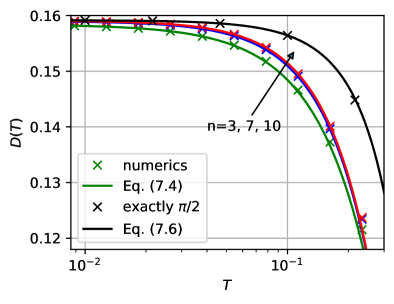
Figure 4: Numerical results for $D(T)$ compared to the analytical result (59) at the free fermion point and the asymptotics (57) for anisotropies near the free fermion point, $\gamma=n\pi/(2n+1)$. The asymptotics (57) works well for temperatures $T\lesssim 0.2$.

Note that keeping only the leading $T^{2K-2}$ term, in contrast, describes the data for $0<\Delta\ll 1$ well only at extremely low temperatures.

Let us now also check the regime $-1<\Delta\leq 0$ where the $T^{2}$ term is the leading temperature correction. For $-1/2<\Delta<0$ the $T^{2K-2}$ term is next-leading while a $T^{4}$ term will be next-leading for $-1<\Delta<-1/2$. As shown in Fig. 5, Eq. (57) is consistent with the numerical data for the Drude weight at anisotropies $\gamma=n\pi/(2n-1)$ with the next-leading $T^{2K-2}$ correction being important to describe the data well up to temperatures $T\lesssim 0.1$.

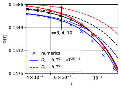
Figure 5: Numerical results for $D(T)$ at $\gamma=n\pi/(2n-1)$ with $n=3,4,10$ compared to the analytical result (57) with and without the next-leading $T^{2K-2}$ term.

The fractal structure of the Drude weight at finite temperatures is very pronounced near the free fermion point. Right at the free fermion point we have found the low-temperature asymptotics (59). Approaching the free fermion point by anisotropies $\gamma=n\pi/(2n+1)$ with $n\to\infty$, on the other hand, we find that the prefactor $a$ in Eq. (57) does not vanish but rather takes the limiting value $a\to\pi^{2}/24$. The leading temperature dependence is therefore given by

$$\lim_{n\to\infty}D_{\gamma=n\pi/(2n+1)}(T)=\frac{1}{2\pi}-\left(\frac{\pi^{2}}{24}+\frac{\pi}{12}\right)T^{2}+\mathcal{O}(T^{4})$$ (60)

in contrast to the result right at the free fermion point, Eq. (59).

Next, we consider the special case $\Delta=1/2$ ($K=3/2$). At this point, both the next-leading contribution from Umklapp scattering and the band curvature term scale as $T^{2}$ and both have divergent amplitudes. These divergencies, however, cancel and Eq. (57) yields

$$D {}_{\gamma=\pi/3}(T)=\frac{9\sqrt{3}}{32\pi}-\frac{3\pi}{64}T+\frac{1}{12\sqrt{3}\pi}T^{2}\ln T+cT^{2}$$ (61)

$$- \frac{142+24\tilde{\gamma}+48\ln 2+60\ln 3-21\zeta(3)}{288\sqrt{3}\pi}T^{2}\,.$$

which includes the current relaxing second order Umklapp contribution with unknown amplitude $c$. As shown in Fig. 6, this result without the $cT^{2}$ term is in good agreement with the numerical data.

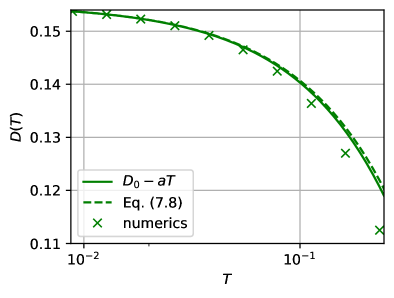
Figure 6: Numerical results for $D(T)$ at $\Delta=1/2$ compared to the analytical result (57) with and without the known part of the next-leading term.

We note that in contrast to anisotropies near the free fermion point, keeping the known parts of the next-leading terms does not increase the temperature range over which the asymptotics agrees well with the numerical results. We want to stress again, however, that by keeping the known part of the $T^{4K-4}$ correction, the result (57) is not plagued by divergencies for anisotropies $0\leq\Delta\leq 1/2$ either.

Finally, we consider anisotropies when approaching other simple roots of unity. For the approach towards $\gamma=\pi/4$ shown in Fig. 7, the leading temperature correction describes the data well in the shown temperature regime.

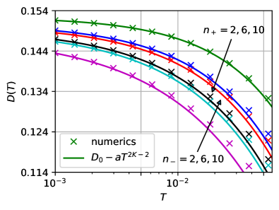
Figure 7: Numerical results for $D(T)$ compared to the leading terms in the asymptotics for anisotropies $\gamma=n_{+}\pi/(4n_{+}+1)$ (circles and solid lines) and $\gamma=n_{-}\pi/(4n_{-}-1)$.

Generally speaking, the derived asymptotics holds over a smaller and smaller low-temperature range the closer we get to the isotropic point. This is a consequence of all the different temperature corrections $T^{r(2K-2)}$ with $r\in\mathbb{N}$ collapsing for $K\to 1$. Directly at the isotropic point, our result is not applicable.

VIII Conclusions

We have obtained an analytic result for the leading low-temperature asymptotics of the Drude weight of the XXZ chain at anisotropies $\Delta=\cos(\pi n/m)$. Previously, analytical results were only known at zero and infinite temperatures. Similar to the infinite temperature case, we find that the leading low-temperature correction for $0<\Delta<1$ is a fractal as a function of anisotropy $\Delta$. From a more technical perspective, the temperature dependence of the Drude weight at low temperatures in this regime is a consequence of the combined small rapidity behavior of the effective velocity and the Fermi weight. Our analytical result agrees with numerical evaluations of Zotos’ formula and adding the $T^{2}$ correction known from a field theory approach yields a good description of the Drude weight over a finite low-temperature range for the entire regime $-1<\Delta<1$. The exception is the isotropic limit, $\Delta\to 1$, where this range shrinks to zero.

While the result for the simple roots of unity $\gamma=\pi/m$ can be expressed entirely by the Luttinger parameter $K$ and the spin velocity $v_{0}$, this is not the case for general anisotropies $\gamma=\pi n/m$. In the latter case, the $T^{2K-2}$ Drude weight correction contains a factor $m\sin(\pi K/m)$ which is responsible for the fractal structure. This puts the latter result outside the usual Luttinger liquid framework. How such a factor can emerge in a field theoretical description of this integrable lattice model remains an open question.

Appendix A Takahashi-Suzuki Integers

The Takahashi-Suzuki (TS) integers are described by a set of recursive relations that categorize the Bethe strings by their length ($\mu_{j}$), parity ($v_{j}$), and the sign of the dressed energy ($\sigma_{j}$). Continued fractions of the anisotropy are given by $\pi/\gamma=[\nu_{1},\dots,\nu_{\alpha}]$. With

$$[\nu_{1},\nu_{2},\nu_{3},\dots]=\nu_{1}+\frac{1}{\nu_{2}+\frac{1}{\nu_{3}+\dots}}$$ (62)

these give rise to the $m$-integers

$$m_{j}=\sum_{\ell=1}^{j}\nu_{\ell}.$$ (63)

The $\nu_{i}$ integers that appear in the continued fractions yield relations for TS-integers

$$y_{j}=y_{j-2}+\nu_{j}y_{j-1},\,\,1\leq j\leq\alpha,$$

$$y_{-1}=0,\,y_{0}=1,\,y_{1}=\nu_{1}\,,$$ (64)

as well as for the $p$-numbers

$$p_{j}=p_{j-2}-\nu_{j-1}p_{j-1},\,\text{ for }2\leq j\leq\alpha+1,$$ (65)

$$p_{0}=\frac{\pi}{\gamma},\,p_{1}=1,\,\text{ and }p_{\alpha+1}=0.$$

With the above numbers, the string lengths are then determined by

$$\mu_{j}=y_{\ell-1}+(j-m_{\ell})y_{\ell},\,\text{ for }\,m_{\ell}\leq j<m_{\ell+1},$$

$$m=y_{\alpha}=\mu_{m_{\alpha}-1}+\mu_{m_{\alpha}}.$$ (66)

The string parity is characterized by

$$z_{j}=z_{j-2}+\nu_{j}z_{j-1},\,\text{ for }\,1\leq j\leq\alpha$$

$$z_{-1}=1,\,z_{0}=0,\,z_{1}=1.$$ (67)

The parity is given in terms of the string length and anisotropy $\gamma=\frac{\pi n}{m}$ as

$$v_{j} = (-1)^{\left\lfloor\frac{{(\mu_{j}-1)n}}{m}\right\rfloor},\text{ if }j\neq m_{1},$$

$$v_{m_{1}} = -1.$$ (68)

Finally, the numbers $q_{j}$ are given by

$$q_{j} = (p_{i}-(j-m_{i})p_{i+1})(-1)^{i},\,\,\text{ for }m_{i}\leq j<m_{i+1},$$

$$q_{m_{\alpha}} = -q_{m_{\alpha}-1},$$ (69)

which can be used to determine $\sigma_{j}=\text{sign}(q_{j})$.

Appendix B Largest Eigenvalue

The largest eigenvalue may be written in terms of the auxiliary functions by using a method analogous to the one used to derive (27) and the non-linear integral relations themselves. In order to be consistent with earlier definitions, the Fourier transformation (FT) is defined as $f(k)=\int d\theta\text{e}^{-\mathrm{i}k\theta}f(\theta)$. The largest eigenvalue of the quantum transfer matrix is related to the auxiliary functions as

$$\Lambda = \frac{q^{2\mathrm{i}}\phi^{-\mathrm{i}}}{q}+\frac{q^{-2\mathrm{i}}\phi^{\mathrm{i}}}{q},$$

$$\Lambda^{\mathrm{i}} = \frac{q^{-\mathrm{i}}\phi^{2\mathrm{i}}}{q^{\mathrm{i}}}\left(1+\frac{q^{3\mathrm{i}}\phi}{q^{-\mathrm{i}}\phi^{2\mathrm{i}}}\right)=\frac{q^{-\mathrm{i}}\phi^{2\mathrm{i}}}{q^{\mathrm{i}}}A,$$

$$\Lambda^{-\mathrm{i}} = \frac{q^{\mathrm{i}}\phi^{-2\mathrm{i}}}{q^{-\mathrm{i}}}\left(1+\frac{q^{-3\mathrm{i}}\phi}{q^{\mathrm{i}}\phi^{-2\mathrm{i}}}\right)=\frac{q^{\mathrm{i}}\phi^{-2\mathrm{i}}}{q^{-\mathrm{i}}}\bar{A}.$$ (70)

We define $f_{k}=FT(\partial_{\theta}\ln(f))$ which, taken together with the definition of the Fourier transform, implies that $f(\theta+\mathrm{i}h)=f^{\mathrm{i}h}\to\text{e}^{-kh}f_{k}$ provided that the shifted contour lies in the same analyticity strip, i.e. $\Im(\theta+\mathrm{i}h)\in(0,2p_{0})$. This is our fundamental domain for $q$ and $\phi$. The $q$ and $\phi$ functions are related back to the auxiliary functions by taking the difference of the two Fourier transformed eigenvalues

$$0 = -q_{k}\text{e}^{-p_{0}k}\left(\text{e}^{k}+\text{e}^{-k}\right)\left(\text{e}^{(p_{0}-1)k}-\text{e}^{(1-p_{0})k}\right)$$

$$+ \phi_{k}\text{e}^{-p_{0}k}\left(\text{e}^{(p_{0}-1)k}-\text{e}^{(1-p_{0})k}\right)+A\text{e}^{k}-\bar{A}_{k}\text{e}^{-k},$$

$$q_{k} = \frac{\phi_{k}}{e^{k}+\text{e}^{-k}}+\frac{\text{e}^{p_{0}k}\left(A_{k}\text{e}^{k}-\bar{A}_{k}\text{e}^{-k}\right)}{\left(\text{e}^{k}+\text{e}^{-k}\right)\left(\text{e}^{(p_{0}-1)k}-\text{e}^{(1-p_{0})k}\right)}.$$ (71)

By adding the terms together instead, the largest eigenvalue can likewise be determined in terms of the auxiliary functions as

$$\Lambda_{k} = \phi_{k}\text{e}^{-p_{0}k}\frac{\text{e}^{(2-p_{0})k}+\text{e}^{(p_{0}-2)k}}{e^{k}+e^{-k}}+\frac{A_{k}+\bar{A}_{k}}{\text{e}^{k}+\text{e}^{-k}}\,.$$ (72)

The largest eigenvalue is related to the free energy, whereas (71) is another form of Eq. (27) that is used to determine the Fermi weight for the simple roots of unity. By carrying out the inverse Fourier transform and integrating Eq. (71) the relation is explicitly obtained

$$\ln\frac{\phi^{\mathrm{i}p_{0}}}{q^{\mathrm{i}(p_{0}+1)}q^{\mathrm{i}(p_{0}-1)}}=\left[\omega^{\mathrm{i}}\star\ln\bar{A}-\omega^{-\mathrm{i}}\star\ln A\right].$$ (73)

These relations also allow to expand $\frac{\Lambda}{q^{2\mathrm{i}}q^{-2\mathrm{i}}}$ into

$$\Lambda_{k}-q_{k}\left(\text{e}^{-2k}+\text{e}^{(2-2p_{0})k}\right) = \frac{\text{e}^{(p_{0}-2)k}\bar{A}_{k}-\text{e}^{(2-p_{0})k}A_{k}}{\text{e}^{(p_{0}-1)k}-\text{e}^{(1-p_{0})k}}.$$

This results in the identity used for the eigenvalue trick from the main body of the paper

$$\ln\frac{\Lambda}{q^{2\mathrm{i}}q^{-2\mathrm{i}}}=\left[\omega^{\mathrm{i}(2-p_{0})}\star\ln\bar{A}-\omega^{\mathrm{i}(p_{0}-2)}\star\ln A\right].$$ (75)

Appendix C Proof of Eq. (25)

This proof uses the notation of Ref. [44] for the Takahashi Suzuki (TS) integers and the shorthand for imaginary shifts $f(\theta+ic)=f^{\mathrm{i}c}$. Eq. (25) comes from the identification of the particle/hole density of the second to last string with $K(\theta)$ appearing in the $Y$-system. This identification appears in the fusion hierarchy of the the easy-plane ($|\Delta|\leq 1$) regime of the XXZ for rational anisotropies $\gamma$, where $\Delta=\cos(\gamma)$. This section will deal with the $L-1$-th string again, $\eta(\theta)\equiv\eta_{L-1}(\theta)$, which is related back to the transfer matrices by

$$\eta=K(\theta)=\frac{T_{\mu-1}^{\mathrm{i}(z_{\alpha}-z_{\alpha-1}-1)p_{0}}}{T_{\bar{\mu}-1}^{\mathrm{i}(y_{\alpha}+(z_{\alpha}-z_{\alpha-1}-1)p_{0})}}.$$ (76)

The transfer matrices $T_{r-1}(\theta)$ are defined as

$$T_{r-1}=q^{\mathrm{i}r}q^{-\mathrm{i}r}\sum_{j=1}^{r}\frac{\phi^{\mathrm{i}(2j-r-1)}}{q^{\mathrm{i}(2j-r)}q^{\mathrm{i}(2j-r-2)}}\,.$$ (77)

Here the notation deviates slightly from [44] with $\phi(\theta)=\left(\sinh\left[\frac{\gamma(\theta+\mathrm{i}u+\mathrm{i})}{2}\right]\sinh\left[\frac{\gamma(\theta-\mathrm{i}u-\mathrm{i})}{2}\right]\right)^{N/2}$, where $N$ is the Trotter number, and the variable $u=-\frac{J\sin{\gamma}}{T\gamma N}$. The shifts that occur in the transfer matrices are fixed by the anisotropy through the relation

$$z_{\alpha-1}p_{0}=y_{\alpha-1}+(-1)^{\alpha}p_{\alpha}=\bar{\mu}+\frac{(-1)^{\alpha}}{n}.$$ (78)

The equality follows from $y_{\alpha-1}=\bar{\mu}$ and $p_{\alpha}=1/n$ for an anisotropy $\pi/\gamma=m/n=[\nu_{1},\dots,\nu_{\alpha}]$ , the latter is also used and proven in [37]. A second straightforward, but useful equality is that $z_{\alpha}=n$, so $p_{0}z_{\alpha}=y_{\alpha}=m$. With these identifications made, the quantity $\eta+1$ is noted to be the inverse of the Fermi weight for what we refer to as the spin-particle string, with the $L$-th string being the spin-hole string. The Fermi weight of the particle string is given by

$$\eta+1=\left(\frac{T_{\mu-1}^{\mathrm{i}(-\bar{\mu}+(-1)^{\alpha+1}/n-p_{0}+m)}}{T_{\bar{\mu}-1}^{\mathrm{i}(m-\bar{\mu}+(-1)^{\alpha+1}/n-p_{0}+m)}}+1\right).$$ (79)

For rational values of $\gamma/\pi$ we have

$$T_{y_{\alpha}+y_{\alpha-1}-1}=T_{y_{\alpha}-y_{\alpha-1}-1}+2T_{y_{\alpha-1}-1}^{\mathrm{i}y_{\alpha}}.$$ (80)

For brevity of notation, we set $\widetilde{w}:=-\bar{\mu}+(-1)^{\alpha+1}/n-p_{0}+m$, which can be written as

$$\widetilde{w}=s-m+\bar{\mu}+1\,.$$ (81)

with $s$ given in Eq. (26).

Applying Eq. (80), the inverse Fermi weight may then be written as

$$\eta+1=\left(\frac{T^{\mathrm{i}\widetilde{w}}_{m+\bar{\mu}-1}-T^{\mathrm{i}(\widetilde{w}+m)}_{\bar{\mu}-1}}{T^{\mathrm{i}(m+\widetilde{w})}_{\bar{\mu}-1}}\right).$$ (82)

Further simplification requires some additional information on the sum appearing in the definition of the transfer matrix. It is known that $T_{r-1}^{2m\mathrm{i}}=T_{r-1}$, which follows from the cyclicity of the $\phi$, $q$ functions. This cyclic relation permits us to conclude that the following sum is a constant

$$\sum_{j=1}^{m}\frac{\phi^{\mathrm{i}(2j-1-m)}}{q^{\mathrm{i}(2j-m)}q^{\mathrm{i}(2j-2-m)}}=m.$$ (83)

The reason is that all poles of the terms in the sum cancel pairwise, they have finite asymptotics, hence the sum is bounded. Due to Liouville’s theorem the sum is constant. The constant value is identical to the limiting value $m$.

Consequently, the transfer matrices in the numerator of (82) are expanded as

$$T_{m+\bar{\mu}-1}^{\mathrm{i}\widetilde{w}} = q^{\mathrm{i}(m+\bar{\mu}+\widetilde{w})}q^{-\mathrm{i}(m+\bar{\mu}-\widetilde{w})}$$

$$\!\!\!\!\!\times \!\!\!\!\!\left(\sum_{j=m+1}^{\bar{\mu}+m}\frac{\phi^{\mathrm{i}(2j-1-m-\bar{\mu}+\widetilde{w})}}{{q^{\mathrm{i}(2j-m-\bar{\mu}+\widetilde{w})}q^{\mathrm{i}(2j-2-m-\bar{\mu}+\widetilde{w})}}}+m\right),$$

$$T_{\bar{\mu}-1}^{\mathrm{i}(\widetilde{w}+m)} = q^{\mathrm{i}(\bar{\mu}+\widetilde{w}+m)}q^{-\mathrm{i}(\bar{\mu}-\widetilde{w}-m)}$$ (84)

$$\times \sum_{j=1}^{\bar{\mu}}\frac{\phi^{\mathrm{i}(2j-1+m-\bar{\mu}+\widetilde{w})}}{{q^{\mathrm{i}(2j+m-\bar{\mu}+\widetilde{w})}q^{\mathrm{i}(2j-2+m-\bar{\mu}+\widetilde{w})}}}.$$

The difference is evaluated by noting that shifts by $2m$ leave the result unchanged. In the first line $j\to j+m$ is taken, which results in the same sum as in the second line. Thus the numerator of the inverse Fermi weight (82) is

$$T_{m+\bar{\mu}-1}^{\mathrm{i}\widetilde{w}}-T_{\bar{\mu}-1}^{\mathrm{i}(\widetilde{w}+m)}=q^{\mathrm{i}(m+\bar{\mu}+\widetilde{w})}q^{-\mathrm{i}(m+\bar{\mu}-\widetilde{w})}m.$$ (85)

By expanding all transfer matrices we obtain

$$\eta+1={m}\left[{\sum_{j=1}^{\bar{\mu}}\frac{\phi^{\mathrm{i}(2j-1+m-\bar{\mu}+\widetilde{w})}}{{q^{\mathrm{i}(2j+m-\bar{\mu}+\widetilde{w})}q^{\mathrm{i}(2j-2+m-\bar{\mu}+\widetilde{w})}}}}\right]^{-1},$$ (86)

or in terms of the particle Fermi weight $\vartheta(\theta)=\frac{1}{\eta(\theta)+1}$

$$\vartheta=\frac{1}{m}\sum_{j=1}^{\bar{\mu}}\frac{\phi^{\mathrm{i}(2j-1+m-\bar{\mu}+\widetilde{w})}}{{q^{\mathrm{i}(2j+m-\bar{\mu}+\widetilde{w})}q^{\mathrm{i}(2j-2+m-\bar{\mu}+\widetilde{w})}}}.$$ (87)

This is exactly the relation (25) in the main text.

Appendix D Amplitudes of next-leading corrections

For completeness, we reproduce here the amplitudes $Y_{2}$, $Y_{3}$, $Y_{4}$ of the $T^{2}$ and $T^{4K-4}$ temperature corrections in Eq. (56) from Ref. [48].

The bosonized Hamiltonian of the XXZ chain is given by

$$H = H_{0}+H_{u}+H_{bc},\quad H_{0}=\frac{v_{0}}{2}\int dx\,[\Pi^{2}+(\partial_{x}\varphi)^{2}]$$

$$H_{u} = \lambda\int dx\,\cos(\sqrt{8\pi K}\varphi)]$$ (88)

$$H_{bc} = -2\pi v_{0}\lambda_{+}\int dx\,(\partial_{x}\varphi_{R})^{2}(\partial_{x}\varphi_{L})^{2}$$

$$-2\pi v_{0}\lambda_{-}\int dx\,[(\partial_{x}\varphi_{R})^{4}+(\partial_{x}\varphi_{L})^{4}]$$

where $H_{0}$ is the standard Luttinger liquid Hamiltonian, $H_{u}$ the Umklapp term, and $H_{bc}$ the band curvature terms. The amplitudes have been determined exactly by a comparison with Bethe ansatz results [49]

$$\lambda = \frac{K\Gamma(K)\sin(\pi/K)}{\pi\Gamma(2-K)}\left[\frac{\Gamma\left(1+\frac{1}{2K-2}\right)}{2\sqrt{\pi}\Gamma\left(1+\frac{K}{2K-2}\right)}\right]^{2K-2},$$

$$\lambda_{+} = \frac{1}{2\pi}\tan\frac{\pi K}{2K-2},$$ (89)

$$\lambda_{-} = \frac{1}{12\pi K}\frac{\Gamma\left(\frac{3K}{2K-2}\right)\Gamma^{3}\left(\frac{1}{2K-2}\right)}{\Gamma\left(\frac{3}{2K-2}\right)\Gamma^{3}\left(\frac{K}{2K-2}\right)}.$$

The calculation of the self-energy in second order perturbation theory in $H_{u}$ and first order perturbation theory in $H_{bc}$ then yields the following amplitudes for the next-leading temperature corrections

$$Y_{1} = \Lambda\frac{B(K,1-2K)}{\sqrt{\pi}2^{2K+1}}\cot(\pi K),$$

$$Y_{2} = \Lambda\frac{B(K,1-2K)}{\pi^{5/2}2^{2K+4}}(\pi^{2}-2\Psi^{\prime}(K)),$$

$$Y_{3} = \Lambda\frac{1}{\pi 2^{4K+4}}\cot^{2}(\pi K)\Gamma(1/2-K)\Gamma(K),$$ (90)

$$Y_{4} = \frac{\pi^{2}}{6v^{2}}(\lambda_{+}+6\lambda_{-}),$$

$$\Lambda = 4\pi K\lambda^{2}\sin(2\pi K)\left(\frac{2\pi}{v}\right)^{4K-2}\Gamma(1/2-K)\Gamma(K),$$

with $B(x,y)$ being the Beta function and $\Psi(x)$ being the Digamma function.

References

- Shastry and Sutherland [1990] B. S. Shastry and B. Sutherland, Twisted boundary conditions and effective mass in Heisenberg-Ising and Hubbard rings, Physical Review Letters 65, 243 (1990).
- Zotos et al. [1997] X. Zotos, F. Naef, and P. Prelovsek, Transport and conservation laws, Physical Review B 55, 11029 (1997).
- Castella et al. [1995] H. Castella, X. Zotos, and P. Prelovsek, Integrability and ideal conductance at finite temperatures, Physical Review Letters 74, 972 (1995).
- Zotos [1999] X. Zotos, Finite temperature Drude weight of the one dimensional spin 1/2 Heisenbeg, Physical Review Letters 82, 1764 (1999).
- Sakai and Klümper [2003] K. Sakai and A. Klümper, Non-dissipative thermal transport in the massive regimes of the XXZ chain, Journal of Physics A: Mathematical and General 36, 11617 (2003).
- Klümper and Sakai [2002] A. Klümper and K. Sakai, The thermal conductivity of the spin-1/2 XXZ chain at arbitrary temperature, Journal of Physics A: Mathematical and General 35, 2173 (2002).
- Sirker et al. [2009] J. Sirker, R. G. Pereira, and I. Affleck, Diffusion and ballistic transport in one-dimensional quantum systems, Physical Review Letters 103, 10.1103/PhysRevLett.103.216602 (2009).
- Sirker et al. [2011] J. Sirker, R. G. Pereira, and I. Affleck, Conservation laws, integrability and transport in one-dimensional quantum systems, Physical Review B 83, 10.1103/PhysRevB.83.035115 (2011).
- Prosen [2011] T. Prosen, Exact nonequilibrium steady state of a strongly driven open XXZ chain, Physical Review Letters 107, 10.1103/PhysRevLett.107.137201 (2011).
- Kinoshita et al. [2006] T. Kinoshita, T. Wenger, and D. S. Weiss, A quantum Newton’s cradle, Nature 440, 900 (2006).
- Zvyagin [1991] A. Zvyagin, Momentum oscillation in degenerated Hubbard chain, Sov. J. Low Temp. Phys. 17, 779 (1991).
- Boos et al. [2006] H. E. Boos, F. Göhmann, A. Klümper, and J. Suzuki, Factorization of multiple integrals representing the density matrix of a finite segment of the Heisenbeg spin chain, Journal of Statistical Mechanics: Theory and Experiment 2006, P04001 (2006).
- Benz et al. [2005] J. Benz, T. Fukui, A. Klümper, and C. Scheeren, On the finite temperature Drude weight of the anisotropic Heisenbeg chain, Journal of the Physical Society of Japan 74, 181 (2005).
- Aufgebauer et al. [2010] B. Aufgebauer, M. Brockmann, W. Nuding, A. Klümper, and A. Sedrakyan, The complete conformal spectrum of a sl(2|1) invariant network model and logarithmic corrections, Journal of Statistical Mechanics Theory and Experiment 2010, 10.1088/1742-5468/2010/12/P12010 (2010).
- Göhmann [2020] F. Göhmann, Statistical mechanics of integrable quantum spin systems, SciPost Phys. Lect. Notes , 16 (2020).
- Göhmann et al. [2019] F. Göhmann, K. K. Kozlowski, J. Sirker, and J. Suzuki, Equilibrium dynamics of the XX chain, Phys. Rev. B 100, 155428 (2019).
- Babenko et al. [2020] C. Babenko, F. Göhmann, K. K. Kozlowski, J. Sirker, and J. Suzuki, Exact real-time longitudinal correlation functions of the massive XXZ chain, arXiv:2012.07378 (2020).
- Castro-Alvaredo et al. [2016] O. A. Castro-Alvaredo, B. Doyon, and T. Yoshimura, Emergent hydrodynamics in integrable quantum systems out of equilibrium, Physical Review X 6, 041065 (2016).
- Bertini et al. [2016] B. Bertini, M. Collura, J. De Nardis, and M. Fagotti, Transport in out-of-equilibrium XXZ chains: Exact profiles of charges and currents, Physical Review Letters 117, 10.1103/PhysRevLett.117.207201 (2016).
- Doyon and Spohn [2017] B. Doyon and H. Spohn, Drude weight for the Lieb-Liniger Bose gas, SciPost Physics 3, 039 (2017).
- Ilievski and De Nardis [2017a] E. Ilievski and J. De Nardis, Microscopic origin of ideal conductivity in integrable quantum models, Physical Review Letters 119, 020602 (2017a).
- Takahashi [1999] M. Takahashi, Thermodynamics of One-Dimensional Solvable Models (Cambridge University Press, Cambridge, 1999).
- Borsi et al. [2020] M. Borsi, B. Pozsgay, and L. Pristyák, Current operators in Bethe ansatz and generalized hydrodynamics: An exact quantum-classical correspondence, Physical Review X 10, 011054 (2020).
- Pozsgay [2020] B. Pozsgay, Current operators in integrable spin chains: lessons from long range deformations, SciPost Physics 8, 016 (2020).
- Cubero and Panfil [2020] A. C. Cubero and M. Panfil, Generalized hydrodynamics regime from the thermodynamic bootstrap program, SciPost Physics 8, 004 (2020).
- Doyon [2019] B. Doyon, Diffusion and superdiffusion from hydrodynamic projection, arXiv:1912.01551 [cond-mat, physics:math-ph] (2019).
- Ilievski and De Nardis [2017b] E. Ilievski and J. De Nardis, Ballistic transport in the one-dimensional Hubbard model: the hydrodynamic approach, Physical Review B 96, 10.1103/PhysRevB.96.081118 (2017b).
- De Nardis et al. [2018] J. De Nardis, D. Bernard, and B. Doyon, Hydrodynamic diffusion in integrable systems, Physical Review Letters 121, 160603 (2018).
- De Nardis et al. [2019] J. De Nardis, M. Medenjak, C. Karrasch, and E. Ilievski, Anomalous spin diffusion in one-dimensional antiferromagnets, Physical Review Letters 123, 6601 (2019).
- Ilievski et al. [2018] E. Ilievski, J. De Nardis, M. Medenjak, and T. Prosen, Superdiffusion in one-dimensional quantum lattice models, Physical Review Letters 121, 0602 (2018).
- Prosen and Ilievski [2013] T. Prosen and E. Ilievski, Families of quasi-local conservation laws and quantum spin transport, Physical Review Letters 111, 10.1103/PhysRevLett.111.057203 (2013).
- Pereira et al. [2014] R. G. Pereira, V. Pasquier, J. Sirker, and I. Affleck, Exactly conserved quasilocal operators for the XXZ spin chain, Journal of Statistical Mechanics: Theory and Experiment 2014, P09037 (2014).
- Zotos [2017] X. Zotos, A tba approach to thermal transport in the XXZ Heisenberg model, Journal of Statistical Mechanics: Theory and Experiment 2017, 103101 (2017).
- Mazur [1969] P. Mazur, Non-ergodicity of phase functions in certain systems, Physica 43, 533 (1969).
- Ilievski and Quinn [2019] E. Ilievski and E. Quinn, The equilibrium landscape of the Heisenbeg spin chain, SciPost Physics 7, 033 (2019).
- Kohn [1964] W. Kohn, Theory of the insulating state, Physical Review A 133, A171 (1964).
- Urichuk et al. [2019] A. Urichuk, Y. Oez, A. Klümper, and J. Sirker, The spin Drude weight of the XXZ chain and generalized hydrodynamics, SciPost Physics 6, 005 (2019).
- Sirker [2020] J. Sirker, Transport in one-dimensional integrable quantum systems, SciPost Physics (2020).
- Klümper [1998] A. Klümper, The spin-1/2 Heisenbeg chain: thermodynamics, quantum criticality and spin-Peierls exponents, The European Physical Journal B , 677 (1998).
- Kuniba et al. [2011] A. Kuniba, T. Nakanishi, and J. Suzuki, T-systems and Y-systems in integrable systems, Journal of Physics A: Mathematical and Theoretical 44, 103001 (2011).
- Klümper [1993] A. Klümper, Thermodynamics of the anisotropic spin-1/2 Heisenbeg chain and related quantum chains, Zeitschrift for Physik B Condensed Matter 91, 507 (1993).
- Destri and de Vega [1995] C. Destri and H. J. de Vega, Unified approach to thermodynamic Bethe ansatz and finite size corrections for lattice models and field theories, Nuclear Physics B 438, 10.1016/0550-3213(94)00547-R (1995).
- Lukyanov [1998] S. Lukyanov, Low energy effective Hamiltonian for the XXZ spin chain, Nuclear Physics B 522, 10.1016/S0550-3213(98)00249-1 (1998).
- Kuniba et al. [1998] A. Kuniba, K. Sakai, and J. Suzuki, Continued fraction TBA and functional relations in XXZ model at root of unity, Nuclear Physics B 525, 10.1016/S0550-3213(98)00300-9 (1998).
- Klümper and Pearce [1992] A. Klümper and P. A. Pearce, Conformal weights of RSOS lattice models and their fusion hierarchies, Physica A183, 304 (1992).
- Ljubotina et al. [2017] M. Ljubotina, M. Žnidarič, and T. Prosen, Spin diffusion from an inhomogeneous quench in an integrable system, Nature Communications 8, 16117 (2017).
- Note [1] Square brackets are used to denote continued fractions so that .
- Pereira et al. [2007] R. G. Pereira, J. Sirker, J.-S. Caux, R. Hagemans, J. M. Maillet, S. R. White, and I. Affleck, Dynamical structure factor at small q for the XXZ spin-1/2 chain, Journal of Statistical Mechanics: Theory and Experiment 2007, P08022 (2007).
- Lukyanov [1999] S. Lukyanov, Correlation amplitude for the XXZ spin chain in the disordered regime, Physical Review B 59, 11163 (1999).