Benchmarking Embedded Chain Breaking in Quantum Annealing

Abstract

Quantum annealing solves combinatorial optimization problems by finding the energetic ground states of an embedded Hamiltonian. However, quantum annealing dynamics under the embedded Hamiltonian may violate the principles of adiabatic evolution and generate excitations that correspond to errors in the computed solution. Here we empirically benchmark the probability of chain breaks and identify sweet spots for solving a suite of embedded Hamiltonians. We further correlate the physical location of chain breaks in the quantum annealing hardware with the underlying embedding technique and use these localized rates in a tailored post-processing strategies. Our results demonstrate how to use characterization of the quantum annealing hardware to tune the embedded Hamiltonian and remove computational errors.

I Introduction

Quantum annealing (QA) has emerged as a metaheuristic for unconstrained optimization using a combination of quantum and statistical mechanics farhi2000quantum . QA performs a global search for an optimal solution using quasi-adiabatic dynamics to prepare a distribution over the eigenstate of a time-dependent Hamiltonian that defines a problem of interest. Unlike the related paradigm of adiabatic quantum optimization albash2018adiabatic ; AdiabaticQuantumComputingandQuantumAnnealing , which offers promises for finding the true ground state, QA deviates from idealized pure state dynamics predicted by the adiabatic theorem due to non-adiabatic, thermal, and open system effects chancellor2017modernizing ; mishra2018finite ; marshall2019power .

Recent experimental realizations of QA, i.e., quantum annealers, are neither perfectly adiabatic nor well described by pure quantum states johnson2011quantum . In practice, evolving too quickly violates the adiabatic theorem and introduces a probability for the system to transition to an excited state farhi2000quantum , while thermal relaxation and flux noise cause the system to deviate from unitary dynamics martinis2003decoherence ; matsuura2017quantum ; novikov2018exploring ; marshall2019power . The additional physics of QA must be accounted when characterizing the accuracy and performance of this computational method mcgeoch2013experimental ; katzgraber2014glassy ; king2015benchmarking ; heim2015quantum .

As a metaheuristic, strategies for tuning QA have proven useful for demonstrating a variety of domain-specific examples of unconstrained optimization neven2008image ; king2014algorithm ; ushijima2017graph ; dridi2017prime ; venturelli2019reverse . Recent demonstrations have used the hardware controls to reduce the effects of bias noise on QA hardware mcgeoch2013experimental ; king2015benchmarking , while others have tailored the annealing schedule to incorporate non-adiabatic effects to improve upon the probability of success steiger2015heavy ; venturelli2019reverse ; marshall2019power ; pearson2019analog . However, there are limits to how well the dynamics of quantum annealers can be be controlled and these practical considerations lead to constraints on quantum computational performance king2014algorithm ; king2015benchmarking .

A leading constraint for quantum annealers is the limited connectivity between elements of the quantum register TS_Humble_2014. Programming a sparsely connected register requires embedding the logical representation of the input Hamiltonian as a physical representation that accounts for such constraints choi2011minor ; klymko2014adiabatic ; boothby2016fast ; goodrich2018optimizing ; vyskocil2019embedding . For the embedded Hamiltonian, the computed quantum state is encoded using strongly coupled spins to represent a single logical spin. For the ideal solution state, all the physical spins representing a logical spin perfectly agree in value. A chain break corresponds to a disagreement in the state of the embedded physical spins. Methods to mitigate against chain breaks include post-processing strategies to resolve disagreement in value pudenz2015quantum ; PhysRevA.92.042310 ; mishra2016performance . Yet the physics underlying chain breaks make simple post-processing methods fail in certain cases PhysRevResearch.2.023020 , and insights into the behavior of chains breaks are needed to enable better estimates of both raw and post-processed computational accuracy.

Here we investigate the behavior of chain breaks and the impact of embedding on the probability of chain breaks. We evaluate both pre-processing and post-processing strategies that affect the probability of success in finding the true ground state as well as the rate at which chain breaks occur. We use a suite of directly embedded Ising Hamiltonians derived from instances of portfolio optimization, for which the globally optimal states and baseline performance have been reported previously grant2020benchmarking . We empirically benchmark the frequency of chain breaks observed as well as the localization within the quantum hardware with respect to problem size and intra-chain coupling. We also demonstrate how post-processing methods using the localized rates of chain breaking improve the probability of success for this benchmark.

The remainder of the presentation is organized as follows. We present a summary of QA for embedded Hamiltonians including a description of embedding and post-processing methods in Sec. II. In Sec. III, we present details of the benchmark problems and methods used to study chain breaks. We present results from these benchmarks in Sec. V and final conclusions in Sec. VI

II Quantum Annealing Embedded Hamiltonians

In the pure-state representation, quantum annealing solves the problem of finding the ground state of a Hamiltonian $H_{1}$ by evolving an initial quantum state $|\Psi(0)\rangle$ under the time-dependent Schrödinger equation

$$i\hbar\frac{d}{dt}|\Psi(t)\rangle=H(t)|\Psi(t)\rangle\hskip 28.45274ptt\in[0,T]$$ (1)

with $T$ the total annealing time. Let the idealized time-dependent Hamiltonian be given by

$$H(t)=A(s(t))H_{0}+B(s(t))H_{1}$$ (2)

with $s(t)\in[0,1]$ the control schedule and $A(s)$ and $B(s)$ the time-dependent amplitudes satisfying the conditions $A(0)\gg B(0)$ and $A(1)\ll B(1)$. The initial Hamiltonian $H_{0}=-\sum_{i}^{n}\sigma_{i}^{x}$ sums over the Pauli-$X$ operators $\sigma_{i}^{x}$ representing all $n$ spins.

The $j$-th instantaneous eigenstate at time $t$ is defined by

$$H(t)|\Phi_{j}(t)\rangle=E_{j}(t)|\Phi_{j}(t)\rangle$$ (3)

where $j$ ranges from $0$ to $N-1$ and $N=2^{n}$ corresponds to the dimension of the Hilbert space. The probability of staying in the ground state throughout the anneal is high as long as the annealing times $T$ is sufficiently long. In particular, $T$ must be much greater than $O({g^{-2}_{min}})$ where $g_{min}$ is the minimum energy gap between the ground state manifold and nearest lying excited states farhi2000quantum .

We will only consider instances of $H_{1}$ represented by the (logical) Ising Hamiltonian

$$H_{1}=\sum_{i}h_{i}\sigma_{i}^{z}+\sum_{i,j}J_{i,j}\sigma_{i}^{z}\sigma_{j}^{z}+\beta$$ (4)

where $h_{i}$ is the bias on the $i^{th}$ spin, $J_{i,j}$ is the coupling strength between the $i^{th}$ and $j^{th}$ spins, $\sigma_{i}^{z}$ is the Pauli-$Z$ operator for the $i^{th}$ spin, and $\beta$ is a problem-dependent constant. This form for $H_{1}$ is well known to express many combinatorial optimization problems lucas2014ising .

For our benchmarks, we use the commercial quantum annealers available for research from D-Wave Systems johnson2011quantum . Our tests use the D-Wave 2000Q device, which represents a lattice of up to 2048 programmable superconducting flux qubits. As discussed above, many different sources contribute to non-adiabatic dynamics that cause two types of measurable errors in the logical solution. The first error is an excitation of the system in which the measured sample solution is an excited state which can be caused by Landau-Zener tunneling at level crossings between the lowest energy states or thermal excitations which cause the system to leave ground state Albash_2015 ; PhysRevA.65.012322 ; amin2009decoherence . The second error appears from thermal or magnetic noise that affects only some physical spins in the chain which causes a broken chain in the sample solution.

II.1 Embedded Hamiltonians

Consider the graphical representation of the logical Hamiltionian $G_{l}=(V_{l},E_{l})$ with vertices $V_{l}$ that represent the $n$ spins and edges $E_{l}$ that represent couplings between these spin sites. Embedding maps the logical Hamiltonian $G_{l}$ to a physical Hamiltonian $G_{p}$ as $G_{l}\rightarrow G_{p}$ by representing each vertex $v_{i}\in V_{l}$ by a subgraph, or chain, $T_{i}$. Edges within each chain $T_{i}$ specify the intra-chain coupling between physical spins, while edges between different chains specify inter-chain coupling. The embedded physical Hamiltonian is represented by the graph $G_{p}=(V_{p},E_{p})$ with vertices $V_{p}$ that correspond to physical spin sites and edges $E_{p}$ that correspond to the inter- and intra-chain couplings between these physical spins.

Embedding selects chains that satisfy the constraints of both the logical graph $G_{l}$ and the physical hardware connectivity with graph $G_{p}$. There are several methods available for embedding graphs into the physical Chimera lattice, which has $8$ qubits per unit cell with a maximum connectivity of $6$ between qubits as seen in Figure 8. A standard method of embedding is a random embedding algorithm which randomly assigns qubits in chains on the hardware such that all qubits have the necessary connection to satisfy the logical problem. A method for embedding developed by Boothby, King, and Roy based on a clique embedding which is an algorithm which is designed to embed problems with fully connected graphs by minimizing chain length and maximizing the clique which gives more symmetry. Clique embedding typically generates shorter (relative to a random embedding) and uniform chain lengths of size

$$l_{c}=\frac{n}{4}+1$$ (5)

for $n$ logical spins boothby2016fast . Theory suggests that shorter chain lengths lead to a lower probability of errors caused by noise Young_2013 ; venturelli2015quantum ; boothby2016fast .

Given an embedding with hardware graph $G^{*}=(V^{*},E^{*})$, the resulting Hamiltonian embedded is specified as

$$H^{*}=-\sum_{l\in V^{*}}h_{l}^{*}\sigma^{z}_{l}-\sum_{(l,m)\in E^{*}}J_{l,m}^{*}\sigma^{z}_{l}\sigma^{z}_{m}$$ (6)

The physical biases are given by

$$h_{l}^{*}=\frac{h_{i}}{|T_{i}|}$$ (7)

for all physical spins $l,m\in V_{T_{i}}$ where $V_{T_{i}}$ is the chain for the $i^{th}$ logical spin, and

$$J_{l,m}^{*}=\begin{cases}\frac{J_{i,j}}{\text{edges}(T_{i},T_{j})},&\text{ for }l\in T_{i},m\in T_{j},\text{and }i\neq j\\ k,&\ \text{for }l\in T_{i},m\in T_{j},\text{and }i=j\\ 0,&\ \text{otherwise}\end{cases}$$ (8)

where the parameter $k$ represents the intra-chain coupling. The value of $k$ is chosen to ensure intra-chain spins are strongly coupled relative to the magnitude of the inter-chain coupler strength, i.e., $|J_{i,j}|$ which is normalized in be in range $[0,1]$.

Ensuring an embedded chain of spins collectively represents a single logical variable requires an intra-chain coupling chain strength $k$ that is larger in magnitude than the inter-chain couplings. In other words, the chain of physical spins must be strongly coupled to remain a single logical spin. However, chains can become “broken” in so far as individual physical spins within the chain differ in their final state.

In general, chain breaks arise from nonadiabatic dynamics that lead to local excitation out of the lowest energy state with theory suggesting that longer chains are more susceptible to these effects king2014algorithm ; Dziarmaga_2005 . King et al. observed that chains break with higher probability when $k$ is too low, while errors from noise on the hardware such as from non-zero temperature and magnetic interference can be amplified if the magnitude of the intra-chain coupling $|k|$ is much greater than the inter-chain couplings $|J_{i,j}|$. These discrepancies are found to decrease the overall probability of finding the ground state king2014algorithm .

Venturelli et al. found that solution quality when solving fully connected graphs on the D-Wave $2$ (an predecessor to the D-Wave 2000Q with up to 1000 physical qubits and the same Chimera structure) varies when tuning $k$ to minimize the number of ground states returned with broken chains venturelli2015quantum . Hamerly et al.  experiments with the D-Wave $2000$Q quantum annealer revealed observations of increased probability to find the ground state (up to $4$ orders of magnitude increase) from increasing chain strength such that the probability of chains breaking reduced to the order of $10^{-1}$ hamerly2018scaling . However, there is evidence to suggest that tuning $k$ too far can compress the problem scale and again decrease the probability of success bian2016mapping .

Previous research on QA performance shows that chain strength plays an important role in quantum annealing performance. Namely, $|k|$ must be sufficient large that the chain continues to represent the logical qubit throughout the anneal. However, if $k$ is too strong the inter-chain couplings can become overpowered which causes probability of success to again decrease raymond2020improving . The sweet spot for $k$ partially depends on the inherent noise of the hardware, but how much the optimal value of $k$ depends on problem structure is unknown because the majority of experiments use fully connected graphs.

II.2 Post-processing Chains

An additional control is required for decoding embedded chains that are recovered when measuring the physical spins on the hardware. In the absence of chain breaks, the logical value is inferred directly from the unanimous selection of a single spin state by every physical spin. In the presence of chain breaks, several strategies may be employed to decide the logical value, including majority vote, discard, and a greedy descent ocean_tools ; king2014algorithm .

Majority vote selects the logical spin value as the value that occurs with the highest frequency amongst all spins $q_{l}$ in a chain. Discard ignores any solutions with broken chains. Greedy descent is a hybrid computing technique that takes the solution with broken chain returned by the D-Wave and feeds it into a classical gradient descent algorithm to locally search for the solution. This greedy descent flips random bits in the broken chains of the solution to find the lowest energy.

Reverse annealing can also be used as a post-processing technique for forward annealing. Reverse annealing is a technique can extend a forward anneal by starting from a solution state and annealing in the reverse direction before an optional pause and annealing in the forward direction. King et al. found small improvements in time to solution by implementing majority vote and an order of magnitude difference when implementing the greedy descent method king2014algorithm . Post-processing can be used to interpret results from broken chains. Some of these methods such as discard and majority vote simply attempt to clean up random errors for benchmarking results. However, reverse annealing and greedy descent can be used to apply a local search around the embedded solution returned by the quantum annealer. In the experiments reported below, we consider majority vote and exclude greedy decent and reverse annealing to recover the underlying probability of success from forward annealing alone.

III Benchmarks

We characterize QA using benchmarks which evaluate the quantum annealers ability to find the lowest energy solution and likelihood for noise to cause errors in the solution. The first benchmark that we use is probability of success

$$p_{s}=|\langle\Phi_{0}(T)|\rho|\Phi_{0}(T)\rangle|^{2}$$ (9)

which compares the solution found by the quantum annealer $\rho$ to the global minimum solution $\Phi_{0}(T)$ found with a brute force solver where $\delta_{i}=1$ if the solution matches the known ground state and $\delta_{i}=0$ if it does not. For the $o$-th problem instance, the average probability of success is given by

$$\tilde{p}_{s}^{(o)}=\frac{1}{N_{s}}\sum_{i=1}^{N_{s}}{\delta_{i}}$$ (10)

where $N_{s}$ is the total number of acquired samples. The estimated probability of success for the $o$-th instance is averaged over all problem instances to obtain an average probability of success given by

$$\tilde{p}_{s}=\frac{1}{N_{p}}\sum_{o}^{N_{p}}{\tilde{p}_{s}^{(o)}}.$$ (11)

where $N_{p}$ is the total number of problems.

The second metric we use is the number of samples with broken chains observed in each QA solution instance as given by

$$\tilde{p}_{b}^{(o)}=\frac{1}{N_{s}}\sum_{i=1}^{N_{s}}{\epsilon_{i}}$$ (12)

where the statistic $\epsilon_{i}=1$ when the $i$-th sample solution contains at least one broken chain for any of the logical spins and $\epsilon_{i}=0$ when no embedded chain is broken. With this metric we are able to observe how chain strength is related to the probability of chains breaking. The average probability of samples with broken chains over many problems is given by

$$\tilde{p}_{b}=\frac{1}{N_{p}}\sum_{k}^{N_{p}}{\tilde{p}_{b}^{(o)}}.$$ (13)

where $N_{p}$ is the number of problem instances.

We also analyze the density of chain breaks for each problem to determine how chain strength control impact the severity of chain breaks from noise. The average ratio of broken chains per problem is given by

$$\tilde{r}^{(o)}_{b}=\frac{1}{N_{s}}\sum_{i=1}^{N_{s}}{\frac{c_{b}}{N}}$$ (14)

where $c_{b}$ is the number of broken chains and $N$ is the number of spins and therefore the total number of chains in the sample. We us this benchmark to plot the average ratio of broken chains for each of the problems for a particular problem size. The average ratio of broken chains for all problems is given by

$$\tilde{r}_{b}=\frac{1}{N_{p}}\sum_{k}^{N_{p}}{\tilde{r}^{(k)}_{b}}.$$ (15)

We use this benchmark to plot the average ratio of problem chain breaks for each problem size. The final benchmark is used to determine the probability for each spin in an intra-coupling to differ from the global minimum solution when a chain breaks $(\tilde{p}_{q})$.

$$\tilde{p}_{q}=\frac{1}{N_{b}}\sum_{i=1}^{N_{b}}{q_{b}}$$ (16)

where $N_{b}$ is the number of broken samples for each problem and $q_{b}$ is a binary variable indicating whether the spin in the broken chain is incorrect. We use this benchmark to plot a heatmap of the probability of each spin to be faulty for all chains in the embedding for each problem size.

IV Methods

We solve portfolio selection using QA to estimate the above metrics. Portfolio selection solves for an optimal percentage of an investor’s budget to allocate toward assets under consideration when building a portfolio. We solve a formulation of portfolio selection given a fixed budget $b$, a granularity of percent allocation with factor $w$ where the smallest percentage is $p_{w}=1/(2^{w-1})$, and a historical price data for each asset. The resulting unconstrained optimization problem is grant2020benchmarking xθ_1 ∑^n_i ∑^w_k = 1 2^k - 1 r_i x_i - θ_2(∑^n_i ∑^w_k = 1 2^k - 1b p_w x_i - b)^2 - θ_3 ∑^n_i, j ∑^w_k = 1 2^k - 1 2^k^′ - 1 c_i, j x_i x_ j where $x_{i}\in\{0,1\}$, the problem size is $n=mw$, $c_{i,j}=\frac{p_{w}^{2}\sum^{N_{f}}_{l=1}(a_{i,l}-\bar{a}_{i})(a_{j,l}-\bar{a}_{j})}{N_{f}-1}$ is the covariance between the historical price data entries for $N_{f}$ price points between the $i^{th}$ and $j^{th}$ assets, $r_{i}$ is the expected return for asset $i$, and $\theta_{1},\theta_{2}$ and $\theta_{3}$ are Lagrange multipliers used to weight each term for maximization or penalization.

We cast Eq. (IV) into quadratic unconstrained binary optimization (QUBO) as x(∑_i^n q_i x_i + ∑_i, j^n Q_i, j x_i x_ j + γ) where $q_{i}$ is the $i^{th}$ linear logical bias, $Q_{i,j}$ is the inter-coupler weight representing the interactions between the $i^{th}$ and $j^{th}$ variables, and $\gamma$ is a constant. Note that switching the sign from Eq. (IV) leads to the QUBO as a minimization problem where the solution represents the optimal portfolio selection. The relationships between Eq. (IV) and Eq. (IV) are given as

$$q_{i}=-\theta_{1}r_{i}-2\theta_{2}b^{2}p_{w}$$ (17)

$$Q_{i,j}=\theta_{2}b^{2}p_{w}^{2}+\theta_{3}c_{i,j}$$

$$\gamma=\theta_{2}b^{2}$$

This QUBO formulation can be easily converted into a classical Ising Hamiltonian

$$H(s)=\sum_{i}s_{i}h_{i}+\sum_{i,j}s_{i}s_{j}J_{ij}+\beta$$ (18)

where spin $s_{i}\in\{-1,1\}$ with $s=(s_{1},s_{2},\ldots,s_{n})$ is defined by $s_{i}=2x_{1}-1$, $h_{i}$ is the linear bias, $J_{ij}$ is the coupling, and $\beta$ is a problem-specific constant. The relationship between Eq. (IV) and Eq. (18) is given as

$$J_{i,j}=\frac{1}{4}Q_{i,j}$$ (19)

$$h_{i}=\frac{q_{i}}{2}+\sum_{j}J_{i,j}$$

$$\beta=\frac{1}{4}\sum_{i,j}Q_{i,j}+\frac{1}{2}\sum_{i}q_{i}+\gamma$$

The classical Ising formulation is then converted into a corresponding quantum Ising Hamiltonian given by Eq. 18 using the correspondence $s_{i}\rightarrow\sigma_{i}^{z}$.

We use a suite of $1000$ problems derived historical price data generated from a uniform random distribution. This data is modeled after stock market volatility by making subsequent prices for each stock a random percent increase or decrease in the range of $\pm 25\%$. We then use this price data with $w=4$, and $b=1$ to generate each problem using Eq. IV - 18.

In Fig. 1, we present the histogram of the $J_{i,j}$ coupler values and $h_{i}$ linear bias for 1000 problems with different problem sizes $n=8,12,16,20$. Together the $J_{i,j}$ and $k$ values compose the inter-chain and intra-chain coupler weights respectively as shown in Equation 6.

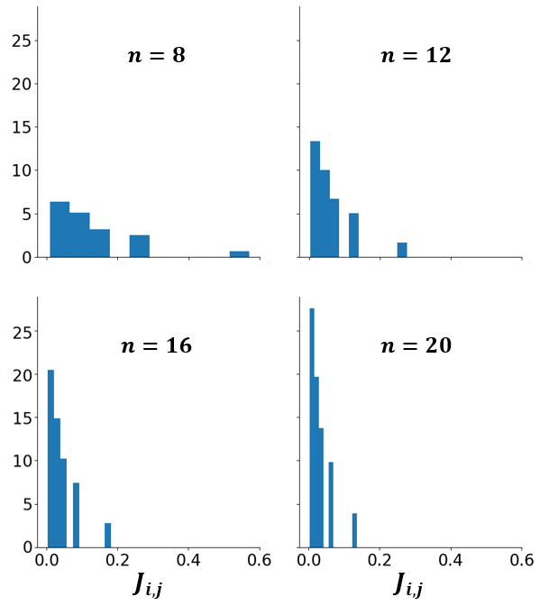
Figure 1: A histogram of all $J_{i,j}$ values for $1000$ portfolio optimization problems for each problem size $n$. This graph is normalized to the probability density.

We use the clique embedding described in Section II for all problem instances. The embedded graphs for the four problems sizes are presented in Fig. 8. These graphs are embedded onto the D-Wave 2000Q processor which is a programmable quantum annealer with a chimera graph structure.

All benchmarks listed in Sec. III are implemented and the $\tilde{p}_{s}$ is found by comparing the quantum annealing solutions to that of a brute force solver which finds the global minimum solution including any degeneracy. The controls studied include varying the chain strength $k$ to observe the effects on the benchmarks as well as post-processing controls which interpret the raw solution returned from the quantum annealer. Other quantum annealing parameters include anneal time which was set to $100\mu s$ and spin reversal which was not implemented for these experiments in order to fully observe the effects of noise and chain strength.

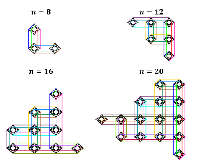
Figure 2: The clique embedding graphs with the Chimera graph structure for problem sizes $n$ where each color represents an embedded chain $V_{T_{i}}$, each diamond grouping of $8$ qubits is a unit cell.

V Results

We first present estimates of the probability of success with respect to chain strength using the discard post-processing method shown in Fig. 3. As expected, $\tilde{p}_{s}$ vanishes for chains with no intra-chain strength while $\tilde{p}_{s}$ increases as chain strength $k$ decreases to about $-1.0$. This is followed by a decrease in $\tilde{p}_{s}$ for smaller $k$, which is an indication that the intra-chain coupling is dominating the spin dynamics. For a fixed value $k$, $\tilde{p}_{s}$ decreases with increasing problem size $n$ while the optimal $k$ varies with $n$. As shown previously in Fig. 1, the distribution of the inter-chain coupling plays an important role in characterizing these problem instances. For the example of $n=8$, the probability of success peaks when the value of $k=-1.0$ for which the maximum $J_{i,j}$ value is $0.57$. However, for all other problem sizes, the optimal intra-chain coupling is observed at $k=-0.5$ for which $J_{i,j}$ is below $0.3$.

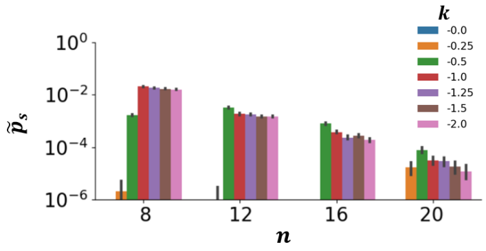
Figure 3: The estimated probability of success $\tilde{p}_{s}$ with respect to intra-chain $k\in[-2,0]$ averaged over $1000$ samples of $1000$ problems for each problem size $n$. All samples with one or more broken chains are discarded (no post-processing) and counted as incorrect.

We differentiate between the type of errors that occur as $k$ decreases by analyzing the probability of broken chains. In Fig. 4, we plot the estimated probability of chain breaks $\tilde{p}_{b}$ with respect to the intra-chain coupling. We observe that samples with $|k|\geq|J_{i,j}|$ have a lower value of $\tilde{p}_{b}$. At $k=0,-0.25,$ and $-0.5$, there is a much higher probability of chains breaking. For weaker $k$, this is shown in Fig. 5 where the average ratio of chain breaks $\tilde{r}_{b}$ reveals that fewer chains break per sample as $k$ increases in strength. At a fixed value of $k=-0.5$, we also observe $\tilde{p}_{b}$ decreases with increasing $n$. As above, we attribute this behavior to the relative differences in magnitude of the inter-chain coupling $J_{i,j}$ and the increased likelihood for chains to break when $k$ and $J_{i,j}$ are close in value.

For all values of $n$, we observe that $\tilde{p}_{b}$ is significantly smaller for $k>-0.5$ than at $k=-0.5$. Notably, there is a small, but consistent, rise in $\tilde{p}_{b}$ at $k=-2$ relative to $k=-1.5$. In addition, $\tilde{p}_{s}$ is reduced in this setting. This combination of behaviors indicates that the errors underlying the reduction in $\tilde{p}_{s}$ are not from chain breaks but due to sampled solutions from excited states. Consequently, we identity a “sweet spot” for the intra-chain coupling that balance the probability of success with probability of chain breaks. The values of $\tilde{p}_{b}$ and $\tilde{r}_{b}$ are also higher at $k=-0.5$ than for weaker $k$. More generally, we expect reductions in $\tilde{p}_{s}$ when $|k|$ is too low in comparison to $|J_{i,j}|$ due to higher $\tilde{p}_{b}$ and also reduction in $\tilde{p}_{s}$ when $|k|$ is too high due to solution drawn from the excited states. These results provide a clear link between the intra-chain coupling parameter $k$ and the error rates impacting $\tilde{p}_{s}$.

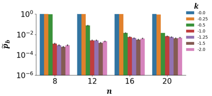
Figure 4: The average probability that a sample has at least one broken chain $\tilde{p}_{b}$ comparing intra-chain strengths $k=[0\rightarrow-2]$ for $1000$ samples of $1000$ problems for each problem size $n$.

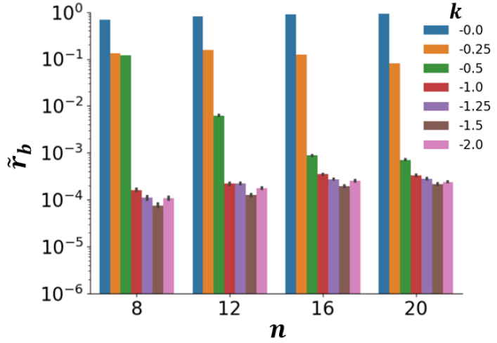
Figure 5: The average ratio of broken chains in a sample $\tilde{r}_{b}$ comparing intra-chain strengths $k=[0\rightarrow-2]$ for $1000$ samples of $1000$ problems for each problem size $n$.

We further investigate the different types of chains break based on where those breaks occur to identify other factors that play a role in error rates. Figure  6 shows the probability for each spin site in a chain to be faulty when at least on chain in the observed sample was broken. As expected, the probability of a chain breaking increases with chain length, in which the latter correlates directly with the problem size $n$. Notably, breaks that occur with the highest probability are always at the endpoint of the embedded chain.

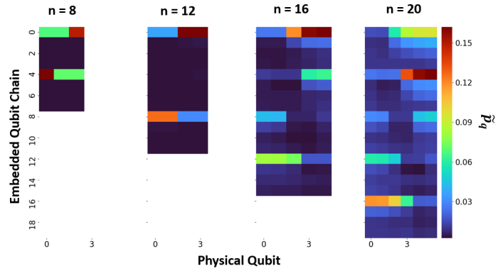
Figure 6: A heatmap showing the average probability for each physical spin in a chain to break for a sample over $1000$ problems each with all broken samples where $k=-0.5$. The comparison is between a set of problems from problem sizes $n$.

There are additional patterns in the observed chains break that reveal a stronger connection to the embedding. As shown in Fig. 6, there is a higher probability of chain breaks at indices $\{0,4,8,12,16\}$. The relative variance in the estimated probabilities range $12\%$ to $25\%$, which is sufficient to identify patterns in the chain breaks that correlated with embedding. Comparing Fig. 6 with the embeddings shown in Fig. 8 reveals broken chains follow a distinct pattern with clique embedding. As shown in Fig. 7, chains with higher values of $\tilde{p}_{q}$, that is, at indices 0, 4, 8, 12, 16, represent chains that utilize the top-most physical qubits across all unit cells.

In addition, the two physical spin sites that break with lowest probability in each of those chains are always coupled within a unit cell as opposed to across unit cells. However, placement on the hardware does not appear to play a strong role in these results. As shown in Fig. 8, our testing recovered similar behaviors from all four problem sizes while using different location for the embeddings within the hardware lattice. These results indicate that $\tilde{p}_{q}$ is linked to the hardware embedding and the physical sites in the unit cell but not the specific unit cells that are employed.

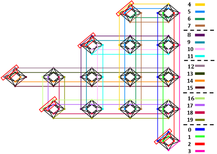
Figure 7: The clique embedding graphs for problem size $n=20$ where the intra-unit cell coupling for embedded chains $0,4,8,12,16$ are boxed and correspond to the spins which have the lowest probability of being faulty for those chains.

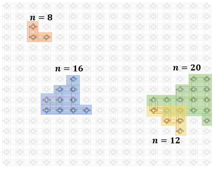
Figure 8: The clique embedding graphs used for all 1000 problems on the D-Wave 2000Q hardware with Chimera graph structure for problem sizes $n$.

We use the detailed information about the frequency and location of chain breaks to tailor methods for post-processing broken chains and assign value to the logical spin. Post-processing strategies that assign a logical value based on the broken chain are more efficient than discarding the sample. We first consider majority vote as a well-known method for post-processing decisions of broken chains. In principle, majority vote works well when the number of errors is small relative to the length of the chain. However, if the intra-chain coupling $k$ is chosen as too weak, then a majority of sites may be broken, and majority vote performs poorly on average.

As shown in Fig. 6, we observe that chains which break with high probability have a majority of their sites broken. Post-processing samples from our benchmarks with majority vote yields the probability of success shown in Fig. 9. Relative to no post-processing, we find that majority vote only increases the probability of success significantly when the probability for chain breaks is greater than 0.1 as is typical for $k>-0.25$.

By contrast, majority vote decreases the probability of success below random selection for $n=8,12$ when $k=-0.25$ due to the bias that emerges from chains with many broken sites. For $k\geq-0.5$, majority vote does not improve the probability of success relative to discarding broken samples. From these observations, we conclude that majority vote does not improve $\tilde{p}_{s}$ when sufficiently high $|k|$ is present. Indeed, an improvement in probability of success by majority vote can serve as an indicator that the intra-chain coupling is insufficient.

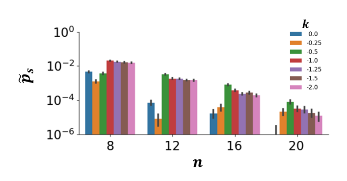
Figure 9: The average probability of success over $1000$ problems each with $1000$ samples where $k$ is varied. The comparison is between a set of problems from problem sizes $8$ to $20$. The post-processing method used is majority vote.

We next apply a post-processing strategy that uses the identified patterns in frequency and location of chain breaks to the benchmark results. Our approach places less weight on sites which are characterized by a higher probability to be faulty within a broken chain. Using the heatmap data shown in Fig. 6 for the clique embedding, we assign values for the embedded logical spins by weighting each physical spin value $q_{l}$ by the probability $\tilde{p}_{q}$. The resulting decisions are given by

$$W_{i}(x_{i})=(1-\prod_{l=0}^{l_{c}}{(\sigma_{l}\tilde{p}^{l}_{q}+\sigma^{\prime}_{l})})\prod_{l=0}^{l_{c}}{(\sigma^{\prime}_{l}\tilde{p}^{l}_{q}+\sigma_{l})}$$ (20)

where $W_{i}(x_{i})$ is the score of the value $x_{i}\in\{-1,1\}$ for logical spin $i$, $\sigma_{l}=(1+x_{i}q_{l})/2=1$ indicates when the value $q_{l}$ of the $l^{th}$ physical spin agrees with the logical choice $x_{i}$ (and zero otherwise), and $\sigma^{\prime}_{l}=(1-x_{i}q_{l})/2=1$ indicates when $q_{l}$ corresponds to the opposing logical choice (and zero otherwise).

The results from this weighted voting strategy are shown in Fig. 10. We find improvements in $\tilde{p}_{s}$ for those cases where there is a high $p_{b}$. This result is far better than a random selection for samples with high $\tilde{p}_{b}$ which demonstrates that there is still some part of the logical problem which survives when $k$ is too weak.

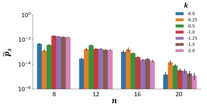
Figure 10: The $\tilde{p}_{s}$ over $1000$ problems each with $1000$ samples where $k=[0\rightarrow-2]$. The comparison is between a set of problems from problem size $n$. The post-processing method used is our custom weighted choice technique incorporating the probabilities of faulty chains.

VI Conclusion

We have benchmarked the behavior of chain breaks for a suite of embedded Hamiltonians across different sizes and parameter settings. By sweeping over a range of intra-chain strengths, we determined the optimal $k$ with varying problem size $n$. We found that the optimal $k$ is strongly linked to the ratio of $J_{i,j}$ to $k$. When the coupling $|k|$ is at or below the $|J_{i,j}|$ range in magnitude $|k|\leq|J_{i,j}|$, the probability for chain breaks increases significantly with a corresponding decrease in the probability to find the correct solution. By contrast, when $|k|$ is too high in comparison to $|J_{i,j}|$, then the probability of chain breaks increases only slightly while the probability of success is found to decrease significantly due to excitations. Thus, these benchmarks identify a ‘sweet spot’ for the intra-chain coupling characterized in terms of the metrics for chains breaks and solution success.

Our results also characterize the frequency and locations with which chain breaks occur in an experimental quantum annealer. Notably, a pattern emerges in the location with the highest probability of chain breaks for our benchmark suite using the clique embedding. By analyzing the probability for each physical spin in an embedded chain to be faulty, we visualized those locations with the highest probability for faults. We found that there are certain chains that break most frequently as indicated by $\tilde{p}_{q}$ strongly correlated with the embedding locations. Chains typically break near the chain edges with the spins coupled within a unit cell statistically least likely to be faulty. We have applied this information about chain breaks to a tailored post-processing method that demonstrates significant improvements in the probability of finding the correct solution.

In conclusion, we have shown how benchmarks for chain breaking reveal sweet spots for optimizing probability of success as well as improved techniques for post-processing strategies. While our results have focused on densely coupled instances of portfolio selection using the clique embedding, we expect similar strategies may be applied across other embedded Hamiltonians. These strategies introduce additional options in the design of computational heuristics based on quantum annealing that can be tuned based on hardware characterization.

References

- [1] Edward Farhi, Jeffrey Goldstone, Sam Gutmann, and Michael Sipser. Quantum computation by adiabatic evolution. arXiv preprint quant-ph/0001106, 2000.
- [2] Tameem Albash and Daniel A Lidar. Adiabatic quantum computation. Reviews of Modern Physics, 90(1):015002, 2018.
- [3] Erica K. Grant and Travis S. Humble. Adiabatic quantum computing and quantum annealing, 07 2020.
- [4] Nicholas Chancellor. Modernizing quantum annealing using local searches. New Journal of Physics, 19(2):023024, 2017.
- [5] Anurag Mishra, Tameem Albash, and Daniel A Lidar. Finite temperature quantum annealing solving exponentially small gap problem with non-monotonic success probability. Nature communications, 9(1):1–8, 2018.
- [6] Jeffrey Marshall, Davide Venturelli, Itay Hen, and Eleanor G Rieffel. Power of pausing: Advancing understanding of thermalization in experimental quantum annealers. Physical Review Applied, 11(4):044083, 2019.
- [7] Mark W Johnson, Mohammad HS Amin, Suzanne Gildert, Trevor Lanting, Firas Hamze, Neil Dickson, Richard Harris, Andrew J Berkley, Jan Johansson, Paul Bunyk, et al. Quantum annealing with manufactured spins. Nature, 473(7346):194–198, 2011.
- [8] John M Martinis, S Nam, J Aumentado, KM Lang, and C Urbina. Decoherence of a superconducting qubit due to bias noise. Physical Review B, 67(9):094510, 2003.
- [9] Shunji Matsuura, Hidetoshi Nishimori, Walter Vinci, Tameem Albash, and Daniel A Lidar. Quantum-annealing correction at finite temperature: Ferromagnetic p-spin models. Physical Review A, 95(2):022308, 2017.
- [10] Sergey Novikov, Robert Hinkey, Steven Disseler, James I Basham, Tameem Albash, Andrew Risinger, David Ferguson, Daniel A Lidar, and Kenneth M Zick. Exploring more-coherent quantum annealing. In 2018 IEEE International Conference on Rebooting Computing (ICRC), pages 1–7. IEEE, 2018.
- [11] Catherine C McGeoch and Cong Wang. Experimental evaluation of an adiabiatic quantum system for combinatorial optimization. In Proceedings of the ACM International Conference on Computing Frontiers, pages 1–11, 2013.
- [12] Helmut G Katzgraber, Firas Hamze, and Ruben S Andrist. Glassy chimeras could be blind to quantum speedup: Designing better benchmarks for quantum annealing machines. Physical Review X, 4(2):021008, 2014.
- [13] James King, Sheir Yarkoni, Mayssam M Nevisi, Jeremy P Hilton, and Catherine C McGeoch. Benchmarking a quantum annealing processor with the time-to-target metric. arXiv preprint arXiv:1508.05087, 2015.
- [14] Bettina Heim, Troels F Rønnow, Sergei V Isakov, and Matthias Troyer. Quantum versus classical annealing of ising spin glasses. Science, 348(6231):215–217, 2015.
- [15] Hartmut Neven, Geordie Rose, and William G Macready. Image recognition with an adiabatic quantum computer i. mapping to quadratic unconstrained binary optimization. arXiv preprint arXiv:0804.4457, 2008.
- [16] Andrew D King and Catherine C McGeoch. Algorithm engineering for a quantum annealing platform. arXiv preprint arXiv:1410.2628, 2014.
- [17] Hayato Ushijima-Mwesigwa, Christian FA Negre, and Susan M Mniszewski. Graph partitioning using quantum annealing on the d-wave system. In Proceedings of the Second International Workshop on Post Moores Era Supercomputing, pages 22–29, 2017.
- [18] Raouf Dridi and Hedayat Alghassi. Prime factorization using quantum annealing and computational algebraic geometry. Scientific reports, 7:43048, 2017.
- [19] Davide Venturelli and Alexei Kondratyev. Reverse quantum annealing approach to portfolio optimization problems. Quantum Machine Intelligence, 1(1-2):17–30, 2019.
- [20] Damian S Steiger, Troels F Rønnow, and Matthias Troyer. Heavy tails in the distribution of time to solution for classical and quantum annealing. Physical review letters, 115(23):230501, 2015.
- [21] Adam Pearson, Anurag Mishra, Itay Hen, and Daniel Lidar. Analog errors in quantum annealing: Doom and hope, 2019.
- [22] Vicky Choi. Minor-embedding in adiabatic quantum computation: Ii. minor-universal graph design. Quantum Information Processing, 10(3):343–353, 2011.
- [23] Christine Klymko, Blair D Sullivan, and Travis S Humble. Adiabatic quantum programming: minor embedding with hard faults. Quantum information processing, 13(3):709–729, 2014.
- [24] Tomas Boothby, Andrew D King, and Aidan Roy. Fast clique minor generation in chimera qubit connectivity graphs. Quantum Information Processing, 15(1):495–508, 2016.
- [25] Timothy D Goodrich, Blair D Sullivan, and Travis S Humble. Optimizing adiabatic quantum program compilation using a graph-theoretic framework. Quantum Information Processing, 17(5):118, 2018.
- [26] Tomas Vyskocil and Hristo Djidjev. Embedding equality constraints of optimization problems into a quantum annealer. Algorithms, 12(4):77, 2019.
- [27] Kristen L Pudenz, Tameem Albash, and Daniel A Lidar. Quantum annealing correction for random ising problems. Physical Review A, 91(4):042302, 2015.
- [28] Walter Vinci, Tameem Albash, Gerardo Paz-Silva, Itay Hen, and Daniel A. Lidar. Quantum annealing correction with minor embedding. Phys. Rev. A, 92:042310, Oct 2015.
- [29] Anurag Mishra, Tameem Albash, and Daniel A Lidar. Performance of two different quantum annealing correction codes. Quantum Information Processing, 15(2):609–636, 2016.
- [30] Jeffrey Marshall, Andrea Di Gioacchino, and Eleanor G. Rieffel. Perils of embedding for sampling problems. Phys. Rev. Research, 2:023020, Apr 2020.
- [31] Erica Grant, Travis Humble, and Benjamin Stump. Benchmarking quantum annealing controls with portfolio optimization, 2020.
- [32] Andrew Lucas. Ising formulations of many np problems. Frontiers in Physics, 2:5, 2014.
- [33] Tameem Albash and Daniel A. Lidar. Decoherence in adiabatic quantum computation. Physical Review A, 91(6), Jun 2015.
- [34] Andrew M. Childs, Edward Farhi, and John Preskill. Robustness of adiabatic quantum computation. Phys. Rev. A, 65:012322, Dec 2001.
- [35] Mohammad HS Amin, Dmitri V Averin, and James A Nesteroff. Decoherence in adiabatic quantum computation. Physical Review A, 79(2):022107, 2009.
- [36] Kevin C. Young, Robin Blume-Kohout, and Daniel A. Lidar. Adiabatic quantum optimization with the wrong hamiltonian. Physical Review A, 88(6), Dec 2013.
- [37] Davide Venturelli, Salvatore Mandra, Sergey Knysh, Bryan O’Gorman, Rupak Biswas, and Vadim Smelyanskiy. Quantum optimization of fully connected spin glasses. Physical Review X, 5(3):031040, 2015.
- [38] Jacek Dziarmaga. Dynamics of a quantum phase transition: Exact solution of the quantum ising model. Physical Review Letters, 95(24), Dec 2005.
- [39] Ryan Hamerly, Takahiro Inagaki, Peter L McMahon, Davide Venturelli, Alireza Marandi, Tatsuhiro Onodera, Edwin Ng, Carsten Langrock, Kensuke Inaba, Toshimori Honjo, et al. Scaling advantages of all-to-all connectivity in physical annealers: the coherent ising machine vs. d-wave 2000q. 2018.
- [40] Zhengbing Bian, Fabian Chudak, Robert Brian Israel, Brad Lackey, William G Macready, and Aidan Roy. Mapping constrained optimization problems to quantum annealing with application to fault diagnosis. Frontiers in ICT, 3:14, 2016.
- [41] Jack Raymond, Ndiamé Ndiaye, Gautam Rayaprolu, and Andrew King. Improving performance of logical qubits by parameter tuning and topology compensation. arXiv preprint arXiv:2006.04913, 2020.
- [42] Inc. D-Wave Systems. Ocean tools library. https://docs.ocean.dwavesys.com/en/stable/.