Measurement of the anomalous precession frequency of the muon in the Fermilab Muon $g-2$ experiment

Abstract

The Muon $g-2$ Experiment at Fermi National Accelerator Laboratory (FNAL) has measured the muon anomalous precession frequency $\omega_{a}^{m}$ to an uncertainty of 434 parts per billion (ppb), statistical, and 56 ppb, systematic, with data collected in four storage ring configurations during its first physics run in 2018. When combined with a precision measurement of the magnetic field of the experiment’s muon storage ring, the precession frequency measurement determines a muon magnetic anomaly of $a_{\mu}({\rm FNAL})=116\,592\,040\,(54)\times 10^{-11}$ (0.46 ppm). This article describes the multiple techniques employed in the reconstruction, analysis and fitting of the data to measure the precession frequency. It also presents the averaging of the results from the eleven separate determinations of $\omega_{a}^{m}$, and the systematic uncertainties on the result.

I Introduction

Reference [1] reports a new measurement of the muon magnetic anomaly $a_{\mu}=(g_{\mu}-2)/2$ made by our Muon $g-2$ Collaboration based on its Run-1 data at Fermi National Accelerator Laboratory (FNAL). That initial physics run occurred over a period of 15 weeks in Spring 2018. We find

$$a_{\mu}({\rm FNAL})=116\,592\,040\,(54)\times 10^{-11}.$$

where the total uncertainty includes the dominant statistical uncertainty combined with combinations from the precession rate systematic, magnetic systematic, and beam-dynamics systematic uncertainties. This combined uncertainty corresponds to a $0.46$ parts per million (ppm) measurement.

Three companion papers to that letter describe in detail the key inputs to this result. Reference [2] presents the detailed analysis of the precision measurement of the magnetic field within our storage ring. Reference [3] details the small corrections to our anomalous moment measurement from effects associated with the dynamics of the stored muon beam. This paper presents the data reconstruction, analysis, and systematic uncertainty evaluation for the determination of the average muon spin precession frequency within the precision magnetic field of our storage ring. The letter brings the results from these three papers together, combining the corrected muon precession frequency with the precision field measurement to obtain the $a_{\mu}$ result given above.

I.1 Status of $g-2$ of the muon

The measurement of the muon magnetic anomaly performed by the E821 experiment at the Brookhaven National Laboratory (BNL) [4] of $a_{\mu}=116\,592\,092(63)$ has shown an excess with respect to the Standard Model (SM) prediction by over 3.5 standard deviations. Since the publication of the final E821 result, the evaluation of the SM prediction has undergone significant scrutiny. The quantum electrodynamics (QED) contributions to $g-2$, calculated to order $(\alpha/\pi)^{5}$ [5, 6], agree well with precise measurement of $g-2$ for the electron [7]. Recent discrepancies in the measurement of the fine structure constant [8, 9] do not significantly affect the muon $g-2$ prediction. Electroweak corrections include the complete two-loop evaluation, hadronic effects, and the leading log 3-loop contributions [10, 11, 12]. The dominant theoretical uncertainties arise in the QCD hadronic vacuum polarization (HVP) and hadronic light-by-light (HLxL) corrections, which the Muon $g-2$ Theory Initiative [13] has recently reviewed thoroughly. The review, covering dispersive, lattice and modeling methods, arrived at a consensus [14] for the hadronic contributions and their uncertainties, and predicts $a_{\mu}^{SM}=116\,591\,810(43)\times 10^{-11}$ [5, 6, 15, 16, 17, 18, 19, 20, 21, 22, 23, 24, 25, 26, 27, 28, 29, 30, 31, 32]. Comparison with the E821 result yields a difference of $(279\pm 76)\times 10^{-11}$, which remains over the 3.5 standard deviation level. In order to confirm, or refute, that discrepancy, Experiment E989 [33] was constructed at Fermi National Laboratory.

I.2 Principles of the experiment

The Fermilab E989 (Muon $g-2$) experiment follows a sequence of polarized muon beam storage experiments pioneered at CERN and BNL. In particular, it uses an experimental approach based on the muon anomalous precession within a storage ring with a highly uniform and precisely known magnetic field. This approach was pioneered in the CERN experiment [34] and refined with muon, rather than with pion, injection by the E821 experiment at BNL [4].

The technique is based on the convergence of three fundamental effects: the relative precession rates of the muon spin and momentum within a uniform magnetic field, parity violation in muon decay, and the Lorentz boost of the muon decay products between the muon rest frame and the lab frame. When a muon orbits horizontally within the uniform vertical magnetic field of a perfect storage ring, its momentum vector precesses at the cyclotron frequency $\vec{\omega}_{c}=-q\vec{B}/m\gamma$. For a relativistic muon polarized in the horizontal plane, the Larmor precession, combined with Thomas precession, yields a total spin precession frequency of

$$\vec{\omega}_{s}=-g_{\mu}\frac{q\vec{B}}{2m}-(1-\gamma)\frac{q\vec{B}}{m\gamma}.$$

The relative precession frequency of the spin with respect to the momentum, denoted hereafter as the anomalous precession frequency $\omega_{a}$, is therefore

$$\vec{\omega}_{a}=\vec{\omega}_{s}-\vec{\omega}_{c}=-\left(\frac{g_{\mu}-2}{2}\right)\frac{q\vec{B}}{m}=-a_{\mu}\frac{q\vec{B}}{m}.$$ (1)

A measurement of the anomalous precession frequency, coupled with precise knowledge of the storage ring magnetic field, therefore provides a direct probe of the anomalous magnetic moment.

Parity violation within the weak decay of the muon provides the means for such a direct measurement of the anomalous precession frequency: the highest energy positrons from muon decay are emitted, within its rest frame, in a direction strongly correlated with the muon spin direction. When coupled with the Lorentz boost, this spin-energy correlation results in a modulation of the positron energy spectrum in the laboratory frame: the stiffest spectrum occurs when the spin and muon momentum directions are aligned, and the softest occurs when they are anti-aligned. This modulation occurs at the rate of the anomalous precession frequency.

As a result of the energy modulation, the number of positrons above a given energy threshold $E_{\rm th}$ from muon decay within this ideal stored beam varies with time as

$$N(t)=N_{0}e^{-t/\gamma\tau_{\mu}}\left(1+A(E_{\rm th})\cos(\omega_{a}t+\phi_{0})\right).$$ (2)

The parameter $N_{0}$ represents the initial beam intensity, $\gamma\tau_{\mu}$ the lifetime of the boosted muon, and $\phi_{0}$ the average initial angle of the muon spins relative to the beam direction. The asymmetry parameter $A(E_{\rm th})$, which governs the amplitude of the rate oscillation about the average exponential for muon decay, depends on the threshold energy: the energy-spin correlation weakens as the positron energy decreases. In fact, since the total decay rate must fall as a pure exponential, the asymmetry, evaluated for the lowest energy positrons, changes sign. The choice of energy threshold then requires balancing the increased muon statistics with the dilution of the average asymmetry, and the optimal choice varies with the method used to extract the anomalous precession frequency (see Sec. VI). Details of the statistical power of the $\omega_{a}$ determination are described in [4] where it is shown that, for the optimal method, the variance of the measured precession frequency $\omega_{a}$ scales as

$$\sigma^{2}\propto\frac{1}{N\langle A^{2}\rangle_{E_{\rm th}}}\,.$$ (3)

While a vertical magnetic field provides the horizontal confinement necessary to store a muon beam, storage of the beam for any significant period requires additional vertical focusing. A pulsed electrocstatic quadrupole (ESQ) system, comprising four discrete sections symmetrically spaced about the muon storage ring and covering 43% of its circumference, provides this focusing. Allowing for the presence of such an electric field $\vec{E}$, as well as for muon beam motion that is not strictly perpendicular to the magnetic field, the anomalous precession frequency of Eq. 1 becomes  [3]

$$\vec{\omega}_{a} = -\frac{q}{m}\left[a_{\mu}\vec{B}-a_{\mu}\left(\frac{\gamma}{\gamma+1}\right)(\vec{\beta}\cdot\vec{B})\vec{\beta}\right.$$ (4)

$$\left.-\left(a_{\mu}-\frac{1}{\gamma^{2}-1}\right)\frac{\vec{\beta}\times\vec{E}}{c}\right].$$

The $\vec{\beta}\cdot\vec{B}$ term accounts for a possible component of the muon velocity parallel to the magnetic field. The last term, which corresponds to the additional magnetic field component that the muon experiences in its rest frame from $\vec{E}$, vanishes for a muon with momentum $p_{0}=3.094$ GeV/c, or $\gamma\sim 29.3$. This experiment has been designed to accept and store a beam of muons with a narrow momentum spread (0.15%) about $p_{0}$. The corrections to $a_{\mu}$ arising from both vertical beam motion and the residual electric field correction are discussed in detail in Ref. [3]. Due to these and to other effects detailed in [1], the measured precession frequency needs to be corrected in order to obtain the quantity $\omega_{a}$ required to evaluate $a_{\mu}$. This paper describes the procedure followed to obtain the observed precession frequency $\omega_{a}^{m}$. After the corrections to bring this observed frequency to the ideal $\omega_{a}$ above, combination with the precision field measurements detailed in Reference [2] allow determination of $a_{\mu}$.

Muons stored at this momentum possess a boosted lifetime of $\gamma\tau_{\mu}\approx\,$$64.4\text{\,}\mathrm{\SIUnitSymbolMicro s}$. This lifetime limits the practical storage time of the beam: almost all of the muons have decayed away after $700\text{\,}\mathrm{\SIUnitSymbolMicro s}$. We therefore need many muon beam “fills”, cycles of muon beam injection and storage, which occur at a rate of 16 fills every 1.4 s for E989. In each fill, a muon bunch of time width 120 ns, to be compared with a cyclotron period $T_{c}=$149.2\text{\,}\mathrm{n}\mathrm{s}$$, is injected within the 7.112 m radius ring, with its 1.45 T field.

The muons within the storage ring undergo betatron oscillations – stable oscillations about the equilibrium orbit – with characteristics that depend on the strength of the ESQ electric field. The system is weak-focusing and properly characterized by the field index $n$ for a continuous ESQ given by

$$n=\frac{R_{0}}{vB_{0}}\frac{\partial E_{y}}{\partial y},$$ (5)

where $R_{0}$ is the equilibrium orbit radius, $v$ is the muon velocity, $B_{0}$ is the magnetic field, and $E_{y}$ is the effective vertical quadrupole field component. The horizontal ($x$) and vertical ($y$) tunes – the number of betatron oscillations per cyclotron revolution – are related to the field index by $\nu_{x}\approx\sqrt{1-n}$ and $\nu_{y}\approx\sqrt{n}$, respectively. These tunes introduce two key oscillation frequencies into the experiment,

$$f_{x} \approx f_{c}\sqrt{1-n}$$ (6)

$$f_{y} \approx f_{c}\sqrt{n}.$$ (7)

with $f_{c}=\omega_{c}/2\pi$. The radial and vertical betatron motion of the muons within the beam is strongly coherent when the beam is first injected into the storage ring. The lattice chromaticity, due to the $\sim 0.15\%$ momentum spread of the stored muon beam, and the ESQ non-linearities, related to higher order multipoles, cause this motion to decohere.

The finite acceptance of the detector system couples with the beam motion resulting from coherent betatron oscillations (CBO) to introduce additional time modulation into the rate of detected positrons and into the shape of the positron energy spectrum. As Sec. VI and Ref. [2] discuss in detail, these CBO effects introduce a time variation into the effective asymmetry $A(E_{\rm th})$ and phase $\phi_{0}$ terms in Eq. 1. Radial motion of the beam (within the horizontal plane) introduces particularly strong oscillations at multiples of the frequency $f_{CBO}=f_{C}-f_{x}$. Accurate modeling of the time dependence of our data requires incorporation of both the horizontal and vertical effects. The betatron oscillations do not, though, couple strongly to the anomalous precession frequency $\omega_{a}^{m}$ as long as they are stable while the muons are stored.

Table 8, in the Appendix, summarizes the nominal frequencies that characterize the $g-2$ storage ring for the two values of the field index employed during Run-1.

The remainder of this article proceeds as follows. After a summary of the instrumentation relevant for the precession frequency analysis in Section II, Section III presents the analysis strategies behind the determination of the precession frequencies, followed by the data reconstruction strategies employed to enable those strategies in Section IV. Section V outlines the two major corrections applied to the data: the gain corrections input to the reconstruction and the pileup correction needed before fitting. Section VI then presents the data model, the fit, the fit results and the stability of the fit results. After a discussion of the systematic uncertainties affecting the precession measurement in Section VII, the article concludes with a discussion of the averaging procedure to combine the results from the different analysis efforts in Section VIII, followed by the summary of results in Section IX.

II Instrumentation overview

The primary system for measurement of the positron energy and time distribution consists of a suite of 24 small electromagnetic calorimeters distributed around the interior of the storage ring and positioned behind a scallop in the vacuum chamber to minimize the material traversed by the daughter positrons, as shown in Fig. 1. The positrons from muon decay, have momenta too small to be stored in the ring and drift inwards in the magnetic field towards the calorimeters. At any given time, a single calorimeter will detect positrons emitted from muons over only a small range of spin precession phases. The highest energy positrons can travel a significant fraction of an orbit before encountering a calorimeter. Softer positrons travel smaller distances, so have been produced later in a muon precession cycle. As a result, the phase of the muon when it decayed varies over the energy range of accepted daughter positrons. The phase difference over this range does not significantly dilute the precession signal.

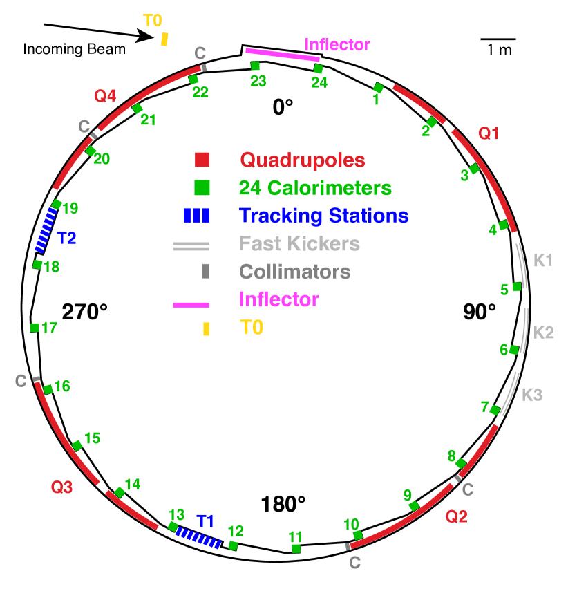
Figure 1: Schematic of the Muon $g-2$ storage ring and instrumentation showing the elements directly involved in the muon precession analysis. Key elements include the suite of 24 electromagnetic calorimeters (green or medium grey), the straw tracker system (dark blue or near back), the ESQs (red or dark grey), a fast kicker system (light blue or light grey), and the beam entrance (T0) detectors (yellow or very light grey).

Each calorimeter station, described in detail elsewhere [35, 36, 37], consists of a 9 column by 6 row array of PbF₂ crystals instrumented with silicon photomultiplier (SiPM) photodetectors. Digitization of the output from each of the $24\times 54$ channels occurs continuously over an entire fill at a rate of approximately 800 Megasamples per second (MSPS). This scheme eliminates dead time and potential rate-dependence. A beam-arrival signal from the Fermilab accelerator complex triggers the digitization process for a fill. The master digitization clock for the experiment is completely independent of the accelerator clocks that determine the beam-arrival timing. Blinding of the precise digitization rate at the hardware level avoids the potential for unconscious bias in the data analysis. During data analysis, an additional level of blinding occurs in software, as described in Sec. VI.3.

The blinded clock for digitization derives from a master 40 MHz precision clock, in turn driven by a GPS-stablized 10 MHz rubidium clock source. To achieve the hardware-level blinding, two Fermilab staff (independent of the collaboration) detune the 40 MHz clock to a frequency in the range 39,997 kHz to 39,999 kHz. Correction for the blinding offset occurred as the last stage of the analysis, after completion of all systematic bias evaluations and cross checks, and following the decision to unblind and publish. We mix a second blinded clock with the master clock to monitor the clock system stability without revealing the blinding offset. The monitoring of the resulting blind frequency difference utilizes a second GPS-stabilized reference clock that is completely independent of the master clock and its GPS stabilitization.

The set of complete waveforms obtained from a fill then pass to the frontend processors of the data acquisition (DAQ) system [38] for data reduction, which proceeds as follows. Each calorimeter has a dedicated frontend processor and GPU that perform the data reduction necessary to keep the stored data volume manageable. The DAQ system prepares two data streams for offline analysis. The first “event-based” data stream corresponds to identification of particle activity within the detector. Whenever a waveform sample for any crystal in a calorimeter exceeds a $\sim 50$ MeV threshold, the DAQ system extracts a time window of approximately $40\text{\,}\mathrm{\SIUnitSymbolMicro s}$, depending on the pulse width, surrounding that sample from all crystals in that calorimeter for offline analysis. The second data stream provides a continuous sampling of the waveforms for each fill that allows an “integrated energy” approach (Sec. VI) to the precession frequency determination. To achieve a manageable data output rate, the DAQ system combines the raw crystal waveform samples into contiguous 75 ns windows over a range of $-$$6\text{\,}\mathrm{\SIUnitSymbolMicro s}$ to $+$$231\text{\,}\mathrm{\SIUnitSymbolMicro s}$ relative to the muon beam arrival time for the Run-1 data presented here. The system also allows summing of a configurable number of consecutive fills, but that was not utilized for this dataset.

For the measurement of $\omega_{a}^{m}$, time stability relative to the start of the fill drives the design of the detector as well as the data reconstruction algorithms. Suppose, for example, the gain of the SiPM photodetectors drift in a fashion correlated with time since muon injection (referred to as “time into the fill”). Without correction, the true positron energy distribution above a fixed threshold in an analysis would shift. Because of the energy-precession phase correlation discussed above, such a shift would effectively introduce a time dependence into the phase $\phi_{0}$ in the precession term in the decay rate (Eq. 2). With $\phi_{0}\rightarrow\phi(t)$, the extracted precession phase $\omega_{a}$ would be directly biased . A laser-based system [39] provides monitoring and assessment of such gain variations in each of the 1296 crystals. The system sweeps a set of laser pulses over the time into the fill on a subset of data and directly measures the beam-correlated gain variations. This system also provides a common pre-beam pulse, for each fill, that allows time synchronization of all of the digitizer channels and it is used to monitor time stability across the fill.

Reconstruction effects that are sensitive to particle flux, and thus can vary early to late, can also introduce an effective $\phi(t)$ and a possible bias to $\omega_{a}^{m}$. These effects, such as random overlap of different positron showers in a calorimeter (pileup), will be noted in later sections of the paper.

Several other subsystems indicated in Fig. 1 play a role in the analysis of the spin precession data. The T0 counter, located at the beam entrance to the storage ring, provides a measurement of the beam arrival time, which is used as the reference start time for the spin precession measurements. The signal from this counter is digitized within the same system as the calorimeters and also receives the common laser time synchronization pulse. A fast kicker system [33] places the injected beam onto a trajectory that allows stable storage. The amplitude of the momentum kick affects the amplitude of the CBO that must be modeled in the data. Finally, two stations of straw trackers [33] allow the measurement of effects arising from the dynamics of the stored beam that affect analysis of the data.

II.1 Run-1 data subsets

Over the course of the Run-1 dataset, the pulsed high voltage systems (fast kicker and electrostatic ESQs) operated at several different set points as we commissioned them and tuned for optimal running conditions. These systems play significant roles in determining the beam dynamics, such as the amplitude and frequency of the CBO, which in turn can modulate the positron rate. We therefore determine $\omega_{a}^{m}$ during each operating condition individually. Table 1 summarizes the key characteristics of these four data subsets.

Table 1: Summary of the Run-1 data subsets. The positron statistics correspond to those with energy greater than 1.7 GeV after a time of $30\text{\,}\mathrm{\SIUnitSymbolMicro s}$ into a fill, according to the selection criteria described in section III.1.

Run-1	Tune	Kicker	Fills	Positrons
Subset	(n)	(kV)	($10^{4}$)	($10^{9})$
1a	0.108	130	151	0.92
1b	0.120	137	196	1.28
1c	0.120	130	333	1.98
1d	0.107	125	733	4.00

During this physics run, two of the 32 high voltage resistors for the ESQs became damaged. While the ESQs still operated, the resulting change in resistance altered the RC time constant for some ESQ plates and increased the time required to reach operating voltages. As a result, some of the voltages varied at the beginning of the time window used for the determination of $\omega_{a}^{m}$. This variation introduced a time dependence into the CBO-related frequencies, which could be measured directly and incorporated into the $\omega_{a}^{m}$ analyses (see Sec. VI). The variation also introduced a time dependence to the beam width. Because the average muon precession phase varies across the transverse beam storage volume (due to positron acceptance effects), this change of width introduced a time-dependent drift to the average precession phase $\phi(t)$. Such a phase drift shifts the observed precession frequency and must be corrected. Reference [3] discusses the determination of the beam storage related corrections to $\omega_{a}^{m}$ for these four subsets in detail.

III Analysis techniques

By pursuing multiple independent analyses of the muon spin precession data, we obtain powerful cross checks on the value of the precession frequency $\omega_{a}^{m}$ determined from the data. For the Run-1 results described here, six analysis efforts have been developed, each utilizing a unique mix of reconstruction, analysis and independent data-driven corrections to determine $\omega_{a}^{m}$. These approaches have varying sensitivities to potential systematic effects, as well as varying statistical sensitivities. This section summarizes the four general analysis approaches that have been used to determine $\omega_{a}^{m}$ from the Run-1 data, as well as the common selection criteria. The six efforts draw from these four techniques to arrive at a total of eleven determinations of $\omega_{a}^{m}$ for each data subset. The following sections provide the details of data reconstruction, data correction and fitting.

Reference [40] provides a detailed mathematical analysis of the statistical sensitivity for each of the approaches described here.

III.1 Data selection

The data selection criteria applied in all analyses include fill-level discriminants that ensure that all critical subsystems, such as the electrostatic quadrupoles (ESQs), the fast kickers and all the calorimeter channels were operating in a standard, stable condition. The criteria identify and eliminate, for example, time intervals surrounding sparking in the ESQ system. Additional criteria ensured stable, uniform conditions for delivery of the beam to the storage ring, as well as stable magnetic field conditions.

All analysis methods select reconstructed positron candidates (Sec. IV.1) or integrated energy samples (Sec. IV.2) that are at least $30\text{\,}\mathrm{\SIUnitSymbolMicro s}$ into the fill after beam injection. Prior to $30\text{\,}\mathrm{\SIUnitSymbolMicro s}$, programatic variation of the ESQ plate voltages moves the beam edges into collimators to reduce the population of muons at the boundaries of phase space accepted by the storage ring [3]. This procedure helps to minimize beam loss during the period over which we observe the muon spin precession. By $30\text{\,}\mathrm{\SIUnitSymbolMicro s}$, the ESQ plates stabilize at their nominal value. This start time choice also reduces other effects, like event pileup (Sec. V.2), related to high detector rates at injection time that could potentially bias $\omega_{a}^{m}$, yet strikes a reasonable balance with statistical losses.

For the Run-1d subset, we shift the analysis starting time to $50\text{\,}\mathrm{\SIUnitSymbolMicro s}$ into the muon fill because of effects related to the damaged ESQ high voltage resistors. Ref. [3] discusses these effects and their corrections in detail.

In all analyses, the precise start time of the fit corresponds to a node in the anomalous precession cycle, which minimizes the sensitivity to time-dependent effects like a gain change correlated with time into the fill. The end time of the fit is at $T\simeq\,$$650\text{\,}\mathrm{\SIUnitSymbolMicro s}$, corresponding to approximately 10 muon lifetimes at $p_{0}=3.094$ GeV/c.

III.2 Event-based methods

Within the event-based approach, an analysis selects candidate decay positron events reconstructed with energies above an optimal threshold, and bins them in time relative to beam injection. The different methods correspond to different positron weighting schemes. These methods reflect the physical process described in Sec. I.2, in which the positron rate asymmetry grows with increasing energy threshold because of the increasing correlation between decay positron direction and muon spin. With unit weighting per positron ($w(E)=1$), this method maps directly onto the rate prediction of Eq. 2, though with additional effects from positron acceptance and beam dynamics. Alternatively, weighting each positron by the effective decay asymmetry at its energy ($w=A(E)$) provides the optimal statistical sensitivity [40]. Four of the analysis efforts for Run-1 use both the threshold method, with unit weighting, and the asymmetry-weighted method. Each team extracts the asymmetry function $A(E)$ directly from the data by binning the data in positron energy $E$ and fitting the time distribution in each bin (see Sec. VI for a discussion of the fitting method).

The inverse of the $\omega_{a}^{m}$ variance scales as $N\bar{A}^{2}$ for the threshold method, where $N$ represents the total positron statistics above threshold and $\bar{A}$ the average asymmetry, and as $NA_{\rm rms}^{2}$ for the asymmetry-weighted method, where $A_{\rm rms}$ is the root mean square asymmetry above threshold. Figure 2 illustrates the behavior of these two statistical figures of merit (FOM) from a simple Monte Carlo simulation that includes basic detector acceptance effects but assumes perfect knowledge of the absolute energy scale. For the threshold method, the lower energy positrons dilute the asymmetry to an extent that overwhelms the statistical gains, causing the overall sensitivity to drop off. For the asymmetry-weighted method, the asymmetry weighting itself minimizes the dilution, and, in principle, it allows using positrons of all energies, including those of negative asymmetry.

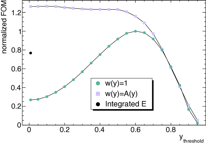
Figure 2: The statistical figures of merit $N\bar{A}^{2}$ calculated using a simple Monte Carlo simulation for the threshold method ($w(y)=1$) and $NA_{\rm rms}^{2}$ for the asymmetry-weighted method ($w(y)=A(y)$) as a function of threshold energy. The simulation included basic detector acceptance. The normalized energy $y=E_{e^{+}}/E_{\rm max}$, where $E_{\rm max}\approx 3.1$ GeV is the maximum allowed positron energy in the laboratory frame from muon decay. The isolated black point indicates the corresponding figure of merit for the integrated energy method in case of no energy threshold (Sec. III.3).

In practice, acceptance, detector effects and uncertainties in the absolute energy scale all affect the optimal choice of energy threshold. For the threshold method, a sweep over a range of threshold energies determines the optimal threshold from the data itself. At each trial threshold energy, a fit to the time-binned data with the ideal functional form of Eq. 2 provides the $\omega_{a}^{m}$ precision estimate. Figure 3 shows a representative sweep. The optimal threshold occurs near 1.7 GeV for the threshold method. For the asymmetry-weighted method, a 1.0 GeV threshold choice balances detector noise mitigation with the marginal statistical gain from a lower threshold.

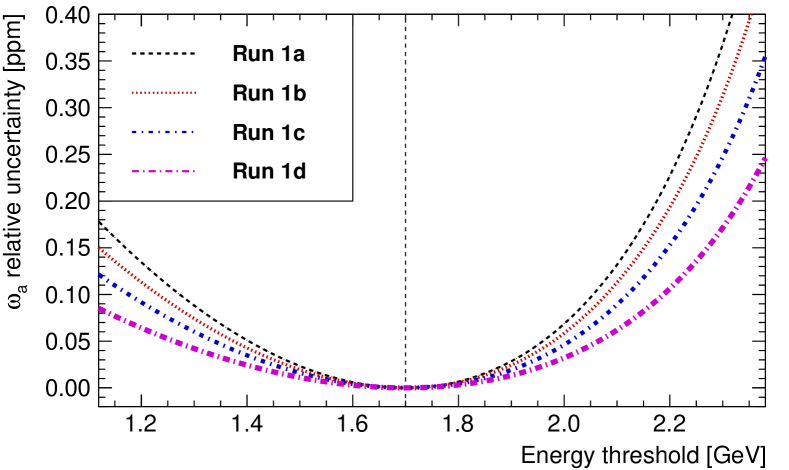
Figure 3: Relative uncertainty on $\omega_{a}^{m}$ versus energy threshold for the four Run-1 datasets determined from a simple five-parameter fit (cf. Eq. 2) to data with varying threshold. The different curvature is due to the different statistics among the datasets.

III.3 Integrated energy method

The integrated energy method extracts the anomalous precession frequency from the calorimeter data with a very different strategy. Rather than using disjoint time windows with discrete positron events, this method examines a continuous total energy sum in the calorimeters from a combination of many muon fills. An energy versus time histogram is then formed from this data. This method uses different raw data and analysis procedures, thus inheriting different systematic sensitivities and providing complementary statistics. In particular, contributions from pulse pileup events and the initially bunched muon beam, both key issues in controlling systematic effects, require very different handling. As such, the integrated energy method, although statistically less powerful, remains valuable in demonstrating the robustness of the extraction of the anomalous frequency.

III.4 Ratio method

The ratio method, described in detail in Ref. [41], provides a way of processing the data to remove the exponential decay and reduce any slowly or smoothly varying effects in the data, such as muon losses. This method can be combined with any of the event-based or integrated energy approaches. For the Run-1 results presented here, we have applied this technique to a threshold method analysis. Elimination of these slowly varying effects shifts the relative importance of different systematic sensitivities compared to the event-based analyses.

To eliminate the slow variations, this method randomly divides the positron candidates into four subsets. When time binning the data, the times for one subset receive a shift forward by $T_{a}/2$, where $T_{a}$ is the anomalous precession period , those in a second subset receive a shift backwards by $T_{a}/2$, while those in the other two remain unchanged. In terms of the number of events $n(t)$ collected in the bin at time $t$, the rebinning process yields the four binned functions

$$u_{+}(t) =\frac{1}{4}n(t+T_{a}/2),$$ (8)

$$u_{-}(t) =\frac{1}{4}n(t-T_{a}/2),$$ (9)

$$v_{1}(t) =\frac{1}{4}n(t),$$ (10)

$$v_{2}(t) =\frac{1}{4}n(t),$$ (11)

Forming the sum and difference ratio

$$r(t)=\frac{[u_{+}(t)-v_{1}(t)]+[u_{-}(t)-v_{2}(t)]}{[u_{+}(t)+v_{1}(t)]+[u_{-}(t)+v_{2}(t)]},$$ (12)

suppresses the exponential decay term and other slowly varying effects. Re-expressing the yields $n(t)$ in terms of the rate function in Eq. 2 and expanding in $(T_{A}/\gamma\tau_{\mu})$ the functional form of the ratio becomes

$$r(t)=A\cos{(\omega_{a}^{m}t+\phi)}-\frac{1}{16}\left(\frac{T_{a}}{\gamma\tau_{\mu}}\right)^{2}+\\ {\cal O}\left((T_{a}/(4\gamma\tau_{\mu}))^{4}\right),$$ (13)

which illustrates the suppression of the lifetime. Figure 4 presents the ratio function obtained from the Run-1d data subset.

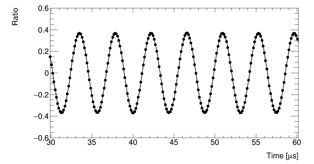
Figure 4: The ratio $r(t)$ (see text) obtained from the Run-1d data subset. The ratio preserves the amplitude and the frequency of the $g-2$ oscillation, while eliminating the exponential behavior and reducing other slow and smooth terms.

Reweighting the four rebinned subsets according to

$$u_{+}(t):u_{-}(t):v_{1}(t):v_{2}(t)=\\ e^{T_{a}/2\gamma\tau_{\mu}}:e^{-T_{a}/2\gamma\tau_{\mu}}:1:1$$ (14)

eliminates the last two terms in Eq. 13 and a simple sinusoidal description of the ratio time series becomes exact in the absence of beam-related effects. Those effects, such as betatron oscillations and muon loss, do not cancel exactly in the ratio, therefore this analysis approach utilizes the full functional form of $r(t)$ described in Sec. VI.

All bins in the $u$ and $v$ functions for Run-1 contain sufficient statistics to allow standard Gaussian error estimation and propagation. With the lifetime correction factors incorporated into the definition of the $u$ functions, the expression for the statistical uncertainty on the $r(t)$ binned ratios becomes

$$\sigma_{r}^{2}(t)=\frac{1-r^{2}(t)}{u_{+}(t)+u_{-}(t)+v_{1}(t)+v_{2}(t)}.$$ (15)

This provides a statistical uncertainty that is comparable to the event-based methods.

III.5 Finite beam length

At injection time, the 120 ns long beam does not spread evenly along the storage ring. As a result, the initial positron intensity at individual calorimeter stations oscillates at the cyclotron frequency ($T_{c}=$149.2\text{\,}\mathrm{n}\mathrm{s}$$). The beam, however, debunches because higher momentum muons orbit at larger radii, and therefore with longer periods, than lower momentum muons. After $5\text{\,}\mathrm{\SIUnitSymbolMicro s}$, the leading edge of the beam first laps the trailing edge. By the analysis start time of $30\text{\,}\mathrm{\SIUnitSymbolMicro s}$ (approximately two hundred orbits), the muon beam populates the ring almost uniformly. Figure 5 shows the positron intensity variation in one calorimeter from the residual beam bunching.

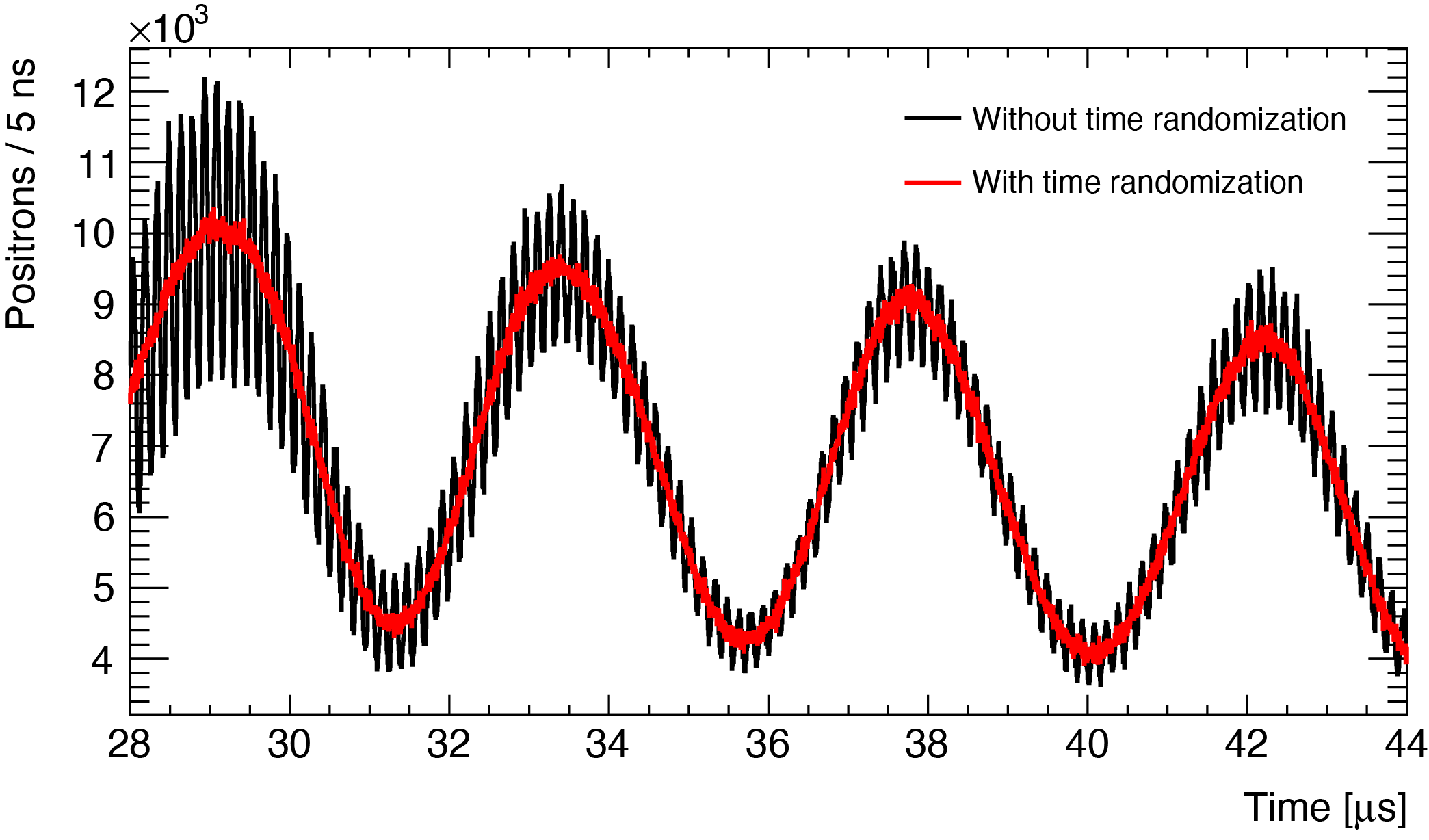
Figure 5: The positron intensity variation in one calorimeter as a function of time. Unrandomized data (black) clearly show a variation at the $149.2\text{\,}\mathrm{n}\mathrm{s}$ cyclotron periodicity on top of the slower ($4.365\text{\,}\mathrm{\SIUnitSymbolMicro s}$) $\omega_{a}^{m}$ variation from the residual beam bunching. Time-randomization of the data (red or grey) suppresses this variation, and binning in the cyclotron period suppresses further to a negligible level. Data are from a subset of Run-1.

Combining the positron data in widths of the average $T_{c}$ largely filters out this effect, leaving only a small residual sinusoidal trend in $\omega_{a}^{m}$ as a function of calorimeter position. Because of the varying phase of this signal around the ring, summing data from all calorimeters almost completely eliminates the residual effects. As Fig. 5 also shows, randomizing the measured positron arrival times uniformly over the interval $\pm T_{c}/2$ while binning eliminates this effect, even at the calorimeter level. All event-based $\omega_{a}^{m}$ analysis approaches for Run-1 employ this randomization procedure.

IV Data reconstruction

The two raw data paths from the DAQ system, event and integrated energy based approaches as discussed in Section II, require distinct reconstruction algorithms. For the event-based analyses, the data reconstruction stage transforms the raw waveform data in each saved time window into positron candidates with quantities such as positron hit energies and times. We have independently developed two methods for this positron reconstruction: local-fitting and global-fitting. Both fitting approaches utilize pulse templates, empirical descriptions of each individual SiPM’s response to positron showers and laser pulses, to extract times and energies from digitizer waveforms. We construct the template for each channel using the data, and each template includes the well-defined oscillatory behavior for that channel after the main pulse, which results from imperfections in the pole zero subtraction in the SiPM readout electronics. The physics objects resulting from the two methods will necessarily differ somewhat because of diverging decisions made during the respective algorithm and software development processes. These differences between reconstruction procedures aid in characterizing and understanding each approach. Applying multiple reconstructions to the same raw data helps verify correctness of the reconstruction and provides an important check on systematic effects.

For the integrated energy analysis, the reconstruction involves careful combination of the contiguous waveforms over all crystals and all muon fills to obtain a final integrated waveform that preserves a good signal to noise ratio.

IV.1 Local-fitting approach

The local approach fits pulses with an amplitude over a configurable threshold in each crystal independently. References [42, 36] describe the template pulse fitting algorithm utilized in this step in detail. Should two or more pulses occur within the length of the pulse template (250 ns), the algorithm refits them simultaneously, using the results of the initial fits as starting parameters, to remove effects due to the tail of the first pulse overlapping with the second one. This fitting algorithm correctly handles scenarios in which multiple pulses spread over two or more distinct time windows from the DAQ system, as shown in Fig. 6.

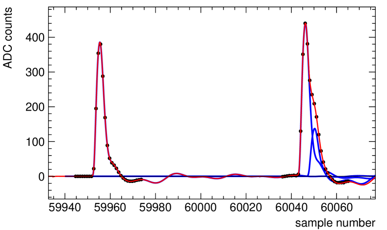
Figure 6: Example of a template fit selected from Run-1 data. The black points are digitizer sample values and the smooth curves are fit results. Each “sample number” corresponds to 1.25 ns. This figure shows a chain fit containing waveforms from two separate time windows and three pulses. The baseline perturbations from the first pulse persist into the second time window, in which two pulses separated by 5 ns were identified.

The individual pulses receive relative energy and timing alignment corrections determined from studies of the minimum-ionizing-particle (MIP) signal from muons passing through the calorimeters [43]. Timing of all calorimeter channels gets aligned to the muon beam arrival time through a synchronization (sync) pulse generated by the laser system. All calorimeter channels and the T0 detector receive this common sync pulse. The difference from the sync pulse time for the calorimeter channels’ sample times compared to the beam arrival time in the T0 detector provides the aligned time into fill for all channels. Sec. V.1 discusses the application of gain corrections on various timescales. The location of the optimal $\omega_{a}^{m}$ threshold in each calorimeter (see Fig. 3) then sets the absolute energy scale.

The final step of reconstruction involves the clustering of pulses from individual channels into a candidate positron with an estimate of the total energy of the incident positron. The clustering combines all pulses in a calorimeter station within a tunable artificial dead time window into one candidate. We have used windows of both 3 ns and 5 ns for the Run-1 analyses. During clustering, the impact position of the positron is also inferred using a center-of-gravity method with logarithmic weights [44, 45]. For more details about the local reconstruction approach, please refer to Sec.4 of Ref. [46]. While not used for the Run-1 analysis, spatial clustering can be added to the time-based one.

IV.2 Global-fitting approach

In the global-fitting approach, the algorithm simultaneously fits clusters of pulse waveforms from multiple crystals in a given time window from the DAQ. This approach inherently imposes spatial separation between positrons that hit a calorimeter close in time, reducing the size of the pileup correction discussed in Sec. V.2.2. In particular, each positron with an energy over a threshold of 60 analog-to-digital counts (ADC), corresponding to approximately 50 MeV, above noise is identified with a $3\times 3$ cluster of crystals. After applying a time correction to each crystal similar to that described in Sec. IV.1, the clusters identified in the time window are fit by minimizing a $\chi^{2}$ described in Section VI.4. Because the SiPM pulse shape for a crystal does not depend on the pulse magnitude [36], we can model each trace by a crystal-dependent template that scales with energy and translates with time. The pulse magnitude for each crystal pulse floats independently in the fit. The algorithm constrains the templates for each crystal to peak at a shared time. Clusters that share one or more crystals must be separated by at least 1.25 ns; otherwise, they will be merged into one larger cluster. When a pulse template extends across multiple time windows, the algorithm refits all identified clusters within these windows simultaneously. Relative energy corrections determined using the MIP energy peak from muons adjust the pulse amplitude for each crystal in the cluster. An $\omega_{a}^{m}$ energy threshold scan determines the absolute energy, similarly to the local-fitting approach (Fig. 3). A refined version of the center-of-gravity method with logarithmic energy weights provides an estimate of the position of each cluster. For more details about this reconstruction approach, refer to Ch. 4 in Ref. [45].

IV.3 Integrated energy waveform

As discussed in Sec. II, 1296 contiguous, time-rebinned, crystal-by-crystal waveforms comprise the integrated energy dataset. These waveforms span a time period of $-$$6\text{\,}\mathrm{\SIUnitSymbolMicro s}$ $\,<t<+$$231\text{\,}\mathrm{\SIUnitSymbolMicro s}$ relative to the beam arrival time with $75$ ns wide bins. The reduced time range and increased time binning were chosen to limit the rate and volume of the integrated energy data. Ideally, a simple sum of the waveforms over the 54 crystals from a calorimeter would yield the integrated energy waveform for that calorimeter. As Fig. 7 illustrates, while positron pulses appear clearly in single-fill waveforms, the O($100\,$ns) pedestal recovery structure overwhelms the positron precession signal in the waveform over all fills in a dataset. We have therefore developed a threshold integration method to separate the integrated time distribution from the pedestal variation.

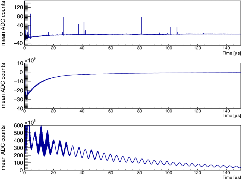
Figure 7: Representative single-fill rebinned waveforms for a high rate crystal in Calorimeter 12 (top), the corresponding waveform sum over all crystals and all fills in Run-1c for Calorimeter 12 (middle), and the above threshold integrated energy waveform (bottom). The vertical axis of time-decimated ADC counts is the mean value of the 60 raw ADC samples of each time-decimated bin. The beam injection and pedestal recovery signals appear clearly for both the single-fill and summed time distributions. While individual positron pulses appear clearly in the single-fill distributions, the pedestal structure overwhelms their contribution in the summed distribution.

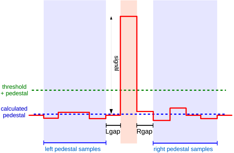
Figure 8: Diagram illustrating the pedestal calculation algorithm and the application of the threshold for the threshold integrated energy waveforms. The mean of the below-threshold samples in the left / right pedestal window provides the pedestal estimate. $L_{\rm{gap}}$ / $R_{\rm{gap}}$ are adjustable gaps between the time bin and the left / right pedestal windows.

Fig. 8 depicts the threshold integration method. For each fill-level crystal waveform from a calorimeter, a rolling pedestal algorithm provides a pedestal estimate at each time bin. After gain correction (see Sec. V.1), any pedestal-subtracted energy that exceeds a pre-defined threshold setting is added to the threshold integrated energy waveform $E(t)$ for that calorimeter.

In the Run-1 analysis, the mean value of the below-threshold ADC samples in equal-sized time windows to the left and right of each time bin provides the pedestal estimate. To avoid biases from pulse undershoot and ringing in the estimate, the algorithm introduces a gap between the pedestal windows and the time bin. The threshold setting, pedestal window size, and gap size are all adjustable parameters common to all crystals. The nominal settings in processing Run-1 data correspond to a threshold setting of $\sim$300 MeV, left and right pedestal windows of 300 ns, and left and right gap sizes of 75 ns.

While the event based methods use time randomization to ameliorate the residual effects of the finite beam length (see Sec. III.5), correction of the integrated energy waveform requires a different approach. Combining the above waveforms pairwise into $T_{b}=150$ ns wide bins, which is close to the cylcotron period $T_{c}=$149.2\text{\,}\mathrm{n}\mathrm{s}$$, would suppress these effects. However, an aliased modulation at a frequency $f_{\rm alias}=1/T_{c}-1/T_{b}$ would persist. We instead employ a smoothing algorithm to combine the 75 ns binned waveform $\{E_{i}^{75}\}$ into the 150 ns binned waveform $\{E_{i}^{150}\}$ via

$$E^{150}_{i}=\frac{1}{4}E^{75}_{2i-1}+\frac{1}{2}E^{75}_{2i}+\frac{1}{4}E^{75}_{2i+1}.$$ (16)

where $i$ refers to the bin number of the 150 ns wide binned data. This approach eliminates both the fundamental and the aliased modulations. While the procedure introduces bin-by-bin correlations, these can be accommodated straightforwardly in subsequent fitting procedures.

The associated uncertainties for the above-threshold, integrated energy, histogram bins were computed using Poisson statistics. Given a bin energy $E=\sum_{j}E_{j}$, obtained by summing recorded positron energies $E_{j}$, the associated bin uncertainty is $\sigma=(\sum_{j}E^{2}_{j})^{1/2}$. Small corrections arise from effects of positron pileup and the division of a positron’s energy between two adjacent time bins. Such effects are order 10^-2 on the normalized $\chi^{2}$.

V Data corrections

A number of time-dependent effects require application of corrections to the reconstructed data to avoid bias in $\omega_{a}^{m}$. These effects include gain variations on a number of timescales, pileup effects in the calorimeters, and the loss of beam muons through mechanisms other than decay.

V.1 Detector gain fluctuation and time synchronization

The energy scale of each calorimeter channel can vary with external factors such as temperature and hit rate. These effects occur over different timescales: hours or days for temperature-related effects, and microseconds or tens of microseconds for effects related to muon rate. A laser calibration system [39] provides the ability to correct for these effects. The system operates in different modes to provide correction functions at different time scales: long-term correction for daily effects, in-fill gain correction for the tens of microseconds scale, short term gain correction for hits which are tens of nanoseconds apart.

The above-mentioned effects affect the physics output in different ways. In particular, any variation of the calorimeter response between the beginning and the end of a fill, if uncorrected, results in a early-to-late energy threshold variation and thus in a potential shift of $\omega_{a}^{m}$ as mentioned in Sec. II.

The E989 systematic uncertainty goal related to detector gain variation is 20 ppb, which requires control of systematic gain changes over the $700\text{\,}\mathrm{\SIUnitSymbolMicro s}$ long muon fills better than 0.5 per mille (see Fig. 16.5 in [33]). The long-term corrections, which do not couple as directly to the determination of $\omega_{a}^{m}$, do not require as strict a control.

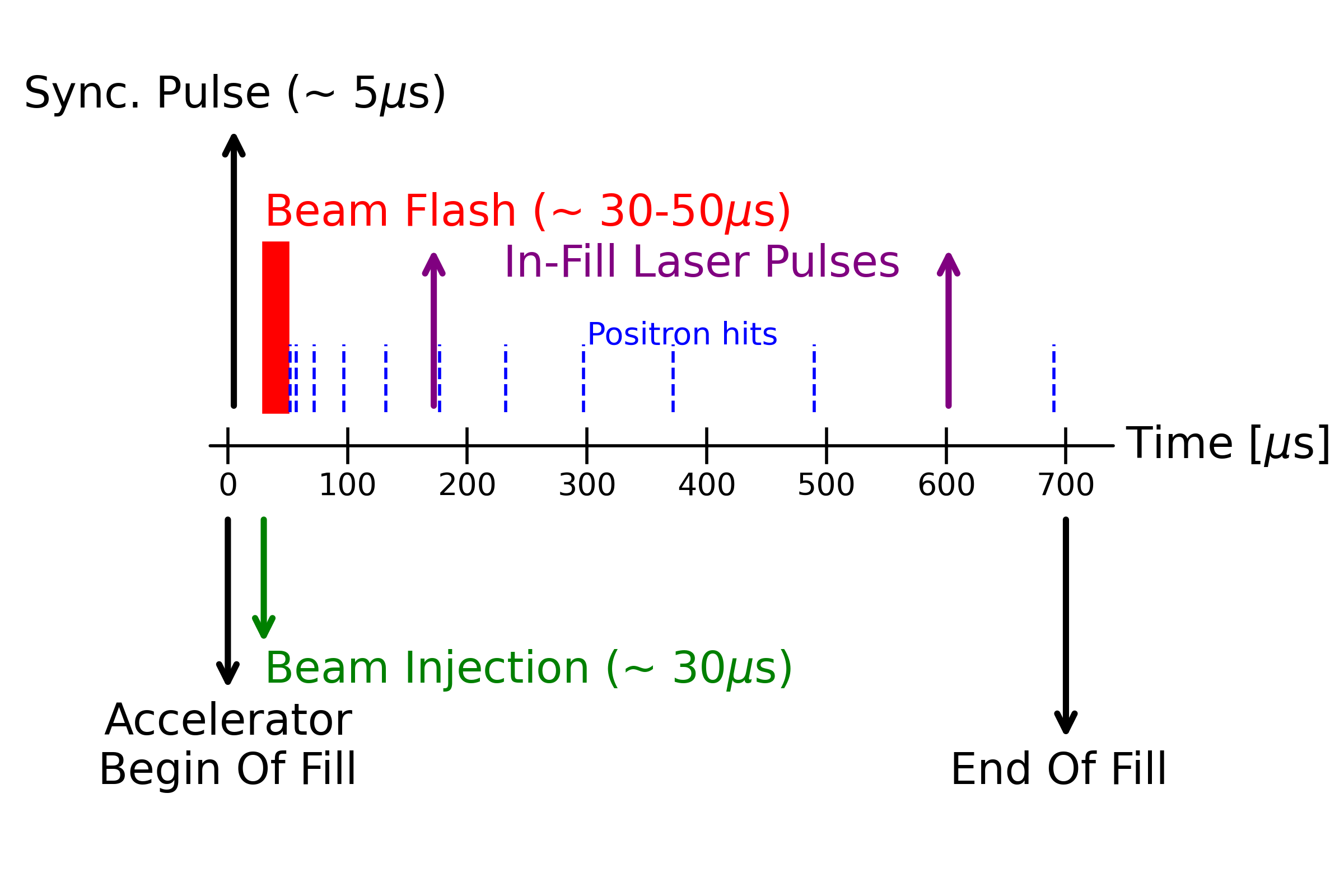
Figure 9: Timing of the sync pulse and representative in-fill pulses provided by the laser system.

Reference [39] provides details of the laser system. Briefly, a programmable Laser Control Board triggers a pattern of laser pulses which illuminate, during standard data taking, the calorimeter crystals through quartz fibers coupled to the crystal face. The amount of emitted light approximately corresponds to an energy release of 1 GeV. Figure 9 shows a schematic of this pattern, which includes a reference signal issued before injection that provides precise time synchronization, and a set of pulses during a fraction of the muon fills that accurately measure the detector response as a function of rate. An additional set of pulses between fills (not shown) provide the long term calibration. The fills with laser pulses are not to be used for the analysis, as the laser itself modifies the detector response. Therefore only a fraction of approximately 10% of the muon fills include the laser pulses.

Figure 10 shows a representative gain curve for a single crystal, as measured by the laser calibration system, during the first $200\text{\,}\mathrm{\SIUnitSymbolMicro s}$ after muon injection. The initial gain sag, clearly visible at the time of injection, results from SiPM charge depletion that occurs when the initial flash of particles, accompanying the storable muon beam at injection, strikes the calorimeters.

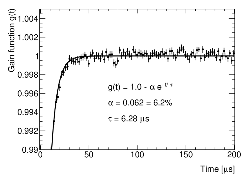
Figure 10: The gain function describes the gain drop in the photodetection system for a representative calorimeter channel due to the flash of muons and beam positrons at injection. It is expanded to show the behavior of the gain after $t=30\,\mu s$, the starting time of the $\omega_{a}^{m}$ fit (see section III.1).

A model for the gain function based on an exponential decay returning asymptotically to unity, with average amplitude of approximately 6% and time constant of order $6\text{\,}\mathrm{\SIUnitSymbolMicro s}$, adequately describes the calorimeter response to laser data. Thus $30\text{\,}\mathrm{\SIUnitSymbolMicro s}$ after injection, the start time of the $\omega_{a}^{m}$ fit, the gain correction is at the per mille level and it rapidly decreases to zero. While small, this correction is not negligible and its effect on $\omega_{a}^{m}$ is discussed in Sec. VII.1.

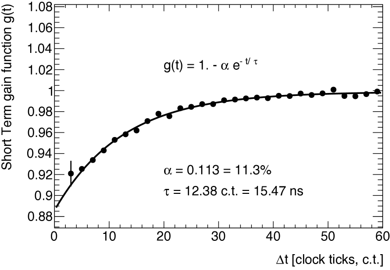
Figure 11: Gain correction function for consecutive hits in the same crystal as a function of their time separation expressed in clock ticks. The clock sampling frequency is 800 MHz and 1 clock tick corresponds to 1.25 ns.

When two positrons hit the same crystal within a few tens of nanoseconds, the finite recovery time of the SiPM and amplifier can reduce the gain experienced by the second particle. We map this short term gain correction as a function of energy and time by redirecting the laser light so that two lasers can pulse a set of crystals with programmable delay and intensity. Figure 11 shows the gain drop for a typical channel. The amplitude varies linearly with the energy of the first particle with an average slope of 5%/GeV, while the exponential recovery time has an average value of $15\text{\,}\mathrm{n}\mathrm{s}$.

While the short time correction can be readily applied to the event-based analysis, in which single positron clusters are selected, the integrated energy method requires a different approach. A second in-fill gain correction is determined which combines the gain drop effects due both to the initial muon flash and to the hit of consecutive positrons, providing an average combined correction.

V.2 Multi-positron pileup

The positron reconstruction approaches described in Sec. IV cannot resolve multiple positrons that strike a calorimeter sufficiently close in time or space. Event-based analyses must account for such pileup by statistically subtracting a constructed pileup spectrum. Without this correction, the unresolved pileup could bias the fitted $\omega_{a}^{m}$ in Sec. VI by as much as $\mathcal{O}(100~{}\text{ppb})$. The integrated energy approach, by design, has no inherent pileup bias, in the limit of zero energy threshold, because it looks only at total energy and does not need to associate energy contributions to individual positrons. This subsection presents three different approaches developed to correct for the pileup contamination present in the spectrum of reconstructed positrons.

V.2.1 Shadow window approach

The shadow window approach described here builds on and refines the original algorithm developed for the BNL E821 experiment [4]. Reference [41] provides further details on the algorithm and attendant modifications of the statistical uncertainties of the positron data.

The algorithm assumes that the probability of observing a pileup positron (doublet) equals that for observing two individual positrons (singlets) that are separated in time by an amount much smaller than the cyclotron period. The shadow window method searches in a fixed time window after a given positron (the trigger) for a second trailing positron (the shadow). A time offset $T_{G}$, also called shadow gap time, from the trigger and a shadow window width $T_{D}$ define the search window.

When the shadow window contains a positron, the trigger (T) and shadow (S) positrons are combined into a shadow doublet with energy and time

$$E_{\text{doublet}}=C\cdot(E_{\rm T}+E_{\rm S}),$$ (17)

$$t_{\text{doublet}}=\frac{t_{\rm T}\cdot E_{\rm T}+(t_{\rm S}-T_{G})\cdot E_{\rm S}}{E_{\rm T}+E_{\rm S}}+\frac{T_{G}}{2}.$$ (18)

The constant $C$ in the energy sum corrects for a response difference of the calorimetry for true pileup compared to the resolved positrons. The Run-1 analyses employing the shadow window approach use the nominal value $C=1$. The energy-weighted time of the two singlets provides the time for the doublet, with a shift of $T_{G}/2$ that accounts for the muon flux variation across that gap time.

Application of this procedure to all time-ordered positron candidates within each fill provides a data driven statistical estimate of the pileup contamination. Pileup distorts the data time distribution by adding the doublets while removing the individual positron contributions. Therefore the difference

$$P(E,t)=D(E,t)-S_{T}(E,t)-S_{S}(E,t),$$ (19)

where $D(E,t)$ is the distribution of doublets, and $S_{T}(E,t)$ and $S_{S}(E,t)$ are the distribution of trigger and shadow singlets respectively, provides the correction to be subtracted from the reconstructed time series. The single positrons used to build up the doublet enter in $S_{T}(E,t)$ and $S_{S}(E,t)$ shifting their time to $t=t_{D}$.

For the Run-1 analyses that employ the shadow window method, the shadow window width $T_{D}$ is tuned depending on the specific analysis artificial dead time parameters, with a value typically close to 5 ns. The shadow gap time $T_{G}$, typically near 10 ns, has been tested for values ranging from 10 ns up to the beam cyclotron period of $\sim 150$ ns.

V.2.2 Empirical approach

The shadow window approach is based on models for how the reconstruction in Sec. IV.1 would treat two positron hits close in time or space. To avoid such modeling challenges, we have developed a more empirical approach where the multiple pulses are superimposed at the waveform level [45]. The use of the reconstruction directly on the combined waveforms eliminates the need for modeling behavior of the global reconstruction (Sec. IV.2).

This algorithm first identifies pairs of reconstructed clusters that spatially overlap and fall within $149.2\pm 5.0$ ns of each other, corresponding to a cyclotron period. For each pair, the raw time windows are corrected for gain effects, such as the short term effect (Sec. V.1), and superimposed. The reconstruction algorithm is then run on this combined time window (Sec. IV.2) and in case a single cluster is identified, it populates the energy-time distribution $\rho_{1+2}(E,t)$, while the original clusters populate $\rho_{1}(E,t)$ and $\rho_{2}(E,t)$. The difference

$$\delta\rho_{\text{pileup}}(E,t)=\frac{\rho_{1+2}(E,t)-\rho_{1}(E,t)-\rho_{2}(E,t)}{2}$$ (20)

provides the pileup spectrum correction, with the factor of $1/2$ correcting for combinatorics. Subtracting $\delta\rho_{\text{pileup}}(E,t)$ from the reconstructed spectrum statistically corrects it for pileup.

Because pileup contaminates the sample of single clusters themselves, the pileup spectrum in Eq. 20 requires a correction for higher-order pileup. In particular, each of the two singlets is contaminated by the two-positron pileup rate, so the next order correction can be determined by extending the above procedure to include triplets of reconstructed clusters. The above superposition and reconstruction procedure of different combinations of three raw waveforms produces four energy-time distributions, one for the triple combination and one for each of the three pairings. The combination

$$\delta \rho_{\text{correction}}(E,t)$$

$$= -\left[\rho_{1+2+3}(E,t)-\rho_{1}(E,t)-\rho_{2}(E,t)-\rho_{3}(E,t)\right]/2$$

$$+\left[\rho_{1+2\phantom{+3}}(E,t)-\rho_{1}(E,t)-\rho_{2}(E,t)\right]/2$$

$$+\left[\rho_{2+3\phantom{+1}}(E,t)-\rho_{2}(E,t)-\rho_{3}(E,t)\right]/2$$

$$+\left[\rho_{1+3\phantom{+2}}(E,t)-\rho_{1}(E,t)-\rho_{3}(E,t)\right]$$ (21)

gives the correction to be added to Eq. 20 (for details see [45]). The indices on the energy-time distributions indicate the time order of original cluster candidates when the corresponding waveforms are superimposed. For Run-1, no corrections beyond this order are necessary to sufficiently correct the reconstructed spectra for pileup.

As in the case of the shadow window approach, the determination of $\omega_{a}^{m}$ from the pileup-subtracted time series uses an exact calculation of the bin uncertainties [45].

Overall, this empirical approach provides an excellent description of the pileup events present in the reconstructed data. This method is also robust against modifications to the reconstruction algorithm. In addition, it avoids the need for simulation to characterize, for example, the possible dependencies of $C$ in Eq. 17. Ref. [45] provides further detail about the procedures and characterization for this approach.

V.2.3 Probability density function approach

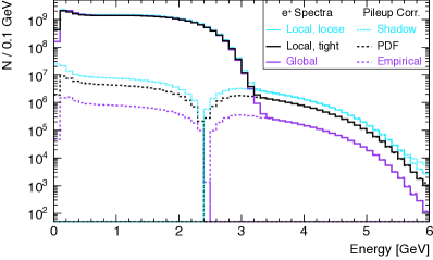
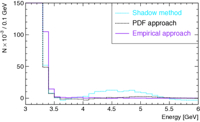
Figure 12: Measured energy spectrum, summed over all calorimeters, along with the total pileup correction. Left: number of positrons per energy interval. The three solid curves correspond to the uncorrected spectra from the different clustering procedures, the global-fitting approach (purple or dark gray), local-fitting with tight clustering cuts (black), and local-fitting with loose clustering cuts (blue or light gray). The dashed lines correspond to the associated pileup correction evaluated with three different methods: empirical approach (purple or dark gray), probability density function approach (black), shadow method approach (blue). The correction curves show the absolute value of the pileup contribution, which has a negative sign (events to be subtracted from energy spectrum) above $E\sim 2.4$ GeV and a positive sign (events to be added to the energy spectrum) below $E\sim 2.4$ GeV. Right: The corrected spectra obtained from the (signed) difference between solid and dashed lines for the three methods. Few residual events remain in the unphysical region above the endpoint of the spectrum which, due to detector resolution, extends up to $E\sim 3.4$ GeV.

Unlike the previous approaches, where the pileup spectrum is created by “combining” two clusters or waveforms, the probability density function approach constructs the pileup spectrum by considering the energy-time distribution of an entire dataset.

Let $\rho(E,t)$ represent the ideal calorimeter hit distribution that would be measured by a detector with perfect resolution in time and space and $\delta\rho_{pu,d}(E,t)$ the double pileup perturbation. The sum $\rho_{pu,d}(E,t)=\rho(E,t)+\delta\rho_{pu,d}(E,t)$ describes the effect of two-particle pileup $\rho_{pu}(E,t)$. A leading-order estimate of $\delta\rho_{pu,d}(E,t)$ yields [46]

$$\begin{array}[]{l}\delta\rho_{pu,d}(E,t)=\\ r(t)\cdot\Delta t\bigg{[}\rho_{d+}(E,t)-2\rho(E,t)\int\rho(E_{2},t)\mathop{}\!\mathrm{d}E_{2}\bigg{]}~{},\end{array}$$ (22)

with the double pulse sum term defined as

$$\rho_{d+}(E,t)\equiv\int\rho(E-E_{2},t)\cdot\rho(E_{2},t)\mathop{}\!\mathrm{d}E_{2}.$$ (23)

The parameters $\Delta t$ and $r(t)$ represent the detector reconstruction dead time and the overall hit rate as a function of time, respectively. The first term in Eq. 22 corresponds to the false counts measured when two positron showers are mistaken for one, and the second term corresponds to the two true positron showers that are lost. The former will in principle be affected by nonlinearities in the treatment of unresolved pulse pairs by the reconstruction. These nonlinearities are not included in the pileup correction approach described here.

Eq. 22 describes the contamination of the measured energy spectrum from double pileup in terms of the uncontaminated spectrum $\rho(E,t)$. By iterative application of the expression starting with the measured hit spectrum, which is itself contaminated by pileup, Eq. 22 can also generate the pileup correction. Because the relative double pileup contamination appears at the order $r(t)\cdot\Delta t$, even with a conservative detector reconstruction dead time and no spatial cluster separation employed in the reconstruction, $r(t)\cdot\Delta t$ distorts the term in brackets by at most 1% to 2%. Thus, use of the pileup contaminated hit spectrum, instead of the ideal one, to generate the expected double pileup contamination distorts the correction by order $r^{2}(t)\Delta t^{2}$, or $10^{-4}$. Repeating this procedure using the spectrum $\rho_{c}(E_{2},t)$ obtained from the first correction estimate yields a final spectrum also correct to order $r^{2}(t)\Delta t^{2}$. These key observations motivate this pileup correction method. One can also determine the expected contamination from triple pileup, which appears at order $r(t)^{2}\Delta t^{2}$.

The treatment of double pileup shown above assumes that all pulse pairs within the detector reconstruction dead time of one another will yield a false count at the summed energy and the loss of a count at each of the two constituent pulse energies. This assumption is not valid when three pulses all fall within the reconstruction dead time. In this case, one expects a loss of three true counts and a gain of one false count. A simple application of the double pileup treatment, however, would count three pulse pairs and thus erroneously remove six true counts and add three false counts. A triple pileup correction must then account both for the reconstruction’s treatment of groups of three unresolved pulses and for the error in the double pileup correction that occurs at the order of triple pileup. Ref. [46] shows that the correction

$$\begin{array}[]{l}\delta\rho_{pu,t}(E,t)=\\ r(t)^{2}\Delta t^{2}\bigg{[}\int\rho(E-E_{d})\cdot\rho_{d+}(E_{d},t)\mathop{}\!\mathrm{d}E_{d}\\ -3\rho_{d+}(E,t)\cdot\int\rho(E_{3},t)\mathop{}\!\mathrm{d}E_{3}\\ +3\rho(E,t)\cdot\left(\int\rho(E_{2},t)\mathop{}\!\mathrm{d}E_{2}\right)^{2}\bigg{]}\end{array}$$ (24)

removes the triple pileup perturbation. The bias in the triple pileup correction from use of the pileup-contaminated spectrum, rather than the true one, is of order $r(t)^{3}\cdot\Delta t^{3}$, or $10^{-6}$.

Ref. [46] provides the details of the implementation of this method. As done for the other two methods, each final bin uncertainty of the corrected spectrum includes the contribution from this procedure.

Figure 12 summarizes, for the three methods, the initial pileup contribution (left) and the residual contamination above the positron end point (right) after pileup subtraction.

V.2.4 Pileup and the threshold integrated energy analysis

Conceptually, a threshold-free integrated energy analysis is free from distortion by pileup of positrons in space and time. The integrated energy correctly receives the energy contribution from all positrons – whether proximate or not.

However, a threshold-based integrated energy analysis can suffer pileup distortions. Therefore, an algorithm was developed for calculating the pedestal and applying the threshold that mitigated such distortions.

To understand the algorithm it is important to note that pileup pulses may occur either on the trigger sample or in the pedestal window. A pileup pulse on the trigger sample will increase the corresponding, pedestal-subtracted, ADC value. A pileup pulse in the pedestal window will decrease the corresponding, pedestal-subtracted, ADC value.

By requiring both the trigger sample to be above the energy threshold and the pedestal samples to be below the energy threshold, the effects of pileup are mitigated. To understand this mitigation it is important to note the four categories of pulse pileup: an above-threshold pulse on the trigger sample, an above-threshold pulse in the pedestal window, a below-threshold pulse on the trigger sample, and a below-threshold pulse in the pedestal window.

1. An above-threshold pileup on the trigger sample is properly handled as the correct energy of the two above-threshold pulses on the trigger sample is recorded

2. An above-threshold pileup in the pedestal window is properly handled as the correct energy of the single above-threshold pulse on the trigger sample is recorded due to rejection of the above-threshold pileup pulse in the pedestal window,

3. A below-threshold pileup on the trigger sample causes an overestimate of the correct energy of the single above-threshold pulse on the trigger sample.

4. A below-threshold pileup on the pedestal window causes an underestimate of the correct energy of the single above-threshold pulse on the trigger sample. However, overall, the energy overestimation from below-threshold, trigger sample pileup and energy underestimation from below-threshold, pedestal window pileup, statistically cancel.

Extensive studies with Monte Carlo simulations show that the residual contribution from higher-order pileup has negligible effect on $\omega_{a}^{m}$.

VI Determination of $\omega_{a}^{m}$

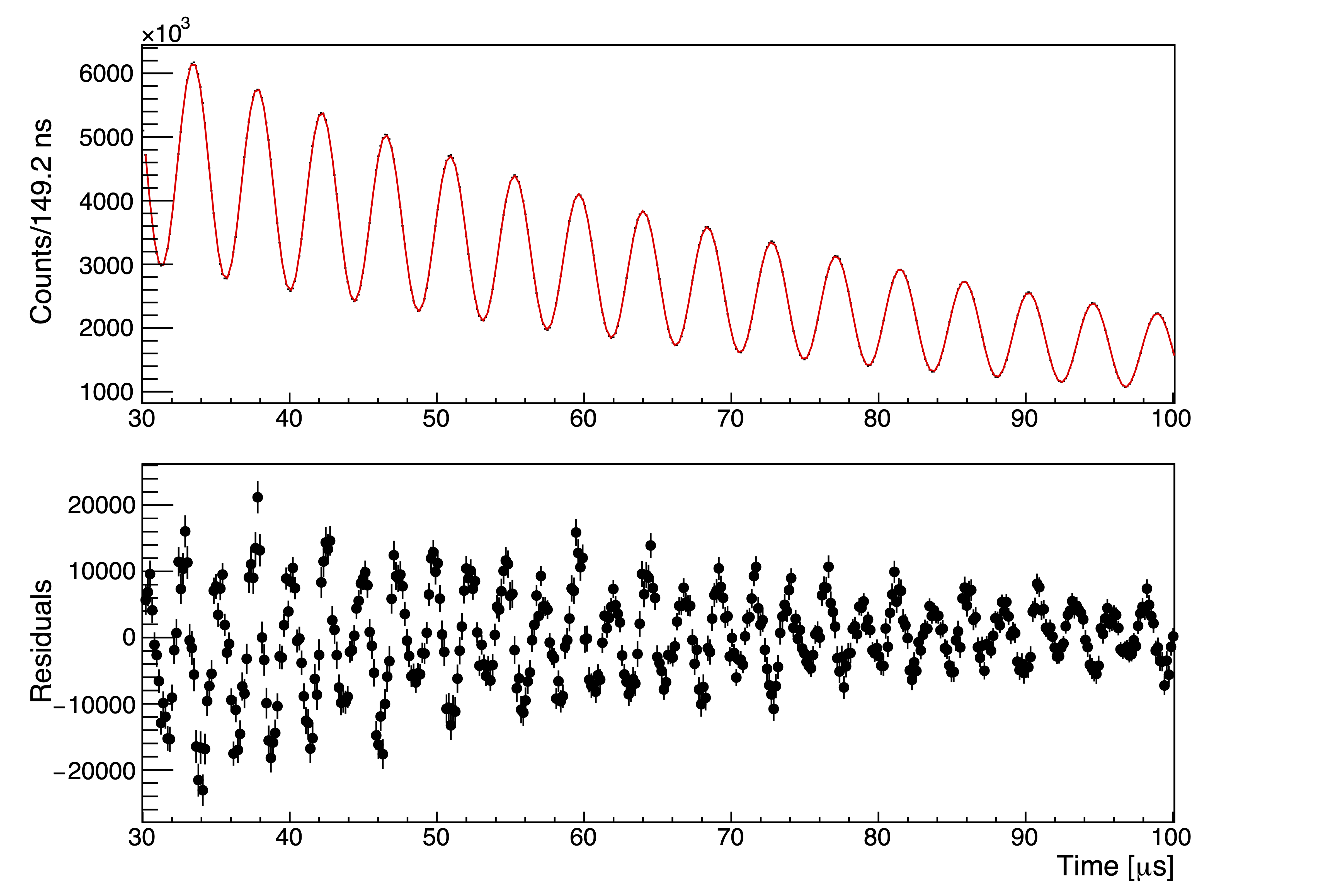
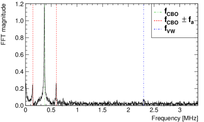
Figure 13: The results of a five-parameter fit based on Eq. 2 to the time series from the unit-weighted event analysis of the Run-1a data. Left: the fit at early times (top) and the fit residuals (bottom), showing beam effects that the simple five-parameter function does not describe. Right: Fourier transform of the fit residuals showing the peaks at the expected beam oscillation frequencies. These distributions emphasize the need to incorporate the effects related to the beam dynamics into the fit model, as discussed in the text.

An unbiased determination of $\omega_{a}^{m}$ requires a physically motivated functional form that describes the positron time series detected by the calorimeters. This section discusses the dynamical effects included in our fitting model, and the fits to determine the anomalous precession frequency.

Figure 13 shows the function and residuals for the first $70\text{\,}\mathrm{\SIUnitSymbolMicro s}$ of a five-parameter fit (Eq. 2) to the time series from the unit-weighted event analysis of the Run-1a data. As discussed earlier, the fit starts from $t\simeq$$30\text{\,}\mathrm{\SIUnitSymbolMicro s}$ after muon injection. The figure also shows the Fast Fourier Transform (FFT) of the residual distribution, which illustrates that the five-parameter model does not adequately capture all dynamics present in the data. In particular, the FFT shows several peaks that arise mainly due to beam dynamics.

Coherent betatron oscillation (CBO) of the beam produces the predominant oscillation frequency at $f_{\rm CBO}\simeq 0.372$ MHz present in the residuals (see Sec. I). Two side frequencies are also evident at $f_{\rm CBO}\pm f_{a}$, where $f_{a}=\omega_{a}^{m}/2\pi$ is the anomalous precession frequency. The vertical beam oscillations occur at higher frequencies of $f_{\rm VW}\simeq 2.297$ MHz, while the peak at low frequencies indicates the presence of effects, such as muon loss, that evolve slowly over the course of a muon fill. The data used in this fit have had the corrections for pileup and gain perturbations applied. Without those corrections, the peak at low frequency would be considerably higher.

VI.1 Muon loss

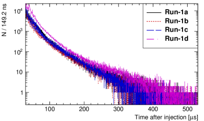
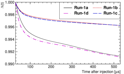
Figure 14: Muon losses measured for the Run-1a (black), Run-1b (red or dark grey), Run-1c (blue or medium grey) and Run-1d (magenta or light grey) data subsets. Left: The number of triple coincidences, as measured by the selection criteria described in the text. Right: The correction function $\Lambda(t)$. The value of $\Lambda(t)$ is set to 1 at the fit start time, which is approximately $30\text{\,}\mathrm{\SIUnitSymbolMicro s}$. The two upper curves correspond to the Run-1b and Run-1c datasets, while the two lower curves correspond to Run-1a and Run-1d (see text).

Not all muons remain stored throughout their lifetime in the storage ring; a fraction of them exit the storage ring after striking collimators or other obstacles. The resulting energy loss, which shifts the energy of a muon below the storage ring momentum acceptance range ($\pm$0.15% of 3.1 GeV/c), dominates the beam loss mechanisms. A loss of muons leads to a time dependence of the normalization factor $N$ in the decay time spectrum of Eq. 2 and requires correction.

A fraction of these lost muons will pass through one or more calorimeters, depositing in each an energy typical of a MIP of about $170$ MeV. The lost muons passing through multiple calorimeters have a time of flight between successive calorimeters of 6.15 ns. These two characteristics allow identification of lost muons and a measurement of the loss rate up to an overall acceptance factor [45, 46]. As a balance between statistics and accidental contamination, we require that the lost muon candidates cross at least three calorimeters. The remaining, minimal amount of accidental contamination in the triple coincidence sample can be corrected for on average by searching for coincidences in nearby time-of-flight windows. Figure 14 (left) shows the corrected time spectrum of lost muons for each dataset taken during Run-1.

For the two calorimeters that each sit behind a tracking station, muons can be easily identified by comparing the momentum ($p$) and the energy ($E$) measured by the two detectors, as shown in Fig. 15. Thus, as an alternative method to the one described above, lost muon candidates can be selected with the following approach. First, we apply a cut on the $E/p$ ratio of the detected particles. We then build a likelihood function based on the measurements made by the two calorimeters. This function includes information regarding the deposited energy, position distribution, and time of flight with respect to temporally adjacent calorimeters. This likelihood function allows selection of muons in all 24 calorimeters, providing a muon loss spectrum that is totally compatible with the one identified by the method described above.

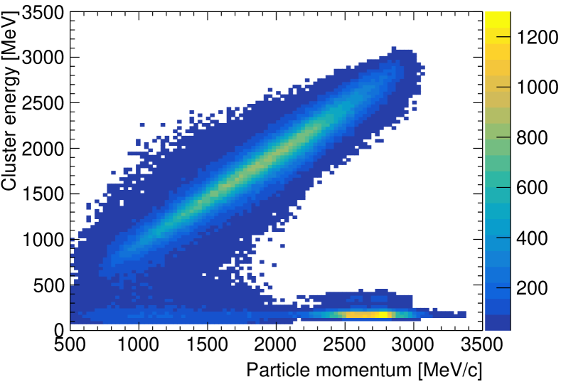
Figure 15: Cluster energy versus particle momentum for tracks crossing a tracker station and hitting the following calorimeters. The positron line, along the diagonal, and the muon peak, with deposited energy of 170 MeV and particle momentum slightly lower than 3 GeV/c, are clearly visible. Scattered muons can also have a lower momentum, while still depositing the energy of a Minimum Ionizing Particle. Note that the tracker geometrical acceptance decreases below $p=1$ GeV/c due to the particle curvature.

The presence of the muon loss spectrum $L(t)$ modifies the simple exponential decay by introducing a multiplicative correction function:

$$\Lambda(t)=1-K_{\rm loss}\int_{0}^{t}e^{t^{\prime}/\gamma\tau}L(t^{\prime})dt^{\prime}.$$ (25)

Reference [46] presents a derivation of this correction function. The normalization parameter $K_{\rm loss}$, related to the calorimeter geometrical acceptance and to the selection efficiency, is determined by the $\omega_{a}^{m}$ fit. Figure 14 shows the typical distortion of the simple exponential introduced by these lost muons: the effect is concentrated in the first tens of microseconds and the total loss rate, integrated over the fill, varies between $3-4$ per mille for datasets 1b and 1c, in which the ESQs operated at a high tune value $n=0.120$ (see Tab. 1), and $7-8$ per mille for datasets 1a and 1d, for which $n=0.108$.

Reference [3] discusses the small correction to $\omega_{a}^{m}$ that can result if the lost muon sample has a different phase content than the muon decay sample used in the fits.

VI.2 Beam dynamics and detector acceptance-based fit model

Four fundamental frequencies, first introduced in Sec. I, can fully describe the dynamics of the muon ensemble: the anomalous precession frequency, $f_{a}=\omega_{a}^{m}/(2\pi)$; the cyclotron frequency, $f_{c}$; the horizontal betatron frequency, $f_{x}$; and the vertical betatron frequency, $f_{y}$. Together with their harmonics and admixtures, these frequencies account for each frequency observed in Fig. 13. Ref. [45] provides a physical description of these frequency combinations. The fitting model

$$F(t)=N_{0}\cdot N_{x}(t)\cdot N_{y}(t)\cdot\Lambda(t)\cdot e^{-t/\gamma\tau_{\mu}}\cdot$$

$$\left[1+A_{0}\cdot A_{x}(t)\cdot\cos{(\omega_{a}^{m}t+\phi_{0}\cdot\phi_{x}(t))}\right]$$ (26)

modifies the basic rate model of Eq. 2 to incorporate the effects of detector acceptance and beam dynamics. The parameter $N_{0}$ is the overall normalization, $\Lambda(t)$ is the muon loss correction given in Sec. VI.1, $A_{0}$ is the decay asymmetry, and $\phi_{0}$ is the initial average spin precession phase. The terms $N_{x}$, $N_{y}$, $A_{x}$, and $\phi_{x}$ describe the interplay between calorimeter acceptance and beam dynamics that affect the overall rate, the average asymmetry and the average phase. These functions are defined as

$$N_{x} (t)={} 1 {}+{} e^{-1t/\tau_{\text{CBO}}} A_{N,x,1,1} \cos(1\omega_{\text{CBO}} t+\phi_{N,x,1,1} )$$

$${}+{} e^{-2t/\tau_{\text{CBO}}} A_{N,x,2,2} \cos(2\omega_{\text{CBO}} t+\phi_{N,x,2,2} )$$ , (27)

$$N_{y} (t)={} 1 {}+{} e^{-1t/\tau_{y}} A_{N,y,1,1} \cos(1\omega_{y} t+\phi_{N,y,1,1} )$$

$${}+{} e^{-2t/\tau_{y}} A_{N,y,2,2} \cos(1\omega_{\text{VW}} t+\phi_{N,y,2,2} )$$ , (28)

$$A_{x} (t)={} 1 {}+{} e^{-1t/\tau_{\text{CBO}}} A_{A,x,1,1} \cos(1\omega_{\text{CBO}} t+\phi_{A,x,1,1} )$$ , (29)

$$\phi_{x} (t)={} 1 {}+{} e^{-1t/\tau_{\text{CBO}}} A_{\phi,x,1,1} \cos(1\omega_{\text{CBO}} t+\phi_{\phi,x,1,1} )$$ . (30)

For the case of $N_{x}(t)$ in Eq. 27, the parameters of the form $A_{N,x,i,j}$ and $\phi_{N,x,i,j}$ correspond to the effect of the $i^{\rm th}$ moment of the radial ($x$) beam distribution at the $j^{\rm th}$ multiple of the fundamental frequency (for $N_{x}(t)$, $\omega_{\rm CBO}$) on the rate normalization $N$ [45]. Analogous parameters in Eqs. 28–30 model the modulation of the average asymmetry $A$ and phase $\phi$, as well as the effect of moments of the vertical ($y$) beam distribution. Some analysis groups employ small variations of the higher order terms of the beam dynamics modeling in their fitting function compared to the model presented here, providing a valuable cross check. Other model variations include an additive rather than multiplicative correction to the phase term. Those terms couple very weakly to $\omega_{a}^{m}$ with the statistics of the Run-1 datasets, and these model variations have negligible effect.

The damaged high voltage resistors for the electrostatic ESQs in Run-1 (see Sec. II.1) add one further modeling requirement by necessitating a time-dependent CBO frequency. The straw tracker system measures this dependence directly in each subset of Run-1, and the substitution

$$\omega_{\rm CBO}\cdot t\rightarrow\omega_{\rm CBO}\cdot t+A_{1}e^{-t/\tau_{1}}+A_{2}e^{-t/\tau_{2}}$$ (31)

from integration of the instantaneous frequency model replaces the static frequency term in Eqs. 27–30. The parameter $\omega_{\rm CBO}$ floats freely in the fits, while the time variations remain fixed. The trackers provide the exponential parameters of the time dependence, with short and long lifetimes of order $8\text{\,}\mathrm{\SIUnitSymbolMicro s}$ and $80\text{\,}\mathrm{\SIUnitSymbolMicro s}$, respectively. The integrated form captures both the frequency shift and the accumulated phase shift.

In a weak-focusing storage ring, the vertical oscillation ($\omega_{y}$) and horizontal CBO frequencies satisfy the relationship

$$\omega_{y}(t)=\kappa_{y}\cdot\omega_{\text{C}BO}(t)\left(\frac{2\omega_{c}}{\kappa_{y}\cdot\omega_{\text{C}BO}(t)}-1\right)^{1/2}.$$ (32)

For continuous ESQ plates generating a perfectly linear field around the ring $\kappa_{y}=1$, but the partial coverage and field non-linearities distort the relationship between $\omega_{y}$ and $\omega_{\text{C}BO}$. A shift in $\kappa_{y}$ at the $1\%$ level reflects these distortions. The correction parameter $\kappa_{y}$ floats in the fit, and the best fit values agree with beam motion measurements with the straw tracking system. The vertical oscillation frequency aliases down to the vertical width frequency via

$$\omega_{\text{V}W}(t)=\omega_{c}-2\omega_{y}(t).$$ (33)

A similar function models the time series obtained with the integrated energy analysis, though two additional effects require further modeling. These effects, described below, require a multiplicative correction to the normalization in a manner analogous to the muon loss correction $\Lambda(t)$.

VI.2.1 Electronics ringing term

As discussed in Sec. IV.3, for the integrated energy approach the average of the time bins in the pedestal window provides an estimate for the pedestal in the signal bin. Consequently, any change in the slope of the pedestal over the window introduces a bias.

The dominant source of pedestal bias arises from electronics ringing, with a period comparable to the pedestal window, following the $t=0$ injection flash. The average difference between (a) the time samples with no pulse above threshold, and (b) the pedestal estimates for that sample, provides an estimate of the ringing as a function of time into the fill. This ringing term and an associated normalization parameter are then incorporated in the fit function in the same manner as the muon loss term. The anomalous precession frequency $\omega_{a}^{m}$ changes by only $\mathcal{O}(10~{}\text{ppb})$ when including or excluding this term.

VI.2.2 Vertical drift term

As discussed in Ref. [3], the vertical distribution of stored muons for Run-1 changes slightly over the fill because of a time dependence of the ESQ voltages on two of the 32 plates. Consequently, the positron acceptance at the top and bottom of the calorimeters will change, and introduce further time dependence of the fit normalization. With the low positron energy threshold for the integrated energy analysis, and thus a correspondingly broader vertical distribution at the calorimeter, this method becomes sensitive to the drift. The time distributions of the energy deposited in the three upper rows of crystals in the calorimeter show a gradual decrease in deposited energy as a function of time into the fill, while those in the lower rows of crystals show an increase. The magnitude of the effect varies systematically with row – maximal at the outermost rows and smallest in the central rows.

Tracking-based studies indicate that the drift and width changes occur with the similar time dependences. By carrying the measured dependence from the crystal row studies through to the normalization, we obtain a data-driven correction to the normalization, analogous to the lost muon correction.

In addition, we investigate the possible effects of vertical drift on the asymmetry parameter. The measured asymmetry correlates with vertical position through acceptance effects, and therefore a change in vertical profile can also change the asymmetry as a function of the fill time.

Excluding versus including the vertical drift correction in the fit shifts the extracted value of the anomalous precession frequency $\omega_{a}^{m}$ by $\mathcal{O}(100~{}\text{ppb})$. The normalization term dominates this shift, with the effect from the correction to the asymmetry parameter entering at least an order of magnitude smaller.

VI.3 Software blinding of $\omega_{a}^{m}$

Each analysis group introduces an independent blinding of $\omega_{a}^{m}$ at the software level within their fits, which prevents unconscious biasing towards the central value of any particular group. This blinding proceeds through the introduction of an offset $\Delta R$, defined as

$$\omega_{a}^{m}(R)=\omega_{\rm ref}[1-(R-\Delta R)\times 10^{-6}],$$ (34)

where the reference frequency $\omega_{\rm ref}=2\pi\times 0.2291~{}\rm{MHz}$. This parameterization expresses $\omega_{a}^{m}$ in terms of the shift $R$ in parts per million (ppm) from the reference frequency, and it introduces the blinded shift between the value used in the fit model and the displayed results. Each analysis group chooses a blinding text phrase, which a standardized package converts to a value of $\Delta R$, keeping the shift itself unknown to the group. An MD5 hash algorithm converts the blinding phrase to four 32-bit seeds for a Mersenne Twister random number generator. Using this seeded generator, the package draws the blinding factor $\Delta R$ from a flat $\pm 24$ ppm distribution with 1 ppm Gaussian tails. This procedure always produces the same blinded shift $\Delta R$ for a given blinding phrase.

Unblinding at the software level proceeded in two stages. The first relative unblinding occurred after each analysis group completed their analysis, including all cross checks and systematic uncertainty evaluation. At that point, all groups adopted a common blinding offset to allow a direct comparison of results. The final common software blinding and the hardware-level blinding were only removed after the final decision to proceed with publication.

VI.4 Parameter determination

All analyses determine the best fit parameters through minimization of the Neyman $\chi^{2}$

$$\chi^{2}=(\mathbf{N}-\mathbf{F})^{T}\mathbf{V}^{-1}(\mathbf{N}-\mathbf{F}),$$ (35)

with the MINUIT numerical minimization package [47] either directly or through the ROOT software package [48]. The vectors $\mathbf{N}=\{N_{i}\}$ and $\mathbf{F}=\{F_{i}\}$ correspond to the measured data time series and corresponding model prediction, respectively, while $V$ represents the data covariance matrix. When correlations may be neglected, analyses employ the simpler form

$$\chi^{2}=\sum_{i}\frac{\left[N_{i}-F(t_{i},\vec{p})\right]^{2}}{\sigma_{i}^{2}}.$$ (36)

The vector $\vec{p}=(N_{0},\tau_{\mu},\omega_{a}^{m},...)$ represents the free parameters described in Sec. VI.2 together with the function $F(t_{i})$. The number of parameters floating in the fit varies with analysis method, the details of the beam dynamics model, and the size of the dataset (which determines sensitivity to the higher-order, lower-amplitude effects from beam dynamics). The number of free parameters ranges from 16 (ratio method) through 27 (integrated energy analysis), with 22 being the typical number for the event-based analyses.

A minimum of 30 to 100 positrons (depending on analysis group) contribute to the weighted sums in even the least populated bins (149.2 ns wide) for the event-based analyses, so a Gaussian approximation to the Poisson distribution works well in estimating uncertainties. Standard error propagation for the asymmetry weighting, and for the corrections for pileup and muon loss also apply. The event-based and ratio analyses have about 4000 degrees of freedom in the fits, while the integrated energy analyses have about 1210. We require that all fits contributing to this work have a reduced $\chi^{2}$ consistent with unity within the expected standard deviation of 0.02 (0.04) for the event-based (integrated energy) analyses – a necessary but not sufficient condition for an unbiased determination of $\omega_{a}^{m}$. In addition, all fits had to exhibit a structure-free residual distribution in both time and frequency domains.

Parameter	Fit result	Parameter	Fit result
blinded $R$ (ppm)	$-16.01\pm 0.68$	$\tau_{y}$ ($\mathrm{\SIUnitSymbolMicro s}$)	$168\pm 98$
$N_{0}$	$(7249.8\pm 3.5)\times 10^{3}$	$A_{N,y,2,2}$	$0.00039\pm 0.00022$
$\gamma\tau_{\mu}$ ($\mathrm{\SIUnitSymbolMicro s}$)	$64.4478\pm 0.0023$	$\phi_{N,y,2,2}$	$2.10\pm 0.65$
$A_{0}$	$0.355193\pm 0.000021$	$A_{N,x,2,2}$	$0.000198\pm 0.000059$
$\phi_{0}$	$2.07519\pm 0.00013$	$\phi_{N,x,2,2}$	$-3.35\pm 0.30$
$\omega_{\text{CBO}}$ (s-1)	$2.33593\pm 0.00030$	$A_{A,x,1,1}$	$0.00059\pm 0.00014$
$\tau_{\text{CBO}}$ ($\mathrm{\SIUnitSymbolMicro s}$)	$190\pm 11$	$\phi_{A,x,1,1}$	$-0.38\pm 0.24$
$A_{N,x,1,1}$	$0.003237\pm 0.000097$	$A_{\phi,x,1,1}$	$0.000108\pm 0.000072$
$\phi_{N,x,1,1}$	$-6.081\pm 0.029$	$\phi_{\phi,x,1,1}$	$-3.19\pm 0.66$
$K_{\rm loss}$	$0.00903\pm 0.00036$	$A_{N,y,1,1}$	$-0.000082\pm 0.000046$
$\kappa_{y}$	$1.01398\pm 0.00063$	$\phi_{N,y,1,1}$	$-5.98\pm 0.58$

Table 2: The (blinded) fit results for the asymmetry-weighted event analysis for the Run-1d dataset. The fit used the model and parameters described in Equations 25 through 30 and Eq. 34.

Table 2 presents the results of a fit to the Run-1d data, the subset with the largest statistics, for an analysis using the model exactly as presented above. Figure 16 shows both the result of the above fit overlaid on the precession data and the FFT of the residual distribution. With the full beam dynamics model incorporated into the fit, this residual distribution no longer exhibits any characteristic structure.

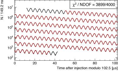
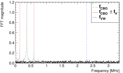
Figure 16: Left: the overlay of the fit described in the text on the Run-1d precession data. Right: the FFT of the time distribution of residuals to that fit (black), which shows no remaining characteristic frequencies in the spectrum. For contrast, the residuals of the 5-parameter fit with no beam modeling are also shown (light gray), which helps to highlight the excellent performance of the fit including the modeling.

Table 3 shows the correlation coefficients for the fundamental five parameters of Eq. 2 and the most significant beam dynamics component, while Appendix A provides the full correlation matrix. The strongest correlation of $\omega_{a}^{m}$ ($R$) in the fits occurs with the average initial precession phase, $\phi_{0}$, analogous to the slope-intercept correlation in a linear fit. It has only small correlations with all other parameters. While the correlations of $\omega_{a}^{m}$ with the CBO-related parameters are small, the strength of the leading terms in the CBO model (reflected by the significance of the signal in the fit) requires that we include these parameters in the fit. If we drop all CBO-related effects in the model, $\omega_{a}^{m}$ shifts significantly (of order 100 ppb). Suppose we include the $N_{x,1,1}$ and $A_{x,1,1}$-related terms in Eqs. 27 and 29, which correspond to the main peak at the frequency $f_{\rm CBO}$ in the residuals to the five-parameter fit (Fig. 13). The remaining terms in the CBO modeling affect $\omega_{a}^{m}$ by at most 20 ppb.

The correlation matrix also shows a strong correlation among the overall normalization and the two parameters controlling a slow variation over the time of the fill – the lifetime parameter and the muon loss normalization. Increasing the muon lifetime, or the fraction of lost muons, the overall normalization increases.

Because of aliasing of the radial oscillations at positions 180^∘ apart in the ring, the effects of CBO in one calorimeter tend to compensate for the effects in the calorimeter directly across the ring. To leading order, and neglecting decoherence, the sum of data from all calorimeters provides a complete cancellation that is independent of variation in the radial betatron frequency. Small differences in the calorimeter acceptances result in a residual effect. Nevertheless, summing the data over all calorimeters significantly suppresses the effects of the CBO in the fits. Excluding the CBO terms in the fit function in fits to individual calorimeters results in shifts in $\omega_{a}^{m}$ an order of magnitude larger than those observed for fits to data summed over all calorimeters.

	$R$	$N_{0}$	$\gamma\tau_{\mu}$	$A_{0}$	$\phi_{0}$	$\omega_{\text{CBO}}$	$\tau_{\text{CBO}}$	$A_{N,x,1,1}$	$\phi_{N,x,1,1}$	$K_{\rm loss}$
$R$	1.00	-0.01	-0.00	0.00	-0.87	0.01	0.02	-0.03	-0.02	-0.01
$N_{0}$		1.00	0.86	-0.03	0.01	-0.00	-0.03	0.05	0.00	1.00
$\gamma\tau_{\mu}$			1.00	-0.02	0.00	-0.00	-0.02	0.03	0.00	0.89
$A_{0}$				1.00	-0.01	0.01	-0.01	0.01	-0.02	-0.04
$\phi_{0}$					1.00	-0.02	-0.03	0.04	0.02	0.01
$\omega_{\text{CBO}}$						1.00	-0.03	0.03	-0.92	-0.00
$\tau_{\text{CBO}}$							1.00	-0.92	0.03	-0.03
$A_{N,x,1,1}$								1.00	-0.03	0.04
$\phi_{N,x,1,1}$									1.00	0.00
$K_{\rm loss}$										1.00

Table 3: The correlation matrix among the main parameters (full matrix in Appendix) from the fit whose results are presented in Table 2. The parameters are defined in Equations 25 through 30 and Eq. 34. For purposes of display, the elements below the diagonal for this symmetric matrix have been not been included.

Table 4 presents the values for $R$ from each of the 11 fits to each of the four datasets. Also provided are the simple statistical weighted averages over the four datasets for a higher precision comparison. Note that the simple averages presented here do not incorporate the small shifts in the magnetic field value and changes in the beam dynamics corrections that vary set by set. The averages are only provided to allow assessment of the level of agreement among the results from the different analysis methods. Reference [1] incorporates all necessary changes for a dataset by dataset comparison of the anomalous magnetic moment. The values presented here also have the hardware blinding and a common software blinding still applied.

		$R$ [ppm] for each dataset					Naive $R$
Recon.	Method	Pileup	Run-1a	Run-1b	Run-1c	Run-1d	average [ppm]
global	A	empirical	-82.98 $\pm$ 1.21	-81.70 $\pm$ 1.03	-82.30 $\pm$ 0.82	-82.34 $\pm$ 0.68	-82.30 $\pm$ 0.43
local	A	shadow	-83.23 $\pm$ 1.20	-81.77 $\pm$ 1.02	-82.35 $\pm$ 0.82	-82.48 $\pm$ 0.67	-82.41 $\pm$ 0.43
local	A	shadow	-83.17 $\pm$ 1.21	-81.84 $\pm$ 1.03	-82.50 $\pm$ 0.83	-82.45 $\pm$ 0.68	-82.44 $\pm$ 0.44
local	A	pdf	-83.39 $\pm$ 1.22	-81.72 $\pm$ 1.04	-82.32 $\pm$ 0.83	-82.42 $\pm$ 0.68	-82.39 $\pm$ 0.44
local	T	shadow	-83.55 $\pm$ 1.36	-81.80 $\pm$ 1.16	-82.67 $\pm$ 0.93	-82.45 $\pm$ 0.76	-82.54 $\pm$ 0.49
global	T	empirical	-82.96 $\pm$ 1.34	-81.96 $\pm$ 1.14	-82.77 $\pm$ 0.91	-82.47 $\pm$ 0.75	-82.52 $\pm$ 0.48
local	T	shadow	-83.64 $\pm$ 1.33	-81.83 $\pm$ 1.12	-82.64 $\pm$ 0.91	-82.63 $\pm$ 0.74	-82.62 $\pm$ 0.48
local	T	shadow	-83.49 $\pm$ 1.34	-81.75 $\pm$ 1.13	-82.64 $\pm$ 0.91	-82.42 $\pm$ 0.75	-82.50 $\pm$ 0.48
local	T	pdf	-83.37 $\pm$ 1.33	-81.76 $\pm$ 1.13	-82.65 $\pm$ 0.91	-82.47 $\pm$ 0.74	-82.51 $\pm$ 0.48
local	R	shadow	-83.72 $\pm$ 1.36	-81.96 $\pm$ 1.16	-82.67 $\pm$ 0.93	-82.52 $\pm$ 0.76	-82.62 $\pm$ 0.49
n/a	Q	n/a	-83.96 $\pm$ 2.07	-79.70 $\pm$ 1.76	-81.03 $\pm$ 1.45	-82.74 $\pm$ 1.29	-81.82 $\pm$ 0.78

Table 4: The unblinded $\omega_{a}^{m}$ fit results, in terms of the parameter $R$, from all analyses efforts for the four sets, as well as the naive weighted average of the results for a more stringent comparison among the different analyses. The “Recon.” column indicates whether the local or global reconstruction methods (see Sec. IV) provided the positron candidates. Under the “Method” column, T corresponds to an event-based analysis with unit weighting (equivalent to a simple energy threshold), A corresponds to an asymmetry-weighted event-based analysis, R corresponds to the ratio method applied to the unit-weighted event-based sample, and Q corresponds to the integrated energy (akin to a charge integration) analysis.

VI.5 Corrections to and comparisons of $\omega_{a}^{m}$

Table 5 shows the expected level of correlations among the different analysis and reconstruction types. Statistically-allowed differences arise, for example, from differences in the local and global reconstruction, in parameter choices within the local reconstruction, in the weighting of positron events in different analysis methods, in different positron energy thresholds and fit start time choices, in binning differences, and in different choices in the lost muon selection algorithms, among other effects. We determined these correlations from $\sim 10^{3}$ Monte Carlo simulation trials that incorporate the major reconstruction and analysis differences that drive the range of allowed fluctuations. Given these correlation coefficients, the expression

$$\Delta\sigma_{12}=\sqrt{\sigma_{1}^{2}+\sigma_{2}^{2}-2\rho\sigma_{1}\sigma_{2}}$$ (37)

provides the allowed $1\sigma$ statistical deviation $\Delta\sigma_{12}$ between fit values for $\omega_{a}^{m}$ from two different analyses. The parameters $\sigma_{1}$ and $\sigma_{2}$ correspond to the statistical uncertainties of the two measurements, while $\rho$ corresponds to the correlation between the two analyses.

The different analyses are strongly correlated and it is known ([49, 50]) that, for two positively correlated results, the variance of the combination has a maximum for

$$\rho_{\text{crit}}=\mbox{min}(\sigma_{1}/\sigma_{2})/\mbox{max}(\sigma_{1}/\sigma_{2}),$$ (38)

while it drops to zero when the correlation moves from $\rho_{crit}$ to 1. Because of this, particular care is required in combining the different analyses, as described in Sec. VIII.

The pulls of different R measurements (see Tab. 4) on the same dataset distribute approximately as a unit Gaussian. The integrated energy measurements show a moderate systematic shift with respect to the event based measurements, and these correlated shifts coupled with the O(200 ppb) difference in the corrections for the damaged quad resistor largely explain the differences of stop times in these two categories of measurements.

Recon./Method	global/T	global/A	local/T	local/A	local/R	Q
global/T	1.00	0.91	0.95	0.91	0.95	0.51
global/A		1.00	0.90	0.99	0.90	0.58
local/T			1.00	0.91	1.00	0.51
local/A				1.00	0.90	0.57
local/R					1.00	0.50
Q						1.00

Table 5: The statistical correlations found from Monte Carlo trials for the different types of $\omega_{a}^{m}$ analyses and positron reconstruction methods. The reconstruction and analysis shorthands are defined in Tab. 4.

VI.6 Internal consistency

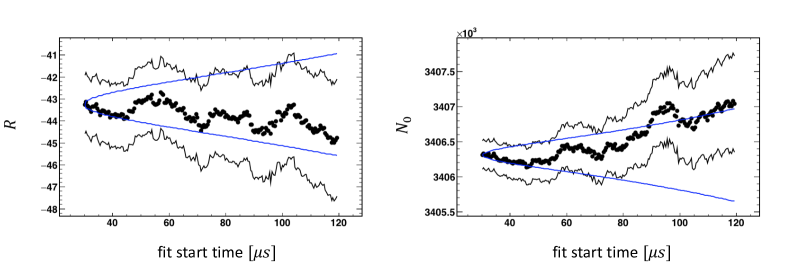
Figure 17: The $R$ (left) and $N_{0}$ (right) parameters from a scan of the full fit to the Run-1a data subset over the fit start time. The black curves above and below the data points indicate the full statistical error on $R$ or $N_{0}$ from the fits. The one standard deviation bands (blue) show the allowed statistical variation of any given point relative to the nominal fit (starting point), and take into account the highly correlated statistics between those two points. No scans show any systematic trends away from the statistically consistent region, nor any oscillation at the $\omega_{a}^{m}$ period – typical indicators of data mismodeling. The trend near the one standard deviation band simply indicates that data from the earliest fit times drive that statistically compatible shift.

To add further confidence in our data model and resulting fit, and to probe for residual systematic effects, a number of consistency checks have been performed. The fit results should remain stable with respect to the fit start time. Later start times reduce potential bias from residual effects that are pronounced at early times, such as cyclotron motion, effects from the dynamics of the stored beam, positron pileup and gain changes related to the injection process. Improper modeling of slow effects, such as those due to gain stability or muon loss, would appear as an oscillation of the extracted value of $\omega_{a}^{m}$ at the period of the anomalous precession itself. Stability of the fitted $\omega_{a}^{m}$ as a function of start time indicates that these effects are controlled to within the allowed statistical variation given the small change in statistics relative to the nominal start time. Figure 17 shows the two parameters $R$ (see Eq. 34) and $N_{0}$ from a fitting start time scan for one analysis. Both these combined scans and the individual subset scans show excellent $\omega_{a}^{m}$ stability. Most of the data remains common to each point in the start time scan, significantly correlating the parameter values for each point in the start time scan. The scans therefore reveal trends, as opposed to exhibiting the statistical scatter of statistically independent samples. The maximum excursion in $N_{0}$ at a start time of $\sim$$90\text{\,}\mathrm{\SIUnitSymbolMicro s}$ means that $N_{0}$ from that fit agrees with $N_{0}$ from the nominal start time at $\sim 1.5$ standard deviations given the change in statistics.

Figure 18: The $R$ parameters from fits to the Run-1c dataset by individual calorimeter, relative to their average.

We have also fit for $\omega_{a}^{m}$ using the data in each of the 24 individual calorimeter stations (Fig. 18). As noted earlier, the data from an individual station have a significantly more pronounced CBO motion than the combined data. Thus, we can use the individual fits as sensitive probes to evaluate our beam dynamics model. Residual effects from the cyclotron motion can also induce a bias of $\omega_{a}^{m}$ as a function of position around the storage ring. The value of $\omega_{a}^{m}$ remains stable as a function of calorimeter station, indicating proper accounting for these effects.

Extracting $\omega_{a}^{m}$ as a function of positron energy probes systematic effects that depend on positron energy, such as positron pileup and instability in the energy scale. The energy scans show no systematic dependence of $\omega_{a}^{m}$ on energy. The energy scans do show an unphysical variation of the muon loss normalization parameter $K_{\rm loss}$. A number of sources can contribute to such an effect, such as a residual gain miscalibration on the order of a few parts per $10^{4}$, an overall drift in positron or lost muon acceptance as a function of time into the fill, or residual issues with the pileup correction. The pileup correction, for example, becomes more pronounced at larger positron energies. The different sources can shift $\omega_{a}^{m}$ in different directions, so we do not apply an overall correction to the central value of $\omega_{a}^{m}$. The systematic uncertainty receives a contribution from this residual early-to-late effect, as discussed in the next section.

Other cross checks include fits for $\omega_{a}^{m}$ versus run number, time of day, the bunch number within the supercycle of 16 fills, calorimeter column and row number, none of which show any systematic trend.

VII Systematic uncertainties

The known potential systematic effects and their possible biasing of the extracted $\omega_{a}^{m}$ value were evaluated for each analysis. For all datasets and analyses, the statistical uncertainties exceeded the systematic uncertainties by one to two orders of magnitude. The dominant systematic uncertainties arise from uncertainties in the calorimeter gain corrections (Sec. V.1), in multi-positron pileup (Sec. V.2), in the beam dynamics model (Sec. VI.2), and from the unknown source of the unphysical energy dependence of the lost muon normalization parameter. This section will discuss the methods used to estimate these uncertainties. While we have investigated many other sources of potential bias, the estimated systematic uncertainty on $\omega_{a}^{m}$ fell below 10 ppb and has negligible effect on the result. Table 7 summarizes the systematic uncertainty on the extracted $\omega_{a}^{m}$ value for each dataset and for each source of systematic uncertainty. The following section describes the method used to combine the different analyses and thus to arrive at this summary table.

VII.1 Detector gain corrections

Short term and in-fill gain corrections (Sec. V.1) remove the energy scale variation in each calorimeter channel as a function of time into the muon fill. The statistical uncertainties of the gain functions’ best-fit amplitudes and characteristic time constants, which are both typically between 10 and 20%, introduce a systematic uncertainty on the extracted $\omega_{a}^{m}$ value. The long-term gain correction, on the other hand, does not pose a systematic bias to the extracted $\omega_{a}^{m}$ value because it is constant across each muon fill.

A sweep of the amplitude of the exponential gain correction function through a common multiplicative scaling applied to all calorimeter channels provides an assessment of the collective sensitivity of $\omega_{a}^{m}$ to the in-fill correction and to the short term correction. Figure 19 illustrates the sensitivity obtained for different methods from two analysis groups. The average uncertainty of the amplitudes for all crystal corrections provides the range that determines the uncertainty estimate for $\omega_{a}^{m}$ given the measured sensitivity. The determination of the uncertainty from the time constants in the exponential form employed an analogous procedure.

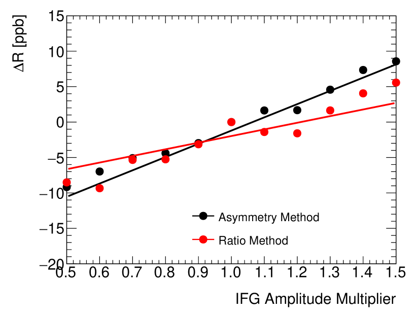
Figure 19: Sensitivity of $\omega_{a}^{m}$ to the amplitude of the in-fill gain correction for one of the Asymmetry-weighted analyses (black) and the Ratio method analysis (red). The precession frequency changes by $18.8\,$ ppb and $9.4\,$ ppb, respectively, for a variation of the amplitude scaling factor that corresponds to one standard deviation in its average uncertainty. As described in Sec. III.4, the ratio method is less sensitive to these “slow effects”.

We find systematic uncertainties on $\omega_{a}^{m}$ from the in-fill and short term gain correction of order of 10 and 1 ppb, respectively, across all data subsets.

VII.2 Multi-positron pileup

The sources of systematic uncertainty on $\omega_{a}^{m}$ related to multi-positron pileup depend on the reconstruction (Sec. IV) and correction (Sec. V.2) approaches used. For instance, the global-fitting approach to reconstruction significantly reduces the amount of pileup, leading to a smaller correction and in turn a smaller systematic uncertainty on $\omega_{a}^{m}$. We estimate an uncertainty due to pileup under 5 ppb across the datasets for the analysis that used this reconstruction approach. This subsection therefore focuses on the remaining analyses that used the local-fitting approach to reconstruction, along with either the shadow-window or probability-density-function approaches to the pileup correction.

In these analyses, the dominant systematic uncertainties on $\omega_{a}^{m}$ arise from uncertainties in the pileup correction’s amplitude and phase. A scaling procedure, like the one used to assess the gain correction amplitudes, provides the sensitivity of the extracted value of $\omega_{a}^{m}$ to the amplitude.

To determine the uncertainty in the amplitude itself, the analysis groups use one of two methods. The first method tabulates the $\chi^{2}$ from the full fit as a function of the scaled pileup amplitude. A quadratic interpolation to the $\chi^{2}$ distribution near its minimum then provides the amplitude uncertainty via $\Delta\chi^{2}=\pm 1$. The second method uses agreement between the estimated pileup distribution and the data in the energy spectrum in the non-physical region above 3.5 GeV (Fig. 12) to estimate the uncertainty.

To estimate the systematic uncertainty from the phase, some analyses shift the correction in time to evaluate the sensitivity of $\omega_{a}^{m}$ to the phase. We combine this sensitivity with the ambiguity in the pileup time estimate in each method to obtain the systematic uncertainty. Other analyses that use the shadow-window approach vary the time (and energy) models in Eqs. 17 and 18. The resulting change in the extracted $\omega_{a}^{m}$ value yields the uncertainty estimate.

For analyses using the local-fitting approach to reconstruction, the total systematic uncertainty on $\omega_{a}^{m}$ from the pileup correction ranges from about 30 to 40 ppb across the datasets.

VII.3 Beam dynamics

The fit function accounts for the imprint of beam dynamics on the calorimeter data through the terms in Eqs. 26–31, and the uncertainty in that modeling leads to a systematic uncertainty on the extracted $\omega_{a}^{m}$ value. The dominant modeling uncertainties come from the time-dependent CBO frequency ($\omega_{\text{CBO}}(t)$) and the CBO decoherence envelope ($e^{-t/\tau_{\text{CBO}}}$). Information provided by the tracking system determines the time dependence of the CBO frequency caused by the damaged ESQ resistor. The difference in the parameterization obtained separately from the two tracker stations provides the estimate of the uncertainty on $\omega_{\text{CBO}}$. We find an uncertainty of order 10 ppb across all datasets and analyses.

The tracker data also constrain the uncertainty from the modeling of time dependence of the CBO envelope. The data show consistency with an exponential behavior for the decoherence of the betatron oscillations at the current level of precision. However, beam dynamics simulations of the $g-2$ and other storage rings indicate that the betatron oscillations within the stored beam can re-cohere. Fits using the two alternate CBO envelope models

$$e^{-t/\tau_{\text{CBO}}}+B,$$ (39)

$$e^{-t/\tau_{\text{CBO}}}\left[1+C\cdot\cos\left(\omega_{C}t+\phi_{C}\right)\right],$$ (40)

where $B$, $C$, $\omega_{C}$, and $\phi_{C}$ are additional fit parameters that we either float freely in the fit or fix to the values determined from the tracker data, bound the sensitivity of $\omega_{a}^{m}$ to the envelope. Note that the model in Eq. 40 is itself motivated by beam-dynamics simulations.

Additionally, each envelope model assumes a common $\tau_{\text{CBO}}$ for the CBO modulation of the normalization, asymmetry, and phase terms in Eq. 26. However, simulations suggest that these time constants could vary by as much as 50 %. The largest shift in $\omega_{a}^{m}$ observed under variation of each of these time constants by up to 50% provided an additional contribution to the systematic uncertainty. Depending upon the analysis technique and data subset, this uncertainty ranged from 10 to 50 ppb.

The interplay between the three classes of beam dynamics parameters discussed in this section likely correlates them. We therefore conservatively combine these three contributions linearly to arrive at the total systematic uncertainty on $\omega_{a}^{m}$ from the beam dynamics modeling. For the average of the asymmetry-weighted event-based analyses presented below, this uncertainty ranges from 30 to 50 ppb across the data subsets.

VII.4 Residual early-to-late effect

The introduction of an ad hoc time-dependent correction to the energy scale can eliminate the unphysical positron energy dependence of the muon loss rate (see Sec. VI.6). The scale of the required correction typically amounts to a few $\times 10^{-4}$, depending upon the reconstruction method and dataset. A small time-dependent acceptance variation can similarly ameliorate this effect, but with a shift of $\omega_{a}^{m}$ in the opposite direction. The source of the effect remains under investigation. For this analysis, we do not apply an overall correction, but we assign a systematic uncertainty on $\omega_{a}^{m}$ of $\simeq 20$ ppb based on the shift of its central value upon application of one of the corrections.

VII.5 Additional systematic effects

We have evaluated many other potential sources of bias on $\omega_{a}^{m}$, and find their effects to be under 10 ppb on the final Run-1 $a_{\mu}$ average, and therefore negligible for the result from this Run-1 dataset. Two of these effects of note that have been considered include muon loss (see Sec. VI.1) and time randomization (see Sec. III.5).

The contribution of the muon loss correction has been evaluated by modifying the shape of the lost muons function $L(t)$ in Eq. 25 according to different selection criteria.

Tests of the stability of the time randomization procedure include variation of the binning size in time, incorporating the spread of cyclotron periods (from the spread of stored muon energies) into the time randomization process, and by comparing the time randomization for a cluster-by-cluster versus a fill-by-fill basis. Variation of $\omega_{a}^{m}$ in these tests remained well below 10 ppb. To minimize the statistical fluctuations introduced by the minimization procedure, each analysis effort reanalyzed and refit the data using many random number seeds. The quoted uncertainty reflects the residual uncertainty from the finite number of seeds employed.

Both these contributions have an effect of less than 10 ppb on the $a_{\mu}$ average.

Other items investigated but below threshold for significant discussion include studies of $\chi^{2}$ vs likelihood fitting, the extracted cluster time of the reconstructed positron candidates, the short time gain correction parameters, biases in the reconstructed time and energy in the empirical pileup estimation method, the lost muon selection criteria and the master clock stabilility. In all, the full list of investigated uncertainty categories included thirty seven separate categories. Some of these were likely highly correlated and were combined linearly to obtain the final categories above, or, like those listed here, were found to be negligible.

VIII Analysis combination

Ideally, combination of the $\omega_{a}^{m}$ results for each of the four data subsets from each of the eleven analyses would proceed through a best linear unbiased estimator (BLUE) averaging procedure. For example, one could minimize

$$\chi^{2}=\bm{\Delta_{\omega}}^{T}\bm{C}^{-1}\bm{\Delta_{\omega}},$$ (41)

where $\Delta_{\omega}=\omega_{a,i}-\bar{\omega}_{a}$ is the difference between the i^th measurement and the average $\bar{\omega}_{a}$, and the covariance matrix $\bm{C}$ includes the correlations, statistical and systematic, between the eleven determinations of $\omega_{a}^{m}$. When combined with the magnetic field measurements for each subset, this approach would expand to $11\times 4$ determinations to be averaged.

For the Run-1 sample presented here, the statistical uncertainties dominate the covariance matrix for a given data subset, and the significant statistical correlations among the eleven results for a given dataset pose practical impediments to a well-behaved procedure [49, 50]. In particular, the correlation between different analyses often reaches the “critical value” defined in Equation 38.

Therefore, to correctly compute an average, accurate estimates of the statistical correlations are required. These have been estimated with toy Monte Carlo simulations and have been shown in Tab. 5. Additional systematic uncertainties, due to imperfections of the simulation, have not been estimated and are assumed to be subdominant. The simulation confirms that measurements on the same dataset are all consistent with being “critically correlated”.

As documented in the literature [50, 51], correlations beyond the critical values cause the weights of the less statistically precise measurements to become negative and reduce the uncertainty of the BLUE combination average. We have found that in our conditions the finite precisions of the estimated uncertainties and correlations of the $11\times 4$ measurements of $\omega_{a}^{m}$ make the BLUE procedure highly unstable.

When averaging two measurements that are exactly critically correlated, the BLUE combination has weight = 1 for the most precise result and weight = 0 for the least precise one (see [51]). In the limiting case when two measurements have exactly the same uncertainty and are critically correlated, the two weights are 1/2 each. In our case, it is convenient and reasonable to set all statistical correlations to the critical values, and to set the measurement uncertainties to be exactly the same when using the same method. Under these assumptions, the most precise method, which is the asymmetry-weighted method, gets all the weight, while the other ones get no weight in the combination. This is justified as long as uncorrelated systematic uncertainties are much smaller than the quadratic difference of the total uncertainties between the different methods. In these conditions, there is a negligible benefit in including the other methods’ measurements in the average with the goal of reducing the systematic part of the total uncertainty.

The analyses that use different reconstruction algorithms (local vs. global) are less correlated than the ones using the same reconstruction program (see Tab. 5). Thus we perform a “staged” average of the asymmetry-weighted results for $\omega_{a}^{m}$ by first combining with equal weights all analyses that use the local reconstruction and all analyses that use the global reconstruction and then combining with equal weights the two $\omega_{a}^{m}$ averages of the first stage. The $\omega_{a}^{m}$ results of this simplified procedure have been compared with several other different more complex procedures, all designed to address the issue of the instability of the combination average in case of highly correlated results. Within the context of the BLUE approach, the covariance matrix calculation either caps the correlation coefficients at $\rho_{ij}<\rho^{\rm crit}_{ij}$ or uses Tikhonov regularization [52], which effectively rescales all correlation coefficients down. These calculations assume fully correlated systematic uncertainties across the analyses within each category: gain, muon loss estimation, etc.

For all these approaches, the average of the individual subsets varied by up to 10 ppb in all cases, except one outlier, which varied by 30 ppb. In summary, our results show very good stability over all reasonable average approaches that we have investigated.

Here we present results from the staged averaging approach using only the asymmetry-weighted analyses. This method both makes optimal use of the statistical information and shows the smallest sensitivity to the phase-related correction from the damaged electrostatic quadruples. The statistical uncertainties across the different datasets are uncorrelated, while the systematic uncertainties are strongly correlated, as shown in Table 6.

Table 7 presents the resulting average value of $\omega_{a}^{m}$ foreach the four data subsets. When combining these values, along with their associated magnetic field measurements, to obtain the final Run-1 determination of $a_{\mu}$, these results contribute a total statistical uncertainty of 434 ppb, while their systematic contribution amounts to 56 ppb.

Correlation	1a	1b	1c	1d
1a	1.0000	0.9935	0.9884	0.9812
1b		1.0000	0.9820	0.9935
1c			1.0000	0.9669
1d				1.0000

Table 6: Correlation matrix among different data sets for systematic uncertainties.

Run-1 data set	1a	1b	1c	1d
$\omega_{a}^{m}$/2$\pi$ (s-1)	229080.957	229081.274	229081.134	229081.123
$\Delta$($\omega_{a}^{m}$/2$\pi$) (s-1)	0.277	0.235	0.189	0.155
statistical uncertainty (ppb)	1207	1022	823	675
Gain changes (ppb)	12	9	9	5
Pileup (ppb)	39	42	35	31
CBO (ppb)	42	49	32	35
Time randomization (ppb)	15	12	9	7
Early-to-late effect (ppb)	21	21	22	10
total systematic uncertainty (ppb)	64	70	54	49
total uncertainty (ppb)	1209	1025	825	676

Table 7: The combination result for each data set when using a staged approach.

IX Discussion and conclusion

In this article, we have described the full procedure for the extraction of the muon precession frequency $\omega_{a}^{m}$ for the four datasets collected in 2018. As described in Section II.1, the ESQ and kicker settings were modified over the course of Run-1, in order to optimize the quality of the stored beam. To optimize the determination of $a_{\mu}$, in Ref. [1] we combine the four $\omega_{a}^{m}$ values presented here with corrections and field measurements determined individually for the four datasets. The final value corresponds to the average of those four combined values.

Six analysis groups produced measurements of $\omega_{a}^{m}$ by using two independent reconstruction algorithms, four different histogramming methods and many variants of the procedures used to evaluate the correction factors and to fit the final spectrum. Each analysis was carried out with a different blinding offset. The relative unblinding was performed during a Collaboration Meeting, after all analyses were completed and shown to have an overall agreement.

All analyses show that the error on $\omega_{a}^{m}$, for Run-1, is dominated by the statistical contribution. The systematic uncertainties described in section VII have reached or approached the goal that has been set in the Technical Design Report [33] for the full statistics.

Appendix A Important frequencies and full correlation matrix

Table 8 summarizes the relevant frequencies which characterize the $g-2$ storage ring. The beam related frequencies are evaluated according to the formulae and coincide with the measured values at the $1\%$ level, the difference being due to decoherence effects discussed in Sec. VII.3.

Table 9 provides the full set of correlation coefficients for the fit to the Run-1d dataset described in Section VI.

			n=0.108		n=0.120
Physical frequency	Variable	Expression	Frequency	Period	Frequency	Period
			(MHz)	($\mu$s)	(MHz)	($\mu$s)
Anomalous precession	$f_{\rm a}$	$\frac{e}{2\pi m}a_{\mu}B$	0.229	4.37	0.229	4.37
Cyclotron	$f_{\rm c}$	$\frac{v}{2\pi R_{0}}$	6.71	0.149	6.71	0.149
Horizontal betatron	$f_{\rm x}$	$\sqrt{1-n}\,f_{\rm c}$	6.34	0.158	6.29	0.159
Vertical betatron	$f_{\rm y}$	$\sqrt{n}\,f_{\rm c}$	2.20	0.453	2.32	0.430
Horizontal CBO	$f_{\rm CBO}$	$f_{\rm c}-f_{\rm x}$	0.37	2.68	0.42	2.41
Vertical waist	$f_{\rm VW}$	$f_{\rm c}-2f_{\rm y}$	2.31	0.433	2.07	0.484

Table 8: Frequencies and periods which characterize the $g-2$ storage ring.

	$R$	$N_{0}$	$\gamma\tau_{\mu}$	$A_{0}$	$\phi_{0}$	$\omega_{\text{CBO}}$	$\tau_{\text{CBO}}$	$A_{N,x,1,1}$	$\phi_{N,x,1,1}$	$K_{\rm loss}$	$\kappa_{y}$
$R$	1.00	-0.01	-0.00	0.00	-0.87	0.01	0.02	-0.03	-0.02	-0.01	0.00
$N_{0}$		1.00	0.86	-0.03	0.01	-0.00	-0.03	0.05	0.00	1.00	-0.01
$\gamma\tau_{\mu}$			1.00	-0.02	0.00	-0.00	-0.02	0.03	0.00	0.89	-0.01
$A_{0}$				1.00	-0.01	0.01	-0.01	0.01	-0.02	-0.04	-0.00
$\phi_{0}$					1.00	-0.02	-0.03	0.04	0.02	0.01	-0.00
$\omega_{\text{CBO}}$						1.00	-0.03	0.03	-0.92	-0.00	-0.21
$\tau_{\text{CBO}}$							1.00	-0.92	0.03	-0.03	0.01
$A_{N,x,1,1}$								1.00	-0.03	0.04	-0.01
$\phi_{N,x,1,1}$									1.00	0.00	0.20
$K_{\rm loss}$										1.00	-0.01
$\kappa_{y}$											1.00
	$\tau_{y}$	$A_{N,y,2,2}$	$\phi_{N,y,2,2}$	$A_{N,x,2,2}$	$\phi_{N,x,2,2}$	$A_{A,x,1,1}$	$\phi_{A,x,1,1}$	$A_{\phi,x,1,1}$	$\phi_{\phi,x,1,1}$	$A_{N,y,1,1}$	$\phi_{N,y,1,1}$
$R$	-0.00	0.00	0.01	0.01	-0.00	0.02	-0.01	-0.00	-0.01	-0.00	-0.01
$N_{0}$	0.00	-0.00	-0.01	-0.01	0.01	0.05	-0.02	-0.05	-0.05	0.00	0.01
$\gamma\tau_{\mu}$	0.00	-0.00	-0.01	-0.01	0.00	0.03	-0.01	-0.03	-0.03	0.00	0.01
$A_{0}$	0.00	-0.00	-0.00	0.00	0.00	0.00	0.03	0.02	-0.01	-0.00	0.00
$\phi_{0}$	0.00	-0.00	-0.01	-0.01	0.01	-0.03	0.01	0.00	0.01	0.00	0.01
$\omega_{\text{CBO}}$	0.00	-0.00	-0.01	-0.03	-0.16	-0.00	-0.11	-0.01	-0.06	0.00	0.01
$\tau_{\text{CBO}}$	-0.00	0.00	0.00	-0.14	-0.01	-0.08	0.03	-0.01	-0.00	-0.00	-0.00
$A_{N,x,1,1}$	0.00	-0.00	-0.01	0.12	0.00	0.09	-0.02	0.01	0.00	0.00	0.01
$\phi_{N,x,1,1}$	-0.00	0.00	0.01	0.03	0.14	-0.01	0.12	0.01	0.05	-0.00	-0.01
$K_{\rm loss}$	0.00	-0.00	-0.01	-0.01	0.01	0.04	-0.02	-0.05	-0.04	0.00	0.01
$\kappa_{y}$	-0.47	0.45	0.95	0.00	0.02	-0.00	0.03	0.01	0.00	-0.10	-0.51
$\tau_{y}$	1.00	-0.95	-0.47	0.00	0.00	0.00	-0.00	-0.00	0.00	0.47	0.14
$A_{N,y,2,2}$		1.00	0.45	-0.00	-0.00	-0.00	0.00	0.00	-0.00	-0.45	-0.13
$\phi_{N,y,2,2}$			1.00	-0.00	-0.01	-0.00	0.00	0.01	-0.01	-0.09	-0.50
$A_{N,x,2,2}$				1.00	-0.00	-0.00	-0.01	0.03	-0.03	-0.00	0.00
$\phi_{N,x,2,2}$					1.00	0.02	0.01	0.02	0.03	0.00	0.01
$A_{A,x,1,1}$						1.00	-0.02	-0.01	-0.01	0.00	0.00
$\phi_{A,x,1,1}$							1.00	0.00	0.03	-0.00	-0.00
$A_{\phi,x,1,1}$								1.00	0.00	-0.00	-0.01
$\phi_{\phi,x,1,1}$									1.00	0.00	0.01
$A_{N,y,1,1}$										1.00	-0.00
$\phi_{N,y,1,1}$											1.00

Table 9: The correlation matrix from the fit whose results are presented in Table 2. The parameters are defined in Equations 25 through 30 and Eq. 34. For clarity, only the above-diagonal elements of the symmetric matrix have been displayed.

References

- [1] B. Abi, T. Albahri, S. Al-Kilani, D. Allspach, L. P. Alonzi, A. Anastasi, A. Anisenkov, F. Azfar, K. Badgley, S. Baeßler, et al., Measurement of the Positive Muon Anomalous Magnetic Moment to 0.46 ppm, Phys. Rev. Lett 126 (2021) 141801. doi:10.1103/PhysRevLett.126.141801.
- [2] T. Albahri, A. Anastasi, K. Badgley, S. Baeßler, I. Bailey, V. A. Baranov, E. Barlas-Yucel, T. Barrett, F. Bedeschi, M. Berz, et al., Measurement of the anomalous precession frequency of the muon in the Fermilab Muon experiment, Phys. Rev. A 103 (2021) 042208. doi:10.1103/PhysRevA.103.042208.
- [3] T. Albahri, A. Anastasi, K. Badgley, S. Baeßler, I. Bailey, V. A. Baranov, E. Barlas-Yucel, T. Barrett, F. Bedeschi, M. Berz, et al., Beam dynamics corrections to the Run-1 measurement of the muon anomalous magnetic moment at Fermilab, Phys. Rev. Accel. Beams (to be published) (2021).
- [4] G. Bennett, et al., Final Report of the Muon E821 Anomalous Magnetic Moment Measurement at BNL, Phys. Rev. D 73 (2006) 072003. arXiv:hep-ex/0602035, doi:10.1103/PhysRevD.73.072003.
- [5] T. Aoyama, M. Hayakawa, T. Kinoshita, M. Nio, Complete Tenth-Order QED Contribution to the Muon , Phys. Rev. Lett. 109 (2012) 111808. arXiv:1205.5370, doi:10.1103/PhysRevLett.109.111808.
- [6] T. Aoyama, T. Kinoshita, M. Nio, Theory of the Anomalous Magnetic Moment of the Electron, Atoms 7 (1) (2019) 28. doi:10.3390/atoms7010028.
- [7] D. Hanneke, S. Fogwell, G. Gabrielse, New Measurement of the Electron Magnetic Moment and the Fine Structure Constant, Phys. Rev. Lett. 100 (2008) 120801. arXiv:0801.1134, doi:10.1103/PhysRevLett.100.120801.
-
[8]
L. Morel, Z. Yao, P. Cladé, S. Guellati-Khélifa,
Determination of the
fine-structure constant with an accuracy of 81 parts per trillion, Nature
588 (7836) (2020) 61–65.
doi:10.1038/s41586-020-2964-7.
URL https://doi.org/10.1038/s41586-020-2964-7 -
[9]
R. H. Parker, C. Yu, W. Zhong, B. Estey, H. Müller,