Limiting Empirical Spectral Distribution for Products
of Rectangular Matrices

Yongcheng Qi¹,    Hongru Zhao²

¹Department of Mathematics and Statistics, University of Minnesota Duluth, 1117 University Drive, Duluth, MN 55812, USA. Email: yqi@d.umn.edu (corresponding author)

²Department of Mathematics and Statistics, University of Minnesota Duluth, 1117 University Drive, MN 55812, USA. Email: zhao1118@d.umn.edu.

Abstract. In this paper, we consider $m$ independent random rectangular matrices whose entries are independent and identically distributed standard complex Gaussian random variables and assume the product of the $m$ rectangular matrices is an $n$ by $n$ square matrix. We study the limiting empirical spectral distributions of the product where the dimension of the product matrix goes to infinity, and $m$ may change with the dimension of the product matrix and diverge. We give a complete description for the limiting distribution of the empirical spectral distributions for the product matrix and illustrate some examples.

Keywords: Empirical spectral distribution, Eigenvalues, Product of rectangular matrices, Non-Hermitian random matrix

AMS 2010 Subject Classification: 15B52, 60F99, 60G57

1 Introduction

The study of Random Matrix Theory was initialized by Wishart [35] for statistical analysis of large samples. Wigner [34] found applications for random Hermitian matrix in nuclear physics. Subsequential applications include condensed matter physics (Beenakker [5]), number theory (Mezzadri and Snaith [22]), wireless communications (Couillet and Debbah [9], and high dimensional statistics (Johnstone [19, 20], Jiang [16]), quantum chromodynamics, chaotic quantum systems and growth processes (see, e.g., Akemann, Baik and Francesco [3]).

There are two major directions for the study for random matrices, including the empirical spectral distributions and the spectral radii. The classical semi-circular law was first introduced by Wigner, and then Ginibre [10] established the circle law for Ginibre ensembles. Since then, the assumptions were relaxed subsequently in the papers by Girko [11], Bai [4], Pan and Zhou [25], and Götze and Tikhomirov [14]. Tao and Vu [31] proved the circular law under the second moment condition. For the spectral radii, Tracy and Widom established the so-called Tracy-Widom laws for the limiting distributions for the three Hermitian matrices (Gaussian orthogonal ensemble, Gaussian unitary ensemble and Gaussian symplectic ensemble); see Tracy and Widom [32, 33]. Other work in this direct includes Rider [27, 28] and Rider and Sinclair [29].

Products of random matrices are particularly of interest in recent research. Ipsen [15] provided several applications, including wireless telecommunication, disordered spin chain, the stability of large complex system, quantum transport in disordered wires, symplectic maps and Hamiltonian mechanics, quantum chromo-dynamics at non-zero chemical potential. Götze and Tikhomirov [13], Bordenave [6], O’Rourke and Soshnikov [23] and O’Rourke et al. [24] found the limiting empirical spectral distribution for the product from the complex Ginibre ensemble when $m$ is fixed. Two recent papers by Jiang and Qi [17, 18] considered the spectral radii and limiting empirical spectral distribution for the product of complex Ginibre ensembles and the product of truncations of independent Haar unitary matrices by allowing $m$ to change. Götze, Kösters and Tikhomirov [12], Zeng [36], and Chang and Qi [8] studied the limiting empirical distribution of product of the spherical ensemble. Chang, Li and Qi [7] investigated the limiting distribution of the spectral radii for product of matrices from the spherical ensemble.

In this paper, we consider the product of $m$ random rectangular matrices with independent and identically distributed (i.i.d.) complex Gaussian entries and investigate the limiting empirical spectral distributions. Adhikari et al. [2] obtained the joint density function for the eigenvalues and found the limit of the expected empirical distributions when $m$ is a fixed integer, and Zeng [37] obtained the limiting empirical spectral distribution. Lambert [21] established that the empirical distribution for square singular values converges to certain generalizations of the Fuss-Catalan distribution and that the maximum of the square singular values converges to the edge point of the Fuss-Catalan distribution. Very recently, Qi and Xie [26] obtained the limiting distributions for spectral radii for products of rectangular matrices when $m$ changes with the dimension of the product matrices.

The rest of the paper is organized as follows. In Section 2, we introduce empirical spectral distributions for scaled eigenvalues from the production of independent random rectangular matrices and present a general result on the convergence of the empirical spectral distributions. We further investigate the limiting distributions and obtain all types of distributions and provide conditions when these distributions can be obtained. We also give a few illustrative examples. Proofs for the main results are given in Section 3.

2 Main Results

In this paper, we consider $m$ independent rectangular matrices, $\mathbf{X}_{j},~{}1\leq j\leq m$, namely $\mathbf{X}_{j}$ is an $n_{j}\times n_{j+1}$ matrix for $1\leq j\leq m$, where $n_{1},\cdots,n_{m+1}$ are positive integers, and all entries of the $m$ matrices are independent and identically distributed standard complex normal random variables. We assume $n_{1}=n_{m+1}=:n$ so that the product

$$\mathbf{X}^{(m)}=\prod^{m}_{j=1}\mathbf{X}_{j}$$

is an $n\times n$ square matrix. We also assume $n=\min_{1\leq j\leq m+1}n_{j}$. In this case, the product matrix $\mathbf{X}^{(m)}$ is of full rank.

Denote the $n$ eigenvalues of $\mathbf{X}$ as $\mathbf{z}_{1},\cdots,\mathbf{z}_{n}$, and set $l_{j}=n_{j}-n\geq 0$, $j=1,\cdots,m$. It follows from Theorem 2 of Adhikari et al. [2] that the joint density function for $\mathbf{z}_{1},\cdots,\mathbf{z}_{n}$ is given by

$$p(z_{1},\cdots,z_{n})=C\prod_{1\leq j<k\leq n}\left|z_{j}-z_{k}\right|^{2}\prod_{j=1}^{n}w_{m}^{\left(l_{1},\cdots,l_{m}\right)}\left(\left|z_{j}\right|\right)$$ (2.1)

with respect to Lebesgue measure on $\mathbb{C}^{n}$, where $C$ is a normalizing constant such that $p(z_{1},\cdots,z_{n})$ is a probability density function, and function $w_{m}^{\left(l_{1},\cdots,l_{m}\right)}(z)$ can be obtained recursively by

$$w_{k}^{\left(l_{1},\cdots,l_{k}\right)}(z)=2\pi\int_{0}^{\infty}w_{k-1}^{\left(l_{1},\cdots,l_{k-1}\right)}\left(\frac{z}{s}\right)w_{1}^{\left(l_{k}\right)}(s)\frac{ds}{s},\quad k\geq 2$$

with initial $w_{1}^{(l)}(z)=\exp\left(-|z|^{2}\right)|z|^{2l}$ for any $z$ in the complex plane; see Zeng [36].

Our objective in the paper is to investigate the limiting empirical spectral distribution of the product ensemble $\mathbf{X}^{(m)}$ when $n$ tend to infinity. We allow $m$ to change with $n$ and substitute $m_{n}$ for $m$ from now on to show its dependence on $n$.

The empirical spectral distribution of $\mathbf{X}^{(m)}$ is the empirical distribution based on the eigenvalues, $\mathbf{z}_{1},\cdots,\mathbf{z}_{n}$, of $\mathbf{X}^{(m)}$, i.e.,

$$\mu_{n}^{*}=\frac{1}{n}\sum^{n}_{j=1}\delta_{\mathbf{z}_{j}/a_{n}},$$ (2.2)

where $a_{n}>0$ is a sequence of normalizing constants. When $m_{n}$ diverges with $n$, the magnitude of $\mathbf{z}_{j}$’s can go to infinity exponentially or vanish exponentially. In this case, one may not be able to find a sequence $a_{n}$ such that the empirical measure $\mu_{n}^{*}$ converges. Instead, we will define empirical distribution for scaled eigenvalues as in Jiang and Qi [18].

Note that $\{\mathbf{z}_{j};\,1\leq j\leq n\}$ are complex random variables. Write

$$\Theta_{j}=\arg(\mathbf{z}_{j})\in[0,2\pi)~{}\mbox{ such that }~{}\mathbf{z}_{j}=|\mathbf{z}_{j}|\cdot e^{i\Theta_{j}}$$ (2.3)

for $1\leq j\leq n$. Further, assume that $Y_{1},\cdots,Y_{n}$ are independent random variables and $Y_{j}$ has a density function proportional to $y^{j-1}w_{m}^{(l_{1},\cdots,l_{m})}(y)I(y>0)$. Given a sequence of positive measurable functions $h_{n}(r),\,n\geq 1$, which are defined on $(0,\infty)$, we define the empirical measures for scaled eigenvalues as follows

$$\mu_{n}=\frac{1}{n}\sum^{n}_{j=1}\delta_{(\Theta_{j},h_{n}(|\mathbf{z}_{j}|))}~{}~{}~{}\mbox{and}~{}~{}~{}\nu_{n}=\frac{1}{n}\sum^{n}_{j=1}\delta_{h_{n}(Y_{j})}.$$ (2.4)

We note that the empirical spectral measure $\mu_{n}^{*}$ defined in (2.2) is the joint distribution for linearly scaled eigenvalues, which is the joint empirical distribution based on real parts and imaginary parts for linearly scaled eigenvalues. The empirical spectral measure $\mu_{n}$ defined in (2.4) is the joint distribution for arguments and scaled moduli of eigenvalues. The transformation $h_{n}$ which applies to the moduli of eigenvalues can be any positive function. With notation in (2.3), we can use $(\Theta_{j},h_{n}(\mathbf{z}_{j}))$ to form a new complex number $h_{n}(|\mathbf{z}_{j}|)e^{i\Theta_{j}}$. Therefore, we can define the empirical measure for scaled eigenvalues $h_{n}(|\mathbf{z}_{j}|)e^{i\Theta_{j}}$ as follows

$$\hat{\mu}_{n}=\frac{1}{n}\sum^{n}_{j=1}\delta_{h_{n}(|\mathbf{z}_{j}|)e^{i\Theta_{j}}}.$$ (2.5)

We want to menton that two measures $\hat{\mu}_{n}$ and $\mu_{n}^{*}$ are the same when $h_{n}(r)=r/a_{n}$.

We will see later that the convergence of $\mu_{n}$ is equivalent to that of $\nu_{n}$. In (2.4), if $h_{n}$ is linear, that is, $h_{n}(r)=r/a_{n}$, where $\{a_{n},n\geq 1\}$ is a sequence of positive numbers, we denote the empirical measure of $\mathbf{z}_{j}$’s by $\mu_{n}^{*}$ as in (2.2), and accordingly, we denote the empirical distribution of $Y_{j}$’s by

$$\nu_{n}^{*}=\frac{1}{n}\sum^{n}_{j=1}\delta_{Y_{j}/a_{n}}.$$ (2.6)

We need the following notations as in the paper by Jiang and Qi [18].

$\bullet$ Any function $g(z)$ of complex variable $z=x+iy$, $x,y\in\mathbb{R}$ should be interpreted as a bivariate function of $(x,y)$: $g(z)=g(x,y)$.

$\bullet$ We write $\int_{A}g(z)\,dz=\int_{A}g(x,y)\,dxdy$ for any measurable set $A\subset\mathbb{C}.$

$\bullet$ $\mbox{Unif}(A)$ stands for the uniform distribution on a set $A$.

$\bullet$ For a sequence of random probability measures $\{\tau,\tau_{n};\,n\geq 1\}$, we write

$$\tau_{n}\rightsquigarrow\tau\ \ \mbox{if \ $\mathbb{P}$($\tau_{n}$ converges weakly to $\tau$ as $n\to\infty$)=1}.$$ (2.7)

When $\tau$ is a non-random probability measure generated by random variable $X$, we simply write $\tau_{n}\rightsquigarrow X$. Review the notation “$\rightsquigarrow$” in (2.7). The symbol $\mu_{1}\otimes\mu_{2}$ represents the product measure of two measures $\mu_{1}$ and $\mu_{2}$.

For determinantal point processes, Jiang and Qi [18] have established a general result on convergence of the empirical spectral distributions; see Lemma 3.1 in Section 3.

It follows form Lemma 3.1 that a common feature for limiting empirical distributions from determinant point processes is that the angle and radius of the random vector with the liming distribution are independent and the convergence of empirical distributions for the eigenvalues is equivalent to the convergence of the empirical distribution based the radii of the eigenvalues.

Inspired by Jiang and Qi [18] and Zeng [37], we define a sequence of distribution functions $F_{n}(x)$ as follows

$$F_{n}(x)=\Big{(}\prod_{j=1}^{m_{n}}\frac{nx+l_{j}}{n+l_{j}}\Big{)}^{1/\gamma_{n}}=\Big{(}\prod_{j=1}^{m_{n}}(1-\frac{n}{n_{j}}(1-x))\Big{)}^{1/\gamma_{n}},~{}~{}~{}~{}x\in[0,1],$$ (2.8)

where $\{\gamma_{n}\}$ is a sequence of positive numbers to be selected so that $F_{n}$ has a limit. Note that $F_{n}(x)$ is continuous and strictly increasing on $[0,1]$ with $F_{n}(0)=0$ and $F_{n}(1)=1$. It is easy to see that $F_{n}$ is a distribution function on $[0,1]$. We assume $F_{n}(x)=0$ when $x<0$ and $F_{n}(x)=1$ when $x>1$.

We will assume that $F_{n}(x)$ converges weakly to a distribution function $F(x)$. This limit is closely related to the limiting empirical spectral distribution of $\mu_{n}$ and $\mu_{n}^{*}$ defined in (2.4) and (2.2).

A cumulative distribution $F$ is a nondecreasing right-continuous function, and its generalized inverse defined as

$$F^{*}(u)=\inf\{x:~{}F(x)>u\},~{}~{}~{}u\in[0,1)$$ (2.9)

Define $F^{*}(u)=0$ for $u<0$ and $F^{*}(u)=1$ for $u\geq 1$. One can show that $F^{*}(u)$ is also a nondecreasing right-continuous function and therefore, $F^{*}$ is also a cumulative distribution function. When $F$ is continuous and strictly increasing, $F^{*}$ is the regular inverse of $F$.

Recall that $F_{n}$ converges weakly to a distribution $F$ if and only if $\lim_{n\to\infty}F_{n}(x)=F(x)$ for every continuity point $x$ of $F$. A probability measure $v$ is induced by $F^{*}$ if $\nu((-\infty,u])=F^{*}(u)$ for all $u$.

The main results of the paper are the following Theorems 2.1 and 2.2.

Theorem 2.1

Let $\{m_{n},n\geq 1\}$ be a sequence of positive integers and $\gamma_{n}>0$. Assume that, for any positive integer $k$,

$$c_{k}:=\lim_{n\rightarrow\infty}\frac{1}{\gamma_{n}}\sum_{r=1}^{m_{n}}\left(\frac{n}{n_{r}}\right)^{k}\mbox{ exists}$$ (2.10)

with $c_{1}\in(0,\infty)$, and $c_{k}\in[0,c_{1}]$ is non-increasing in $k\geq 2$. Define a distribution function $F$ as follows

$$F(x)=\exp(-\sum^{\infty}_{k=1}\frac{c_{k}}{k}(1-x)^{k}),~{}~{}~{}~{}x\in(0,1],$$ (2.11)

and its generalized inverse, $F^{*}$, is given in (2.9). Set $h_{n}(x)=\frac{1}{a_{n}}|x|^{2/\gamma_{n}}$ with $a_{n}=\prod_{r=1}^{m_{n}}n_{r}^{1/\gamma_{n}}$. Then $\hat{\mu}_{n}\rightsquigarrow\mu$, where $\hat{\mu}_{n}$ is defined as in (2.5), and $\mu$ has a density function $\frac{f^{*}(|z|)}{2\pi|z|}I(F(0)\leq|z|\leq 1)$, where $f^{*}$ is the density function of $F^{*}$ and it can be also determined by $f^{*}(x)=1/f(F^{*}(x))$ with $f(x)=F^{\prime}(x)$, $x\in(0,1]$.

Theorem 2.2

Let $\{m_{n},n\geq 1\}$ be a sequence of positive integers and $\gamma_{n}>0$. Assume

$$\lim_{n\rightarrow\infty}\frac{1}{\gamma_{n}}\sum_{r=1}^{m_{n}}\frac{n}{n_{r}}=0.$$ (2.12)

Define $h_{n}(x)=\frac{1}{a_{n}}|x|^{2/\gamma_{n}}$ with $a_{n}=\prod_{r=1}^{m_{n}}n_{r}^{1/\gamma_{n}}$. Then $\hat{\mu}_{n}\rightsquigarrow\mathrm{Unif}(|z|=1)$, where $\hat{\mu}_{n}$ is defined as in (2.5).

Next, we present some general results on the convergence of the empirical distribution $F_{n}$. We will investigate the necessary and sufficient conditions for the weak convergence of $F_{n}$, characterize its limiting distribution $F$ and reveal how the function $F$ is related to the limit of the empirical measures $\mu_{n}$. Theorems 2.1 and 2.2 are the direct consequences of the following two theorems.

Theorem 2.3

Let $\{m_{n}\}$ be an arbitrary sequence of positive integers and $\{\gamma_{n}\}$ be a sequence of positive numbers such that $F_{n}$ converges weakly to a probability distribution $F$. Let $F^{*}$ denote the generalized inverse of $F$ and $\nu$ be a probability measure induced by $F^{*}$. Define $a_{n}=\prod_{r=1}^{m_{n}}n_{r}^{1/\gamma_{n}}$ and $h_{n}(x)=\frac{1}{a_{n}}|x|^{2/\gamma_{n}}$ in (2.4). Then we have $\mu_{n}\rightsquigarrow\mathrm{Unif}[0,2\pi)\otimes\nu$ as $n\to\infty$.

Theorem 2.4

Let $\{m_{n}\}$ be a sequence of positive integers, and $\gamma_{n}$ be any sequence of positive numbers. If $F_{n}(x)$ converges weakly to a distribution function $F(x)$, then $F$ is of one of the following three types

(Type I).

$F(x)$ is continuous on $[0,1]$, and analytic on $(0,1)$, with $F(0+)\geq 0$, $F(1)=1$, and the first derivative $f(x)=F^{\prime}(x)>0$ for $x\in(0,1)$;

(Type II).

$F(0-)=0$, $F(x)=1$ for all $x\in[0,1]$;

(Type III).

$F(1)=1$, $F(x)=0$ for all $x\in[0,1)$.

Furthermore, we have

• $F_{n}(x)$ converges weakly to a Type I distribution if and only if condition (2.10) holds; Under condition (2.10), the limiting distribution $F$ has a representation given in (2.11).

• $F_{n}(x)$ converges weakly to a Type II distribution if and only if (2.12) holds.

• $F_{n}(x)$ converges weakly to a Type III distribution if and only if

  $$\lim_{n\rightarrow\infty}\frac{1}{\gamma_{n}}\sum_{r=1}^{m_{n}}\frac{n}{n_{r}}=\infty.$$ (2.13)

Remark 1

From Theorem 2.4, we can draw the following conclusions.

a. If $F$ is of type I, $F$ is strictly increasing in $[0,1]$ and its generalized inverse $F^{*}$ is given by

$$F^{*}(x)=\left\{\begin{array}[]{ll}{0,}&\mbox{ if }x<F(0),\\ {F^{-1}(x),}&\mbox{ if }x\in[F(0),1),\\ {1,}&\mbox{ if }x\geq 1,\end{array}\right.$$ (2.14)

where the regular inverse $F^{-1}$ of $F$ is well defined over $[F(0),1]$. $F^{*}$ is continuous on $(-\infty,\infty)$ and strictly increasing on $[F(0),1]$.

b. If the limit $F$ is of Type II, then its generalized inverse $F^{*}$, defined in (2.9), is given by

$$F^{*}(x)=\left\{\begin{array}[]{ll}0,&\hbox{ if }x<1\\ 1,&\hbox{ if }x\geq 1.\end{array}\right.$$ (2.15)

This is a degenerate distribution at $x=1$, that is, it induces a probability measure $\nu=\delta_{1}$, a delta function at $1$. In this case, we have from Theorem 2.3 that $\mu_{n}\rightsquigarrow\mathrm{Unif}[0,2\pi)\otimes\delta_{1}$. This is equivalent to that the empirical distribution $\hat{\mu}_{n}$ for scaled eigenvalues converges to the uniform distribution over the unit circle $|z|=1$ in the complex plane; see Theorem 2.2.

c. When $F$ is of Type III, we have

$$F^{*}(x)=\left\{\begin{array}[]{ll}0,&\hbox{ if }x<0\\ 1,&\hbox{ if }x\geq 0.\end{array}\right.$$ (2.16)

This defines a degenerate probability measure $\delta_{0}$. Then the limit of $\hat{\mu}_{n}$ is degenerate at origin in the complex plane.

The most interesting case to us is the distribution of Type I; see Theorem 2.1. In this case, the normalization constant $\gamma_{n}$ should be of the same order as $\sum^{m_{n}}_{j=1}\frac{n}{n_{j}}$, precisely, condition (2.10) must be true. One can simply take $\gamma_{n}=\sum^{m_{n}}_{j=1}\frac{n}{n_{j}}$ and calculate the limits when they exist

$$c_{k}:=\lim_{n\to\infty}\frac{\sum^{m_{n}}_{j=1}\big{(}\frac{n}{n_{j}}\big{)}^{k}}{\sum^{m_{n}}_{j=1}\frac{n}{n_{j}}},~{}~{}~{}\mbox{ for }k\geq 2.$$

Then we obtain the limiting distribution $F$ via formula (2.11) with $c_{1}=1$. Type II and Type III limiting distributions can be trivially obtained by changing order of $\gamma_{n}$.

From Theorem 2.1, the limiting empirical distribution of $\hat{\mu}_{n}$ has a support on $F(0)\leq|z|\leq 1$. When $F(0)=0$, the support is the unit disk. When $F(0)>0$, $\{z:F(0)\leq|z|\leq 1\}$ is a ring. Since $F(x)$ is right continuous at $x=0$, we have from (2.11) that $F(0)>0$ if and only if $\sum^{\infty}_{k=1}\frac{c_{k}}{k}<\infty$. Some specific distributions on rings are given in Examples 2 and 3.

It is interesting to discuss when the empirical distribution $\mu_{n}^{*}$ for linearly scaled eigenvalues converges. This is equivalent to the convergence of $\mu_{n}$ or $\hat{\mu}_{n}$ when $\gamma_{n}$ is set to be $2$.

When $m_{n}$ is actually a fixed integer, Zeng [37] obtained the liming distribution of $\mu_{n}^{*}$ by assuming that

$$\lim_{n\to\infty}\frac{n}{n_{j}}=:\alpha_{j}\in[0,1],~{}~{}~{}~{}2\leq j\leq m;$$ (2.17)

see Theorem 1.1 in Zeng [37]. By selecting $\gamma_{n}=2$, we can verify (2.10) holds, and

$$F(x)=x^{1/2}\prod_{j=2}^{m}\big{(}1-\alpha_{j}(1-x)\big{)}^{1/2},~{}~{}~{}x\in(0,1].$$ (2.18)

Since $F(0)=0$, the support of the liming distribution of $\mu_{n}^{*}$ is always the unit disk $\{z:|z|\leq 1\}$. With additional constraint $n=n_{1}\leq n_{2}\leq\cdots\leq n_{m}$, it is possible to show that (2.17) is also necessary for the convergence of $F_{n}$.

Consider the case $\lim_{n\to\infty}m_{n}=\infty$. By selecting $\gamma_{n}=2$, (2.10) gives the necessary and sufficient conditions for convergence of $\mu_{n}^{*}$. Again, in this case, $F(0)=0$ for any limit $F$. If $\sum^{m_{n}}_{r=1}\frac{n}{n_{j}}\to\infty$, we can only consider the convergence of the empirical spectral distribution $\mu_{n}$ for nonlinearly scaled eigenvalues.

We offer one more comment as a remark before we give some illustrative examples.

Remark 2

In Theorem 2.3, we have taken $h_{n}(r)={r}^{2/\gamma_{n}}/a_{n}$ for $r>0$ to re-scale the eigenvalues, where $a_{n}$ is defined as $\prod^{m_{n}}_{j=1}n_{j}^{1/\gamma_{n}}$. As a matter of fact, if there exist some sequences $\gamma_{n}>0$ and $a_{n}>0$ such that $\mu_{n}\rightsquigarrow\mathrm{Unif}[0,2\pi)\otimes\nu_{1}$ as $n\to\infty$, with $h_{n}(r)={r}^{2/\gamma_{n}}/a_{n}$ and $\nu_{1}$ being a non-degenerate probability measure, then we can show that

$$\frac{\gamma_{n}}{\sum^{m_{n}}_{j=1}\frac{n}{n_{j}}}\to c~{}~{}\mbox{ and }~{}~{}\ln a_{n}-\frac{\sum^{m_{n}}_{j=1}\ln n_{j}}{\gamma_{n}}\to d$$ (2.19)

by using the laws of types, where $c\in(0,\infty)$ and $d\in(-\infty,\infty)$. This implies that there exist some sequences $\gamma_{n}>0$ and $a_{n}>0$ such that $\mu_{n}\rightsquigarrow\mathrm{Unif}[0,2\pi)\otimes\nu_{1}$ with $h_{n}(r)={r}^{2/\gamma_{n}}/a_{n}$ and $\nu_{1}$ being a non-degenerate probability measure, if and only if $\mu_{n}\rightsquigarrow\mathrm{Unif}[0,2\pi)\otimes\nu$, where $\nu$ is a non-degenerate probability measure with $h_{n}(r)=\big{(}r^{2}/\prod^{m_{n}}_{j=1}n_{j}\big{)}^{1/\sum^{m_{n}}_{j=1}n/n_{j}}$. Further, the relationship between $\nu$ and $\nu_{1}$ under condition (2.19) is $\nu_{1}(-\infty,r]=\nu(-\infty,e^{cd}r^{c}]$ for all $r>0$.

Example 1

When these rectangular matrices are actually square matrices, that is, $n_{1}=\cdots=n_{m_{n}+1}=n$, where $m_{n}$ is any sequence of positive integers. Set $\gamma_{n}=m_{n}$. Then (2.10) holds trivially with $c_{k}=1$ for all $k\geq 1$. We have $F(x)=x$, $x\in(0,1]$. Then $G^{*}(x)=x$ for $x\in[0,1]$ is the cumulative distribution function for uniform distribution over $[0,1]$. This leads to Theorem 2 in Jiang and Qi [18].

Example 2

Let $\{m_{n}\}$ be positive integers such that $\lim_{n\to\infty}m_{n}=\infty$. Define $n_{1}=n_{m_{n}+1}=n$ and assume $n_{2}=\cdots=n_{m_{n}}\sim n\alpha_{n}$ as $n\to\infty$, where $\alpha_{n}\geq 1$. Then

$$\lambda_{k}(n)=\sum^{m_{n}}_{r=1}\Big{(}\frac{n}{n_{j}}\Big{)}^{k}=1+\frac{m_{n}}{\alpha_{n}^{k}}(1+o(1))~{}~{}~{}~{}\mbox{ as }n\to\infty$$ (2.20)

for $k\geq 1$.

Assume $\lim_{n\to\infty}\alpha_{n}=:\alpha\in[1,\infty)$. By taking $\gamma_{n}=2m_{n}$, we see that (2.10) holds with $c_{1}=\frac{1}{2}$, and $c_{1}=\frac{1}{2}\alpha^{-k}$ for $k\geq 1$. We have

$$F(x)=\Big{(}1-\frac{1}{\alpha}(1-x)\Big{)}^{1/2}~{}~{}~{}~{}~{}~{}x\in(0,1].$$

Then we obtain

$$F^{*}(x)=\left\{\begin{array}[]{ll}{0,}&\mbox{ if }x<\beta;\\ \frac{x^{2}-\beta^{2}}{1-\beta^{2}},&\mbox{ if }x\in[\beta,1);\\ {1,}&\mbox{ if }x\geq 1\end{array}\right.$$

with $\beta=(1-\frac{1}{\alpha})^{1/2}$. The density function of $F^{*}$ is given by $f^{*}(x)=\frac{2x}{1-\beta^{2}}I(\beta\leq x\leq 1).$ According to Theorem 2.1, $\hat{\mu}_{n}\rightsquigarrow\mathrm{Unif}(\beta\leq|z|\leq 1)$. The limit is a uniform distribution on the ring $\beta\leq|z|\leq 1$ if $\beta\in(0,1)$, and a uniform distribution on the unit disk if $\beta=0$.

Example 3

In Example 2, we assume $\lim_{n\to\infty}\alpha_{n}=\infty$.

(a). Consider the case $\lim_{n\to\infty}\frac{m_{n}}{\alpha_{n}}=\infty$. With selecting $\gamma_{n}=\sum^{m_{n}}_{r=1}\frac{n}{n_{j}}$, we have $c_{1}=1$ and $c_{k}=0$ for all $k\geq 2$. Then we have $F(x)=\exp(x-1)$ for $x\in(0,1]$, yielding

$$F^{*}(x)=\left\{\begin{array}[]{ll}{0,}&\mbox{ if }x<e^{-1};\\ 1+\ln x,&\mbox{ if }x\in[e^{-1},1);\\ {1,}&\mbox{ if }x\geq 1.\end{array}\right.$$

It follows from Theorem 2.1 that $\hat{\mu}_{n}\rightsquigarrow\mu$, where $\mu$ has a density function $\frac{1}{2\pi|z|^{2}}I(e^{-1}\leq|z|\leq 1)$.

(b). Consider the case $\lim_{n\to\infty}\frac{m_{n}}{\alpha_{n}}=\gamma\in[0,\infty)$. It follows from (2.20) that $\lim_{n\to\infty}\lambda_{1}(n)=1+\gamma$, and $\lim_{n\to\infty}\lambda_{k}(n)=1$ for $k\geq 2$. This is the case we can establish the limiting law for $\mu_{n}^{*}$, the empirical distribution for linearly scaled eigenvalues, as defined in (2.2). By selecting $\gamma_{n}=2$, we have

$$F(x)=x^{1/2}\exp\big{(}\frac{\gamma}{2}(x-1)\big{)},~{}~{}~{}~{}~{}x\in(0,1].$$

Let $f^{*}$ denote the density of $F^{*}=F^{-1}$ on $(0,1))$. We have $\mu_{n}^{*}\rightsquigarrow\mu$, where $\mu$ has a density function $\frac{f^{*}(|z|)}{2\pi|z|}$.

To conclude this section, we carry out a simulation study by using the setup in Example 2. We select $\alpha_{n}=\alpha=2$, $n_{2}=\cdots=n_{m}=2n$,and $\gamma_{n}=2m$. Theoretically, if $m$ is large, the empirical spectral distribution for the nonlinearly scaled eigenvalues is approximately uniformly distributed on the ring $\{\frac{\sqrt{2}}{2}\leq|z|\leq 1\}$. For each of $n=100$ and $n=400$, we select $m=3$, $m=20$ and $m=50$ in order to see how well these scaled eigenvalues fit into the ring with the change in the value of $m$. The scatter plots for the scaled eigenvalues when $n=100$ and $n=400$ are given in Figures 1 and  2, respectively. From the two figures, we see that most of the scaled eigenvalues are already falling within the ring $\{\frac{\sqrt{2}}{2}\leq|z|\leq 1\}$ when $m=20$.

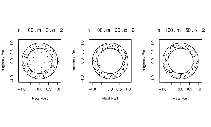
Figure 1: Scatter plots for product matrices: $n_{1}=n_{m+1}=n$, $n_{2}=\cdots=n_{m}=2n$, $\gamma_{n}=2m$

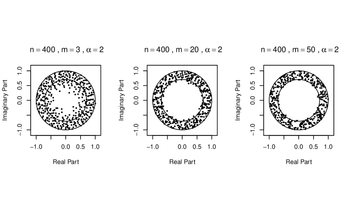
Figure 2: Scatter plots for product matrices: $n_{1}=n_{m+1}=n$, $n_{2}=\cdots=n_{m}=2n$, $\gamma_{n}=2m$

3 Proofs

The lemmas 3.1 and  3.2 below play a very important role in the proofs of our main results.

Lemma 3.1

(Theorem 1 in Jiang and Qi [18]). Let $\varphi(x)\geq 0$ be a measurable function defined on $[0,\infty).$ Assume the density of $(Z_{1},\cdots,Z_{n})\in\mathbb{C}^{n}$ is proportional to $\prod_{1\leq j<k\leq n}|z_{j}-z_{k}|^{2}\cdot\prod_{j=1}^{n}\varphi(|z_{j}|)$. Let $Y_{1},\cdots,Y_{n}$ be independent r.v.’s such that the density of $Y_{j}$ is proportional to $y^{2j-1}\varphi(y)I(y\geq 0)$ for every $1\leq j\leq n.$ Let $\mu_{n}$,$\nu_{n}$ and $\nu_{n}^{*}$ be defined as in (2.4) and (2.6), respectively. If $\{h_{n}\}$ are measurable functions such that $\nu_{n}\rightsquigarrow\nu$ for some probability measure $\nu$, then $\mu_{n}\rightsquigarrow\mu$ with $\mu=\mathrm{Unif}[0,2\pi]\otimes\nu$ . Taking $h_{n}(r)=r/a_{n}$, the conclusion still holds if “$(\mu_{n},\nu_{n},\mu,\nu)$” is replaced by “$(\mu_{n}^{*},\nu_{n}^{*},\mu^{*},\nu^{*})$” where $\mu^{*}$ is the distribution of $Re^{i\Theta}$ with $(\Theta,R)$ having the law of $\mathrm{Unif}[0,2\pi]\otimes\nu^{*}$.

Let $Y_{1},\cdots,Y_{n}$ be the independent random variables determined in Lemma 3.1 under model (2.1). Let $\{s_{j,r},~{}1\leq j\leq n,~{}1\leq r\leq m_{n}\}$ be independent random variables and $s_{j,r}$ follow a Gamma($l_{r}+j$) with density function $y^{l_{r}+j-1}e^{-y}I_{y>0}/\Gamma\left(l_{r}+j\right)$. Set

$$T_{j}=\prod_{r=1}^{m_{n}}s_{j,r},~{}~{}1\leq j\leq n.$$ (3.1)

Lemma 3.2

(Lemma 4 in Jiang and Qi [18]) Suppose $\{h_{n}(x);\,n\geq 1\}$ are measurable functions defined on $[0,\infty)$ and $\nu_{n}$’s are defined as in (2.4). Let $Y_{1},\cdots,Y_{n}$ be as in Lemma 3.1 and $\nu$ be a probability measure on $\mathbb{R}.$ Then $\nu_{n}\rightsquigarrow\nu$ if and only if

$$\lim_{n\to\infty}\frac{1}{n}\sum^{n}_{j=1}\mathbb{P}(h_{n}(Y_{j})\leq r)=H(r)$$

for every continuity point $r$ of $H(r)$, where $H(r):=\nu((-\infty,r]),\,r\in\mathbb{R}$.

The results in the following lemma are summarized from Lemmas 2.2 and 2.3 from Zeng [37].

Lemma 3.3

(Zeng [37]) We have

$$\mathbb{P}(T_{1}\leq x)\geq\mathbb{P}(T_{2}\leq x)\geq\cdots\geq\mathbb{P}(T_{n}\leq x)$$ (3.2)

for any $x\in[0,\infty)$, $(Y_{1}^{2},\cdots,Y_{n}^{2})\overset{d}{=}(T_{1},\cdots,T_{n})$, and

$$g(T_{1},\cdots,T_{n})\overset{d}{=}g(|z_{1}|^{2},\cdots,|z_{n}|^{2})$$ (3.3)

for any symmetric function $g(t_{1},\cdots,t_{n})$, where $\overset{d}{=}$ denotes equality in distribution.

Before we prove Theorem 2.4, we need to introduce more notation and preliminary results.

Define

$$\lambda_{k}(n)=\sum^{m_{n}}_{j=1}(\frac{n}{n_{j}})^{k},~{}~{}~{}k\geq 1$$ (3.4)

and

$$\theta_{k}(n)=\frac{\lambda_{k}(n)}{\lambda_{1}(n)},~{}~{}k\geq 1.$$ (3.5)

Note that $\lambda_{k}(n)\geq 1$ since $n_{1}=n$. Since $n\leq n_{j}$ for all $1\leq j\leq m_{n}$ we have $\lambda_{k}(n)$ is non-increasing in $k\geq 1$ for each $n$. Thus, we have $\theta_{k}(n)$ is non-increasing in $k\geq 1$, implying that $0<\theta_{k}(n)\leq\theta_{1}(n)=1$ for $k\geq 1$ and $n$.

We define a sequence of new distribution functions as follows

$$G_{n}(x)=\Big{(}\prod_{j=1}^{m_{n}}(1-\frac{n}{n_{j}}(1-x))\Big{)}^{1/\lambda_{1}(n)},~{}~{}~{}~{}x\in[0,1]$$ (3.6)

These distributions are obtained by letting $\gamma_{n}=\lambda_{1}(n)$ in equation (2.8). We have

$$F_{n}(x)=G_{n}^{\lambda_{1}(n)/\gamma_{n}}(x),~{}~{}~{}x\in[0,1].$$ (3.7)

Set $g_{n}(x)=\ln(G_{n}(x))$, $x\in(0,1]$. Then $g_{n}(x)\leq 0$ for $x\in(0,1]$. Using Taylor’s expansion $\ln(1-t)=-\sum^{\infty}_{k=1}\frac{t^{k}}{k}$, $|t|<1$, we have for $x\in(0,1]$

$$g_{n}(x)=-\sum_{k=1}^{\infty}\frac{\theta_{k}{(n)}}{k}(1-x)^{k}.$$ (3.8)

Note that $\theta_{1}(n)=1$ and $0<\theta_{k}(n)\leq 1$. We have the following inequalities

$$1-x\leq-g_{n}(x)\leq\sum_{k=1}^{\infty}\frac{1}{k}(1-x)^{k}=-\ln(x),~{}~{}~{}x\in(0,1].$$ (3.9)

The probability distribution $G_{n}$ over $[0,1]$ is defined via (3.6), and the same expression can not be extended beyond the interval $[0,1]$. The function $g_{n}(x)$, as the logarithm of $G_{n}$, has expansion (3.8) over $(0,1]$ only. However, $g_{n}$ can be extended to a region in the complex plane via the expression on the right-hand side of (3.8). Now we fix $0<\delta<1$. For any complex number $z$ such that $|z-1|\leq\delta$, we have from (3.9) that

$$\sum_{k=1}^{\infty}\left|-\frac{\theta_{k}{(n)}}{k}(1-z)^{k}\right|\leq\sum_{k=1}^{\infty}\frac{\theta_{k}{(n)}}{k}\delta^{k}=|g_{n}(1-\delta)|\leq\ln(\frac{1}{1-\delta}).$$ (3.10)

Therefore, we can extent $g_{n}(x)$ to be a complex analytic function on disk $D=\{z\in\mathbb{C}:|z-1|<1\}$, namely

$$g_{n}(z)=-\sum_{k=1}^{\infty}\frac{\theta_{k}{(n)}}{k}(1-z)^{k}.$$ (3.11)

Lemma 3.4

(Theorem 10.28 in Rudin [30]) Suppose $f_{j}$ is analytic on open set $\Omega\subset\mathbb{C}$ for $j=1,2,\cdots,$ and $f_{j}\rightarrow f$ uniformly on each compact subset of $\Omega$. Then $f$ is analytic on $\Omega$, and $f^{\prime}_{j}\rightarrow f^{\prime}$ uniformly on any compact subset on $\Omega$.

Lemma 3.5

Assume $\{n_{s}\}$ is a subsequence of $\{n\}$ such that $\lim_{s\to\infty}\theta_{k}(n_{s})=a_{k}\in[0,1]$ for all $k\geq 2$. Set $a_{1}=1$. Then

$$\lim_{s\to\infty}G_{n_{s}}(x)=G(x),~{}~{}~{}x\in(0,1],$$ (3.12)

where $G$ is a distribution function given by

$$G(x)=\exp(-\sum^{\infty}_{k=1}\frac{a_{k}}{k}(1-x)^{k}),~{}~{}~{}x\in(0,1].$$ (3.13)

$0<G(x)<1$ is analytic and strictly increasing over $(0,1)$.

Proof. In the proof we will use index $n$ instead of $n_{s}$ for the sake of brevity.

For each $\delta\in(0,1)$, set $K_{\delta}:=\{z\in\mathbb{C}:|z-1|\leq\delta\}$. It follows form (3.10) that $g_{n}(z)$ is uniformly bounded on $K_{\delta}$.

Set $g(z)=-\sum_{k=1}^{\infty}\frac{a_{k}}{k}(1-z)^{k}$. The radius of convergence of $g(z)$ satisfies

$$R=\frac{1}{\limsup_{n\rightarrow\infty}\left(\frac{a_{k}}{k}\right)^{1/k}}\geq\frac{1}{\limsup_{n\rightarrow\infty}\left(\frac{1}{k}\right)^{1/k}}=1,$$

i.e. $g(z)$ is well defined on disk $D=\{z\in\mathbb{C}:|z-1|<1\}$. For each $\delta\in(0,1)$, we have

$$\sup_{z\in K_{\delta}}|g_{n}(z)-g(z)|\leq\sum_{k=1}^{N}\frac{|a_{k}{(n)}-a_{k}|}{k}\delta^{k}+\sum_{k=N+1}^{\infty}\frac{\delta^{k}}{k}\leq\sum_{k=1}^{N}|a_{k}{(n)}-a_{k}|+\frac{\delta^{N+1}}{1-\delta},$$

which implies

$$\limsup_{n\rightarrow\infty}\sup_{z\in K_{\delta}}|g_{n}(z)-g(z)| \leq \limsup_{N\rightarrow\infty}\limsup_{n\rightarrow\infty}\Big{(}\sum_{k=1}^{N}|a_{k}{(n)}-a_{k}|+\frac{\delta^{N+1}}{1-\delta}\Big{)}$$

$$\leq \limsup_{N\rightarrow\infty}\frac{\delta^{N+1}}{1-\delta}$$

$$= 0,$$

that is, $g_{n}(z)$ converges to $g(z)$ uniformly on $K_{\delta}$.

Since $G_{n}(x)=\exp(g_{n}(x))$ for $x\in(0,1]$, we have (3.12) with $G(x)=\exp(g(x))$ for $x\in(0,1]$. Note that $g(x)$ is analytic, $g(x)<0$ and is strictly increasing for $x\in(0,1)$, we have $0<G(x)<1$ is analytic and strictly increasing over $(0,1)$. $\blacksquare$

Lemma 3.6

Assume $\{n_{s}\}$ is a subsequence of $\{n\}$ such that $G_{n_{s}}$ converges weakly to a distribution $G$, then $\lim_{s\to\infty}\theta_{k}(n_{s})=:a_{k}\in[0,1]$ for all $k\geq 2$, and $G$ has a representation (3.13).

Proof. Note that $0\leq\theta_{k}(n)\leq\theta_{1}(n)=1$ for all $n\geq 1$ and $k\geq 2$. By the diagonal argument, for every subsequence of $\{n\}$, we can find its further subsequence along which $\theta_{k}(n)$ has a subsequential limit in $[0,1]$ for all $k\geq 2$.

We aim to show that $\lim_{s\to\infty}\theta_{k}(n_{s})$ exists for all $k\geq 2$. If the conclusion is not true, then for some $k\geq 2$, say $k_{0}$, such that the limit of $\theta_{k_{0}}(n_{s})$ doesn’t exist. Then there exist two subsequences of $\{n_{s}\}$, say $\{n_{s^{\prime}}\}$ and $\{n_{s^{\prime\prime}}\}$, such that

$$\lim_{s^{\prime}\to\infty}\theta_{k_{0}}(n_{s^{\prime}})=a\neq b=\lim_{s^{\prime\prime}\to\infty}\theta_{k_{0}}(n_{s^{\prime\prime}}).$$ (3.14)

By the diagonal argument, we can find a further subsequence of $\{n_{s^{\prime}}\}$, along which $\theta_{k}(n_{s^{\prime}})$ has a subsequential limit $a_{k}\in[0,1]$ for each $k\geq 2$ with $a_{k_{0}}=a$. By Lemma 3.5 we have

$$G(x)=\exp(-\sum^{\infty}_{k=1}\frac{a_{k}}{k}(1-x)^{k}),~{}~{}~{}x\in(0,1].$$ (3.15)

since any subsequential limit of $G_{n_{s}}(x)$ is equal to $G(x)$ in $x\in(0,1]$. Similarly, we can find a further subsequence of $\{n_{s^{\prime\prime}}\}$, along which $\theta_{k}(n_{s^{\prime\prime}})$ has a subsequential limit $b_{k}\in[0,1]$ for each $\geq k$ with $b_{k_{0}}=b$. Again, using Lemma 3.5 we have

$$G(x)=\exp(-\sum^{\infty}_{k=1}\frac{b_{k}}{k}(1-x)^{k}),~{}~{}~{}x\in(0,1].$$ (3.16)

By combining (3.15) and (3.16), we have

$$\sum^{\infty}_{k=1}\frac{a_{k}}{k}(1-x)^{k}=\sum^{\infty}_{k=1}\frac{b_{k}}{k}(1-x)^{k},~{}~{}~{}x\in(0,1].$$

Therefore, we $a_{k}=b_{k}$ for all $k\geq 2$, which contradicts $a_{k_{0}}=a\neq b=b_{k_{0}}$ from (3.14). This proves the lemma. $\blacksquare$

Proof of Theorem 2.4. First, we assume $F_{n}$ converges weakly to a distribution function $F$. We will show $F$ must be of one of the three types given in Theorem 2.4.

Review the definitions of $\lambda_{k}(n)$ and $\theta_{k}(n)$ in (3.4) and (3.5), respectively.

We consider the sequence $\lambda_{1}(n)/\gamma_{n}$. At this moment, we don’t know yet whether $r_{n}:=\lambda_{1}(n)/\gamma_{n}$ has a limit. We assume that $\{n_{s}\}$ is any subsequence of $\{n\}$ such that

$$\lim_{s\to\infty}r_{n_{s}}=\lim_{s\to\infty}\frac{\lambda_{1}(n_{s})}{\gamma_{n_{s}}}=c_{1}\in[0,\infty].$$ (3.17)

We consider the following three cases individually: $c_{1}\in(0,1)$, $c_{1}=\infty$, and $c_{1}=0$. From (3.7) we have that

$$G_{n}(x)=F_{n}^{1/r_{n}}(x)~{}~{}~{}~{}~{}x\in(0,1].$$ (3.18)

Case 1. $c_{1}\in(0,\infty)$ in (3.17).

In this case, we see that $G_{n_{s}}$ converges weakly to $G(x)=F^{1/c_{1}}(x)$. By applying Lemma 3.6, we have $\lim_{s\to\infty}\theta_{k}(n_{s})=:a_{k}\in[0,1]$ for all $k\geq 2$, and $G$ has a representation (3.13), which implies $F$ has a representation (2.11) with $c_{k}=c_{1}a_{k}$ for $k\geq 2$. This shows that $F$ is of type I.

Case 2. $c_{1}=0$ in (3.17).

In view of (3.7), (3.8) and (3.9), we have for any $x\in(0,1)$

$$1\geq F_{n_{s}}(x)=G_{n}^{r_{n_{s}}}(x)=\exp(r_{n_{s}}g_{n}(x))\geq\exp(r_{n_{s}}\ln(x))\to 1$$

as $s\to\infty$, which implies $F(x)=1$ for $x\in(0,1)$ and thus $F$ is of type II.

Case 3. $c_{1}=\infty$ in (3.17).

Using the same equations as in the proof for Case 2, we have for any $x\in(0,1)$

$$0\leq F_{n_{s}}(x)=G_{n}^{r_{n_{s}}}(x)=\exp(r_{n_{s}}g_{n}(x))\leq\exp(r_{n_{s}}(1-x))\to 0$$

as $s\to\infty$, which implies $F(x)=0$ for $x\in(0,1)$ and thus $F$ is of type III.

We have proved that there are only three types of limiting distributions for $F_{n}$. Next, we will show the necessary and sufficient conditions in parts (a), (b), and (c).

Sufficiency for parts (b) and (c) has been proved. In fact, for part (b), condition (2.12) must be true when $F$ is of Type II, otherwise, there exists a subsequential limit $c_{1}$ of $r_{n}$ with $c_{1}\in(0,\infty)$ or $c_{1}=\infty$, such that $F$ is of Type I or Type III, respectively, yielding a contradiction. A similar argument can be used to show (2.13) in part (c).

Finally, we need to prove part (a). The sufficiency has been proved in Case 1 above. Assume $F_{n}$ converges weakly to $F$, which is of Type I. We show (2.10), or equivalently, we show the following statements

Statement 1: $r_{n}=\lambda_{1}(n)/\gamma_{n}$ has a limit $c_{1}\in(0,\infty)$;

Statement 2: For any $k\geq 2$, $\theta_{k}(n)$ has a finite limit.

If Statement 1 is not true, then there are subsequences of $\{n\}$, say, $\{n_{s}\}$ and $\{n_{s^{\prime}}\}$ such that

$$\lim_{s\to\infty}r_{s}=a\neq b=\lim_{s^{\prime}\to\infty}r_{s^{\prime}},$$

and $a,b\in(0,\infty)$. Any subsequential limit of $r_{n}$ must be a finite positive number since $F$ is of Type I.

From (3.18), we have $G_{n_{s}}$ converges weakly to $F^{1/a}$ and $G_{n_{s^{\prime}}}$ converges weakly to $F^{1/b}$. Then it follows from Lemma 3.6 that

$$F^{1/a}(x)=\exp(-\sum^{\infty}_{k=1}\frac{a_{k}}{k}(1-x)^{k}),~{}~{}~{}x\in(0,1]$$

and

$$F^{1/b}(x)=\exp(-\sum^{\infty}_{k=1}\frac{b_{k}}{k}(1-x)^{k}),~{}~{}~{}x\in(0,1]$$

where $a_{1}=b_{1}=1$ and $a_{k},b_{k}\in[0,1]$ for all $k\geq 2$. We conclude that

$$a\sum^{\infty}_{k=1}\frac{a_{k}}{k}(1-x)^{k}=b\sum^{\infty}_{k=1}\frac{b_{k}}{k}(1-x)^{k},~{}~{}~{}x\in(0,1].$$

Since the functions on both sides of the above equation are analytic, their first derivatives at $x=1$ must be the same, which leads to $a=b$, contradictory to the assumption $a\neq b$. Therefore, Statement 1 is true, that is, $r_{n}$ has a limit in $(0,\infty)$.

Given $\lim_{n\to\infty}r_{n}=c_{1}$, from (3.18) we have $G_{n}$ converges weakly to $F^{1/c_{1}}$. Again, by using Lemma 3.6, we have $a_{k}:=\lim_{n\to\infty}\theta_{k}(n)$ exists for all $k\geq 2$ and $a_{k}\in[0,1]$. This proves Statement 2. The proof of the theorem is completed. $\blacksquare$

The following result is an extension of Lemma 2.3 in Zeng  [37]. We allow $m_{n}$ to change with $n$.

Lemma 3.7

Assume $\{m_{n}\}$ is a sequence of positive integers. Then

$$\frac{1}{\lambda_{1}(n)}\ln\frac{T_{[\mathrm{nx}]}}{\prod_{r=1}^{m_{n}}(l_{r}+n)}-\ln G_{n}(x)\stackrel{{\scriptstyle p}}{{\rightarrow}}0,~{}~{}x\in(0,1],$$ (3.19)

where $[nx]$ denotes the integer part of $nx$, $T_{j}$ is defined in (3.1), $\lambda_{1}(n)$ is defined in (3.4), and $G_{n}$ is defined in (3.6).

Proof. We have $\ln T_{j}=\sum_{r=1}^{m}\ln s_{j,r}$ for $j\geq 1$. Since $s_{j,r}$ has a Gamma($l_{r}+j$) distribution, we have

$$\mu_{j,r}=\mathbb{E}\left(s_{j,r}\right)=l_{r}+j,~{}~{}{\mathrm{Var}}\left(s_{j,r}\right)=l_{r}+j$$

and the moment generating function of $\ln s_{j,r}$ is

$$m_{j}(t)=\mathbb{E}\big{(}e^{t\ln s_{j,r}}\big{)}=\frac{\Gamma\left(l_{r}+j+t\right)}{\Gamma\big{(}l_{r}+j\big{)}},~{}~{}~{}t>-(l_{r}+j).$$

It follows that

$$\mathbb{E}\big{(}\ln s_{j,r}\big{)}=\frac{d}{dt}m_{j}(t)\Big{|}_{t=0}=\frac{\Gamma^{\prime}\left(l_{r}+j\right)}{\Gamma\left(l_{r}+j\right)}=\psi\left(l_{r}+j\right),$$

where $\psi(x)=\Gamma^{\prime}(x)/\Gamma(x)$ is a digamma function. Thus, we have

$$\mathbb{E}\big{(}\ln T_{j}\big{)}=\sum_{r=1}^{m_{n}}\mathbb{E}\left(\ln s_{j,r}\right)=\sum_{r=1}^{m_{n}}\psi\left(l_{r}+j\right).$$ (3.20)

Set $\eta(t)=t-1-\ln t$ for $t>0$. Then $\eta(t)\geq 0$ for $t>0$.

Trivially, we have for any $1\leq j\leq n$

$$\ln\frac{T_{j}}{\prod_{r=1}^{m_{n}}\mu_{j,r}}-\sum_{r=1}^{m_{n}}\ln(\frac{l_{r}+j}{l_{r}+n})=\sum_{r=1}^{m_{n}}(\frac{s_{j,r}}{\mu_{j,r}}-1)-\sum_{r=1}^{m_{n}}\eta(\frac{s_{j,r}}{\mu_{j,r}}).$$ (3.21)

It can be seen that for $1\leq j\leq n$

$${\mathrm{Var}}\left(\sum_{r=1}^{m_{n}}\Big{(}\frac{s_{j,r}}{\mu_{j,r}}-1\Big{)}\right)=\sum_{r=1}^{m_{n}}\frac{{\mathrm{Var}}\left(s_{j,r}\right)}{\mu_{j,r}^{2}}=\sum_{r=1}^{m_{n}}\frac{1}{l_{r}+j}\leq\sum_{r=1}^{m_{n}}\frac{n}{j(l_{r}+n)}=\frac{\lambda_{1}(n)}{j}.$$

Fix $x\in(0,1]$. Set $j=j_{n}=[nx]$. Then

$$\mathrm{Var}\Big{(}\frac{1}{\lambda_{1}(n)}\sum_{r=1}^{m_{n}}(\frac{s_{j_{n},r}}{\mu_{j_{n},r}}-1)\Big{)}\leq\frac{1}{\lambda_{1}(n)j_{n}}\leq\frac{1}{j_{n}}\to 0$$

as $n\to\infty$. By Chebyshev inequality, we obtain

$$\frac{1}{\lambda_{1}(n)}\sum_{r=1}^{m_{n}}(\frac{s_{j_{n},r}}{\mu_{j_{n},r}}-1)\stackrel{{\scriptstyle p}}{{\rightarrow}}0.$$ (3.22)

From (3.21) and (3.20) we have

$$\mathbb{E}\Big{(}\sum_{r=1}^{m_{n}}\eta\big{(}\frac{s_{j,r}}{\mu_{j,r}}\big{)}\Big{)}=\sum_{r=1}^{m_{n}}\ln\mu_{j,r}-\mathbb{E}\sum_{r=1}^{m_{n}}\ln s_{j,r}=-\sum_{r=1}^{m_{n}}\big{(}\psi(l_{r}+j)-\ln(l_{r}+j)\big{)}.$$

We need the following approximation for $\psi$

$$\psi(t)-\ln t=-\frac{1}{2t}+O\Big{(}\frac{1}{t^{2}}\Big{)}\mbox{ as }t\to\infty;$$

See, e.g., Formula 6.3.18 in Abramowitz and Stegun [1]. With $j_{n}=[nx]$, we have

$$\frac{1}{\lambda_{1}(n)}\mathbb{E}\Big{(}\sum_{r=1}^{m_{n}}\eta\big{(}\frac{s_{j,r}}{\mu_{j,r}}\big{)}\Big{)}=\frac{O(1)}{\lambda_{1}(n)}\sum_{r=1}^{m_{n}}\frac{1}{l_{r}+j_{n}}\leq\frac{O(1)}{\lambda_{1}(n)}\frac{\lambda_{1}(n)}{j_{n}}=O(\frac{1}{j_{n}})\to 0$$

as $n\to\infty$, which implies

$$\frac{1}{\lambda_{1}(n)}\sum_{r=1}^{m_{n}}\eta\left(\frac{s_{j,r}}{\mu_{j,r}}\right)\stackrel{{\scriptstyle p}}{{\rightarrow}}0$$ (3.23)

by Chebyshev inequality since $\sum_{r=1}^{m}\eta\left(\frac{s_{j,r}}{\mu_{j,r}}\right)\geq 0$. Therefore, combining (3.21), (3.22) and (3.23), we obtain

$$\frac{1}{\lambda_{1}(n)}\ln\frac{T_{[\mathrm{nx}]}}{\prod_{r=1}^{m_{n}}(l_{r}+[nx])}-\ln G_{n}(\frac{[nx]}{n})\stackrel{{\scriptstyle p}}{{\rightarrow}}0,~{}~{}~{}x\in(0,1].$$ (3.24)

From (3.8), we have $0<g_{n}^{\prime}(t)=\sum^{\infty}_{r=1}\theta_{k}(n)(1-t)^{k-1}\leq\frac{1}{t}$ for $0<t\leq 1$, and hence,

$$|\ln G_{n}(\frac{[nx]}{n})-\ln G_{n}(x)|=|g_{n}(\frac{[nx]}{n})-g_{n}(x)|\leq\sup_{\frac{[nx]}{n}\leq t\leq x}g^{\prime}_{n}(t)|\frac{[nx]}{n}-x|\leq\frac{1}{[nx]}\to 0$$

as $n\to\infty$. This, coupled with (3.24), yields (3.19). $\blacksquare$

Proof of Theorem 2.3. Assume $F_{n}$ converges weakly to a distribution $F$. The conclusion in the theorem follows from Lemma 3.1 and Lemma 3.2 if we can prove

$$\lim_{n\to\infty}\frac{1}{n}\sum^{n}_{j=1}\mathbb{P}(h_{n}(Y_{j})\leq y)=F^{*}(y)$$

for every continuity point $y$ of $F^{*}$. According to (3.3), it is equivalent to show

$$\lim_{n\to\infty}\frac{1}{n}\sum^{n}_{j=1}\mathbb{P}\Big{(}\frac{1}{a_{n}}T_{j}^{1/\gamma_{n}}\leq y\Big{)}=F^{*}(y)$$ (3.25)

for every continuity point $y$ of $F^{*}$. Since $a_{n}=\prod^{m_{n}}_{r=1}n_{r}^{1/\gamma_{n}}=\prod^{m_{n}}_{r=1}(l_{r}+n)^{1/\gamma_{n}}$, we have

$$\mathbb{P}\Big{(}\frac{1}{a_{n}}T_{j}^{1/\gamma_{n}}\leq y\Big{)}=\mathbb{P}\Big{(}\frac{1}{\gamma_{n}}\ln\frac{T_{j}}{\prod_{r=1}^{m_{n}}\left(l_{r}+j\right)}\leq\ln y\Big{)},~{}~{}~{}y>0.$$ (3.26)

We also have the following two inequalities

$$\frac{j}{n}\mathbb{P}\Big{(}\frac{1}{a_{n}}T_{j}^{1/\gamma_{n}}\leq y\Big{)}\leq\frac{1}{n}\sum_{j=1}^{n}\mathbb{P}\Big{(}\frac{1}{a_{n}}T_{j}^{1/\gamma_{n}}\leq y\Big{)}\leq\frac{j}{n}+\mathbb{P}\Big{(}\frac{1}{a_{n}}T_{j}^{1/\gamma_{n}}\leq y\Big{)},$$ (3.27)

which follow from the monotonicity in (3.2) directly.

Case 1. Assume $F$ is of Type I.

In this case, $F$ is strictly increasing in $[0,1]$ with $F(x)>0$ for any $x\in(0,1]$ and $\lim_{n\to\infty}F_{n}(x)=F(x)$, and $F^{*}$ is given by (2.14). We note that $\lambda_{1}(n)/\gamma_{n}$ converges to a non-zero constant from Theorem 2.4. From (3.19), we have for any $x\in(0,1]$

$$\frac{1}{\gamma_{n}}\ln\frac{T_{[\mathrm{nx}]}}{\prod_{r=1}^{m_{n}}(l_{r}+n)}-\ln F_{n}(x)=\frac{\lambda_{1}(n)}{\gamma_{n}}\Big{(}\frac{1}{\lambda_{1}(n)}\ln\frac{T_{[\mathrm{nx}]}}{\prod_{r=1}^{m_{n}}(l_{r}+n)}-\ln G_{n}(x))\Big{)}\stackrel{{\scriptstyle p}}{{\rightarrow}}0,$$

yielding

$$\frac{1}{\gamma_{n}}\ln\frac{T_{[\mathrm{nx}]}}{\prod_{r=1}^{m_{n}}(l_{r}+n)}-\ln F(x)\stackrel{{\scriptstyle p}}{{\rightarrow}}0.$$ (3.28)

From (3.26) we get

$$\mathbb{P}\Big{(}\frac{1}{a_{n}}T_{j}^{1/\gamma_{n}}\leq y\Big{)}=\mathbb{P}\Big{(}\frac{1}{\gamma_{n}}\ln\frac{T_{j}}{\prod_{r=1}^{m_{n}}\left(l_{r}+j\right)}-\ln F(x)\leq\ln\frac{y}{F(x)}\Big{)}$$ (3.29)

for $y>0$ and any $x$ with $F(x)>0$.

Now we are ready to show (3.25) when $F(0)<y<1$, $y\leq F(0)$, and $y\geq 1$.

We first assume $F(0)<y<1$. Let $\delta\in(0,1)$ be any given number such that

$$F(0)<y-\delta<y<y+\delta<1.$$

Then $0<F^{*}(y-\delta)<F^{*}(y)<F^{*}(y+\delta)<1$.

By setting $x=F^{*}(y+\delta)$, $j=[nx]$ in (3.27) and (3.29) and using (3.28), we have

$$\limsup_{n\rightarrow\infty}\frac{1}{n}\sum_{j=1}^{n}\mathbb{P}\Big{(}\frac{1}{a_{n}}T_{j}^{1/\gamma_{n}}\leq y\Big{)}$$

$$\leq \limsup_{n\rightarrow\infty}\frac{[nx]}{n}+\limsup_{n\rightarrow\infty}\mathbb{P}\Big{(}\frac{1}{\gamma_{n}}\ln\frac{T_{[nx]}}{\prod_{r=1}^{m_{n}}\Big{(}l_{r}+[nx]\Big{)}}-\ln F(x)\leq\ln\frac{y}{y+\delta}<0\Big{)}$$

$$= x=F^{*}(y+\delta).$$

By setting $x=F^{*}(y-\delta)$ and $j=[nx]$ in (3.27) and (3.29), and using (3.28) again, we have

$$\liminf_{n\rightarrow\infty}\frac{1}{n}\sum_{j=1}^{n}\mathbb{P}\Big{(}\frac{1}{a_{n}}T_{j}^{1/\gamma_{n}}\leq y\big{)} \geq \liminf_{n\rightarrow\infty}\frac{[nx]}{n}\mathbb{P}\Big{(}\frac{1}{\gamma_{n}}\ln\frac{T_{[nx]}}{\prod_{r=1}^{m_{n}}\left(l_{r}+[nx]\right)}-\ln F(x)\leq\ln\frac{y}{y-\delta}\Big{)}$$

$$= x=F^{*}(y-\delta).$$

Since $F^{*}(y)$ is continuous, we obtain (3.25) by letting $\delta$ tend to $0$.

Assume $y\leq F(0)$. For any $y_{1}\in(F(0),1)$, we have

$$\limsup_{n\to\infty}\frac{1}{n}\sum_{j=1}^{n}\mathbb{P}\Big{(}\frac{1}{a_{n}}T_{j}^{1/\gamma_{n}}\leqslant y\Big{)}\leq\lim_{n\to\infty}\frac{1}{n}\sum_{j=1}^{n}\mathbb{P}\Big{(}\frac{1}{a_{n}}T_{j}^{1/\gamma_{n}}\leqslant y_{1}\Big{)}=F^{*}(y_{1}),$$

which tends to $F^{*}(F(0))=0$ by letting $y_{1}\downarrow F(0)$ since $F^{*}(y)$ is continuous. Similarly, when $y\geq 1$ we have for any $y_{2}\in(F(0),1)$

$$\liminf_{n\to\infty}\frac{1}{n}\sum_{j=1}^{n}\mathbb{P}\Big{(}\frac{1}{a_{n}}T_{j}^{1/\gamma_{n}}\leqslant y\Big{)}\geq\lim_{n\to\infty}\frac{1}{n}\sum_{j=1}^{n}\mathbb{P}\Big{(}\frac{1}{a_{n}}T_{j}^{1/\gamma_{n}}\leqslant y_{2}\Big{)}=F^{*}(y_{2}),$$

which tends to $F^{*}(F(1))=1$ by letting $y_{2}\uparrow 1$. In both cases, (3.25) still holds.

Case 2. Assume $F$ is of Type II.

From Theorem 2.4, we have $\lim_{n\to\infty}\lambda_{1}(n)/\gamma_{n}=0$. Since $\ln G_{n}(x)=g_{n}(x)$ is bounded for any fixed $x\in(0,1)$, we have from (3.19) that

$$\frac{1}{\gamma_{n}}\ln\frac{T_{[\mathrm{nx}]}}{\prod_{r=1}^{m_{n}}(l_{r}+n)}\overset{p}{\to}0$$ (3.30)

for any $x\in(0,1]$.

Review $F^{*}$ in (2.15).

When $y\leq 0$, (3.25) is trivially true.

When $y\in(0,1)$, we have $\ln y<0$. For any $x\in(0,1)$, set $j=[nx]$. Then from (3.27), (3.26) and (3.30) we have

$$\limsup_{n\rightarrow\infty}\frac{1}{n}\sum_{j=1}^{n}\mathbb{P}\Big{(}\frac{1}{a_{n}}T_{j}^{1/\gamma_{n}}\leq y\Big{)}\leq\limsup_{n\rightarrow\infty}\frac{[nx]}{n}+\limsup_{n\rightarrow\infty}\mathbb{P}\Big{(}\frac{1}{\gamma_{n}}\ln\frac{T_{[nx]}}{\prod_{r=1}^{m_{n}}\Big{(}l_{r}+[nx]\Big{)}}\leq\ln y\Big{)}=x.$$

Since $x$ can be arbitrarily small, we have

$$\lim_{n\rightarrow\infty}\frac{1}{n}\sum_{j=1}^{n}\mathbb{P}\Big{(}\frac{1}{a_{n}}T_{j}^{1/\gamma_{n}}\leq y\Big{)}=0=F^{*}(y).$$

That is, (3.25) is true.

When $y>1$, $\ln y>0$. Again, for any $x\in(0,1)$, setting $j=[nx]$ and using (3.27), (3.26) and (3.30), we have

$$\liminf_{n\to\infty}\frac{1}{n}\sum_{j=1}^{n}\mathbb{P}\Big{(}\frac{1}{a_{n}}T_{j}^{1/\gamma_{n}}\leqslant y\Big{)}\geq x.$$

By letting $x\uparrow 1$ we have

$$\lim_{n\to\infty}\frac{1}{n}\sum_{j=1}^{n}\mathbb{P}\Big{(}\frac{1}{a_{n}}T_{j}^{1/\gamma_{n}}\leqslant y\Big{)}=1=F^{*}(y).$$

This completes the proof of (3.25).

Case 3. Assume $F$ is of Type III.

This time, we have $\lim_{n\to\infty}\lambda_{1}(n)/\gamma_{n}=\infty$.

$$\frac{1}{\gamma_{n}}\ln\frac{T_{[\mathrm{nx}]}}{\prod_{r=1}^{m_{n}}(l_{r}+n)}\overset{p}{\to}-\infty$$

for any $x\in(0,1)$. We can prove (3.25) by using similar lines to Case 2. We omit the details.

The proof of Theorem 2.3 is completed. $\blacksquare$

Proof of Theorem 2.1. From Theorems 2.3 and  2.4, we have $\mu_{n}\rightsquigarrow\mathrm{Unif}[0,2\pi)\otimes\nu$ as $n\to\infty$, where $\nu$ has a a density function $f^{*}(r)=\frac{d}{dr}F^{*}(r)=\frac{1}{f(F^{*}(r))}$, $r\in[F(0),1]$. Let $\Theta$ $R$ are two independent random variables, $\Theta$ is uniformly distributed over $[0,2\pi)$ and $R$ has density function $f^{*}$. Consider the transformation $Z=R\exp(i\Theta)=R\cos(\Theta)+iR\sin(\Theta)=(R\cos(\Theta),R\sin(\Theta))=:(X,Y)$. Note that the Jacobian for transformation $(x,y)=(r\cos(\theta),r\sin(\theta))$ is $r=\sqrt{x^{2}+y^{2}}=|z|$, where $z=re^{i\theta}=x+iy$. The joint density function of $Z=(X,Y)$ is given by $\frac{1}{2\pi}\frac{f^{*}(|z|)}{|z|}=\frac{1}{2\pi f(F^{*}|z|)|z|}I(F(0)\leq|z|\leq 1)$. Since $\hat{\mu}_{n}$ is obtained under transformation $(x,y)=(r\cos(\theta),r\sin(\theta))$, by the continuous mapping theorem, we $\hat{\mu}_{n}$ converges with probability one to $Z=(X,Y)$ which has a joint density $\frac{1}{2\pi f(F^{*}|z|)|z|}I(F(0)\leq|z|\leq 1)$. $\blacksquare$

Proof of Theorem 2.2. Using the same notations as in the proof for Theorem 2.1, we have $P(R=1)=1$. Therefore, we can easily conclude that $Z$ has a uniform distribution on the unit circle. $\blacksquare$

Acknowledgements. The authors would like to thank an anonymous referee for his/her careful reading of the manuscript and suggestion which has improved the layout of the manuscript. The research of Yongcheng Qi was supported in part by NSF Grant DMS-1916014.

References

[1]
Abramowitz, M. and Stegun, I. A. (1972). Handbook of Mathematical
Functions. Dover, New York.
[2]
Adhikari, K., Reddy, N. K., Reddy, T. R. and Saha, K. (2016).
Determinantal point processes in the plane from products of random
matrices. Ann. Inst. H. Poincare Probab. Statist. 52 (1),
16-46.
[3]
Akemann, G., Baik, J. and Francesco, P. D. (2011). The Oxford
Handbook of Random Matrix Theory. Oxford University Press, New
York.
[4]
Bai, Z.D. (1997). Circular law. Annals of Probability 25,
494-529
[5]
Beenakker, C. W. J. (1997). Random-matrix theory of quantum
transport. Rev. Mod. Phys. 69, 731-809.
[6]
Bordenave, C. (2011). On the spectrum of sum and product of
non-Hermitian random matrices. Elect. Comm. in Probab. 16,
104-113.
[7]
Chang, S., Li, D. and Qi, Y. (2018). Limiting distributions of
spectral radii for product of matrices from the spherical ensemble.
Journal of Mathematical Analysis and Applications 461, 1165-1176.
[8]
Chang, S. and Qi, Y. (2017). Empirical distribution of scaled
eigenvalues for product of matrices from the spherical ensemble.
Statistics & Probability Letters 128, 8-13.
[9]
Couillet, R. and Debbah, M. (2011). Random matrix methods for
wireless communications. Cambridge Univ Press.
[10]
Ginibre, J. (1965). Statistical ensembles of complex, quaternion,
and real matrices. J. Math. Phys. 6, 440-449.
[11]
Girko, V.L. (1984). The circular law. Teoriya Veroyatnostei i
ee Primeneniya 29, 669-679.
[12]
Götze F., Kösters H. and Tikhomirov, A. (2015). Asymptotic
spectra of matrix-valued functions of independent random matrices
and free probability. Random Matrices: Theory Appl. 4,
1550005.
[13]
Götze, F. and Tikhomirov, T. (2010). On the asymptotic spectrum
of products of independent random matrices. http://arxiv.org/pdf/1012.2710v3.pdf.
[14]
Götze, F. and Tikhomirov, T. (2010). The circular law for random matrices. Annals of Probability 38, 1444-1491.
[15]
Ipsen, J. R. (2015). Products of Independent Gaussian Random
Matrices. Doctoral Dissertation. Bielefeld University.
[16]
Jiang, T. (2009). Approximation of Haar distributed matrices and
limiting distributions of eigenvalues of Jacobi ensembles. Probability Theory and Related Fields 144 (1), 221-246.
[17]
Jiang, T. and Qi, Y. (2017). Spectral radii of large non-Hermitian
random matrices. Journal of Theoretical Probability 30,
326-364.
[18]
Jiang, T. and Qi, Y. (2019). Empirical distributions of eigenvalues
of product ensembles. Journal of Theoretical Probability 32,
353-394,
[19]
Johnstone, I. (2001). On the distribution of the largest eigenvalue
in principal components analysis. Ann. Stat. 29, 295-327.
[20]
Johnstone, I. (2008). Multivariate analysis and Jacobi ensembles:
Largest eigenvalue, Tracy-Widom limits and rates of convergence.
Ann. Stat., 36 (6), 2638-2716.
[21]
Lambert, G. (2018). Limit theorem for biorthogonal ensembles and
related combinatorial identities. Adv. Math. 329, 590-648.
[22] Mezzadri, F. and Snaith, N. C. (2005). Recent perspectives in random matrix theory and number theory.
Cambridge Univ Press.
[23]
O’Rourke, S. and Soshnikov, A. (2011). Products of independent
non-Hermitian random matrices. Electrical Journal of
Probability 16(81), 2219-2245.
[24]
O’Rourke, S., Renfrew, D., Soshnikov, A. and Vu, V. (2015).
Products of independent elliptic random matrices. Journal of
Statistical Physics 160, 89-119.
[25]Pan, G. and Zhou, W. (2010).
Circular law, extreme singular values and potential theory. J. Multivariate Anal. 101,
645-656.
[26]
Qi, Y. and Xie, M. (2020). Spectral radii of products of random
rectangular matrices. Journal of Theoretical Probability 33,
2185-2212.
[27]
Rider, B. C. (2003). A limit theorem at the edge of a non-Hermitian
random matrix ensemble. J. Phys. A 36(12), 3401-3409.
[28]
Rider, B. C. (2004). Order statistics and Ginibre’s ensembles.
Journal of Statistical Physics 114, 1139-1148.
[29]
Rider, B. C. and Sinclair, C. D. (2014). Extremal laws for the real
Ginibre ensemble. Ann. Appl. Probab. 24(4), 1621-1651.
[30]
Rudin, W. (1986). Real and Complex Analysis. 3rd edn. McGraw-Hill,
New York.
[31] Tao, T. and Vu, V. (2010). Random matrices: universality of ESD and the circular law.
Annals of Probability 38, 2023-2065.
[32]
Tracy, C. A. and Widom, H. (1994). Level-spacing distributions and
Airy kernal. Comm. Math. Physics 159, 151-174.
[33]
Tracy, C. A. and Widom, H. (1996). On the orthogonal and symplectic
matrix ensembles. Comm. Math. Physics 177, 727-754.
[34]
Wigner, E. P. (1955). Characteristic vectors of bordered matrices
with infinite dimensions. Ann. Math. 62, 548-564.
[35]
Wishart, J. (1928). The generalized product moment distribution in
samples from a normal multivariate population. Biometrika 20,
35-52.
[36]
Zeng, X. (2016). Eigenvalues distribution for products of
independent spherical ensembles. J. Phys. A: Math. Theor. 49,
235201.
[37]
Zeng, X. (2017). Limiting empirical distribution for eigenvalues of
products of random rectangular matrices. Statistics and
Probability Letters 126, 33-40.