On the possible orbital motion of Sgr A* in the smooth potential of the Milky Way

Abstract

The modern accuracy of measurements allows the residual/peculiar (Galactocentric) velocity of the supermassive black hole (SMBH) in our Galaxy, Sgr A^∗, on the order of several kilometers per second. We integrate possible orbits of the SMBH along with the surrounding nuclear star cluster (NSC) for a barred model of the Galaxy using modern constraints on the components of the SMBH Galactocentric velocity. Is is shown that the range of oscillations of the SMBH + NSC in a regular Galactic field in the plane of the Galaxy allowed by these constraints strongly depends on the set of central components of the Galactic potential. If the central components are represented only by a bulge/bar, for a point estimate of the SMBH Galactocentric velocity, the oscillation amplitude does not exceed 7 pc in the case that a classical bulge is present and reaches 25 pc if there is no bulge; with SMBH velocity components within the $2\sigma$ significance level, the amplitude can reach 15 and 50 pc, respectively. However, when taking into account the nuclear stellar disk (NSD), even in the absence of a bulge, the oscillation amplitude is only 5 pc for the point estimate of the SMBH velocity, and 10 pc for the $2\sigma$ significance level. Thus, the possible oscillations of the SMBH + NSC complex from the confirmed components of the Galaxy’s potential are mostly limited by the NSD, and even taking into account the uncertainty of the mass of the latter, the oscillation amplitude can hardly exceed $13\,\text{pc}=6^{\prime}$.

1 Introduction

Modeling the orbital motions of S stars in the vicinity of the supermassive black hole (SMBH) Sgr A^∗  in the central region of the Milky Way allows accurate estimates of the distance $R(\text{BH})$ from the Sun to this object (see, e.g., Bland-Hawthorn & Gerhard 2016; de Grijs & Bono 2016). The most reliable are the results of recent analyses of data on the star S2 (S0-2): GRAVITY Collaboration et al. (2019) reported $R(\text{BH})=8178\pm 13_{\text{\,stat.}}\pm 22_{\text{\,sys.}}$ pc; Do et al. (2019) measured $R(\text{BH})=7946\pm 50\,(\text{stat.})\pm 32\,(\text{sys.})$ pc (both estimates assume General Relativity is true). It is commonly believed that the SMBH is exactly at the (bary)center of the Galaxy (e.g., de Grijs & Bono 2016). Then $R(\text{BH})$ measurements can be considered as estimates of the distance $R_{0}$ to the center of the Galaxy: $R_{0}=R(\text{BH})$. Moreover, such estimates are absolute (i.e., not using luminosity calibrations; see the classification in Nikiforov 2004) and have high (at least formal) precision and accuracy.

At the moment, the $R_{0}$ estimates obtained by the orbit method by the two research groups differ significantly (at the $3.6\sigma$ level for the above estimates, taking into account the systematic uncertainties specified by the authors). Yet $R(\text{BH})$ measurements already have high precision, which will grow in the future as data accumulate. It makes sense to consider the scale of the possible deviation of the SMBH from the barycenter of the Galaxy, which may not be negligible compared to the current and future accuracy of $R(\text{BH})$ estimates. Blitz (1994) pointed to the possibility of oscillations of the Sgr A^∗ system and other central Galactic mass concentrations in a “fairly shallow” bar potential. Some explorations of the dynamics of SMBHs in galactic cores show that the displacement of the SMBH from the geometric center of the galaxy due to interaction with globular clusters and stars can reach several parsecs (Kondrat’ev & Orlov 2008; Di Cintio et al. 2019). In the case of M87, the SMBH appears to be off-centered in the parent galaxy by $6.8\pm 0.8$ pc (Batcheldor et al. 2010).

The assumption that the SMBH is essentially at rest at the Galactic center is based largely on the marginally nonzero peculiar proper motion of Sgr A^∗ (e.g., Reid & Brunthaler 2004; Bland-Hawthorn & Gerhard 2016). However the accuracy of modern measurements does not exclude the residual velocity of Sgr A^∗ in Galactic longitude and the peculiar radial velocity of the SMBH on the order of several kilometers per second (see Sect. 2). Further in this paper, for a barred model of the Galaxy (Sect. 3), we determine possible orbits of the SMBH, along with its host nuclear star cluster (NSC), using modern constraints on the components of the SMBH residual/peculiar velocity to estimate the scale of possible SMBH + NSC oscillations relative to the barycenter (Sect. 4) and then we discuss the results (Sect. 5).

2 Measurements of the peculiar/residual velocity of the SMBH (Sgr A*)

In this work, we consider the SMBH and the NSC as a single complex with a common orbit in a regular Galactic field. Indeed, the significant mass ${\sim}2\times 10^{7}M_{\odot}$ and compactness (the effective radius is ${\sim}5$ pc) of the NSC (e.g., Bland-Hawthorn & Gerhard 2016; Gallego-Cano et al. 2020) should greatly limit the possible deviations of the black hole from its center (we test this in Sect. 5). The detection of a stellar cusp around the SMBH (e.g., Gallego-Cano et al. 2020) indicates a partial relaxation of the NSC (e.g., Baumgardt et al. 2018). In the projection, the SMBH is observed near the center of the NSC (e.g., Feldmeier et al. 2014; Gallego-Cano et al. 2020). Therefore, considering the SMBH and NSC as a single complex in which the SMBH is located near its barycenter seems acceptable, at least in the first approximation. The SMBH + NSC complex itself can undergo oscillations in the potential of more extended Galactic components, and we aim to find out the range of these oscillations depending on the composition of the potential model.

A number of research results suggest that the NSC is not fully relaxed and its populations of different ages are not fully mixed (e.g., Bland-Hawthorn & Gerhard 2016; Gallego-Cano et al. 2020). A manifestation of this may be the asymmetry of the NSC’s rotation curve in the sense that the absolute velocities are higher on the eastern side than on the western side ( Feldmeier et al. 2014). Restoring the symmetry by assuming a non-zero net radial velocity of the NSC, we obtain a formal estimate of it, $V_{r}^{\text{LSR}}(\text{NSC})=+10.6\pm 1.9$ km s^-1, which strongly disagrees with recent accurate measurements of the SMBH’s radial velocity (see Sect. 2.1) and can hardly be attributed to the barycenter of the SMBH + NSC. Therefore, as estimates of the velocity components of the SMBH + NSC complex, we use the estimates obtained for the SMBH, which are discussed below.

Further, by default, under the orbits of the SMBH and other terms describing its possible motion, we will understand the corresponding terms related to the SMBH + NSC complex.

2.1 Radial velocity of the SMBH relative to the LSR

The peculiar radial velocity of the SMBH, $V_{r}^{\text{LSR}}(\text{BH})$, is determined by the orbit method (GRAVITY Collaboration et al. 2019; Do et al. 2019). The heliocentric radial velocity of the SMBH is

$$V_{r}(\text{BH})=V_{r}^{\text{LSR}}(\text{BH})-u_{\odot}^{\text{LSR}},$$ (1)

where $u_{\odot}^{\text{LSR}}$ is the solar (peculiar) velocity with respect to the Local Standard of Rest (LSR) towards the Galactic center. Then

$$V_{r}^{\text{LSR}}(\text{BH})=V_{r}(\text{BH})+u_{\odot}^{\text{LSR}}.$$ (2)

GRAVITY Collaboration et al. (2019) give an estimate of $V_{r}^{\text{LSR}}(\text{BH})=-3.0\pm 1.5$ km s^-1 with $u_{\odot}=11.10^{+0.69}_{-0.75}$ km s^-1 from Schönrich et al. (2010). If instead of this separate $u_{\odot}$ estimate we use the summary value of $u_{\odot}=10.0\pm 1$ km s^-1 from the review by Bland-Hawthorn & Gerhard (2016), then according to Equation (2) we get $V_{r}^{\text{LSR}}(\text{BH})=-4.1\pm 1.5$ km s^-1. The last estimate shows that we cannot exclude values of $-1.1\leq V_{r}^{\text{LSR}}(\text{BH})\leq-7.1$ km s^-1 at the 2$\sigma$ level. Therefore, as the initial radial velocity of the SMBH for the integration of its orbit, the values of $V_{r}^{\text{LSR}}(\text{BH})=-4.1$ km s^-1 (hereinafter the nominal value) and $V_{r}^{\text{LSR}}(\text{BH})=-7.1$ km s^-1 (hereinafter the 2$\sigma$-value) were taken. Less accurate values of $V_{r}^{\text{LSR}}(\text{BH})=(-3.6,-6.2)\pm 3.7_{\text{\,stat.}}\pm 0.79_{\text{\,sys.}}$ km s^-1 reported by Do et al. (2019) are within these limits.

Note that the velocity $V_{r}^{\text{LSR}}(\text{BH})$ from GRAVITY Collaboration et al. (2019), although small, is marginally significantly (${\geq}2\sigma$) different from zero for both $u_{\odot}$ values.

2.2 Longitude residual velocity of the SMBH

The apparent motion of Sgr A^∗ in Galactic longitude is $\mu_{l}(\text{BH})=-6.379\pm 0.026\text{\,mas\,yr${}^{-1}$}$ (Reid & Brunthaler 2004), which translates to $\mu_{l}(\text{BH})=-30.24\pm 0.12$ km s^-1 kpc^-1. The value of $\mu_{l}(\text{BH})$ can be written as

$$\mu_{l}(\text{BH})=\mu_{l}^{0}(\text{BH})-\omega_{\sun},\qquad\omega_{\sun}=\omega_{0}+v_{\sun}/R_{0},$$ (3)

where $\omega_{\sun}$ is the solar angular rotation rate; $\omega_{0}$ is the Galactic angular rotation rate of the considered (on non-local scales) Galactic subsystem at the Sun, i.e., the rate of the reference system, which can be called the non-local standard of rest of objects; $v_{\sun}$ is the solar (residual) motion in the direction of Galactic rotation relative to this non-local standard of rest; $\mu_{l}^{0}(\text{BH})$ is the residual motion of Sgr A^∗ in $l$. A value of $\mu_{l}(\text{BH})$ makes it possible to estimate the linear residual motion of Sgr A^∗ in $l$, using relation

$$V_{l}^{0}(\text{BH})\equiv\mu_{l}^{0}(\text{BH})R_{0}=[\mu_{l}(\text{BH})+\omega_{\sun}]R_{0},$$ (4)

i.e., without assumptions about the solar peculiar velocity, since values of $\omega_{\sun}$, $\omega_{0}$, $v_{\sun}$, and $R_{0}$ can be directly determined from the analysis of kinematics of a Galactic subsystem. Values of $\omega_{\sun}$ calculated by us from kinematic parameters found by Rastorguev et al. (2017) from data on Galactic masers are in the range from $30.72\pm{\leq}0.47$ km s^-1 kpc^-1 to $31.16\pm{\leq}0.54$ km s^-1 kpc^-1 for different kinematic models, which corresponds to $V_{l}^{0}(\text{BH})=+3.8\pm{\leq}3.9$ and $+7.4\pm{\leq}4.4$ km s^-1, respectively. To estimate the largest range of SMBH oscillations, for the orbit integration we took the second of these values as the nominal initial SMBH velocity in longitude $V_{l}^{0}(\text{BH})=+7$ km s^-1; correspondingly, the 2$\sigma$-value is $V_{l}^{0}(\text{BH})=+16$ km s^-1.

3 Model potential of the Galaxy

Orbits were integrated using a gravitational potential, which consists in general of five components: the Galactic disk and the nuclear stellar disk (NSD) are modeled by the Miyamoto & Nagai potentials, the halo by a logarithmic potential, the bar by a Ferrers potential of an inhomogeneous triaxial ellipsoid (with parameter $n=2$), and the bulge by three different potentials. For all components except the bulge, we used the same expressions and parameter values (in particular, $R_{0}=8$ kpc) as in Casetti-Dinescu et al. (2013). These authors presented the following models of potentials.

The Galactic disk potential was set by the Miyamoto & Nagai model

$$\Phi(R,z)=-\frac{GM_{\text{comp}}}{\sqrt{R^{2}+\left(a+\sqrt{z^{2}+b^{2}}\right)^{2}}}\,,$$ (5)

where $M_{\text{comp}}$ is the component’s mass, with parameter values of $a=6.5$ kpc, $b=0.26$ kpc, and $M_{\text{comp}}=M_{\text{disk}}=1.1\times 10^{11}M_{\odot}$.

The logarithmic potential of the halo had the form

$$\Phi(r)=v_{\text{halo}}^{2}\ln(r^{2}+d^{2}),$$ (6)

where $v_{\text{halo}}=121.9\,\text{km\,s}^{-1}$ and $d=12$ kpc.

To model the bar’s potential the Ferrers potential was used (see Binney & Tremaine 2008). The density distribution in the bar was as follows

$$\rho(m^{2})=\begin{cases}\rho_{0}\left(1-\frac{m^{2}}{a_{1}^{2}}\right)^{2}&\text{for}~{}m\leq a_{1}\,,\\ 0&\text{for}~{}m>a_{1}\,,\end{cases}\quad\text{where}\quad m\equiv a_{1}^{2}\sum\limits_{i=1}^{3}\frac{x_{i}^{2}}{a_{i}^{2}}\,.$$ (7)

Here $a_{1},a_{2},a_{3}$ are the semi-axes of the triaxial ellipsoid and $x_{1},x_{2},x_{3}$ are the Cartesian coordinates in the system of the rotating bar. The potential of the bar is

$$\Phi(x_{1},x_{2},x_{3})=-\frac{\pi G\rho_{0}a_{1}a_{2}a_{3}}{3}\int\limits_{0}^{\infty}\frac{d\tau}{\sqrt{(\tau+a_{1}^{2})(\tau+a_{2}^{2})(\tau+a_{3}^{2})}}\times\left(1-\sum\limits_{i=1}^{3}\frac{x_{i}^{2}}{\tau+a_{i}^{2}}\right)^{3}.$$ (8)

Casetti-Dinescu et al. (2013) gave the following values of the semi-axes of the bar: $a_{1}=3.14$ kpc, $a_{2}=1.178$ kpc and $a_{3}=0.81$ kpc. The central density $\rho_{0}$ is obtained using the total mass of the bar and its volume.

The angular velocity of rotation of the bar is assumed to be $\omega_{\text{bar}}=40$ km s^-1 kpc^-1, and the angle of its inclination (the Galactocentric longitude of the bar’s edge nearest to the Sun, measured from the direction of the Sun clockwise) is $\varphi_{0}=25\dg$ (Bland-Hawthorn & Gerhard 2016).

A Hernquist potential, applied by Casetti-Dinescu et al. (2013) to represent the bulge, is unsuitable for the purposes of this study, since for this model the force as a function of coordinates has a singularity at the center (a nonzero value). Therefore, we have considered three other options for modeling the potential of the bulge.

(i) The Miyamoto & Nagai potential (5) with parameter values of $a=0.04$ kpc and $b=0.2$ kpc for $R_{0}=8.5$ kpc (Ninković 1992) multiplied by the correction coefficient $8/8.5$.

(ii) The isochrone potential (Binney & Tremaine 2008)

$$\Phi(r)=-\frac{GM_{\text{bulge}}}{b_{1}+\sqrt{b_{1}^{2}+r^{2}}}\,,$$ (9)

with $b_{1}=0.15$ kpc to get in some sense an intermediate variant between models (i) and (iii).

(iii) The Plummer model

$$\Phi(r)=-\frac{GM_{\text{b}}}{\sqrt{r^{2}+c^{2}}}\,,$$ (10)

where $c=0.3$ kpc (Kondrat’ev & Orlov 2008).

With accepted parameters, the Miyamoto & Nagai potential is deepest at the center, and the Plummer model has the lowest peak radial force.

At the moment it is not known for certain whether a classic bulge exists in the Milky Way—it is only possible to specify an upper limit on its contribution to the bulge/bar component, for which the model is still consistent with observational data, however the data does not require the presence of a bulge (Bland-Hawthorn & Gerhard 2016). So, we used two models for the bulge/bar. The first, most likely at present, includes the bar with a mass of $M_{\text{bar}}=3.9\times 10^{10}~{}M_{\sun}$ (Casetti-Dinescu et al. 2013) and does not contain a bulge (hereinafter the “only bar” model). The second model contains the bulge with a mass of $M_{\text{bulge}}=0.78\times 10^{10}~{}M_{\sun}$, which is 20% of the total mass of the bulge/bar (Bland-Hawthorn & Gerhard 2016), and the bar with $M_{\text{bar}}=3.12\times 10^{10}~{}M_{\sun}$.

Since we are considering motion in the close vicinity of the Galactic barycenter, we should take into account not only large-scale components, but also the NSD, the main component of the nuclear bulge in addition to the NSC ( Launhardt et al. 2002). To represent the NSD, we also used the Miyamoto-Nagai potential (5) with the break radius of $90$ pc as the parameter $a$, the vertical scale-height of $45$ pc as $b$, and the mass of $M_{\text{comp}}=M_{\text{NSD}}=(1.4\pm 0.6)\times 10^{9}M_{\odot}$ ( Launhardt et al. 2002; Bland-Hawthorn & Gerhard 2016). When integrating the orbits, we applied both the point estimate of $M_{\text{NSD}}$ and values different from it by $1\sigma$.

4 Possible orbits of the central black hole

Orbits started from the Galactic center with the initial Galactocentric velocity in the Galactic plane ${\mathbf{V}}^{0}(\text{BH})=(V_{r}^{\text{LSR}}(\text{BH}),V_{l}^{0}(\text{BH}))$, and the vertical component of the initial velocity was assumed to be zero (see Reid & Brunthaler 2004).

In the beginning, we studied the role of the bulge/bar components. In Figures 1 and 2, we present the SMBH orbits for the considered bulge/bar models without taking into account the NSD component at the nominal values of components of the velocity ${\mathbf{V}}^{0}(\text{BH})$ and at $2\sigma$-values (see Sec. 2), respectively. The orbits are shown in a Galactocentric frame of reference associated with the bar (rotating with angular velocity $\omega_{\text{bar}}=40$ km s^-1 kpc^-1). The plane $(X,Y)$ coincides with the plane of the Galaxy. The $X$ axis is directed along the large axis of the bar, and $Y$ axis is along the small axis. In both Figures 1 and 2, orbits for the models with classical bulge component are plotted on the same scale, and the orbit for the non-bulge model is represented on a smaller scale.

Figure 1: Possible orbits of the SMBH for different models of the bulge/bar in the absence of a nuclear stellar disk (NSD) component in the Galactic potential model at the initial radial velocity $V_{r}^{\text{LSR}}(\text{BH})=-4.1$ km s^-1 and velocity in longitude $V_{l}^{0}(\text{BH})=+7$ km s^-1 of the SMBH in the Galactic center.

Figure 2: As in Figure 1, but at the initial velocities of $V_{r}^{\text{LSR}}(\text{BH})=-7.1$ km s^-1 and $V_{l}^{0}(\text{BH})=+16$ km s^-1.

Figures 1 and 2 show that the amplitude of the SMBH oscillations relative to the barycenter of the Galaxy is not negligible in general for the considered models. However, the amplitude, as well as the shape of the orbits, strongly depends on the presence of a component of the classical bulge in the model. At the nominal peculiar/residual velocities of the SMBH the oscillation range does not exceed 7 pc in case of a model with bulge (Figs. 1a–1c), but reaches 25 pc if there is no bulge (Fig. 1d). (Note that in all calculations here the total mass of the bulge/bar component remains constant.) At the same time, taking into account the current uncertainty of the SMBH peculiar/residual velocity, it is impossible to exclude the amplitude of oscillations up to $10$–$15$ pc at the confidence level ${\approx}95\%$ even for models with bulge (Figs. 2a–2c). For the “only bar” model deviations of the SMBH from the barycenter up to 50 pc are not excluded at the significance level of $2\sigma$ (Fig. 2d). We also note that the model of the Galaxy without the classical bulge is now more reasonable (see Sect. 3).

In the absence of a bulge, the orbits are naturally strongly elongated along the large axis of the bar (Figs. 1d and 2d). But even with the bulge’s relatively small contribution (20% by mass) to the bulge/bar component, the orbits become almost circular envelopes (Figs. 1a–1c, 2a–2c).

Then we excluded the classical bulge from the model potential as an unconfirmed component of the Galaxy, but added the NSD to the bar (“bar + NSD” model), preserving the previous value of the total mass of the central components ($M_{\text{bar+NSD}}=3.9\times 10^{10}~{}M_{\sun}$) in all variants. The orbits obtained for this model with a point estimate of the NSD’s mass $M_{\text{NSD}}=1.4\times 10^{9}M_{\odot}$ found by Launhardt et al. (2002) are plotted in Figures 3a and 3b. The picture of the orbital motions has changed dramatically: the orbits have turned out to be much more compact and more rounded than for the ”bar only” model (cf. Figs. 1d, 2d), and have become close to those obtained with the presence of the bulge component (Figs. 1a–1c, 2a–2c). At the nominal value of velocity ${\mathbf{V}}^{0}(\text{BH})$, the oscillation range is only 4.7 pc, and at the $2\sigma$-value it is 10 pc.

Figure 3: Possible orbits of the SMBH for the Galactic potential models, including the bar and NSD, but not the classical bulge, at the initial SMBH’s velocities $V_{r}^{\text{LSR}}(\text{BH})=-4.1$ km s^-1 and $V_{l}^{0}(\text{BH})=+7$ km s^-1 (left panels) and at $V_{r}^{\text{LSR}}(\text{BH})=-7.1$ km s^-1 and $V_{l}^{0}(\text{BH})=+16$ km s^-1(right panels) for different values of the NSD’s mass: $M_{\text{NSD}}=1.4\times 10^{9}M_{\odot}$ (a, b), $2.0\times 10^{9}M_{\odot}$ (c, d) and $0.8\times 10^{9}M_{\odot}$ (e, f). The scale for the right panels is smaller than that for the left ones.

Variation in the mass of the NSD by $\pm 1\sigma$ ($\pm 0.6\times 10^{9}M_{\odot}$, see Launhardt et al. 2002), although it gives an asymmetric effect, namely, the increase in mass leads to a reduction in the oscillation range by 10–15%; the decrease leads to an increase in the range by 26–34% (Figs. 3c–3f), but does not significantly change the results—the oscillations remain quite limited (within 13 pc).

5 Discussion

Thus, of the central components of the Galactic potential confirmed by observations and significant in mass, the NSD, although it has a shallow mass distribution (Launhardt et al. 2002), most strongly restricts the possible movement of the SMBH + NSC complex in the regular Galactic field. Even at the highest velocity ${\mathbf{V}}^{0}(\text{BH})$ and the lowest mass $M_{\text{NSD}}$, the considered oscillations of the complex do not go beyond $13\text{\,pc}$. However, with the current accuracy of measuring these parameters, it is impossible to exclude oscillations of the SMBH + NSC of the specified and larger scale (the formal probability of finding the orbit within 13 pc is only 65%, and the high uncertainty of the mass $M_{\text{NSD}}$ does not allow performing $M_{\text{NSD}}$ variations within a large range, remaining within this statement of the problem). A possible deviation of ${\sim}13\,\text{pc}=6^{\prime}$ (at $R_{0}\sim 8$ kpc) is small compared to the size of the NSD, ${\sim}200$–$400\,\text{pc}=1\fdg 5$–$3\dg$, and modern infrared images and stellar number density maps of the nuclear bulge (e.g., Nishiyama et al. 2013; Gallego-Cano et al. 2020) do not exclude it.

The important role of the NSD in this problem is not surprising, since it dominates the area of possible movements of the SMBH + NSC under the accepted “bar + NSD” model (Fig. 4a). It is interesting that adding the classical bulge to this model ($M_{\text{NSD+bulge}}=0.78\times 10^{10}~{}M_{\sun}$, $M_{\text{bar}}=3.12\times 10^{10}~{}M_{\sun}$) leads to an extra mass in the outer region of the NSD (Fig. 4b) compared to the mass profile constructed by Launhardt et al. (2002) (cf. fig. 14 in their work). For example, the $10^{8}~{}M_{\sun}$ level is reached at a radius of $R_{\text{g}}=31$–43 pc when adding a bulge, and for the “bar + NSD” model at $R_{\text{g}}=50$ pc, as on the Launhardt et al. (2002) profile (the corresponding level there is $1.3\times 10^{8}~{}M_{\sun}$, since the masses of the SMBH and NSC were taken into account when building the profile). That is, when accounting for the NSD, additional introduction of the classical bulge into the model now seems redundant, at least on the scale of the nuclear bulge, in agreement with the conclusions regarding the bulge in Bland-Hawthorn & Gerhard (2016).

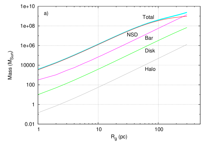
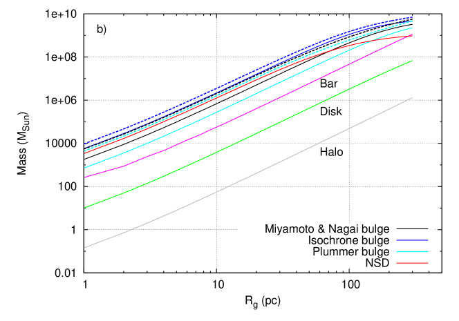
Figure 4: Mass enclosed in spheres of radius $R_{\text{g}}$ for the “bar + NSD” model (a) and when adding a classical bulge component to this model (b). The full mass profiles in panel (b) are shown as dashed lines; the color of each of these profiles coincides with the color of the contributing profile of the corresponding bulge model.

However, despite the influence of the NSD, the effect of potential asymmetry is noticeable: the orbits in Figure 3 are slightly elongated along the large axis of the bar. This is especially evident in the contours of the direction field that restrict regions with a four-fold field. Note that all the orbits constructed in this paper have the latter regions.

We tested the possible scale of deviations of the SMBH from the center of the NSC using a “naive” model, adding an NSC component to the “bar + NSD” model. Since the cluster shape is not spherically symmetric—the axis ratio is $c/a=0.71\pm 0.04$ ( Bland-Hawthorn & Gerhard 2016)—we did not consider the Plummer potential model, but adopted the Miyamoto & Nagai model (5) with parameter values of the half-light radius $a=4.2$ pc, $b=3$ pc and $M_{\text{NSC}}=1.8\times 10^{7}M_{\odot}$ (Bland-Hawthorn & Gerhard 2016). Even with the specified moderate mass of the NSC, at the nominal ${\mathbf{V}}^{0}(\text{BH})$ the deviations do not exceed 0.6 pc, which can be ignored at the present stage of the analysis.

It should be noted that possible oscillations of the gravitationally bound SMBH + NSC complex should hardly prevent the formation of a cuspy stellar distribution detected near Sgr A^∗(e.g. Gallego-Cano et al. 2020). Massive stars of the nuclear bulge are concentrated not only in the NSC, but also in several other clusters, including Sgr B2, Sgr B1, Sgr C and others (Launhardt et al. 2002). This means that the movement of these concentrations in the gravitational field does not interfere with star formation in them. A stellar cusp is then formed in the concentration in which there is the SMBH (Baumgardt et al. 2018), i.e. in NSC.

Note that the non-central start of the orbits increases the oscillation range. Taking into account irregular forces should lead to stochastization of motion, i.e., in general to greater deviations from the center. In this sense, the oscillation amplitudes obtained here are estimates from below. However, if a bulge component is still detected, it will, on the contrary, lead to stabilization of oscillations.

The obtained results suggest that at present it is impossible to exclude the non-centrality of position of the SMBH (Sgr A^∗) with a deviation from the Galactic barycenter only on the scale of about a dozen parsecs. The marginal significance of the SMBH peculiar radial velocity $V_{r}^{\text{LSR}}(\text{BH})$ (GRAVITY Collaboration et al. 2019) supports this possibility. The specified scale of SMBH deviation is still insignificant compared to the measurement precision and accuracy of $R_{0}$.