Leveraging the ALMA Atacama Compact Array for Cometary Science: An Interferometric Survey of Comet C/2015 ER61 (PanSTARRS) and Evidence for a Distributed Source of Carbon Monosulfide

Abstract

We report the first survey of molecular emission from cometary volatiles using standalone Atacama Compact Array (ACA) observations from the Atacama Large Millimeter/Submillimeter Array (ALMA) toward comet C/2015 ER61 (PanSTARRS) carried out on UT 2017 April 11 and 15, shortly after its April 4 outburst. These measurements of HCN, CS, CH₃OH, H₂CO, and HNC (along with continuum emission from dust) probed the inner coma of C/2015 ER61, revealing asymmetric outgassing and discerning parent from daughter/distributed source species. This work presents spectrally integrated flux maps, autocorrelation spectra, production rates, and parent scale lengths for each molecule and a stringent upper limit for CO. HCN is consistent with direct nucleus release in C/2015 ER61, whereas CS, H₂CO, HNC, and potentially CH₃OH are associated with distributed sources in the coma. Adopting a Haser model, parent scale lengths determined for H₂CO (L_p $\sim$ 2200 km) and HNC (L_p $\sim$ 3300 km) are consistent with previous work in comets, whereas significant extended source production (L_p $\sim$ 2000 km) is indicated for CS, suggesting production from an unknown parent in the coma. The continuum presents a point-source distribution with a flux density implying an excessively large nucleus, inconsistent with other estimates of the nucleus size. It is best explained by the thermal emission of slowly moving outburst ejectas, with total mass 5–8 $\times$ 10¹⁰ kg. These results demonstrate the power of the ACA for revealing the abundances, spatial distributions, and locations of molecular production for volatiles in moderately bright comets such as C/2015 ER61.

1 Introduction

Comets are among the most primitive remnants of solar system formation. Having accreted during the early stages of the protosolar disk, their initial composition should be indicative of the chemistry and thermodynamical processes present in the cold disk midplane where they formed (Bockelée-Morvan et al., 2004). Shortly after their formation, the migration of the giant planets gravitationally scattered comets across the solar system, placing many in their present day dynamical reservoirs, the Kuiper disk or the Oort cloud (Gomes et al., 2005; Morbidelli et al., 2005; Levison et al., 2011). Thus, comets have been stored in the cold outer solar system for the last $\sim$4.5 billion years in a relatively quiescent and unaltered state, preserved as “fossils” of solar system formation. Characterizing the composition of the comet nucleus, predominantly inferred through remote sensing of coma gases as comets pass through the inner solar system (heliocentric distances r_H $<$ 3 au), affords the opportunity to extract clues to solar system formation imprinted in their volatile composition.

Comet observations are interpreted using a Haser model (Haser, 1957) with coma volatiles identified as “parent” or “primary” (produced via direct sublimation from the nucleus and thus directly indicative of its composition), as “product” or “daughter” (produced by photolysis of gas-phase species in the coma), or as a distributed source (these cannot be explained by gas-phase processes and are likely formed from photo and thermal degradation of dust; Cottin & Fray, 2008). Such observations at multiple wavelengths have revealed extensive chemical diversity among the comet population independent of dynamical reservoir (e.g., A’Hearn et al., 1995; Crovisier et al., 2009; Cochran et al., 2012; Ootsubo et al., 2012; Dello Russo et al., 2016a). In particular, spectroscopy at millimeter/submillimeter (mm/sub-mm) wavelengths has detected a wealth of coma molecules through their rotational transitions, including those associated with direct nucleus sublimation in some comets (e.g., hydrogen cyanide, HCN, and methanol, CH₃OH), species associated with production from distributed coma sources (e.g., formaldehyde, H₂CO, and hydrogen isocyanide, HNC), and complex organic molecules (e.g., glycoaldehyde, C₂H₄O₂, and ethyl alcohol, C₂H₅OH; Bockelée-Morvan et al., 1994; Biver et al., 1999; Milam et al., 2006; Fray et al., 2006; Boissier et al., 2007; Lis et al., 2008; Biver, 2015). The advent of the Atacama Large Millimeter/Sub-millimeter Array (ALMA) has made mapping the 3D distribution of volatiles in the inner coma with exceptional spatial and spectral resolution possible, enabling unambiguous distinction between parent and product species (Cordiner et al., 2014; Bøgelund & Hogerheijde, 2017; Cordiner et al., 2017a, 2019, 2020). Although the long baselines (up to 16 km) provided by the 50 $\times$ 12 m antennas of the main ALMA array provide sensitive measurements at high angular resolution, they may resolve out the extended flux of most species and are blind to large-scale structures in the coma.

In contrast, the 12 $\times$ 7 m antennas of the ALMA Atacama Compact Array (ACA) are sensitive to extended molecular flux in the coma, providing short baselines between 9 and $\sim$50 m (corresponding to an angular resolution range from 3$\farcs$6 to 19$\farcs$3 at 345 GHz, equivalent to $\sim$3100 km – 16,700 km at the geocentric distance of C/2015 ER61 during our observations), that is available year-round as opposed to the vast configuration changes throughout the year for the 12 m array. Roth et al. (2021) reported the first detection of molecular emission in cometary atmospheres using the ACA, demonstrating rapidly varying, anisotropic CH₃OH production in comet 46P/Wirtanen via analysis of the spectral line profiles. Here we report the first comprehensive study of coma volatiles with the ALMA ACA in observations toward comet C/2015 ER61 (PanSTARRS) taken on UT 2017 April 11 and 15, shortly after its UT 2017 April 4 outburst. Secure detections of molecular emission were identified from HCN, CH₃OH, H₂CO, carbon monosulfide (CS), and HNC as well as continuum emission from dust. A stringent (3$\sigma$) upper limit was determined for carbon monoxide (CO) production. We report production rates, mixing ratios (relative to H₂O), spatial maps, and autocorrelation spectra of detected species. Section 2 discusses the observations and data analysis. Section 3 presents our results from these data. Section 4 discusses the distribution of each molecule and compares our results to comets characterized to date, and Section 5 analyzes continuum emission in C/2015 ER61 (PanSTARRS).

Table 1: Observing Log

Setting	UT Date	UT Time	tint	rH	$\Delta$	$\phi$	$\nu$	Nants	Baselines	$\theta$INT	$\theta$AC	PWV
			(minutes)	(au)	(au)	($\arcdeg$)	(GHz)		(m)	($\arcsec$)	($\arcsec$)	(mm)
1	2017 Apr 11	15:15–15:52	25	1.14	1.19	51	349.2	9	8.9–47.9	6.07$\times$2.56	28.35	1.14
2	2017 Apr 15	10:45–11:43	37	1.12	1.18	51	357.4	12	8.8–48.9	4.89$\times$2.31	27.71	2.39

Note. — T_int is the total on-source integration time. r_H, $\Delta$, and $\phi$ are the heliocentric distance, geocentric distance, and phase angle (Sun-comet-Earth), respectively, of ER61 at the time of observations. $\nu$ is the mean frequency of each instrumental setting. N_ants is the number of antennas utilized during each observation, with the range of baseline lengths indicated for each. $\theta$_INT is the angular resolution (Gaussian fit to the PSF) for the synthesized beam at $\nu$, $\theta$_AC is the angular resolution of the autocorrelation (7 m primary) beam at $\nu$, and PWV is the mean precipitable water vapor at zenith during the observations.

2 Observations and Data Reduction

Comet C/2015 ER61 (PanSTARRS; hereafter ER61) is a long-period comet from the Oort cloud (P $\sim$ 8600 yr, semi-major axis a = 715 au) that reached perihelion on UT 2017 May 14 (q = 1.04 au). Meech et al. (2017) reported CO₂-driven activity beginning near r_H = 8.8 au, followed by H₂O sublimation beginning near r_H = 5 au. Sekanina (2017) reported a major outburst in ER61 beginning on UT 2017 April 3.9, followed by splitting of the nucleus, and Saki et al. (2020) reported OCS and H₂O production rates in ER61 on UT 2017 May 12. We conducted pre-perihelion observations toward ER61 on UT 2017 April 11 and 15 during Cycle 4 using the ACA with the Band 7 receiver, covering frequencies between 342.3 and 364.4 GHz ($\lambda=$ 0.82 – 0.87 mm) in eight non-contiguous spectral windows ranging from 500 MHz wide (for the HCN and CO settings) to 1000 MHz wide (for the CS, HNC, CH₃OH, and H₂CO settings). The observing log is shown in Table 1. The comet position was tracked using JPL HORIZONS ephemerides (JPL #43). We used two correlator settings (one on each day) to simultaneously sample spectral lines from multiple molecules and the continuum. Weather conditions were fair (precipitable water vapor at zenith; zenith PWV = 1.14 – 2.29 mm). Quasar observations were used for bandpass and phase calibration. Neptune (on April 11) and Titan (on April 15) were used to calibrate ER61’s flux scale. The spatial scale (the range in semi-major and semi-minor axes of the synthesized beam) was 2$\farcs$31 – 6$\farcs$07 and the channel spacing was 122 kHz (for HCN and CO) and 244 kHz (for CS, HNC, CH₃OH, and H₂CO), leading to a spectral resolution of 0.10 – 0.20 km s^-1. The data were flagged, calibrated, and imaged using standard routines in CASA version 5.6.1 (McMullin et al., 2007). We deconvolved the point-spread function with the Högbom algorithm, using natural visibility weighting and a flux threshold of twice the rms noise in each image. For HNC, a 5$\arcsec$ Gaussian uv-taper was applied to the image to improve signal-to-noise. Self-calibration was applied to the continuum images to improve the dynamic range, resulting in an improvement from 3.4 to 11.7 on April 11 and from 4.7 to 10.2 on April 15. Self-calibration was not applied to the spectral lines. The deconvolved images were then convolved with a Gaussian fit to the PSF and corrected for the response of the ALMA primary beam. We transformed the images from astrometric coordinates to projected cometocentric distances, with the location of peak continuum flux chosen as the origin. The position of peak continuum flux (measured before the application of self-calibration) was in good agreement with the predicted ephemeris position.

Figure 1: (A)–(E). Autocorrelation spectra for HCN, CS, H₂CO, CH₃OH, and HNC in ER61 (blue dashed). Also shown are the corresponding interferometric spectra (black) for each transition. The spectral resolution is 122 kHz for HCN and 244 kHz for CS, HNC, CH₃OH, and H₂CO ($\sim$0.10–0.20 km s^-1). Note the differing scales for the y-axis for each beam.

2.1 Autocorrelation Spectra

To recover extended flux that may have been resolved out by the ACA, we extracted autocorrelation spectra at the expected frequency for each transition detected in the imaging as well as for the CO (J = 3–2) transition (not detected in imaging). These autocorrelation spectra are collected for each antenna simultaneously with the cross-correlation spectra, but are flagged (discarded) in order to process the interferometric data. We recovered, extracted, and calibrated the autocorrelation spectra on each date as in Cordiner et al. (2019, 2020). A 20% uncertainty in flux was assumed to account for uncertainties in the extraction process (e.g., opacity, T_sys, background subtraction, beam efficiencies). The autocorrelation spectra were corrected for a main beam efficiency, $\eta$_MB = 0.75, as in Cordiner et al. (2020). Figure 1 shows autocorrelation spectra for each detected species along with the corresponding interferometric spectra extracted from the nucleus-centered beam.

3 Results

We detected molecular emission from HCN, CS, CH₃OH, H₂CO, and HNC as well as continuum emission from dust/icy grains in the coma of ER61, and derived a sensitive upper limit for CO. We modeled molecular line emission using a three-dimensional radiative transfer method based on the Line Modeling Engine (LIME; Brinch & Hogerheijde, 2010) adapted for cometary atmospheres, including a full non-LTE treatment of coma gases, collisions with H₂O and electrons, and pumping by solar radiation (Appendix A; see Cordiner et al., 2019, for further details). Our models were run through the CASA “simobserve” tool to mimic the effects of the ACA using the exact antenna configuration and hour angle range of our observations. Photodissociation rates for all molecules were adopted from Huebner & Mukherjee (2015) with the exception of CS (Boissier et al., 2007). Detected spectral lines, including upper-state energies (E_u), calculated production rates (Q), parent scale lengths (L_p), and integrated fluxes are listed in Table 2.

Table 2: Molecular Composition of C/2015 ER61 (PanSTARRS)

Species	Transition	Eu	$\int T_{B}\,dv$a	$\int T_{B}\,dv$b	Lpc	Qd	Qx/QH2Oe	Range in Cometsf
		(K)	(K km s-1)	(K km s-1)	(km)	(1025 mol s-1)	(%)	(%)
UT 2017 April 11, rH = 1.14 au, $\Delta$ = 1.19 au
HCN	4–3	25.5	3.69 $\pm$ 0.06	0.26 $\pm$ 0.05	$50^{+50}_{-30}$	8.6 $\pm$ 0.3	0.072	0.08–0.25
CS	7–6	65.8	0.25 $\pm$ 0.05	0.082 $\pm$ 0.016	$2000^{+3100}_{-1200}$	7.4 $\pm$ 0.9	0.061	0.02–0.20
CO	3–2	33.2	$<$ 0.147 (3$\sigma$)	$<$ 0.009 (3$\sigma$)	$\cdot\cdot\cdot$	$<$ 191 (3$\sigma$)	$<$ 1.6 (3$\sigma$)	0.3–23
UT 2017 April 15, rH = 1.12 au, $\Delta$ = 1.18 au
H2CO	$5_{15}$–$4_{14}$	62.4	0.58 $\pm$ 0.04	0.085 $\pm$ 0.017	$2200^{+1100}_{-800}$	37 $\pm$ 3	0.31	0.13-1.4
CH3OH	$1_{1}$–$0_{0}$ $A^{+}$	16.8	0.40 $\pm$ 0.05	0.084 $\pm$ 0.017	$300^{+1400}_{-260}$	230 $\pm$ 88	1.9	0.6–6.2
HNC	4–3	43.5	0.36 $\pm$ 0.07	0.046 $\pm$ 0.009	$3300^{+19,700}_{-2800}$	0.82 $\pm$ 0.17	0.007	0.002–0.035

Note. — ^a Spectrally integrated flux extracted from the interferometric nucleus-centered beam at the position of peak continuum flux. ^b Spectrally integrated flux extracted from autocorrelation spectra. ^c Parent scale length derived from interferometric visibility modeling. ^d Molecular production rate calculated using the best-fit parent scale length. ^e Mixing ratio with respect to H₂O with Q(H₂O) = 1.2 $\times 10^{29}$ s^-1 as measured by Saki et al. (2021) on UT 2017 April 15. ^f Range of mixing ratios in comets (Dello Russo et al., 2016a; Bockelée-Morvan & Biver, 2017).

3.1 Interferometric Molecular Maps, Extracted Spectra

Figures 2 and 3 show observed spectra and spectrally integrated flux maps for each species detected with the ACA in ER61. Differences are evident between the emissions of individual molecules as well as dust. ER61 displays a compact dust continuum that falls off within a few thousand km of the nucleus, whereas molecular emission extends up to greater nucleocentric distances. The distribution of HCN is compact and consistent with that expected for a parent species, whereas those of CS and HNC are more extended and consistent with a product or distributed source distribution. On April 11, the continuum peak is offset from the HCN peak by $\sim$1200 km to the southwest (i.e., anti-sunward), whereas on April 15 the continuum and molecular emission peaks are better aligned, with the continuum peaking $\sim$850 km to the northeast (sunward) of the H₂CO emission. The continuum emission is unresolved and further discussed in Section 5. We performed a detailed analysis of the parentage of each species (Section 4). Additionally, the extracted spectra are all indicative of a red-shifted peak, suggesting asymmetries in outgassing along the Sun–comet line (Section 3.3).

Figure 2: (A)–(C). Spectrally integrated flux maps for HCN, CS, and continuum in ER61 on UT 2017 April 11. Contour intervals in each map are 20% of the peak. The rms noise ($\sigma$, mJy beam^-1 km s^-1) and contour spacing, $\delta$, for each map are: (A) HCN: $\sigma$ = 230, $\delta$ = 5.2$\sigma$, (B) CS: $\sigma$ = 120, $\delta$ = 1.1$\sigma$, and (C) Continuum: $\sigma$ = 4.4 mJy beam^-1, $\delta$ = 3.1$\sigma$. Sizes and orientations of the synthesized beam (6$\farcs$07$\times$2$\farcs$56) are indicated in the lower left corner of each panel. The comet’s illumination phase ($\phi\sim$ 51$\arcdeg$), as well as the direction of the Sun and dust trail, are indicated in the lower right. The black cross indicates the position of the peak continuum flux. A spectral line profile taken at the peak of emission is shown in the upper right.

Figure 3: (A)–(D). Spectrally integrated flux maps for CH₃OH, H₂CO, HNC, and continuum on UT 2017 April 15, with traces and labels as in Figure 2. Contour intervals in each map are 20% of the peak. The rms noise ($\sigma$, mJy beam^-1 km s^-1) and contour spacing, $\delta$, for each map are: (A) CH₃OH: $\sigma$ = 69, $\delta$ = 1.9$\sigma$, (B) H₂CO: $\sigma$ = 49, $\delta$ = 4.3$\sigma$, (C) HNC: $\sigma$ = 138, $\delta$ = 0.61$\sigma$, and (D) Continuum: $\sigma$ = 3.3 mJy beam^-1, $\delta$ = 9.0$\sigma$. A spectral line profile taken at the peak of emission is shown in the upper right.

The complexity of ER61’s coma as captured by the ACA is further revealed in velocity channel maps for each molecule (Figure 4). The spatial extents of emissions for each molecule are not constant across velocity space. Whereas the overall shape of HCN and H₂CO emissions are relatively consistent across a range of cometocentric velocities, CS and HNC (and to a lesser extent, CH₃OH) exhibit asymmetric structures varying in extent and shape across a relatively narrow range of velocity space.

Figure 4: (A)–(E). Velocity channel maps for (A) HCN, (B) CS, (C) H₂CO, (D) CH₃OH, and (D) HNC in ER61. Each contour level is 20% of the peak flux across all channels. The cometocentric velocity of each channel is indicated in the bottom for each map, and the peak continuum flux position is indicated by a black cross.

3.2 Rotational and Temperature

We detected emission from one CH₃OH transition on April 11 and three additional CH₃OH transitions on April 15. We constrained the coma rotational temperature along the line of sight using the rotational diagram method (Bockelée-Morvan et al., 1994) for both the interferometric and autocorrelation spectra. Our results indicate a best-fit rotational temperature T_rot = 61 $\pm$ 5 K for the interferometric nucleus-centered spectra and T_rot = 58 $\pm$ 4 K for the autocorrelation spectra. Table 3 provides line transitions and integrated fluxes for each CH₃OH line used in the analysis and Figure 5 shows our CH₃OH rotational diagrams and best-fit lines.

Table 3: CH₃OH Lines Detected in C/2015 ER61 (PanSTARRS)

Transition	Frequency	Eu	$\int T_{B}\,dv$a	$\int T_{B}\,dv$b
(J’K’–JK	(GHz)	(K)	(K km s-1)	(K km s-1)
Setting 1, UT 2017 April 11, rH = 1.14 au, $\Delta$ = 1.19 au
$13_{1}$–$13_{0}A^{-+}$	342.730	227.5	0.18 $\pm$ 0.04	0.025 $\pm$ 0.005
Setting 2, UT 2017 April 15, rH = 1.12 au, $\Delta$ = 1.18 au
$1_{1}$–$0_{0}$ $A^{+}$	350.905	16.8	0.40 $\pm$ 0.05	0.084 $\pm$ 0.017
$4_{0}$–$3_{-1}$ $E$	350.687	36.3	0.34 $\pm$ 0.04	0.041 $\pm$ 0.008
$7_{2}$–$6_{1}$ $E$	363.739	87.3	0.35 $\pm$ 0.10	0.061 $\pm$ 0.012

Note. — ^a Spectrally integrated flux of spectra extracted from a nucleus-centered beam at the position of peak continuum flux. ^b Spectrally integrated flux of autocorrelation spectra.

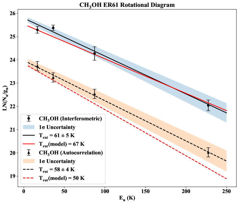
Figure 5: Rotational diagram of the CH₃OH J_K = $13_{1}$–$13_{0}$ $A^{-+}$ transition in ER61 on UT 2017 April 11 and the J_K = $1_{1}$–$0_{0}$ $A^{+}$, J_K = $4_{0}$–$3_{-1}$ $E$, and J_K = $7_{2}$–$6_{1}$ $E$ transitions on UT 2017 April 15 for interferometric nucleus-centered (black circles) and autocorrelation (black triangles) spectra. The best-fit lines, corresponding to T_rot = 61 $\pm$ 5 K for the interferometric spectra and 58 $\pm$ 4 K for the autocorrelation spectra are shown as well as the 1$\sigma$ uncertainty in the fits (shaded areas). Also shown are the rotational diagrams for the best-fit non-LTE models for T_kin = 75 K (interferometric spectra, solid red line) and for T_kin = 88 K (autocorrelation spectra, dashed red line). Note that the interferometric data are extracted from the nucleus-centered beam whereas the autocorrelation data are from the considerably larger autocorrelation beam (Table 1).

3.3 Expansion Velocities, Kinetic Temperature, and Asymmetric Outgassing

We derived expansion velocities, coma kinetic temperatures, and outgassing asymmetry factors for each molecule by performing nonlinear least-squares fits of our radiative transfer models to extracted interferometric and autocorrelation spectral line profiles. Table 4 lists our results for the strongest line for each detected species and Figure 6 shows our extracted spectra and best-fit models for the interferometric spectra.

3.3.1 Kinetic Temperature

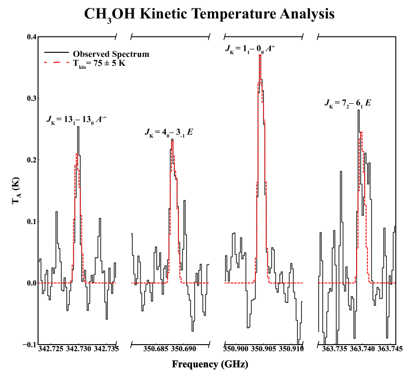
Figure 7: Extracted interferometric spectra and best-fit kinetic temperature model (T_kin = 75 $\pm$ 5 K) for the CH₃OH J_K = $13_{1}$–$13_{0}$ $A^{-+}$ transition in ER61 on UT 2017 April 11 and the J_K = $1_{1}$–$0_{0}$ $A^{+}$, J_K = $4_{0}$–$3_{-1}$ $E$, and J_K = $7_{2}$–$6_{1}$ $E$ transitions on UT 2017 April 15. Spectra were extracted from the nucleus-centered beam.

We determined the coma kinetic temperature by fitting full non-LTE models to all four detected CH₃OH lines simultaneously for both the interferometric and autocorrelation spectra. We assumed that the collision rate between CH₃OH and H₂O is the same as that with H₂ (taken from the LAMDA database; Schöier et al., 2005; Rabli & Flower, 2010). Calculating formal CH₃OH–H₂O collision rates is the subject of a future work and beyond the scope of this paper. For the interferometric nucleus-centered spectra, the best-fit kinetic temperature, T_kin = 75 $\pm$ 5 K, is higher than the derived rotational temperature (61 $\pm$ 5 K). Similarly, for the autocorrelation spectra, the best-fit kinetic temperature is T_kin = 88 $\pm$ 8 K, and is significantly higher than the rotational temperature (58 $\pm$ 4 K). As these two measurements are in formal agreement, we assumed a kinetic temperature T_kin = 78 K (the weighted average of the best-fit kinetic temperatures) when modeling all other molecules in ER61. Production rates derived by setting T_kin = T_rot (61 K) are in formal agreement with those derived by setting T_kin = 78 K. Figure 7 shows extracted spectra and our best-fit model for each CH₃OH line.

3.3.2 Expansion Velocities and Asymmetric Outgassing

Uniform outgassing vs. hemispheric asymmetry along the Sun–comet vector were considered when fitting the observations for each molecule, beginning with the HCN (J = 4 – 3) transition, the strongest in our dataset. Assuming isotropic outgassing, our best-fit radiative transfer model finds v_exp = 0.51 $\pm$ 0.02 km s^-1, with a reduced chi-square ($\chi^{2}_{r}$) of 2.61, corresponding to P = 0.0 (where P is the probability that the model differs from the observations due to random noise). Instead, assuming hemispheric asymmetry along the Sun–comet vector, our best-fitting model indicates an expansion velocity v_exp(1) = 0.60 $\pm$ 0.01 km s^-1 in the sunward hemisphere and v_exp(2) = 0.42 $\pm$ 0.01 km s^-1 in the anti-sunward hemisphere, with a ratio of sunward to anti-sunward production rates of 1.30 $\pm$ 0.05. For the asymmetric model, we find $\chi^{2}_{r}$ = 1.005, corresponding to P = 0.47; therefore, the asymmetric outgassing model is strongly favored.

Expansion velocities and asymmetry factors for CS, CH₃OH, and HNC are consistent with those for HCN within uncertainty for the interferometric spectra, suggesting similar outgassing for each species and/or their parents. The exception was H₂CO, where the best-fitting asymmetry factor of sunward to anti-sunward production rates was 0.51 $\pm$ 0.09 (Table 4). This suggests increased H₂CO production in the anti-sunward hemisphere of ER61.

The slower expansion velocity in the anti-sunward hemisphere combined with the asymmetry factor (1.30), indicating higher HCN production in the sunward hemisphere, helps to explain the red-shifted line profile, as HCN molecules outgassing from the anti-sunward side would have remained in the ACA beam for longer than those from the sunward side. Conversely, for H₂CO, the expansion velocities in each hemisphere are in formal agreement, yet the asymmetry factor (0.51) indicates increased H₂CO production in the anti-sunward hemisphere. This helps explain how the distinct H₂CO outgassing pattern (compared to all other species) still results in a red-shifted line profile – H₂CO molecules remained in the ACA beam for roughly the same time in each hemisphere, yet there was a greater amount of H₂CO production in the anti-sunward (red) hemisphere.

Compared with quantities derived for the interferometric spectra, the expansion velocities derived from the autocorrelation spectra were in general slightly larger, with the HCN expansion velocities being most similar in both cases and the H₂CO, CH₃OH, and CS expansion velocities showing significant differences. Asymmetry factors (the ratio of sunward to anti-sunward production) were similar for all molecules except CS, for which the asymmetry factor is a factor of two higher for the interferometric spectra compared to the autocorrelation spectra, suggesting increased CS production in the anti-sunward hemisphere of ER61 on large angular scales. Combined with the non-uniform coma structures displayed in the channel maps of each molecule (Figure 4), these results highlight the complex nature of ER61’s coma.

Table 4: Expansion Velocities, Kinetic Temperature, and Asymmetry Factors in C/2015 ER61 (PanSTARRS)

Molecule	Tkina	vexp(1)b	vexp(2)c	Q1/Q2d	$\chi^{2}$re	Pf
(Transition)	(K)	(km s-1)	(km s-1)
Interferometric Spectra
HCN (4–3)	(78)	0.60 $\pm$ 0.01	0.42 $\pm$ 0.01	1.30 $\pm$ 0.05	1.001	0.46
		0.51 $\pm$ 0.02g		$\cdot\cdot\cdot$	2.610g	0.00g
CS (7–6)	(78)	0.55 $\pm$ 0.08	0.41 $\pm$ 0.06	1.2 $\pm$ 0.4	0.907	0.78
H2CO ($5_{15}$–$4_{14}$)	(78)	0.54 $\pm$ 0.04	0.50 $\pm$ 0.02	0.51 $\pm$ 0.09	1.073	0.25
	(78)	(0.60)	(0.42)	(1.30)	1.518	0.00h
CH3OH ($1_{1}$–$0_{0}$ $A^{+}$)	75 $\pm$ 5	0.56 $\pm$ 0.07	0.37 $\pm$ 0.06	1.2 $\pm$ 0.4	1.043	0.34
HNC (4–3)	(78)	0.9 $\pm$ 0.3	0.4 $\pm$ 0.1	1.1 $\pm$ 0.6	0.948	0.65
	(78)	(0.60)	(0.42)	(1.30)	0.967	0.60
Autocorrelation Spectra
HCN (4–3)	(78)	0.65 $\pm$ 0.01	0.50 $\pm$ 0.01	1.19 $\pm$ 0.03	1.377	0.001
CS (7–6)	(78)	0.68 $\pm$ 0.05	0.60 $\pm$ 0.03	0.61 $\pm$ 0.07	1.300	0.033
H2CO ($5_{15}$–$4_{14}$)	(78)	0.84 $\pm$ 0.08	0.48 $\pm$ 0.04	0.7 $\pm$ 0.1	1.2988	0.032
CH3OH ($1_{1}$–$0_{0}$ $A^{+}$)	88 $\pm$ 8	0.76 $\pm$ 0.02	0.63 $\pm$ 0.03	1.7 $\pm$ 0.2	1.306	0.002
HNC (4–3)	(78)	0.9 $\pm$ 0.2	0.6 $\pm$ 0.1	1.4 $\pm$ 0.5	1.064	0.317

Note. — ^a Coma kinetic temperature. We assumed the weighted average of the kinetic temperatures measured from CH₃OH interferometric and autocorrelation spectra when modeling other species. Values in parentheses are assumed. ^b Expansion velocity in the sunward hemisphere. ^c Expansion velocity in the anti-sunward hemisphere. ^d Asymmetry factor: ratio of production rates in the sunward vs. anti-sunward hemisphere. ^e Reduced $\chi^{2}$ of the model fit. ^f P-value of the fit: the probability that the difference between the model and the observations is due to random noise. ^g Expansion velocity, reduced $\chi^{2}$, and P-value for the best-fit HCN model assuming isotropic outgassing. ^h Reduced $\chi^{2}$ and P-value for H₂CO when assuming the expansion velocities and asymmetry factor found for HCN, indicating that increased anti-sunward production is statistically strongly favored for H₂CO.

Figure 6: (A)–(E). Extracted interferometric spectra and best-fit models for (A) HCN, (B) CS, (C) H₂CO, (D) CH₃OH, and (E) HNC. Spectra were extracted from the nucleus-centered beam.

3.4 CO Autocorrelation Spectra

Emission from the CO (J = 3 – 2) transition near 345.795 GHz was not confirmed in our interferometric maps. To constrain CO production in ER61, we extracted a spectrum from the expected position of the nucleus in the CO map. CO was assumed to be outgassing with the same expansion velocities and asymmetry factor as HCN. Integrating from -1.5 km s^-1 to +1.5 km s^-1 (the width of the HCN (J = 4 – 3) line), a 3$\sigma$ upper limit for the integrated intensity of $<$ 147 mK km s^-1 was derived, corresponding to a production rate Q(CO) $<$ 2.3 $\times$ 10²⁷ mol s^-1 and a mixing ratio CO/H₂O $<$ 1.96%.

In order to improve sensitivity and derive a more stringent upper limit for CO, we extracted autocorrelation spectra as in Section 2.1. CO was not detected in the autocorrelation spectra. Based on the flux at the position of the CO (J = 3 – 2) transition in the autocorrelation spectra, we constrained a 3$\sigma$ upper limit for the integrated intensity of $<$ 9 mK km s^-1, corresponding to a production rate Q(CO) $<$ 1.91 x 10²⁷ mol s^-1 and a mixing ratio CO/H₂O $<$ 1.59%. CO mixing ratios span a wide range in measured Oort cloud comets (0.4 – 23%) and much narrower range in the fewer Jupiter-family comets for which this molecule has been detected (0.3 – 4.3%), making the upper limit in ER61 consistent with depleted Oort cloud comets and more similar to Jupiter-family comets (Dello Russo et al., 2016a; Bockelée-Morvan & Biver, 2017). This may suggest that ER61 formed in an area of the protosolar disk where ices suffered enhanced processing before incorporation into its nucleus compared to those from CO-rich Oort cloud comets.

4 Production Rates and Molecular Distribution

We calculated molecular production rates and parent scale lengths for all detected species. Although our measurements did not sample H₂O, we calculated mixing ratios to facilitate comparisons with other comets. We adopted Q(H₂O) = 1.2 $\times$ $10^{29}$ s^-1 based on near-infrared measurements of H₂O on UT 2017 April 15, coinciding with the second date of our ACA study (Saki et al., 2021). Following the methods of Boissier et al. (2007), we performed nonlinear least-squares fits of models generated over a range of production rates and parent scale lengths to the real part of the interferometric and autocorrelation visibilities as a function of projected baseline for each molecule. Using a Haser model (Haser, 1957), we determined the distribution of each trace species using:

$$n_{d}(r)=\frac{Q}{4\pi v_{exp}r^{2}}\frac{\frac{v_{exp}}{\beta_{d}}}{\frac{v_{exp}}{\beta_{d}}-L_{p}}\left[\exp{\left(-\frac{r\beta_{d}}{v_{exp}}\right)}-\exp{\left(-\frac{r}{L_{p}}\right)}\right],$$ (1)

where Q is the production rate (molecules s^-1), v_exp is the expansion velocity (km s^-1), $\beta$_d is the photodissociation rate (s^-1), and L_p is the parent scale length (km), with Q, v_exp, and L_p allowed to vary as free parameters.

We used the expansion velocities, asymmetry factors, and kinetic temperatures listed in Table 4 for each molecule when generating synthetic visibilities for each component of the model (interferometric and autocorrelation). A single L_p and Q was used to fit both components (interferometric and autocorrelation). Figures 8 and 9 show the observed visibilities with best-fit models, enabling us to discern parent species from product and to determine the mechanism of molecular production for each species in ER61. We detail our results for each molecule in turn.

Figure 8: (A)–(B). Real part of the observed visibility amplitude vs. projected baseline length for HCN and CS in ER61 on UT 2017 April 11. Modeled visibility curves for various parent scale lengths (L_p) are shown with the best-fit model for each molecule plotted in red (solid) and $\pm$1$\sigma$ uncertainties in L_p shown in green (dotted) and purple (dash–dotted). A parent molecule model (L_p = 0 km, orange, dashed) is also shown for comparison. Interpolation is used between the zero-point spacing and shortest ACA baseline.

Figure 9: (A)–(C). Real part of the observed visibility amplitude vs. projected baseline length for H₂CO, CH₃OH, and HNC in ER61 on UT 2017 April 15, with traces and labels as in Figure 8. Interpolation is used between the zero-point spacing and shortest ACA baseline.

4.1 HCN

We detected emission from the HCN (J = 4 – 3) transition near 354.505 GHz. We find a best-fit parent scale length L_p = $50^{+50}_{-30}$ km, consistent with HCN production at or very close to the nucleus (Figure 8). This is consistent with results from previous ALMA studies using the 12 m array (Cordiner et al., 2014) indicating HCN production as a parent species, although our ACA measurements lack the longer baselines necessary to explicitly confirm HCN release at the nucleus or in the very inner coma. The production rate, Q(HCN) = (8.6 $\pm$ 0.3) $\times$ $10^{25}$ s^-1, corresponds to an abundance relative to H₂O of 0.072%, a value in the low range of HCN abundances measured in comets at radio wavelengths (Bockelée-Morvan & Biver, 2017).

4.2 CS

Previous work for other comets has indicated that CS is a product species produced in the inner coma, ranging in abundance from 0.02 – 0.20% with respect to H₂O. Although short-lived CS₂ has been suggested, a precursor has never been conclusively identified (Feldman et al., 2004; Boissier et al., 2007; Bøgelund & Hogerheijde, 2017). Our visibility modeling is well aligned with CS as a product species, with parent scale length L_p = $2000^{+3100}_{-1200}$ km, corresponding to a photodissociation rate $\beta$ = $(3.57^{+5.36}_{-2.17})$ $\times$ $10^{-4}$ s^-1 at r_H = 1 au. This is considerably longer than the photodissociation rate expected for CS₂ (2.93 $\times$ $10^{-3}$ s^-1 at r_H = 1 au), and suggests the presence of an unidentified parent for CS production in ER61. Although CS production from CS₂ in the very inner coma cannot be ruled out by our measurements, Figure 8 demonstrates that CS₂ photolysis cannot account for the significant extended production of CS revealed in ER61. The production rate, Q(CS) = (7.4 $\pm$ 0.9) $\times$ $10^{25}$ s^-1, corresponds to an abundance relative to H₂O of 0.061%, consistent with average abundances in comets (Bockelée-Morvan & Biver, 2017).

The presence of a distributed source of CS in the coma would not be not surprising in the context of other species found in comets (e.g., H₂CO, HNC) as well as unresolved questions regarding the sulfur inventory of various astronomical sources. An observed depletion of gas-phase sulfur-bearing species in dense clouds and star-forming regions along with a depletion of ice-phase sulfur-bearing molecules in the interstellar medium has resulted in a search for “missing sulfur” (Mifsud et al., 2021). Similar to the unknown refractory parent suggested for H₂CO (Section 4.3) and the refractory ammonium salts identified as potential reservoirs for the “missing nitrogen” in comets (Altwegg et al., 2020), an unidentified refractory sulfur-bearing component has been suggested to address the observed sulfur depletion. A distributed, refractory source for CS would be consistent with the observed heliocentric dependence of CS production (Cottin & Fray, 2008, and references therein), which cannot be explained by photolysis of CS₂, as well as the organo-sulfur molecules identified alongside the ammonium salts in comet 67P/Churyumov–Gerasimenko by Rosetta (Altwegg et al., 2020). Thus, it is possible that an unidentified refractory sulfur-bearing parent may be responsible for the extended CS production in ER61, analogous to those suspected for H₂CO and HNC.

On the other hand, the photolysis of gas-phase species provides another potential avenue for extended CS production. Jackson et al. (1986) examined potential parents of CS in comet IRAS-Araki-Alcock 1983d, for which the CS parent scale length was $\sim$300 km. HNCS (thiocyanic acid) was discounted as only producing the HNC, H, S, and NCS fragments. CH₃SH (methanethiol) would require cleaving four H’s which would likely result in poor yields. Furthermore, CH₃SH dissociates to CH₃S + H and CH₃ + SH rapidly (calculated as $\sim$500 s at r_H = 1 au; Huebner & Mukherjee, 2015). Perhaps the most compatible gas-phase precursor previously detected in comets is H₂CS (thioformaldehyde). Ranging from 0.009 – 0.09% (Bockelée-Morvan & Biver, 2017) in measured comets, H₂CS was associated with coma production as well as direct nucleus release in comet 67P/Churyumov–Gerasimenko by Rosetta (Calmonte et al., 2016). Although its lifetime in the solar radiation field has not been published, it may be similar to H₂CO (Jackson et al., 1986), suggesting a lifetime of $\sim$5600 s at the heliocentric distance of ER61 and a scale length of $\sim$3400 km, in good agreement with our derived L_p of 2000${}^{+3100}_{-1200}$ km for CS. Although the observed abundance range of H₂CS in comets encompasses that for CS in ER61 reported here, it is too low to account for comets with higher CS abundances (up to 0.2%).

Clearly, the identity of the parent for extended CS production in ER61 is unresolved. The lack of strong correlation with a specific parent species highlights the need for laboratory measurements of potential CS parents. This includes studies of not only the photodissociation rates but of products and branching ratios for incorporation into analytical and chemical models.

4.3 H₂CO

We detected emission from the H₂CO (J_KaKc = $5_{15}$ – $4_{14}$) transition near 351.768 GHz. Although H₂CO has been primarily associated with nucleus sources based on observations of the inner coma at near-infrared wavelengths (Dello Russo et al., 2016a), measurements from the Neutral Mass Spectrometer on board the Giotto spacecraft indicated distributed source production of H₂CO in comet 1P/Halley (Meier et al., 1993). Furthermore, millimeter studies have indicated H₂CO production from an unknown parent source with a scale length of 6800 km at 1 au (Biver et al., 1999; Bockelée-Morvan et al., 2000; Milam et al., 2006), and ALMA observations of the inner coma suggest a scale length of 1000 – 5000 km (Cordiner et al., 2014, 2017b). The H₂CO visibilities in ER61 are similarly consistent with distributed source production, with a best-fit parent scale length L_p = $2200^{+1100}_{-800}$ km at r_H $\sim$ 1.12 au. Our production rate, Q(H₂CO) = (3.7 $\pm$ 0.3) $\times$ 10²⁶ s^-1, corresponds to an H₂CO mixing ratio of 0.31%, consistent with average values in comets (Dello Russo et al., 2016a; Bockelée-Morvan & Biver, 2017).

Our measured L_p is consistent with the parent scale length L_p = $1200^{+1200}_{-400}$ km found in C/2012 F6 (Lemmon) at r_H = 1.48 au using the 12 m array, but considerably larger than the 280 $\pm$ 50 km parent scale length found in C/2012 S1 (ISON) at r_H = 0.54 au (Cordiner et al., 2014). Taking into account the greatly increased solar radiation at the small r_H of S1 (ISON) compared to ER61 and F6 (Lemmon), these differing parent scale lengths are all compatible with optically thin photodissociation of a parent molecule in uniform outflow.

On the other hand, a comparison of the derived photodissociation rates at r_H = 1 au for all three comets (Table 5) indicates a considerably longer photodissociation scale for H₂CO in ER61 than for S1 (ISON) or F6 (Lemmon). We derived these “effective” parent photodissociation rates at r_H = 1 au by correcting L_p for the gas expansion velocity (v_exp) reported for each comet and scaling by the r_H of the comet as r_H². Assuming v_exp = 0.8 km s^-1 at r_H = 1 au, the parent scale length of 6800 km mentioned above would correspond to $\beta$ = 1.17 $\times$ $10^{-4}$ s^-1, in better agreement with the value derived for ER61 than that for S1 (ISON) or F6 (Lemmon). The differences seen among comets may indicate non-Haser behavior for the unidentified H₂CO parent, and emphasize the work remaining in understanding the H₂CO photochemistry in comets.

Table 5: Parent Photodissociaton Rates at r_H = 1 au in Comets Studied with ALMA

Molecule	ER61	C/2012 S1 (ISON)	C/2012 F6 (Lemmon)
HCN	($1.55^{+2.34}_{-0.78}$) $\times$ $10^{-2}$	$>5.8$ $\times$ $10^{-3}$	$>3.05$ $\times$ $10^{-2}$
CS	($3.57^{+5.36}_{-2.17})$ $\times$ $10^{-4}$	($1.46^{+0.47}_{-0.29})$ $\times$ $10^{-3}$	$\cdot\cdot\cdot$
H2CO	($3.08^{+1.76}_{-1.03})$ $\times$ $10^{-4}$	($1.04^{+0.23}_{-0.16})$ $\times$ $10^{-3}$	($1.26^{+0.63}_{-0.63})$ $\times$ $10^{-3}$
HNC	($2.28^{+12.7}_{-1.95})$ $\times$ 10-4	($4.16^{+5.55}_{-2.54})$ $\times$ $10^{-4}$	$\cdot\cdot\cdot$

Note. — Photodissociation rate (s^-1) corrected for v_exp and r_H at the time of the observations. Rates for ISON and Lemmon taken from Cordiner et al. (2014) except for CS (Bøgelund & Hogerheijde, 2017).

4.4 CH₃OH

As detailed in Section 3.2, we detected multiple transitions of CH₃OH in ER61. The visibilities are best fit with a parent scale length L_p = $300^{+1400}_{-260}$ km. The uncertainty in the production rate, Q(CH₃OH) = (2.3 $\pm$ 0.9) $\times$ $10^{27}$ s^-1, reflects the significant uncertainty in L_p rather than the spectral line (detected at 8$\sigma$; Table 2), and corresponds to a mixing ratio of $\sim$1.9%.

The half-width at half-maximum of the ACA beam on April 15 corresponded to nucleocentric distances of 988 km $\times$ 2092 km, so it is possible that an unresolved distributed source of CH₃OH production was captured by our measurements. Despite its high nominal value, it is important to note that the lower bound on L_p is consistent with CH₃OH production at or very near to the nucleus, and our measurements cannot decisively distinguish between direct nucleus release and distributed source production of CH₃OH in ER61.

If CH₃OH was indeed produced from distributed sources in ER61, it may have been from icy CH₃OH-coated grains. Icy grain release of CH₃OH was indicated for comet 103P/Hartley 2 (Drahus et al., 2012; Boissier et al., 2014) as well as for comet 46P/Wirtanen (Bonev et al., 2021; Roth et al., 2021), although these were both “hyperactive” comets displaying significant production of H₂O from icy grain release (e.g., Lis et al., 2019, and references therein). Although ER61 was not a hyperactive comet, as noted in Section 5, it had undergone a significant outburst 11.5 days prior and was likely in the process of nucleus fragmentation during our observations (Sekanina, 2017). This nucleus fragmentation process may have liberated icy CH₃OH-coated grains into the coma, from which CH₃OH sublimed and added to the overall production rate.

4.5 HNC

Finally, we detected emission from the HNC (J = 4 – 3) transition near 362.630 GHz. Early studies of HNC in C/1995 O1 (Hale–Bopp) were inconsistent with nucleus production (Irvine et al., 1998), and recent work with ALMA in C/2012 S1 (ISON) suggests that HNC is produced via degradation of complex organics, perhaps HCN polymers (Cordiner et al., 2017b). Our best-fit parent scale length is L_p = $3300^{+19,700}_{-2800}$ km, which is consistent with a dominant coma source for this molecule. We derive a production rate Q(HNC) = (8.2 $\pm$ 1.7) $\times$ 10²⁴ s^-1, which corresponds to an HNC mixing ratio of 0.007% with respect to H₂O, and Q(HNC)/Q(HCN) = 0.094 $\pm$ 0.023, about twice as high as the value of 0.05 predicted by the heliocentric dependence of Q(HNC)/Q(HCN) in comets found by Lis et al. (2008).

5 Analysis of Continuum Emission in ER61

The continuum detected on April 11 and 15 is compact and characteristic of unresolved thermal emission (Figures 2 and 3) from a source much smaller than the interferometric beam ($\sim$ 2100 $\times$ 4700 km). Unlike the molecular line emission (Figures 8 and 9) and as expected for an unresolved source, the visibilities for the continuum remain constant over the range of projected baseline lengths (9–49 m; Figure 10), with mean values $S_{\lambda}$ = 37 $\pm$ 5 mJy and 70 $\pm$ 4 mJy for April 11 and 15, respectively. The detected 0.85 mm emission is likely due to the thermal emission of a compact cloud of dust particles in the near-nucleus coma. Indeed, based on the Near-Earth Asteroid Thermal Model (NEATM; Harris, 1998) with a beaming factor $\eta$ = 0.7 and a bolometric emissivity of 0.8 (Boissier et al., 2011), the detected flux density of 37 mJy at 350 GHz on April 11 would imply an excessively large 19 km radius nucleus, inconsistent with other estimates of the nucleus size. Pre-discovery observations on 2014 February 12, when the comet was at 11.33 au from the Sun, place an upper limit on the nucleus radius of 7–10 km (Meech et al., 2017). In addition, both Pan-STARRS1 and WISE photometric observations performed in 2015, when the comet was at distances $\geq$ 6 au and weakly active, are consistent with a 10 km radius of the nucleus (Meech et al., 2017). The nucleus would then contribute at the level of 10.5 mJy to the continuum emission observed on April 11 (11.3 mJy on April 15).

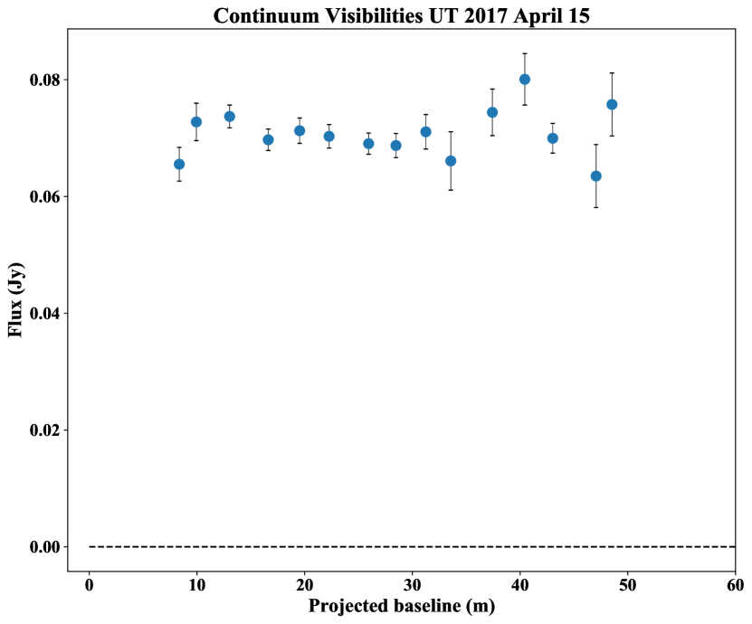
Figure 10: Visibility amplitude vs. projected baseline for continuum in ER61 on UT 2017 April 15.

Comet ER61 underwent a 2 mag outburst that started on April 3.9 and peaked near April 6.6 UT (Sekanina, 2017). The ER61 ACA observations were thus obtained 7.7–11.5 days after the onset of this major outburst. Taking into account the elapsed time between the outburst onset time and the ACA observations, the compact coma observed at 0.85 mm could be explained if the dust particles mainly contributing to the observed emission had velocities significantly less than 4 m s^-1. This population of slowly moving dusty material would correspond to large debris resulting from nucleus fragmentation, which was inefficiently accelerated by the gas pressure. The fast-moving, i.e. small particles, were observed in the optical. Opitom et al. (2019) collected dust brightness maps of comet ER61 at 710 nm on April 9 showing extended dust emission with $\sim$ 30 arcsec radius, that would correspond to projected dust velocities of $\sim$ 40 m s^-1. Maps of the dust color show a color gradient with the dust becoming bluer when further from the nucleus, consistent with the natural dust size sorting expected after an outburst, that is, smaller particles dominating the outer coma and larger particles the inner coma (Opitom et al., 2019).

The exceptional outburst of comet 17P/Holmes in 2007 October at r_H = 2.4 au was observed with the Plateau de Bure interferometer on two dates, 3.8 and 4.9 days after the outburst onset (Boissier et al., 2012). The 3 mm dust continuum emission was resolved by the $\sim$ 7000 km projected synthesized beam, but was more compact and 20% less intense on the latter date. The 17P data are best explained by the presence of two components: a slow-moving (7–9 m s^-1 for 1 mm particles), unresolved ‘core’ component, and a high-velocity component (50–100 m s^-1 for 1 mm particles) with a steep size distribution corresponding to the fast expanding shell observed in optical images (Boissier et al., 2012). The compact dust cloud observed in comet ER61 seems to be analogous to the core component of comet 17P, except that its thermal emission increased by a factor two between April 11 and 15, whereas it remained approximately constant in 17P. The non-detection of the fast expanding shell in comet ER61 can be explained by its residence time within the ACA beam, of about a day for particles at 50 m s^-1.

The measured flux densities $S_{\lambda}$ allow us to derive the mass of the core component around ER61’s nucleus, following:

$$S_{\lambda}=\frac{2kT_{\rm dust}M_{\rm core}k_{\lambda}}{\lambda^{2}\Delta^{2}}$$ (2)

where $T_{\rm dust}$ is the dust temperature (taken equal to the equilibrium temperature at the comet heliocentric distance, i.e. 259 K), and $k_{\lambda}$ is the dust opacity at the wavelength $\lambda$. The dust opacity depends on the dust size distribution and material optical properties. We used the opacity values computed by Boissier et al. (2012) at $\lambda$ = 0.8 mm for a size index of –3, a maximum size of 10 cm, and a dust porosity of 50%. For optical constants corresponding to astronomical (amorphous) silicates or silicate mixtures made of 20% amorphous silicates and 80% forsterite, mixed with water ice in various proportions, the derived opacities are in the range 2–4 $\times$ 10^-2 m² kg^-1. Taking the mean value, we derive dust masses of $\sim$ 5 $\times$ 10¹⁰ kg and 8 $\times$ 10¹⁰ kg for April 11 and 15, respectively. We did not consider the 15–30% possible nucleus contribution to the measured $S_{\lambda}$. The dust masses are five times smaller if we set the maximum size to 1 cm. For comparison, using the same assumptions about the dust properties, the core of 17P Holmes is found to be 3–5 times more massive. The derived dust mass is a lower limit to the total mass released during the outburst of ER61 and does not include that of the fragment which was observed near the comet several weeks after the outburst (Sekanina, 2017).

Meech et al. (2017) determined a nucleus radius r_N = 10 km, so our calculated dust mass on April 11 would constitute 0.0024% of the nucleus mass. This corresponds to a fragment with a 288 m radius and suggests that a major fragmentation event occurred. The outburst duration (defined as the temporal distance from the onset to the peak brightness) is 2.6 days (Sekanina, 2017); therefore, the production rate related to the outburst is 5 $\times$ 10¹⁰ kg / 2.6 days = 2.23 $\times$ 10⁵ kg s^-1. There is no constraint on the dust production rate for the quiescent activity of ER61 in the literature. Given that the water production rate was $\sim$3587 kg s^-1 and assuming a dust/gas ratio of unity, the dust release rate was 62 times higher (average over 2.6 days) than during quiescent activity.

The factor of two increase of the flux density between April 11 and 15 (actually 1.9 $\pm$ 0.3 when not considering the nucleus contribution to the flux density, 2.2 $\pm$ 0.4 when the nucleus contribution is considered) is puzzling. A possible explanation is that the core is optically thick. In this case, we would expect its brightness to vary linearly with the projected surface area of the core and with the square of the elapsed time since the outburst onset, assuming that its size varies linearly with time (case of spherical expansion at constant velocity). Under this assumption, a factor of 2.2 increase is expected, which is consistent with the data. However, if the core is optically thick, its physical size can then be estimated for the two dates and its expansion velocity can be derived. Applying the NEATM model described above, we derive a 19 km radius for April 11, and a 25 km radius for April 15. The assumption of an optically thick coma yields a coma expansion velocity of only 0.02 m s^-1, much below the escape velocity at the nucleus surface of about 5 m s^-1 for a 10 km radius nucleus. Hence, the dust coma observed with ACA was most likely optically thin. A possible explanation is then dust fragmentation, which increases the dust cross-section for the same mass of material. Besides the nucleus breakup, Sekanina (2017) suggested based on analysis of the light curves that the ejecta underwent fragmentation processes. Indeed, the extreme variability of the ER61 companion’s activity suggests that it progressively shedded debris until its full disintegration by the end of 2017 June (Sekanina, 2017).

Dust fragmentation is a highly complex process, and providing a comprehensive model of dust fragmentation in ER61 is beyond the scope of this work. However, we can comment on the residence time of particles in the ACA beam in this instance. As earlier noted, based on the dust velocity measured in 17P/Holmes with the Plateau de Bure interferometer, the dust velocity is 7–9 m s^-1 for 1 mm particles. For a velocity varying with particle size as a^-0.5, this results in velocities of 2.5 m s^-1 for 1 cm particles and 0.8 m s^-1 for 10 cm particles, giving residence times of 2.17 days, 7 days, and 22 days for sizes of 1 mm, 1 cm, and 10 cm particle radii, respectively. Inversely, if we impose that the residence time should be less than 11.5 d (the time between outburst onset and April 15) so that the same large-size material is present on both dates, we find a constraint that the particles should have a velocity less than 1.5 m s^-1. Sekanina (2017) estimated that the escape velocity of the detected companion was 0.9 m s^-1, consistent with our calculated values.

6 Conclusion

The powerful 12 m ALMA array has provided a window into the abundances and spatial distributions of volatiles in the inner coma with exceptional detail. Previous work with the main 12 m array has discerned parent from product species with high angular resolution maps of inner coma volatiles, revealed new insights into the origins of cometary HNC, probed the thermal physics of the inner coma, and detected the first parent volatiles in an interstellar comet (Cordiner et al., 2014, 2017a, 2017b, 2020; Bøgelund & Hogerheijde, 2017). However, the 12 m array is not always in the ideal configuration during a cometary apparition.

Due to the predetermined configuration schedule in any given observing cycle, the array can be in its more extended configurations during peak comet activity, where it resolves out extended flux and is blind to large-scale structure in the coma. Indeed, previous calculations have shown that the ACA is more sensitive to cometary flux than the 12 m array for configurations more extended than C43-4. However, this depends on the species lifetime, heliocentric and geocentric distance, as well as L_p (in the case of distributed sources). Still, the ACA is competitive with the 12 m array even in its most compact (C43-1) configuration. As an example, we consider a comet with Q(H₂O) = 1 $\times$ 10²⁹ s^-1 at r_H = $\Delta$ = 1 au, with T_kin = 70 K and a typical line width of 2 km s^-1. Using the ALMA Sensitivity Calculator, we find that in 3 hr of observing time the HCN (J = 4 – 3) transition could be securely detected (5$\sigma$) down to abundances of HCN/H₂O = 0.011% for the ACA, HCN/H₂O = 0.003% for the 12 m array in configuration C43-1, HCN/H₂O = 0.012% for C43-4, and HCN/H₂O = 0.024% for C43-5. Although these values are all consistent with strongly depleted abundances among measured comets, this highlights the increased sensitivity (by a factor of two for C43-5) of the ACA for studying coma chemistry compared to more extended 12 m configurations.

The work presented here demonstrates the power of the 7 m ACA for cometary observations, providing a valuable tool for probing larger scales in the coma, highly complementary to the 12 m array. Our measurements indicate that HCN production was predominantly from nucleus sources in ER61, whereas CS, H₂CO, and HNC were produced by distributed coma sources. CH₃OH may have also been associated with a distributed source, perhaps icy grains, although our measurements cannot rule out direct nucleus release. Parent scale lengths on the order of 2200 km for H₂CO and 3300 km for HNC are consistent with previous work, suggesting that both molecules are produced from photolysis or thermal degradation of polymers, dust grains, and/or the organic macromolecular material found by Rosetta at comet 67P/Churyumov–Gerasimenko (Capaccioni et al., 2015). A parent scale length of 2000 km for CS is consistent with distributed source production of CS in the extended coma from an unknown parent and cannot be fully explained by CS₂ photolysis in the inner coma. Continuum emission in ER61 is consistent with unresolved thermal emission from slowly moving outburst ejectas. Assuming a maximum dust size of 10 cm, we derive dust masses of $\sim$ 5 $\times$ $10^{10}$ kg and 8 $\times$ $10^{10}$ kg for April 11 and 15, respectively. The factor of two increase in flux density between April 11 and 15 may have been due to dust fragmentation in the optically thin coma.

Our observations between 7.7 – 11.5 days after ER61’s April outburst indicate that it is depleted in HCN and CO but consistent with the average for CS, HNC, CH₃OH, and H₂CO compared to abundances measured in its dynamical class. Our results show the wealth of information regarding molecular abundances, spatial distributions, mechanisms of molecular production, and coma temperatures that can be revealed in moderately bright comets such as ER61 with standalone ACA observations and highlight the important role that the ACA will play in future cometary studies.

Appendix A Effective Solar Pumping Rates

The ACA measurements presented here sampled emission from nucleocentric distances of $\sim$2000–24,000 km (the angular resolution of the longest ACA baseline to that of the ACA autocorrelation primary beam). As suggested by the divergence of the best-fit rotational and kinetic temperatures, non-LTE effects are important and must be accounted for at such large nucleocentric distances. Although rotational states in the inner coma (several hundred km from the nucleus) are thermalized by collisions, rotational populations at larger nucleocentric distances are governed by fluorescence equilibrium.

For a more complete treatment of the extended non-LTE coma sampled by our observations, fluorescence pumping by solar radiation must be considered, in which excited vibrational states pumped up by solar radiation decay through fluorescence, in turn further pumping the rotational levels in the ground vibrational state. We calculated effective solar pumping rates for CO, CS, CH₃OH, H₂CO, and HNC as in Zakharov et al. (2007) and Crovisier & Encrenaz (1983), and scaled them by the heliocentric distance of ER61 at the time of our observations. HCN pumping rates were adopted from Cordiner et al. (2019). We considered pumping by resonant fluorescence transitions (i.e., hot bands were excluded) for each species. We calculated pumping rates and Einstein-A’s using the HITRAN molecular database (Gordon et al., 2017) for CO, CS, CH₃OH, and H₂CO, and the GEISA molecular database (Jacquinet-Husson et al., 2016) for HNC. Rotational levels were mapped from HITRAN or GEISA to the LAMDA molecular database (Schöier et al., 2005) and the pumping rate for each level applied to our non-LTE radiative transfer models.

References

- A’Hearn et al. (1995) A’Hearn, M. F., Millis, R. L., Schleicher, D. G., Osip, D. J., & Birch, V. P. 1995, Icarus, 118, 223
- Altwegg et al. (2020) Altwegg, K., Balsiger, H., Hänni, N., et al. 2020, NatAs, 4, 533
- Biver (2015) Biver, N. 2015, Science Advances, 1, e1500863
- Biver et al. (1999) Biver, N., Bockelée-Morvan, D., Crovisier, J., et al. 1999, AJ, 118, 1850
- Bockelée-Morvan & Biver (2017) Bockelée-Morvan, D., & Biver, N. 2017, PTRSA, 375, 20160252, doi: 10.1098/rsta.2016.0252
- Bockelée-Morvan et al. (1994) Bockelée-Morvan, D., Crovisier, J., Colom, P., & Despois, D. 1994, A&A, 287, 647
- Bockelée-Morvan et al. (2004) Bockelée-Morvan, D., Crovisier, J., Mumma, M. J., & Weaver, H. A. 2004, in Comets II, ed. H. U. Keller & H. A. Weaver (University of Arizona Press), 391
- Bockelée-Morvan et al. (2000) Bockelée-Morvan, D., Lis, D. C., Wink, J. E., et al. 2000, A&A, 353, 1101
- Bøgelund & Hogerheijde (2017) Bøgelund, E. G., & Hogerheijde, M. R. 2017, A&A, 604, A131
- Boissier et al. (2007) Boissier, J., Bockelée-Morvan, D., Biver, N., et al. 2007, A&A, 475, 1131
- Boissier et al. (2012) Boissier, J., Bockelée-Morvan, D., Biver, N., et al. 2012, A&A, 542, A73, doi: 10.1051/0004-6361/201219001
- Boissier et al. (2011) Boissier, J., Groussin, O., Jorda, L., et al. 2011, A&A, 528, A54, doi: 10.1051/0004-6361/201016060
- Boissier et al. (2014) Boissier, J., Bockelée-Morvan, D., Biver, N., et al. 2014, Icarus, 228, 197
- Bonev et al. (2021) Bonev, B. P., Dello Russo, N., DiSanti, M. A., et al. 2021, PSJ, 2, 45
- Brinch & Hogerheijde (2010) Brinch, C., & Hogerheijde, M. R. 2010, A&A, 523, A25
- Calmonte et al. (2016) Calmonte, U., Altwegg, K., Balsiger, H., et al. 2016, MNRAS, 462, S253, doi: 10.1093/mnras/stw2601
- Capaccioni et al. (2015) Capaccioni, F., Coradini, A., Filacchione, G., et al. 2015, Science, 6220, aaa0628
- Cochran et al. (2012) Cochran, A. L., Barker, E. S., & Gray, C. L. 2012, Icarus, 218, 144
- Cordiner et al. (2014) Cordiner, M. A., Remijan, A. J., Boissier, J., et al. 2014, ApJL, 792, L2
- Cordiner et al. (2017a) Cordiner, M. A., Biver, N., Crovisier, J., et al. 2017a, ApJ, 837, 177
- Cordiner et al. (2017b) Cordiner, M. A., Boissier, J., Charnley, S. B., et al. 2017b, ApJ, 838, 147
- Cordiner et al. (2019) Cordiner, M. A., Palmer, M. Y., de Val-Borro, M., et al. 2019, ApJL, 870, L26
- Cordiner et al. (2020) Cordiner, M. A., Milam, S. N., Biver, N., et al. 2020, NatAs, doi: https://doi.org/10.1038/s41550-020-1087-2
- Cottin & Fray (2008) Cottin, H., & Fray, N. 2008, Space Science Reviews, 138, 179
- Crovisier et al. (2009) Crovisier, J., Biver, N., Bockelée-Morvan, D., & Colom, P. 2009, P&SS, 57, 1162
- Crovisier & Encrenaz (1983) Crovisier, J., & Encrenaz, T. 1983, A&A, 126, 170
- Dello Russo et al. (2016a) Dello Russo, N., Kawakita, H., Jr., V. R. J., & Weaver H., A. 2016a, Icarus, 278, 301
- Dello Russo et al. (2016a) Dello Russo, N., Kawakita, H., Vervack, R. J. J., & Weaver, H. A. 2016a, Icarus, 278, 301
- Drahus et al. (2012) Drahus, M., Jewitt, D., Guilbert-Lepoutre, A., Waniak, W., & Sievers, A. 2012, ApJ, 756, 80
- Feldman et al. (2004) Feldman, P. D., Cochran, A. L., & Combi, M. R. 2004, in Comets II, ed. H. U. Keller & H. A. Weaver (University of Arizona Press), 425
- Fray et al. (2006) Fray, N., Bénilan, Y., Biver, N., et al. 2006, Icarus, 184, 239
- Gomes et al. (2005) Gomes, R., Levison, H. F., Tsiganis, K., & Morbidelli, A. 2005, Nature, 435, 466
- Gordon et al. (2017) Gordon, I. E., Rothman, L. S., Hill, C., et al. 2017, JQSRT, 203, 3, doi: 10.1016/j.jqsrt.2017.06.038
- Harris (1998) Harris, A. W. 1998, Icarus, 131, 291, doi: 10.1006/icar.1997.5865
- Haser (1957) Haser, L. 1957, BSRSL, 43, 740
- Huebner & Mukherjee (2015) Huebner, W. F., & Mukherjee, J. 2015, P&SS, 106, 11, doi: 10.1016/j.pss.2014.11.022
- Irvine et al. (1998) Irvine, W. M., Bergin, E. A., Dickens, J. E., et al. 1998, Nature, 393, 547
- Jackson et al. (1986) Jackson, W. M., Butterworth, P. S., & Ballard, D. 1986, ApJ, 304, 515, doi: 10.1086/164185
- Jacquinet-Husson et al. (2016) Jacquinet-Husson, N., Armante, R., Scott, N. A., et al. 2016, JMoSp, 327, 31, doi: 10.1016/j.jms.2016.06.007
- Levison et al. (2011) Levison, H. F., Morbidelli, A., Tsiganis, K., Nesvorny, D., & Gomes, R. 2011, AJ, 142, 152
- Lis et al. (2008) Lis, D. C., Bockelée-Morvan, D., Boissier, J., et al. 2008, ApJ, 675, 931
- Lis et al. (2019) Lis, D. C., Bockelée-Morvan, D., Güsten, R., et al. 2019, A&A, 625, L5
- McMullin et al. (2007) McMullin, J. P., Waters, B., Schiebel, D., Young, W., & Golap, K. 2007, in Astronomical Data Analysis Software and Systems XVI ASP Conference Series, ed. R. A. Shaw, F. Hill, & D. J. Bell, Vol. 376 (San Francisco, CA: ASP), 127
- Meech et al. (2017) Meech, K. J., Schambeau, C. A., Sorli, K., et al. 2017, AJ, 153, 206, doi: 10.3847/1538-3881/aa63f2
- Meier et al. (1993) Meier, R., Eberhardt, P., Krankowsky, D., & Hodges, R. R. 1993, A&A, 277, 677
- Mifsud et al. (2021) Mifsud, D. V., KaÅuchová, Z., Herczku, P., et al. 2021, SSRv, 217, 14, doi: 10.1007/s11214-021-00792-0
- Milam et al. (2006) Milam, S. N., Remijan, A. J., Womack, M., et al. 2006, ApJ, 649, 1169
- Morbidelli et al. (2005) Morbidelli, A., Levison, H. F., Tsiganis, K., & Gomes, R. 2005, Nature, 435, 462
- Ootsubo et al. (2012) Ootsubo, T., Kawakita, H., Hamada, S., et al. 2012, ApJ, 752, 15
- Opitom et al. (2019) Opitom, C., Yang, B., Selman, F., & Reyes, C. 2019, A&A, 628, A128, doi: 10.1051/0004-6361/201833960
- Rabli & Flower (2010) Rabli, D., & Flower, D. R. 2010, MNRAS, 406, 95, doi: 10.1111/j.1365-2966.2010.16671.x
- Roth et al. (2021) Roth, N. X., Milam, S. N., Cordiner, M. A., et al. 2021, PSJ, 2, 55
- Saki et al. (2020) Saki, M., Gibb, E. L., Bonev, B., et al. 2020, AJ, 160, 184
- Saki et al. (2021) Saki, M., Gibb, E. L., Bonev, B. P., et al. 2021, AJ, 162, 165
- Schöier et al. (2005) Schöier, F. L., van der Tak, F. F. S., van Dishoeck, E. F., & Black, J. H. 2005, A&A, 432, 369, doi: 10.1051/0004-6361:20041729
- Sekanina (2017) Sekanina, Z. 2017, arXiv e-prints, arXiv:1712.03197. https://arxiv.org/abs/1712.03197
- Zakharov et al. (2007) Zakharov, V., Bockelée-Morvan, D., Biver, N., Crovisier, J., & Lecacheux, A. 2007, A&A, 473, 303, doi: 10.1051/0004-6361:20066715