Machine Learning Universal Bosonic Functionals

Abstract

The one-body reduced density matrix $\gamma$ plays a fundamental role in describing and predicting quantum features of bosonic systems, such as Bose-Einstein condensation. The recently proposed reduced density matrix functional theory for bosonic ground states establishes the existence of a universal functional $\mathcal{F}[\gamma]$ that recovers quantum correlations exactly. Based on a novel decomposition of $\gamma$, we have developed a method to design reliable approximations for such universal functionals: our results suggest that for translational invariant systems the constrained search approach of functional theories can be transformed into an unconstrained problem through a parametrization of an Euclidian space. This simplification of the search approach allows us to use standard machine-learning methods to perform a quite efficient computation of both $\mathcal{F}[\gamma]$ and its functional derivative. For the Bose-Hubbard model, we present a comparison between our approach and Quantum Monte Carlo.

In 1964 Hohenberg and Kohn proved the existence of a universal functional $\mathcal{F}[\rho]$ of the particle density $\rho$, that captures the exact electronic contribution to the ground-state energy of a system of interacting electrons Hohenberg and Kohn (1964). Due to a remarkable balance of accuracy and computational cost, first principle modeling of electronic systems based on the respective Density Functional Theory (DFT) is nowadays a well established daily practice, with great impact in material science, quantum chemistry or condensed matter Jones (2015). For bosonic systems, however, a fully first-principle description has been elusive. This is due in part to the unsuitability of the particle density to describe fundamental bosonic features as orbital occupations, mode entanglement, or non-diagonal order, which are important for predicting and describing bosonic condensation. As a result, the theoretical treatment of interacting bosonic systems mainly relies on exact diagonalization techniques, which are restricted to few tens of orbitals Cazalilla et al. (2011); Chatterjee et al. (2020); González-Cuadra et al. (2018), or mean-field theories that are particularly suitable for dilute ultracold gases Fisher et al. (1989); Pitaevskii and Stringari (2003); Dalfovo et al. (1999). Quantum Monte Carlo (QMC) is known to be a powerful family of techniques for computing ground-state properties but is still restricted due to the fermion sign problem. While bosonic systems do not suffer such a sign problem, QMC cannot be applied to, e.g., frustrated quantum spin systems Gubernatis et al. (2016). Nowadays, a renewed interest in the ab-initio description of many-body systems has been motivated by the successful application of artificial neural networks to both fermionic and bosonic problems Saito (2017); Choo et al. (2018).

Since the parameters of correlated bosonic systems (ultracold gases, in particular) can be tuned with a high degree of control, they are powerful platforms to study a wide range of model Hamiltonians, ranging from Hubbard models to bosonic antiferromagnets Bloch et al. (2008); Chin et al. (2010). They have also become an active research field in the context of quantum simulations Bloch (2005); Gross and Bloch (2017); Schäfer et al. (2020), and even quantum foundations Schmied et al. (2016); Fadel et al. (2018); Kunkel et al. (2018); Lange et al. (2018). Such need to describe quantum correlations of bosonic systems efficiently has motivated quite recently to put forward a novel physical theory for interacting bosonic systems Benavides-Riveros et al. (2020); Liebert and Schilling (2021). Based on a generalization of the Hohenberg-Kohn theorem Gilbert (1975); Pernal and Giesbertz (2016), this reduced density matrix functional theory (RDMFT) for bosons establishes the existence of a universal functional $\mathcal{F}_{W}[\gamma]$ of the one-body reduced density matrix (1RDM): $\gamma\equiv N\mbox{Tr}_{N-1}[\Gamma]$, obtained from the $N$-boson density operator $\Gamma$ by integrating out all except one boson, and the two-particle interaction $\hat{W}$. Since the 1RDM is the natural variable of the theory, RDMFT is particularly well-suited for the accurate description of Bose-Einstein condensates (BEC), strongly correlated bosonic systems, or fragmented BEC Sakmann et al. (2008); Bulgac and Jin (2017). Furthermore, the information contained in the spectra of the 1RDM can also be sufficient to investigate multipartite quantum correlations in those systems Aloy et al. (2021); Walter et al. (2013); Sawicki et al. (2014, 2012); Yu et al. (2021).

Although RDMFT holds the promise of abandoning the complex $N$-particle wave function as the central object, it does not trivialize the ground-state problem. In fact, the fundamental challenge is to provide reliable approximations to the universal interaction functional $\mathcal{F}_{W}[\gamma]$. Yet, while the Hohenberg-Kohn-type fundational theorem of RDMFT shows the existence of a universal functional, it does not give any indication of its concrete form. For DFT, the solution to this problem is given in the form of large classes of approximate functionals, hierarchically organized in the so-called Jacob’s ladder. In recent years, the number of such approximation has significantly increased thanks to machine learning Kalita et al. (2021); Brockherde et al. (2017); Schmidt et al. (2019a); Li et al. (2021); Margraf and Reuter (2021); Moreno et al. (2020) and reduced density matrices Gibney et al. (2021) approaches.

Our work succeeds in providing a strategy on computing approximations for $\mathcal{F}_{W}[\gamma]$. In this paper we (i) provide an efficient method to capture the essential features of universal functionals for boson lattices, (ii) show how the constrained search approach associated with it can be simplified in the form of an unconstrained problem, and (iii) implement this approach in a standard machine-learning library to compute $\mathcal{F}_{W}[\gamma]$, its derivative, and the ground-state energy. We shall for simplicity describe our method for the Bose-Hubbard model, but the same results apply to any type of interactions for systems with translational symmetry.

Universal bosonic functionals.— In this work we consider Hamiltonians of the form

$$\hat{H}_{W}(\hat{h})\equiv\hat{h}+\hat{W},$$ (1)

with a one-particle term $\hat{h}=\hat{t}+\hat{v}$, containing the kinetic energy and the external potential terms, and the two-particle interaction $\hat{W}$. The ground-state energy and 1RDM follow for any choice of the one-particle Hamiltonian $h$ from the minimization of the total energy functional $\mathcal{E}_{h}[\gamma]=\mbox{Tr}[h\gamma]+\mathcal{F}_{W}[\gamma]$. The functional $\mathcal{F}_{W}[\gamma]$ is universal in the sense that it depends only on the fixed interparticle interaction $W$, and not on the one-particle Hamiltonian $\hat{h}$. Hence, determining the functional $\mathcal{F}_{W}[\gamma]$ would in principle entail the simultaneous solution of the universal correlation part of the ground state problem for any Hamiltonian $H_{W}(h)$. By writing the ground-state energy as $E(h)\equiv\min_{\Gamma}\mbox{Tr}_{N}[H_{W}(h)\Gamma]$, and using the fact that the expectation value of $h$ is determined by $\gamma$, one can replace the functional $\mathcal{F}_{W}[\gamma]$ by the well-known constrained search approach Levy (1979):

$$\mathcal{F}_{W}[\gamma]=\min_{\Gamma\mapsto\gamma}\mbox{Tr}_{N}[W\Gamma]\,,$$ (2)

where $\Gamma\mapsto\gamma$ indicates that the minimization is carried out over all $\Gamma$ whose 1RDM is $\gamma$. The main challenge of this approach is that the set of $\Gamma$ such that $\Gamma\mapsto\gamma$ is in general extremely complex to characterize, and so far only partial results are known for quasi-extremal, two-particle or translational invariant fermionic systems Schilling et al. (2020); Löwdin and Shull (1956); Schilling and Schilling (2019); Giesbertz (2020); Fadel et al. (2020). Even in the extremely popular DFT, the constrained search over many-body wave functions integrating to the same electronic density (i.e., $\Psi\rightarrow\rho$) is rarely explicitly carried out Mori-Sánchez and Cohen (2018).

To shed some light on the problem let us represent $\gamma$, the 1RDM of a $N$-boson real wave function $|\Psi\rangle$, with respect to a set of creation and annihilation operators

$$\gamma_{ij}=\mbox{$\langle\Psi|$}\hat{b}^{\dagger}_{i}\hat{b}_{j}\mbox{$|\Psi\rangle$}\,,$$ (3)

and assume that the dimension of the one-particle Hilbert space is $M$. Let us also define $M$ ($N-1$)-particle wave functions $\mbox{$|\Phi_{j}\rangle$}\equiv\hat{b}_{j}\mbox{$|\Psi\rangle$}$, which satisfy by definition the condition

$$\mbox{$\langle\Phi_{i}|$}\Phi_{j}\rangle=\gamma_{ij}\,.$$ (4)

The meaning of these non-normalized wave functions is clear: while their magnitude equals the diagonal entries of $\gamma$ (i.e., $\mbox{$\langle\Phi_{j}|$}\Phi_{j}\rangle=\gamma_{jj}$), the angles they form correspond to the non-diagonal entries of $\gamma$. Indeed, since $\mbox{$\langle\Phi_{i}|$}\Phi_{j}\rangle=||\Phi_{i}||||\Phi_{j}||\cos(\theta_{ij})=\sqrt{\gamma_{ii}\gamma_{jj}}\cos(\theta_{ij})$ we have

$$\cos(\theta_{ij})=\frac{\gamma_{ij}}{\sqrt{\gamma_{ii}\gamma_{jj}}}\,.$$ (5)

The bound of the non-diagonal entries: $|\gamma_{ij}|^{2}\leq\gamma_{ii}\gamma_{jj}$, is the Cauchy-Schwarz inequality for operators, and known to be a representability condition for $\gamma$ Giesbertz and Ruggenthaler (2019). The condition $\sum_{j}\hat{b}_{j}^{\dagger}\mbox{$|\Phi_{j}\rangle$}=N\mbox{$|\Psi\rangle$}$ suggests that the minimizer of the minimization (2) can be written as a set of $M$ vectors in the Hilbert space $\mathcal{H}_{N-1}$ of $N-1$ particles, such that their angles and magnitudes are determined by Eq. (4) (see Fig. 1). We now exploit this first insight to explicitly carry out the constrained search approach and find the universal functional of the Bose-Hubbard model, a workhorse in the context of ultracold bosonic atoms Jaksch et al. (1998).

Figure 1: Representation of 3 wave functions in the Hilbert space of $N-1$ particles giving place to a 1RDM $\gamma$. While the magnitude of the vectors is $||\Phi_{i}||^{2}=\gamma_{ii}$, the angles they form satisfy $\mbox{$\langle\Phi_{i}|$}\Phi_{j}\rangle=\sqrt{\gamma_{ii}\gamma_{jj}}\cos(\theta_{ij})$.

Bose-Hubbard model.— The Hamiltonian of the Bose-Hubbard model reads:

$$H=-t\sum_{\langle ij\rangle}\hat{b}_{i}^{\dagger}\hat{b}_{j}+\frac{U}{2}\!\sum^{M}_{j=1}\!\hat{n}_{j}(\hat{n}_{j}-1)\,,$$ (6)

where the operator $\hat{b}^{\dagger}_{j}$ ($\hat{b}_{j}$) create (annihilate) a boson on site $j$, and $\hat{n}_{j}$ is the corresponding number operator. The first term in Eq. (6) describes the hopping between two sites while the second one is the interacting term $\hat{W}=\frac{U}{2}\sum_{j}\!\hat{n}_{j}(\hat{n}_{j}-1)$. Since the problem is determined by $N$ spinless bosons and $M$ sites, we write for the functional $\mathcal{F}_{N,M}[\gamma]$. For a given $\gamma$ let us take the minimizer of the functional (2) and call it $\mbox{$|\Psi_{\gamma}\rangle$}\in\mathcal{H}_{N}$, the $N$-particle Hilbert space. Using the prescription discussed above let us define $M$ ($N-1$)-particle wave functions $\mbox{$|\Phi_{\gamma,j}\rangle$}\equiv\hat{b}_{j}\mbox{$|\Psi_{\gamma}\rangle$}\in\mathcal{H}_{N-1}$, which satisfy by definition the condition (4). Due to the translational invariance of the Bose-Hubbard Hamiltonian (6), these wave functions are all normalized to the filling factor, namely, $\mbox{$\langle\Phi_{\gamma,i}|$}\Phi_{\gamma,i}\rangle=N/M$. The functional is given by $\mathcal{F}_{N,M}[\gamma]=\sum_{i}\mbox{$\langle\Phi_{\gamma,i}|$}\hat{n}_{i}\mbox{$|\Phi_{\gamma,i}\rangle$}$, using $\hat{n}_{i}(\hat{n}_{i}-1)=\hat{b}^{\dagger}_{i}\hat{n}_{i}\hat{b}_{i}$. As shown in the Appendix B, any rotation of the states $|\Phi_{\gamma,i}\rangle$ in the subspace spanned by themselves: $\mathcal{G}_{\gamma}={\rm span}\{\mbox{$|\Phi_{\gamma,1}\rangle$},\dots,\mbox{$|\Phi_{\gamma,M}\rangle$}\}$, will give an energy greater or equal than the energy $\mathcal{F}_{N,M}[\gamma]$. As a consequence, we rewrite the constrained search approach in Eq. (2) as

$$\mathcal{F}_{N,M}[\gamma]=\min_{\{\Phi_{i}\}\in\mathcal{G}_{\gamma}}\sum_{i}\mbox{$\langle\Phi_{i}|$}\hat{n}_{i}\mbox{$|\Phi_{i}\rangle$}\,,$$ (7)

subject to $\mbox{$\langle\Phi_{i}|$}\Phi_{i}\rangle=N/M$ and $\mbox{$\langle\Phi_{i}|$}\Phi_{j}\rangle=\gamma_{ij}$. This indicates that the constraint in Eq. (2) can be transferred to the subspace $\mathcal{G}_{\gamma}$. As we will see below, this result leads to a quite efficient optimization problem for the functional.

Exact functional of the dimer.— As a first illustration of this novel approach let us take the simple case of the Bose-Hubbard dimer with two particles ($N=M=2$). The states of the Hilbert space can be written as two occupations: $|n_{L},n_{R}\rangle$. For the 1-boson Hilbert space we choose as a basis: $\{\mbox{$|1,0\rangle$},\mbox{$|0,1\rangle$}\}$. We are interested in the minimum of $\mbox{$\langle\Phi_{L}|$}\hat{n}_{L}\mbox{$|\Phi_{L}\rangle$}+\mbox{$\langle\Phi_{R}|$}\hat{n}_{R}\mbox{$|\Phi_{R}\rangle$}$, such that $\mbox{$\langle\Phi_{L}|$}\Phi_{R}\rangle=\gamma_{LR}\equiv\cos(\theta)$. We write these two wave functions as $\mbox{$|\Phi_{L}\rangle$}=\sin(\theta_{L})\mbox{$|1,0\rangle$}+\cos(\theta_{L})\mbox{$|0,1\rangle$}$ and $\mbox{$|\Phi_{R}\rangle$}=\cos(\theta_{R})\mbox{$|1,0\rangle$}+\sin(\theta_{R})\mbox{$|0,1\rangle$}$. As a result of the corresponding minimization (7), the three angles are related: $\theta_{L}=\theta_{R}=(\pi/2-\theta)/2$, and the universal functional equals to:

$$\mathcal{F}_{2,2}(\theta)=2\sin^{2}\left(\frac{\pi}{4}-\frac{\theta}{2}\right)=1-\sin(\theta)\,,$$ (8)

which is one of the few analytical results for a universal functional that can be found in the literature Cohen and Mori-Sánchez (2016); Töws and Pastor (2011).

Machine learning.— Despite the spectacular rise of machine learning in the study of quantum many-body systems, no implementation is known so far for the theory of reduced density matrices Carleo et al. (2019); Carrasquilla (2020). One of the reasons for this lack of progress is the large amount of constraints swarming in functional theories. We now discuss how our findings will facilitate learning the universal functional of bosonic systems. Notice that a more appealing way of writing the functional in Eq. (7) is the following: Let us choose a basis for the vector space $\mathcal{G}_{\gamma}$, say: $\{\mbox{$|\mathbf{m}\rangle$}\in\mathcal{H}_{N-1}\}$. A set of wave functions of the sort needed in the minimization (7) can now be written as $\mbox{$|\Phi_{j}\rangle$}=\sum d_{j\mathbf{m}}\mbox{$|\mathbf{m}\rangle$}$. The condition of Eq. (4) reads: $\mathbf{d}\mathbf{d}^{\dagger}=\gamma$, where we have defined the matrix: $[\mathbf{d}]_{j\mathbf{m}}=d_{j\mathbf{m}}$. Using the singular value decomposition for such a matrix we have $\mathbf{d}=\mathbf{U}\mathbf{\Sigma}\mathbf{V}^{\dagger}$, with $\mathbf{U}$ and $\mathbf{V}$ $M\times M$ unitary matrices. Since $\mathbf{\Sigma}\mathbf{\Sigma}^{\dagger}=\mathbf{U}^{\dagger}\gamma\mathbf{U}$, it is now clear that the spectral decomposition of $\gamma$ equals to $\mathbf{\Sigma}\mathbf{\Sigma}^{T}$. As a consequence, we obtain $[\mathbf{\Sigma}]_{\alpha\alpha}=\sqrt{n_{\alpha}}$, where $\{n_{\alpha}\}$ are the eigenvalues of $\gamma$. Collecting these results we obtain that the exact universal functional (7) can be explicitly written in terms of the eigenvalues and the eigenvectors of $\gamma$ (contained in the matrix $\mathbf{U}$):

$$\mathcal{F}_{W}[\gamma]=\sum_{\alpha\beta}\sqrt{n_{\alpha}n_{\beta}}\Delta_{\alpha\beta}(\mathbf{U},\mathbf{V})\,,$$ (9)

where $\Delta_{\alpha\beta}(\mathbf{U},\mathbf{V})=\sum_{i,\mathbf{mm^{\prime}}}u^{*}_{i\alpha}u_{i\beta}v_{\mathbf{m}\alpha}^{*}v_{\mathbf{m^{\prime}}\beta}\mbox{$\langle\mathbf{m}^{\prime}|$}\hat{n}_{i}\mbox{$|\mathbf{m}\rangle$}$. The concrete form of the functional presented in Eq. (9) is striking: for fermionic density-matrix-functional theory, the square root of the occupation numbers in Eq. (9) is known to be the optimal choice for Ansätze of the form $n_{i}^{\alpha}n_{j}^{1-\alpha}$, compatible with the integral relation between the one- and two-body reduced density matrices Müller (1984); Buijse and Baerends (2002); Frank et al. (2007); Benavides-Riveros and Marques (2018), even for systems out of equilibirum Benavides-Riveros and Marques (2019). As we can see, the only freedom in the functional (9) is the matrix $\mathbf{V}$, which is, unlike $\mathbf{U}$ and $n_{\alpha}$, not fixed by $\gamma$. We use this degree of freedom to introduce a standard optimization problem on a connected manifold $\mathcal{M}$:

$$\mathcal{F}_{N,M}[\gamma]=\min_{\mathbf{V}\in\mathcal{M}}\sum_{\alpha\beta}\sqrt{n_{\alpha}n_{\beta}}\Delta_{\alpha\beta}(\mathbf{U}_{\gamma},\mathbf{V})\,,$$ (10)

where we have included a sub-index in $\mathbf{U}_{\gamma}$ to remember that such a matrix is defined by $\gamma$. Notice that the manifold $\mathcal{M}$ is essentially the set of special orthogonal matrices of dimension $M$, which generates the space $\mathcal{G}_{\gamma}$. Although the definition of such a space is far from trivial (and we will leave this question open for future research), it is possible to establish some elementary facts. For instance, in the strongly correlation regime $U/t\gg 1$ with integer filling factor $\alpha=N/M$, $\mathcal{G}_{\gamma}={\rm span}\{b_{i}\mbox{$|\alpha,...,\alpha\rangle$}\}$.

To make further progress on our problem, notice that optimization problems of the form $\min_{x\in\mathcal{M}}f(x)$ over a connected manifold $\mathcal{M}$ can be transformed into an unconstrained one of the form $\min_{y\in\mathbb{R}^{n}}f(\phi(y))$ by lifting the function $f$ to the current tangent space $T_{x}\mathcal{M}$ Lezcano-Casado (2019); Siegel (2020). The map $\phi:\mathbb{R}^{n}\rightarrow\mathcal{M}$ is called a trivialization map Lezcano-Casado (2019). By letting the minimization in Eq. (10) to run over the set of special orthogonal matrices in dimension $M$, the relevant minimization space turns out to be an Euclidian space $\mathbb{R}^{M}$. As a result, finding the universal functional of RDMFT presents itself as an unconstrained minimization problem. This is the crucial and last finding of our work, as it finally allows us to compute the universal bosonic functional by solving the problem directly over the set of orthonormal matrices.

Modern machine learning frameworks like pytorch Paszke et al. (2017) provide fast and rather efficient ways of performing optimizations on connected manifolds of the type we consider here. For the results we will present below, we have implemented the constrained minimization (10) in pytorch with the constrained minimization toolkit GeoTorch Geo . As a first step we implemented an minimization procedure where for each 1RDM the matrix $\mathbf{V}$ in Eq. (10) is optimized to produce the universal functional. As a second step we trained a neural network as the universal bosonic functional (see below).

Results.— In Fig. 6 we present the results for the Bose-Hubbard model (6) for $M$ sites and ($\alpha M$) bosons, for $M=2,4,6$ and $\alpha=1,2$. For this example, we have considered $\gamma$ of the form $\gamma_{ii}=\alpha$ and $\gamma_{ij}=\alpha\eta$, for $i\neq j$ with $0\leq\eta\leq 1$ (this choice ensures the positive semidefiniteness of $\gamma$). The systems are fully condensated when $\eta=1$ (i.e., an occupation number is macroscopically populated). For comparison, all functionals have been normalized to $0$ in the lower point (i.e., $\eta=0$) and to 1 in the upper point ($\eta=1$). The exact known results for $M=2$ in Eq. (8) are verified in our calculations. Furthermore, we observe the existence of the Bose-Einstein force discovered in Benavides-Riveros et al. (2020), extended in Liebert and Schilling (2021) and proved in Maciażek (2021), namely, the divergence of the gradient $\partial_{\eta}\mathcal{F}_{N,M}(\eta)\rightarrow(N-N_{\rm BEC})^{\zeta}$, with $\zeta<0$, when approaching to the condensation point (i.e., $\eta\rightarrow 1$). The striking similarities of the functionals $\mathcal{F}_{M,M}[\gamma]$ and $\mathcal{F}_{2M,M}[\gamma]$ suggests the existence of a universal functional independent of $\alpha$, up to appropriate normalizations.

Figure 2: Universal functionals $\mathcal{F}_{M,M}[\gamma]$ and $\mathcal{F}_{2M,M}[\gamma]$ for the $M$-site 1D Bose-Hubbard model with filling factor $\alpha=1,2$, for $M=2,4,6$ sites (see text). The functional corresponds to all 1RDM with $\gamma_{ii}=\alpha=N/M$ and $\gamma_{ij}=N\eta/M$ for $i\neq j$. All functionals are convex, as expected. For easy comparison, all functionals have been normalized to 0 in the lower point ($\eta=0$) and to 1 in the upper point ($\eta=1$).

In functional theories the knowledge of the functional’s form is as important as the knowledge of its derivative, as both are needed for a ground state calculation. To perform the derivative of the functional we trained a neural network to output the matrix $\mathbf{V}$ using the degrees of freedom of our 1RDM as input. This has multiple advantages. First, once the functional is trained for given particle and site numbers, it can be evaluated for any $\gamma$. Secondly, the automatic differentiation allows an exact evaluation of the gradient $\nabla_{\gamma}\mathcal{F}_{N,M}[\gamma]$ without further work. For the Bose-Hubbard dimer it was sufficient to use the diagonal terms $\eta=\gamma_{i(i+1)}$ and its square as inputs. The calculation was structured as follows:

$$\text{FCNN}_{N,M,\theta}(\eta,\eta^{2},\mathbf{US})\rightarrow\mathbf{V}\rightarrow\mathcal{F}_{N,M,\theta}\left[\gamma\right].$$ (11)

Here $\text{FCNN}_{N,M,\theta}$ is a fully connected network for $N$ particles and $M$ sites with the parameters $\theta$ and

$$\mathbf{US}=\mathbf{U}\times\begin{pmatrix}n_{0}&0&\cdots&0\\ 0&n_{1}&\cdots&0\\ \vdots&\vdots&\ddots&\vdots\\ 0&0&0&n_{M}\\ \end{pmatrix}$$ (12)

calculated from the eigenvectors $\mathbf{U}$ and eigenvalues $n_{i}$ of $\gamma$. During training we minimize the functional $\mathcal{F}_{N,M,\theta}\left[\gamma\right]$ for a set of $\gamma$ in parallel. The networks used 2 hidden layers, ELU-activation functions Clevert et al. (2015) and the output of the last layer was used to create an orthogonal matrix through a matrix exponential. The network for the dimer was trained on the set $\eta\in(0.005,0.001,\dots,0.995)$. When evaluating on the set $(0.0025,0.0075,\dots,0.9925)$ the maximum absolute error is smaller than $10^{-15}$. The network for $N=4$, $M=4$ was trained on the same set. Remarkably, as shown in Fig. 3, for the Bose-Hubbard dimer (for which we can compare to exact results) the derivatives provided by the neural network only deviate by $\sim 10^{-13}$ from the exact results.

Figure 3: Comparison between the gradient of the functional for the Bose-Hubbard dimer computed with the neural network and the exact analytical results as a function of $1-\eta$ (see text). Notice the log-log scale.

We demonstrate now that our approach allows us to compute the ground-state energy and 1RDM for a large system. Notice first that for a fixed filling factor $\alpha=N/M$, the energy of the ground state of the Bose-Hubbard model (6) can be computed as the minimum of the energy functional $\mathcal{E}_{N,M}[\gamma]=-2t\sum_{i}\gamma_{i(i+1)}+\mathcal{F}_{N,M}[\gamma]$. By performing the minimization $\nabla_{\gamma}\mathcal{E}_{N,M}[\gamma]=0$ on the domain of positive semidefinite matrices, it is then possible to compute the ground-state energy of the system. To generate the functional in that domain, we have optimized the ansatz $\gamma_{ij}=\eta^{\kappa}\alpha$ ($0\leq\eta\leq 1$) with $2\leq\kappa\leq 8$, for $|j-i|>1$, with $\eta=\gamma_{i(i+1)}$. This is motivated by the fact that when $U/t\gg 0$, $\gamma_{ij}\approx 0$, $\forall i>j$, and when $U/t\ll 1$ $\gamma_{ij}\approx\alpha$, $\forall ij$. Following this prescription we have computed the ground-state energy for the 40-site Bose-Hubbard model with 40 bosons. The dimension of the corresponding Hilbert spaces, being of the order of $5.3\times 10^{22}$, is out of reach for exact diagonalization and prohibits performing the exact constrained search approach. To solve this problem we have (i) ansatzen the space $\mathcal{G}_{\gamma}$, the subspace generated by the kets $\mbox{$|\Phi_{i}\rangle$}=\hat{b}_{i}\mbox{$|\Psi\rangle$}$, by choosing $\mbox{$|\Psi\rangle$}=\mbox{$|1,...,1\rangle$}$ (RDMFT1), and (ii) used the exact functional of the dimer (8), appropriately rescaled (RDMFT2). The energy predictions of our machine-learning functionals are quite remarkable, given the subspaces we have chosen. Indeed, the results presented in Fig. 4 indicate that the predicted RDMFT results are in good agreement with the QMC energies: the errors around $U/t=4$ are only due to the approximation of the space $\mathcal{G}_{\gamma}$. In order to check the quality of the approximate functionals more, we have also plotted the relative error in the last panel. We observe that this error is below 8% and practically zero for large and weak interaction. In addition, notice that our implementation is able to approximate the whole range of energies, not only the weakly (the sector easily described by Bogoliubov methods) or the strongly correlation regimens.

Figure 4: Ground-state energy of the $40$-site 1D Bose-Hubbard model with 40 bosons. In Fig. (a) the energy is plotted as a function of the relative strength $U/t$. In blue the results computed using the functional (10) (RDMFT1) and the ansatz $\mbox{$|\Phi_{i}\rangle$}=b_{i}\mbox{$|1,...,1\rangle$}$. In black we use as an ansatz for the functional the exact expression of the dimer appropriately rescaled (RDMFT2). In red the results computed with QMC. In the subfigure the functionals $\mathcal{F}_{N,N}(\eta)$ are plotted as a function of $\eta$, the nearest-neighbor off-diagonal value of the 1RDM. In Fig. (b) the relative errors $\Delta/E_{QMC}$, where $\Delta=E_{RDMFT2}-E_{QMC}$ are plotted as a function of U/t.

Conclusion.— In conclusion, we have demonstrated the viability of approximating universal bosonic functionals in a quite efficient way. The main ingredient of the computation is a simplification of the constrained search approach that we have introduced in this work based on the Schmidt decomposition of the wave function. This formulation of reduced density matrix functional theory (RDMFT) speeds up the design of reliable approximations for the universal functionals for systems with translational symmetry. The quality of the numerical results obtained in this work highlights the potential of RDMFT to become a competitive tool for computing properties of bosonic ground states with large dimensional Hilbert spaces. Strikingly, since RDMFT takes into account the whole range of bosonic correlations, and does not present dimensional or sign problems, it offers a range of new possibilities. For instance, frustrated bosonic systems can be studied in a direct manner Wang et al. (2009). Bosonic systems with impurities, composites of ultra-cold atoms, or even superconducting systems Hunter et al. (2020); Schmidt et al. (2019b, c); Alon et al. (2005) can also potentially be addressed within this framework. As an outlook of this work, we leave open a new line of research based on extending our findings to systems with internal degrees of freedom, finite temperatures, or broken symmetries. We also expect that previous works in the context of two-body reduced density matrix Mazziotti and Herschbach (1999); Gidofalvi and Mazziotti (2004) will also benefit from our approach.

All codes to reproduce, examine and improve our proposed analysis will be made freely available online upon publication.

Appendix A The $\gamma$-representability problem

An important problem in the theory of reduced density matrices for indistinguishable particles is the so-called $N$-representability problem, namely, which conditions should $\gamma$, the one-body reduced density matrix (1RDM), satisfy in order to belong to at least one wave function in $\mathcal{H}_{N}$, the Hilbert space of $N$ particles (fermions or bosons). To understand the problem, let us consider for a given wave function $\mbox{$|\Psi\rangle$}\in\mathcal{H}_{N}$ the corresponding 1RDM as:

$$\gamma^{\Psi}_{ij}=\mbox{$\langle\Psi|$}f^{\dagger}_{i}f_{j}\mbox{$|\Psi\rangle$}\,.$$ (13)

We have introduced a one-particle basis set $\mbox{$|f_{i}\rangle$}=f^{\dagger}_{i}\mbox{$|0\rangle$}$ that determines the corresponding set of creation and anhilitation operators. The matrix $\gamma$ has the following properties: (a) it satisfies the trace condition: $\sum_{i}\gamma^{\Psi}_{ii}=N$, (b) it is hermitian, and (c) it is positive semidefinite (i.e., its eigenvalues are non-negative). For fermions the Pauli exclusion principle imposes another constraint: $\gamma\leq 1$ Lieb and Seiringer (2009), and the generalized Pauli principle imposes even stronger constraints on the eigenvalues Klyachko (2006); Reuvers (2021). Another less explored problem is the following: what is the set of wave functions giving place to the same 1RDM, namely, what is the set of wave functions

$$\mathcal{S}_{\gamma}=\{\mbox{$|\Psi\rangle$}\in\mathcal{H}_{N}:\gamma_{ij}=\mbox{$\langle\Psi|$}f^{\dagger}_{i}f_{j}\mbox{$|\Psi\rangle$}\}\,$$ (14)

in the Hilbert space $\mathcal{H}_{N}$? The characterization of this set is of crucial importance for the ground state problem as seen from the point of view of reduced density matrix functional theory (RDMFT) Pernal and Giesbertz (2016). Indeed, it allows us to find the universal functional of a two-particle interaction $W$ defined as:

$$\mathcal{F}_{W}[\gamma]\equiv\min_{\Psi\in\mathcal{S}_{\gamma}}\mbox{$\langle\Psi|$}W\mbox{$|\Psi\rangle$}\,.$$ (15)

As a consequence of this construction, the ground state of a system of indistinguishable particles driven by a Hamiltonian $H(h)$ could be computed in a quite simple way by resorting only to the set of 1RDMs Levy (1979):

$$E_{0}=\min_{\Psi\in\mathcal{H}_{N}}\mbox{$\langle\Psi|$}H\mbox{$|\Psi\rangle$}=\min_{\gamma}\min_{\Psi\in\mathcal{S}_{\gamma}}\mbox{$\langle\Psi|$}H\mbox{$|\Psi\rangle$}=\min_{\gamma}\{\mbox{Tr}[h\gamma]+\min_{\Psi\in\mathcal{S}_{\gamma}}\mbox{$\langle\Psi|$}W\mbox{$|\Psi\rangle$}\}\,,=\min_{\gamma}\{\mbox{Tr}[h\gamma]+\mathcal{F}_{W}[\gamma]\}\,,$$ (16)

where $h$ contains all the 1-particle contributions to the full Hamiltonian $H(h)=h+W$.

Appendix B The Bose-Hubbard Hamiltonian

For clarity, we will work out the Bose-Hubbard model, but the results can be generalized for systems with translational symmetry. The Hamiltonian of the problem is given by:

$$H=-t\sum_{i}\left(b^{\dagger}_{i}b_{i+1}+\rm{h.c.}\right)+\frac{U}{2}\sum_{i}\hat{n}_{i}(\hat{n}_{i}-1)\,.$$ (17)

The two-particle interaction is $W=\frac{U}{2}\sum_{i}\hat{n}_{i}(\hat{n}_{i}-1)$ and the 1-particle Hamiltonian is $h=-t\sum_{i}(b^{\dagger}_{i}b_{i+1}+{\rm h.c.})$. We fix $N$ and $M$, the number of particles and the number of sites. The filling factor is defined by $\alpha=N/M$. Notice that the Hamiltonian is translational invariant. We further choose periodic boundary conditions.

B.1 Ground-state problem with reduced density matrices

The ground-state energy satisfies by definition: $E_{0}=\min_{\Psi\in\mathcal{H}_{N}}\mbox{$\langle\Psi|$}H\mbox{$|\Psi\rangle$}$. For a given wave function $|\Psi\rangle$ the expected value of the corresponding Hamiltonian reads:

$$\mbox{$\langle\Psi|$}H\mbox{$|\Psi\rangle$}=-t\sum_{i}\left(\gamma^{\Psi}_{i(i+1)}+c.c.\right)+\mbox{$\langle\Psi|$}W\mbox{$|\Psi\rangle$}.$$ (18)

Yet, since the Hamiltonian (17) is translational invariant, we have in general: $\gamma^{\Psi}_{ij}=\gamma^{\Psi}_{(i+m)(j+m)}$, for $m\geq 0$.

As a result, the ground state problem is defined by $M/2+1$ parameters (for an even number of $M$), namely, $\gamma_{ii}=\alpha$, $\gamma_{i(i+1)}=\eta_{1}$, …. The 1RDM of the real ground state can be written as a $M\times M$ matrix:

$$\gamma(\alpha)=\begin{pmatrix}\alpha&\eta_{1}&\eta_{2}&\cdots&\eta_{3}&\eta_{2}&\eta_{1}\\ \eta_{1}&\alpha&\eta_{1}&\cdots&\eta_{4}&\eta_{3}&\eta_{2}\\ \eta_{2}&\eta_{1}&\alpha&\cdots&*&\eta_{4}&\eta_{3}\\ \vdots&\vdots&\vdots&\ddots&\vdots&\vdots&\vdots\\ \eta_{3}&\eta_{4}&*&\cdots&\alpha&\eta_{1}&\eta_{2}\\ \eta_{2}&\eta_{3}&\eta_{4}&\cdots&\eta_{1}&\alpha&\eta_{1}\\ \eta_{1}&\eta_{2}&\eta_{3}&\cdots&\eta_{2}&\eta_{1}&\alpha\end{pmatrix}\,.$$ (19)

While the entries $\gamma_{i(i+m)}=\eta_{m}$ for all $m>1$ are not relevant for the computation of ground-state energy, since only nearest-neighbour hopping appears in the Hamiltonian (17), they are crucial for the ground-state minimization of the energy functional. Furthermore, the entries $\gamma_{ij}$ contain information about the entanglement of the modes $b_{i}$ and $b_{j}$. Indeed, in the Mott phase $\gamma_{ij}\approx 0$ for $i\neq j$. Bose-Einstein condensation appears when $\gamma_{ij}\approx\alpha$ for $i\neq j$. On this regard, the entries of $\gamma$ contain relevant physical information of the problem, and impose also a challenge to the theory because the entries should be such that $\gamma$ is positive semidefinite.

As a matter of fact, the ground-state energy can be computed by minimizing the following functional:

$$\mathcal{E}[\gamma(\alpha)]=-2tM\eta_{1}+\mathcal{F}_{W}[\gamma(\alpha)]\,.$$ (20)

The universal functional reads as in Eq. (15). Of course if we knew the expression for the functional $\mathcal{F}_{W}[\gamma]$ the problem would be remarkably simple: the minimum in (20) could be found by simply computing the derivatives

$$\frac{\partial}{\partial\eta_{i}}\big{(}-2tM\eta_{1}+\mathcal{F}_{W}[\gamma(\alpha)]\big{)}_{\alpha}=0\,,$$ (21)

where the subindex $\alpha$ means that it is fixed during the minimization. The minimizers $\eta_{i}^{*}$ satisfy:

$$\frac{\partial}{\partial\eta_{1}}\mathcal{F}_{W}[\gamma(\alpha)]=2tM\,,$$ (22)

and $\frac{\partial}{\partial\eta_{i}}\mathcal{F}_{W}[\gamma(\alpha)]=0$. The ground-state energy is then given by

$$E_{0}(\alpha)=-2tM\eta_{1}^{*}+\mathcal{F}_{W}[\gamma^{*}(\alpha)]\,.$$ (23)

The main question now is if it is possible to find competitive approximations to the functional. At first sight, it seems an impossible task as it would imply the disregard of an enormous Hilbert space, whose scaling is exponential.

We will show now that such an approach is feasible.

B.2 Universal functional for the Bose-Hubbard model

We tackle the problem in the following way: Let us take the minimizer of the functional (15) and call it $\mbox{$|\Psi_{\gamma}\rangle$}\in\mathcal{H}_{N}$. Notice first that $|\Psi_{\gamma}\rangle$ gives place to $M$ wave functions in $\mathcal{H}_{N-1}$, the Hilbert space of $N-1$ particles:

$$\mbox{$|\Phi_{\gamma,i}\rangle$}=b_{i}\mbox{$|\Psi_{\gamma}\rangle$}\,,$$ (24)

where $b_{i}$ is the annihilation operators of the Bose-Hubbard Hamiltonian (17). These wave functions satisfy $\sum_{i}b^{\dagger}_{i}\mbox{$|\Phi_{\gamma,i}\rangle$}=N\mbox{$|\Psi_{\gamma}\rangle$}$, $\mbox{$\langle\Phi_{\gamma,i}|$}\Phi_{\gamma,i}\rangle=\alpha$, the diagonal of $\gamma$, and $\mbox{$\langle\Phi_{\gamma,i}|$}\Phi_{\gamma,i+1}\rangle=\eta$. The two-particle energy of the minimizer is given by

$$\mathcal{F}_{W}[\gamma]\equiv\sum_{i}\mbox{$\langle\Phi_{\gamma,i}|$}\hat{n}_{i}\mbox{$|\Phi_{\gamma,i}\rangle$}\,,$$ (25)

where we have used $\hat{n}_{i}(\hat{n}_{i}-1)$ = $b^{\dagger}_{i}\hat{n}_{i}b_{i}$. Now we state the following: any rotation of the states $\mbox{$|\Phi_{\gamma,1}\rangle$},...,\mbox{$|\Phi_{\gamma,M}\rangle$}$ in the space spanned by themselves $\mathcal{G}_{\gamma}={\rm span}\{\mbox{$|\Phi_{\gamma,1}\rangle$},\dots,\mbox{$|\Phi_{\gamma,M}\rangle$}\}$ will give an energy greater than or equal to $\mbox{$\langle\Psi_{\gamma}|$}W\mbox{$|\Psi_{\gamma}\rangle$}$. In other words,

$$\sum_{i}\mbox{$\langle\Phi^{\prime}_{\gamma,i}|$}\hat{n}_{i}\mbox{$|\Phi^{\prime}_{\gamma,i}\rangle$}\geq\sum_{i}\mbox{$\langle\Phi_{\gamma,i}|$}\hat{n}_{i}\mbox{$|\Phi_{\gamma,i}\rangle$}\,,$$ (26)

for any set of states $\mbox{$|\Phi^{\prime}_{1}\rangle$},...,\mbox{$|\Phi^{\prime}_{M}\rangle$}$ that result from a rotation of the frame $\mbox{$|\Phi_{\gamma,1}\rangle$},...,\mbox{$|\Phi_{\gamma,M}\rangle$}$ in $\mathcal{G}_{\gamma}$. To understand the assertion, let us study in detail the Bose-Hubbard dimer with an arbitrary number $N$ of bosons. In such a case we have only two wave functions, namely, $|\Phi_{\gamma,1}\rangle$ and $|\Phi_{\gamma,2}\rangle$, with $\mbox{$\langle\Phi_{\gamma,1}|$}\Phi_{\gamma,1}\rangle=\mbox{$\langle\Phi_{\gamma,2}|$}\Phi_{\gamma,2}\rangle=\alpha$ and $\mbox{$\langle\Phi_{\gamma,1}|$}\Phi_{\gamma,2}\rangle=\alpha\eta^{\prime}$. A rotation of those vectors is defined as

$$|\Phi_{1}(\theta)\rangle =\cos(\theta)\mbox{$|\Phi_{\gamma,1}\rangle$}+\sin(\theta)\mbox{$|\Phi^{\bot}_{\gamma,1}\rangle$}$$

$$|\Phi_{2}(\theta)\rangle =\cos(\theta)\mbox{$|\Phi_{\gamma,2}\rangle$}-\sin(\theta)\mbox{$|\Phi^{\bot}_{\gamma,2}\rangle$}\,,$$ (27)

where $|\Phi^{\bot}_{\gamma,i}\rangle$ are orthogonal wave functions to $|\Phi_{\gamma,i}\rangle$ on $\mathcal{G}_{\gamma}$ defined by:

$$|\Phi^{\bot}_{\gamma,1}\rangle =\beta\left(\mbox{$|\Phi_{\gamma,2}\rangle$}-\eta^{\prime}\mbox{$|\Phi_{\gamma,1}\rangle$}\right)$$

$$|\Phi^{\bot}_{\gamma,2}\rangle =\beta\left(\mbox{$|\Phi_{\gamma,1}\rangle$}-\eta^{\prime}\mbox{$|\Phi_{\gamma,2}\rangle$}\right)\,$$ (28)

with $\beta=1/\sqrt{1-\eta^{\prime 2}}$.

Hence, taking real wave functions for simplicity,

$$\mbox{$\langle\Phi_{1}(\theta)|$}\hat{n}_{1}\mbox{$|\Phi_{1}(\theta)\rangle$}+\mbox{$\langle\Phi_{2}(\theta)|$}\hat{n}_{2}\mbox{$|\Phi_{2}(\theta)\rangle$}$$

$$=\mathcal{F}_{W}[\gamma]\cos^{2}(\theta)+\sin^{2}(\theta)(\mbox{$\langle\Phi^{\bot}_{\gamma,1}|$}\hat{n}_{1}\mbox{$|\Phi^{\bot}_{\gamma,1}\rangle$}+\mbox{$\langle\Phi^{\bot}_{\gamma,2}|$}\hat{n}_{2}\mbox{$|\Phi^{\bot}_{\gamma,2}\rangle$})+2\cos(\theta)\sin(\theta)(\mbox{$\langle\Phi_{\gamma,1}|$}\hat{n}_{1}\mbox{$|\Phi^{\bot}_{\gamma,1}\rangle$}-\mbox{$\langle\Phi_{\gamma,2}|$}\hat{n}_{2}\mbox{$|\Phi^{\bot}_{\gamma,2}\rangle$})$$

$$=\mathcal{F}_{W}[\gamma]+\sin^{2}(\theta)(\mathcal{F}^{\bot}_{W}[\gamma]-\mathcal{F}_{W}[\gamma])+2\cos(\theta)\sin(\theta)(\mbox{$\langle\Phi_{\gamma,1}|$}\hat{n}_{1}\mbox{$|\Phi^{\bot}_{\gamma,1}\rangle$}-\mbox{$\langle\Phi_{\gamma,2}|$}\hat{n}_{2}\mbox{$|\Phi^{\bot}_{\gamma,2}\rangle$})\,,$$ (29)

with $\mathcal{F}^{\bot}_{W}[\gamma]=\mbox{$\langle\Phi^{\bot}_{\gamma,1}|$}\hat{n}_{1}\mbox{$|\Phi^{\bot}_{\gamma,1}\rangle$}+\mbox{$\langle\Phi^{\bot}_{\gamma,2}|$}\hat{n}_{2}\mbox{$|\Phi^{\bot}_{\gamma,2}\rangle$}$. We now develop independently these terms. The second term in the last line of Eq. (29) can be rewritten as follows:

$$\mathcal{F}^{\bot}_{W}[\gamma]-\mathcal{F}_{W}[\gamma] =\beta^{2}\left[\mbox{$\langle\Phi_{\gamma,2}|$}\hat{n}_{1}\mbox{$|\Phi_{\gamma,2}\rangle$}+\mbox{$\langle\Phi_{\gamma,1}|$}\hat{n}_{2}\mbox{$|\Phi_{\gamma,1}\rangle$}+\eta^{\prime 2}\mathcal{F}_{W}[\gamma]-2\eta^{\prime}\mbox{$\langle\Phi_{\gamma,1}|$}\hat{n}_{1}+\hat{n}_{2}\mbox{$|\Phi_{\gamma,2}\rangle$}\right]-\mathcal{F}_{W}[\gamma]$$

$$=\beta^{2}\left[\mbox{$\langle\Phi_{\gamma,2}|$}\hat{n}_{1}+\hat{n}_{2}\mbox{$|\Phi_{\gamma,2}\rangle$}+\mbox{$\langle\Phi_{\gamma,1}|$}\hat{n}_{2}+\hat{n}_{1}\mbox{$|\Phi_{\gamma,1}\rangle$}-(1-\eta^{\prime 2})\mathcal{F}_{W}[\gamma]-2\eta^{\prime}\mbox{$\langle\Phi_{\gamma,1}|$}\hat{n}_{1}+\hat{n}_{2}\mbox{$|\Phi_{\gamma,2}\rangle$}\right]-\mathcal{F}_{W}[\gamma]$$

$$=\beta^{2}\left[2(N-1)\alpha-(1-\eta^{\prime 2})\mathcal{F}_{W}[\gamma]-2\eta^{\prime 2}(N-1)\alpha\right]-\mathcal{F}_{W}[\gamma]=2(N-1)\alpha-2\mathcal{F}_{W}[\gamma]\,.$$ (30)

In the third line we have used the fact that $|\Phi_{\gamma,i}\rangle$ is an eigenfunction of the operator $\hat{n}_{1}+\hat{n}_{2}$. The last term of Eq. (29) can also be developed:

$$\mbox{$\langle\Phi_{\gamma,1}|$}\hat{n}_{1}\mbox{$|\Phi^{\bot}_{\gamma,1}\rangle$}-\mbox{$\langle\Phi_{\gamma,2}|$}\hat{n}_{2}\mbox{$|\Phi^{\bot}_{\gamma,2}\rangle$}=\beta\left[\mbox{$\langle\Phi_{\gamma,1}|$}\hat{n}_{1}\mbox{$|\Phi_{\gamma,2}\rangle$}-\eta^{\prime}\mbox{$\langle\Phi_{\gamma,1}|$}\hat{n}_{1}\mbox{$|\Phi_{\gamma,1}\rangle$}-\mbox{$\langle\Phi_{\gamma,2}|$}\hat{n}_{2}\mbox{$|\Phi_{\gamma,1}\rangle$}+\eta^{\prime}\mbox{$\langle\Phi_{\gamma,2}|$}\hat{n}_{2}\mbox{$|\Phi_{\gamma,2}\rangle$}\right]\,,$$ (31)

which is zero, due to translational symmetry of the ground state (e.g., $\mbox{$\langle\Psi_{\gamma}|$}\hat{n}^{2}_{1}\mbox{$|\Psi_{\gamma}\rangle$}=\mbox{$\langle\Psi_{\gamma}|$}\hat{n}^{2}_{2}\mbox{$|\Psi_{\gamma}\rangle$}$). Finally, since the maximum value of the functional $\mathcal{F}_{W}[\gamma]$ is $N(N-1)/2$ (see supplemental material of Ref. Benavides-Riveros et al. (2020)) and $\alpha=N/2$, we have that $\mathcal{F}^{\bot}_{W}[\gamma]-\mathcal{F}_{W}[\gamma]>0$, and therefore:

$$\mbox{$\langle\Phi_{1}(\theta)|$}\hat{n}_{1}\mbox{$|\Phi_{1}(\theta)\rangle$}+\mbox{$\langle\Phi_{2}(\theta)|$}\hat{n}_{2}\mbox{$|\Phi_{2}(\theta)\rangle$}>\mbox{$\langle\Phi_{\gamma,1}|$}\hat{n}_{1}\mbox{$|\Phi_{\gamma,1}\rangle$}+\mbox{$\langle\Phi_{\gamma,2}|$}\hat{n}_{2}\mbox{$|\Phi_{\gamma,2}\rangle$}\,,$$ (32)

for $0<\theta<\pi$, which is what we wanted to prove.

A second meaningful example is the Mott phase. For $t=0$ and integer filling factor $\alpha=N/M$ the ground state is $|\alpha,\alpha,...\rangle$. We then have $\mbox{$|\Phi_{i}\rangle$}=\sqrt{\alpha}\mbox{$|\alpha,...,\alpha-1,...,\alpha\rangle$}$ and $\mathcal{F}_{W}[\gamma]=M(\alpha-1)\alpha$. A rotation of any pair of those vectors, e.g., $\mbox{$|\Phi_{i}(\theta)\rangle$}=\cos(\theta)\mbox{$|\Phi_{i}\rangle$}+\sin(\theta)\mbox{$|\Phi_{j}\rangle$}$, $\mbox{$|\Phi_{j}(\theta)\rangle$}=\cos(\theta)\mbox{$|\Phi_{j}\rangle$}-\sin(\theta)\mbox{$|\Phi_{i}\rangle$}$ and $\mbox{$|\Phi_{k}(\theta)\rangle$}=\mbox{$|\Phi_{k}\rangle$}$, for $k\neq i,j$, results in the new energy ($i^{\prime}=j$ and $j^{\prime}=i$):

$$\mathcal{F}_{W}(\theta)\equiv\sum_{i}\mbox{$\langle\Phi_{i}(\theta)|$}\hat{n}_{i}\mbox{$|\Phi_{i}(\theta)\rangle$} =\mathcal{F}_{W}[\gamma]+\sin^{2}(\theta)\sum_{i}\mbox{$\langle\Phi_{i}(\theta)|$}\hat{n}_{i^{\prime}}-\hat{n}_{i}\mbox{$|\Phi_{i}(\theta)\rangle$}=\mathcal{F}_{W}[\gamma]+2\sin^{2}(\theta)\alpha>\mathcal{F}_{W}[\gamma]\,,$$ (33)

for $0<\theta<\pi$.

This result allows us to change the constrained search approach in (15) by the following more appealing unconstrained functional in the Hilbert space $\mathcal{H}_{N-1}$:

$$\mathcal{F}_{W}[\gamma] \equiv\min_{\{\Phi_{i}\}\in\mathcal{G}_{\gamma}}\sum_{i}\mbox{$\langle\Phi_{i}|$}\hat{n}_{i}\mbox{$|\Phi_{i}\rangle$}\,,$$

$${\rm s.t.}\quad\mbox{$\langle\Phi_{i}|$}\Phi_{j}\rangle=\gamma_{ij}\,.$$ (34)

While there is still a representability constraint in $\mathcal{G}_{\gamma}$ that cannot be lifted, this construction will facilitate the design and training of a neural network as the universal functional of bosonic RDMFT. Before showing this, we employ our novel approach to explicitly compute the universal functional of the Bose-Hubbard dimer with 2 bosons, which is one of the few (or perhaps the only) analytical result for the universal bosonic functional existing in the literature.

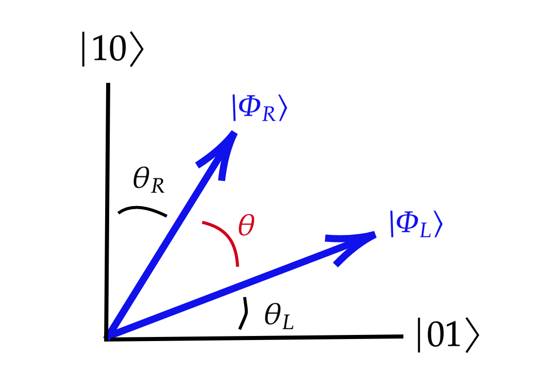
Figure 5: Schematic representation of the new unconstrained search approach introduced in this work. Here we represent the two vectors needed to find the universal functional of the Bose-Hubbard dimer with 2 bosons (see Eq. (38)). The vectors $|\Phi_{L}\rangle$ and $|\Phi_{R}\rangle$ live in $\mathcal{H}_{1}$, the Hilbert space of 1 particle. The basis of the space is $\{\mbox{$|01\rangle$},\mbox{$|10\rangle$}\}$. The minimum of the functional (39) is attained when $\theta_{L}=\theta_{R}=(\pi/2-\theta)/2$, and the value of the functional is found to be $\mathcal{F}(\theta)=2\sin^{2}(\pi/4-\theta/2)=1-\sin(\theta)$.

B.3 The unconstrained search approach for the Bose-Hubbard dimer

In this section we focus on the case $N=2$ for the Boson-Hubbard dimer, whose Hamiltonian reads ($U>0$)

$$H=-t(b_{L}^{\dagger}b_{R}+b_{R}^{\dagger}b_{L})+\frac{U}{2}\!\sum_{j=L/R}\!\hat{n}_{j}(\hat{n}_{j}-1),$$ (35)

where the operators $b^{\dagger}_{j}$ and $b_{j}$ create and annihilate a boson on the sites $j=L/R$, and $\hat{n}_{j}$ is the corresponding particle-number operator. The dimension of the Hilbert space is 3 with basis set $\{\mbox{$|2,0\rangle$},\mbox{$|1,1\rangle$},\mbox{$|0,2\rangle$}\}$, with the configuration states defined by:

$$\mbox{$|n,N-n\rangle$}=\frac{1}{\sqrt{n!(N-n)!}}(b^{\dagger}_{L})^{n}(b^{\dagger}_{R})^{N-n}\mbox{$|0\rangle$}.$$ (36)

The ground state belonging to such a space reads: $\mbox{$|\Psi\rangle$}=\alpha_{0}\mbox{$|2,0\rangle$}+\alpha_{1}\mbox{$|1,1\rangle$}+\alpha_{0}\mbox{$|0,2\rangle$}$. The functional to be optimized is:

$$\mathcal{J}[\Phi_{L},\Phi_{R}]=\mbox{$\langle\Phi_{L}|$}\hat{n}_{L}\mbox{$|\Phi_{L}\rangle$}+\mbox{$\langle\Phi_{R}|$}\hat{n}_{R}\mbox{$|\Phi_{R}\rangle$}\,,$$ (37)

such that $\mbox{$|\Phi_{i}\rangle$}\in\mathcal{H}_{1}$, $\mbox{$\langle\Phi_{L}|$}\Phi_{R}\rangle=\gamma_{LR}$ and $\mbox{$\langle\Phi_{i}|$}\Phi_{i}\rangle=1$. We can write (see Fig. 5):

$$\mbox{$|\Phi_{L}\rangle$}=\cos(\theta_{L})\mbox{$|0,1\rangle$}+\sin(\theta_{L})\mbox{$|1,0\rangle$}\qquad{\rm and}\qquad\mbox{$|\Phi_{R}\rangle$}=\cos(\theta_{R})\mbox{$|1,0\rangle$}+\sin(\theta_{R})\mbox{$|0,1\rangle$}.$$ (38)

Therefore $\mbox{$\langle\Phi_{L}|$}\Phi_{R}\rangle=\cos(\theta_{L})\sin(\theta_{R})+\sin(\theta_{L})\cos(\theta_{R})$. By defining $\gamma_{LR}=\cos(\theta)$, we have $\sin(\theta_{L}+\theta_{R})=\cos(\theta)$. As a result, $\theta_{L}+\theta_{R}+\theta=\pi/2$, and $\sin(\theta_{R})=\cos(\theta_{L}+\theta)$. Our functional (37) then reads:

$$\mathcal{J}(\theta,\theta_{L})=\sin^{2}(\theta_{L})+\cos^{2}(\theta+\theta_{L}).$$ (39)

The minimum is attached when $d\mathcal{J}(\theta,\theta_{L})/d\theta_{L}=0$. An elementary calculation gives as a solution $\sin^{2}(2\theta_{L}^{*})=\cos^{2}(\theta)$ for the minimizer $\theta_{L}^{*}$, which results in

$$\mathcal{F}(\theta)=\mathcal{J}(\theta,\theta_{L}^{*}) =\sin^{2}(\theta^{*}_{L})+\cos^{2}(\theta)\cos^{2}(\theta^{*}_{L})+\sin^{2}(\theta^{*}_{L})\sin^{2}(\theta)-\cos^{3}(\theta)\sin(\theta)$$

$$=1-\sin(\theta)=1-\sqrt{1-\cos^{2}(\theta)}=1-\sqrt{1-\gamma_{LR}^{2}}\,,$$ (40)

which is the result found several times in the literature for bosons and fermions Cohen and Mori-Sánchez (2016); Töws and Pastor (2011); Carrascal et al. (2015); Benavides-Riveros et al. (2020). We compare the function in Eq. (39) w.r.t. the solution of Eq. (40) in Fig. 6 for $\theta=2\pi/7$.

There is still a quicker way of computing the same result. In $\mathcal{H}_{1}$ the number operators can be written as $\hat{n}_{L}=\mbox{$|10\rangle$}\mbox{$\langle 10|$}$ and $\hat{n}_{R}=\mbox{$|01\rangle$}\mbox{$\langle 01|$}$. Hence, it is obvious that the minimum of (39) is reached when $\theta_{L}=\theta_{R}=(\pi/2-\theta)/2$ and the value of the functional is just $2\sin^{2}[(\pi/2-\theta)/2]=1-\sin(\theta)$.

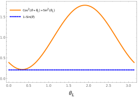
Figure 6: Plot of the unconstrained search for $\gamma_{LR}=\cos(\theta)$ with $\theta=2\pi/7$. The minimum of the functional (39) is reached at $\theta_{L}^{*}=3\pi/28$ and the value of the functional is $0.21$.

B.4 The unconstrained search approach for large number of modes

Expanded in a basis for $\mathcal{G}_{\gamma}$ the kets in Eq. (25) can be written as

$$\mbox{$|\Phi^{\prime}_{\gamma,i}\rangle$}=\sum_{\mathbf{m}}d_{i,\mathbf{m}}\mbox{$|\mathbf{m}\rangle$}\,.$$ (41)

Then, for each $\gamma$ there is a square matrix $\mathbf{d}_{i,\mathbf{m}}$ that can be singular-value decomposed as $\mathbf{d}=\mathbf{U}\mathbf{D}\mathbf{V}^{\dagger}$, where $\mathbf{U}$ is an $M\times M$ complex unitary matrix, $\mathbf{D}$ is an $M\times M$ diagonal matrix with non-negative real numbers on the diagonal, and $\mathbf{V}$ is a $M\times M$ complex unitary matrix. The non-diagonal entries of the corresponding 1RDM $\gamma$ can be computed as:

$$\gamma_{ij}=\mbox{$\langle\Psi|$}b^{\dagger}_{i}b_{j}\mbox{$|\Psi\rangle$}=\langle\Phi_{\gamma,i}\mbox{$|\Phi_{\gamma,j}\rangle$}\,.$$ (42)

Hence,

$$\gamma=\mathbf{d}\mathbf{d}^{\dagger}=\mathbf{U}\mathbf{D}\mathbf{V}^{\dagger}\mathbf{V}\mathbf{D}^{T}\mathbf{U}^{\dagger}=\mathbf{U}\mathbf{D}\mathbf{D}^{T}\mathbf{U}^{\dagger}.$$ (43)

Therefore $\mathbf{D}\mathbf{D}^{\dagger}=\mathbf{U}^{\dagger}\gamma\mathbf{U}$. As a consequence, $\mathbf{U}$ diagonalizes the matrix $\gamma$, and $\mathbf{D}\mathbf{D}^{T}$ is a diagonal matrix with the eigenvalues of $\gamma$ in the entries. Therefore the diagonal entries of $\mathbf{D}$ are $\sqrt{n_{1}},\sqrt{n_{2}},...,\sqrt{n_{M}}$, the square root of the eigenvalues of $\gamma$. The kets in Eq. (41) can then be explicitly written as functions of $\gamma$:

$$\mbox{$|\Phi_{\gamma,i}\rangle$}=\sum_{\alpha,\mathbf{m}}u_{i\alpha}\sqrt{n_{\alpha}}v_{\mathbf{m},\alpha}^{*}\mbox{$|\mathbf{m}\rangle$}\,.$$ (44)

The connection with the original wave function is striking:

$$\mbox{$|\Psi_{\gamma}\rangle$}=\frac{1}{N}\sum_{i}b^{\dagger}_{i}\mbox{$|\Phi_{\gamma,i}\rangle$}=\frac{1}{N}\sum_{i}b^{\dagger}_{i}\sum_{\alpha,\mathbf{m}}u_{i\alpha}\sqrt{n_{\alpha}}v_{\mathbf{m},\alpha}^{*}\mbox{$|\mathbf{m}\rangle$}=\frac{1}{N}\sum_{\alpha}\sqrt{n_{\alpha}}\,\tilde{b}^{\dagger}_{\alpha}\mbox{$|v_{\alpha}\rangle$}\,,$$ (45)

where $\tilde{b}^{\dagger}_{\alpha}=\sum_{i}b^{\dagger}_{i}u_{i\alpha}$ and $\mbox{$|v_{\alpha}\rangle$}=\sum_{\mathbf{m}}v_{\mathbf{m},\alpha}^{*}\mbox{$|\mathbf{m}\rangle$}$. Notice that the 1RDM $\gamma$ fixes $\tilde{b}^{\dagger}_{\alpha}$ and $\sqrt{n_{\alpha}}$, but not $|v_{\alpha}\rangle$. Quite remarkable, we can recognize in the expression (45) the well-known Schmidt decomposition of a bipartite system: in this case the system of 1 and $(N-1)$ indistinguishable particles. Such a decomposition can be used to study fermionic entanglement as quantum resource Gigena et al. (2020); Lo Franco and Compagno (2018) or to describe the correlated electron dynamics in strong laser fields within exact factorization of the wave function Schild and Gross (2017). As its is discussed in Section C, the matrix $\mathbf{V}$ is used to engineer the bosonic functionals by training a neural network to produce $\mathbf{V}$ as a function of $\gamma$.

Appendix C Neural Networks

The hyperparameters used in our neural networks are the following:

Hyperparameters:	N=2,M=2	N=4, M=4
optimizer	AdamW	AdamW
momentum	0.9	0.9
weight-decay	1e-06	1e-06
learningrate	0.00003	0.00001
epochs	10000	20000
hidden layer size	20, 20	400, 400

References

- Hohenberg and Kohn (1964) P. Hohenberg and W. Kohn, “Inhomogeneous electron gas,” Phys. Rev. 136, B864 (1964).
- Jones (2015) R. O. Jones, “Density functional theory: Its origins, rise to prominence, and future,” Rev. Mod. Phys. 87, 897 (2015).
- Cazalilla et al. (2011) M. A. Cazalilla, R. Citro, T. Giamarchi, E. Orignac, and M. Rigol, “One dimensional bosons: From condensed matter systems to ultracold gases,” Rev. Mod. Phys. 83, 1405 (2011).
- Chatterjee et al. (2020) B. Chatterjee, C. Lévêque, J. Schmiedmayer, and A. U.J. Lode, “Detecting One-Dimensional Dipolar Bosonic Crystal Orders via Full Distribution Functions,” Phys. Rev. Lett. 125, 093602 (2020).
- González-Cuadra et al. (2018) D. González-Cuadra, P. R. Grzybowski, A. Dauphin, and M. Lewenstein, “Strongly Correlated Bosons on a Dynamical Lattice,” Phys. Rev. Lett. 121, 090402 (2018).
- Fisher et al. (1989) M. P. A. Fisher, P. B. Weichman, G. Grinstein, and D. S. Fisher, “Boson localization and the superfluid-insulator transition,” Phys. Rev. B 40, 546 (1989).
- Pitaevskii and Stringari (2003) L. P. Pitaevskii and S. Stringari, Bose-Einstein Condensation (Clarendon Press, 2003).
- Dalfovo et al. (1999) F. Dalfovo, S. Giorgini, L. Pitaevskii, and S. Stringari, “Theory of Bose-Einstein condensation in trapped gases,” Rev. Mod. Phys. 71, 463 (1999).
- Gubernatis et al. (2016) J. Gubernatis, N. Kawashima, and P. Werner, Quantum Monte Carlo Methods: Algorithms for Lattice Models (Cambridge University Press, 2016).
- Saito (2017) H. Saito, “Solving the Bose-Hubbard Model with Machine Learning,” J. Phys. Soc. Jpn. 86, 093001 (2017).
- Choo et al. (2018) K. Choo, G. Carleo, N. Regnault, and T. Neupert, “Symmetries and Many-Body Excitations with Neural-Network Quantum States,” Phys. Rev. Lett. 121, 167204 (2018).
- Bloch et al. (2008) I. Bloch, J. Dalibard, and W. Zwerger, “Many-body physics with ultracold gases,” Rev. Mod. Phys. 80, 885 (2008).
- Chin et al. (2010) C. Chin, R. Grimm, P. Julienne, and E. Tiesinga, “Feshbach resonances in ultracold gases,” Rev. Mod. Phys. 82, 1225 (2010).
- Bloch (2005) I. Bloch, “Ultracold quantum gases in optical lattices,” Nature Phys. 1, 23–30 (2005).
- Gross and Bloch (2017) C. Gross and I. Bloch, “Quantum simulations with ultracold atoms in optical lattices,” Science 357, 995 (2017).
- Schäfer et al. (2020) F. Schäfer et al., “Tools for quantum simulation with ultracold atoms in optical lattices,” Nature Rev. Phys. 2, 411 (2020).
- Schmied et al. (2016) R. Schmied et al., “Bell correlations in a Bose-Einstein condensate,” Science 352, 441 (2016).
- Fadel et al. (2018) M. Fadel et al., “Spatial entanglement patterns and Einstein-Podolsky-Rosen steering in Bose-Einstein condensates,” Science 360, 409 (2018).
- Kunkel et al. (2018) P. Kunkel et al., “Spatially distributed multipartite entanglement enables EPR steering of atomic clouds,” Science 360, 413 (2018).
- Lange et al. (2018) K. Lange et al., “Entanglement between two spatially separated atomic modes,” Science 360, 416 (2018).
- Benavides-Riveros et al. (2020) C. L. Benavides-Riveros, J. Wolff, M. A. L. Marques, and C. Schilling, “Reduced Density Matrix Functional Theory for Bosons,” Phys. Rev. Lett. 124, 180603 (2020).
- Liebert and Schilling (2021) J. Liebert and C. Schilling, “Functional Theory for Bose-Einstein Condensates,” Phys. Rev. Research 3, 013282 (2021).
- Gilbert (1975) T. Gilbert, “Hohenberg-Kohn theorem for nonlocal external potentials,” Phys. Rev. B 12, 2111 (1975).
- Pernal and Giesbertz (2016) K. Pernal and K. J. H. Giesbertz, “Reduced density matrix functional theory (RDMFT) and linear response time-dependent RDMFT,” Top. Curr. Chem. 368, 125 (2016).
- Sakmann et al. (2008) K. Sakmann, A. I. Streltsov, O. E. Alon, and L. S. Cederbaum, “Reduced density matrices and coherence of trapped interacting bosons,” Phys. Rev. A 78, 023615 (2008).
- Bulgac and Jin (2017) A. Bulgac and S. Jin, “Dynamics of Fragmented Condensates and Macroscopic Entanglement,” Phys. Rev. Lett. 119, 052501 (2017).
- Aloy et al. (2021) A. Aloy, M. Fadel, and J. Tura, “The quantum marginal problem for symmetric states: applications to variational optimization, nonlocality and self-testing,” New J. Phys. 23, 033026 (2021).
- Walter et al. (2013) M. Walter et al., “Entanglement polytopes: Multiparticle entanglement from single-particle information,” Science 340, 1205 (2013).
- Sawicki et al. (2014) A. Sawicki, M. Oszmaniec, and M. Kuś, “Convexity of momentum map, Morse index, and quantum entanglement,” Rev. Math. Phys. 26, 1450004 (2014).
- Sawicki et al. (2012) A. Sawicki, M. Oszmaniec, and M. Kuś, “Critical sets of the total variance can detect all stochastic local operations and classical communication classes of multiparticle entanglement,” Phys. Rev. A 86, 040304(R) (2012).
- Yu et al. (2021) X. Yu et al., “A complete hierarchy for the pure state marginal problem in quantum mechanics,” Nature Comm. 12, 1012 (2021).
- Kalita et al. (2021) B. Kalita, L. Li, R. J. McCarty, and K. Burke, “Learning to approximate density functionals,” Acc. Chem. Res. 54, 818 (2021).
- Brockherde et al. (2017) F. Brockherde, L. Vogt, L. Li, M. Tuckerman, K. Burke, and K.-R. Müller, “Bypassing the Kohn-Sham equations with machine learning,” Nat. Comm. 8, 872 (2017).
- Schmidt et al. (2019a) J. Schmidt, C. L. Benavides-Riveros, and M. A. L. Marques, “Machine Learning the Physical Nonlocal Exchange-Correlation Functional of Density-Functional Theory,” J. Phys. Chem. Lett. 10, 6425 (2019a).
- Li et al. (2021) L. Li, S. Hoyer, R. Pederson, R. Sun, E.D. Cubuk, Riley P., and K. Burke, “Kohn-Sham Equations as Regularizer: Building Prior Knowledge into Machine-Learned Physics,” Phys. Rev. Lett. 126, 036401 (2021).
- Margraf and Reuter (2021) J. Margraf and K. Reuter, “Pure non-local machine-learned density functional theory for electron correlation,” Nature Comm. 12, 344 (2021).
- Moreno et al. (2020) J. R. Moreno, G. Carleo, and A. Georges, “Deep Learning the Hohenberg-Kohn Maps of Density Functional Theory,” Phys. Rev. Lett. 125, 076402 (2020).
- Gibney et al. (2021) D. Gibney, J.-N. Boyn, and D. Mazziotti, “Toward a Resolution of the Static Correlation Problem in Density Functional Theory from Semidefinite Programming,” J. Phys. Chem. Lett. 12, 385 (2021).
- Levy (1979) M. Levy, “Universal variational functionals of electron densities, first-order density matrices, and natural spin-orbitals and solution of the v-representability problem,” Proc. Natl. Acad. Sci. U.S.A 76, 6062 (1979).
- Schilling et al. (2020) C. Schilling, C. L. Benavides-Riveros, A. Lopes, T. Maciażek, and A. Sawicki, “Implications of pinned occupation numbers for natural orbital expansions: I. Generalizing the concept of active spaces,” New J. Phys. 22, 023001 (2020).
- Löwdin and Shull (1956) P.-O. Löwdin and H. Shull, “Natural orbitals in the quantum theory of two-electron systems,” Phys. Rev. 101, 1730 (1956).
- Schilling and Schilling (2019) C. Schilling and R. Schilling, “Diverging Exchange Force and Form of the Exact Density Matrix Functional,” Phys. Rev. Lett. 122, 013001 (2019).
- Giesbertz (2020) K. J. H. Giesbertz, “Implications of the unitary invariance and symmetry restrictions on the development of proper approximate one-body reduced-density-matrix functionals,” Phys. Rev. A 102, 052814 (2020).
- Fadel et al. (2020) M. Fadel, A. Aloy, and J. Tura, “Bounding the fidelity of quantum many-body states from partial information,” Phys. Rev. A 102, 020401(R) (2020).
- Mori-Sánchez and Cohen (2018) P. Mori-Sánchez and A. J. Cohen, “Exact Density Functional Obtained via the Levy Constrained Search,” J. Phys. Chem. Lett. 9, 4910 (2018).
- Giesbertz and Ruggenthaler (2019) K. J. H. Giesbertz and M. Ruggenthaler, “One-body reduced density-matrix functional theory in finite basis sets at elevated temperatures,” Phys. Rep. 806, 1 (2019).
- Jaksch et al. (1998) D. Jaksch, C. Bruder, J. I. Cirac, C. W. Gardiner, and P. Zoller, “Cold Bosonic Atoms in Optical Lattices,” Phys. Rev. Lett. 81, 3108 (1998).
- Cohen and Mori-Sánchez (2016) A. J. Cohen and P. Mori-Sánchez, “Landscape of an exact energy functional,” Phys. Rev. A 93, 042511 (2016).
- Töws and Pastor (2011) W. Töws and G. M. Pastor, “Lattice density functional theory of the single-impurity Anderson model: Development and applications,” Phys. Rev. B 83, 235101 (2011).
- Carleo et al. (2019) G. Carleo, I. Cirac, K. Cranmer, L. Daudet, M. Schuld, N. Tishby, L. Vogt-Maranto, and L. Zdeborová, “Machine learning and the physical sciences,” Rev. Mod. Phys. 91, 045002 (2019).
- Carrasquilla (2020) J. Carrasquilla, “Machine learning for quantum matter,” Adv. Phys. X 5, 1797528 (2020).
- Müller (1984) A. M. K. Müller, “Explicit approximate relation between reduced two- and one-particle density matrices,” Phys. Lett. A 105, 446 (1984).
- Buijse and Baerends (2002) M. Buijse and E. Baerends, “An approximate exchange-correlation hole density as a functional of the natural orbitals,” Mol. Phys. 100, 401 (2002).
- Frank et al. (2007) R. L. Frank, E. H. Lieb, R. Seiringer, and H. Siedentop, “Müller’s exchange-correlation energy in density-matrix-functional theory,” Phys. Rev. A 76, 052517 (2007).
- Benavides-Riveros and Marques (2018) C. L. Benavides-Riveros and M. A. L. Marques, “Static correlated functionals for reduced density matrix functional theory,” Eur. Phys. J. B 91, 133 (2018).
- Benavides-Riveros and Marques (2019) C. L. Benavides-Riveros and M. A. L. Marques, “On the time evolution of fermionic occupation numbers,” J. Chem. Phys. 151, 044112 (2019).
- Lezcano-Casado (2019) M. Lezcano-Casado, “Trivializations for gradient-based optimization on manifolds,” in Advances in Neural Information Processing Systems, NeurIPS (2019) pp. 9154–9164.
- Siegel (2020) J. Siegel, “Accelerated Optimization with Orthogonality Constraints,” J. Comput. Math. 39, 207 (2020).
- Paszke et al. (2017) A. Paszke et al., “Automatic differentiation in pytorch,” in NIPS 2017 Autodiff Workshop: The Future of Gradient-based Machine Learning Software and Techniques (2017).
- (60) “Geotorch,” https://github.com/Lezcano/geotorch.
- Maciażek (2021) T. Maciażek, “Universality of the Bose-Einstein condensation force in the Reduced Density Matrix Functional Theory,” (2021), arXiv:2103.17069 .
- Clevert et al. (2015) D.-A. Clevert, T. Unterthiner, and S. Hochreiter, “Fast and Accurate Deep Network Learning by Exponential Linear Units (ELUs),” arXiv:1511.07289 (2015).
- Wang et al. (2009) F. Wang, F. Pollmann, and A. Vishwanath, “Extended Supersolid Phase of Frustrated Hard-Core Bosons on a Triangular Lattice,” Phys. Rev. Lett. 102, 017203 (2009).
- Hunter et al. (2020) A. L. Hunter, M. T. Eiles, A. Eisfeld, and J. M. Rost, “Rydberg Composites,” Phys. Rev. X 10, 031046 (2020).
- Schmidt et al. (2019b) J. Schmidt, C. L. Benavides-Riveros, and M. A. L. Marques, “Representability problem of density functional theory for superconductors,” Phys. Rev. B 99, 024502 (2019b).
- Schmidt et al. (2019c) J. Schmidt, C. L. Benavides-Riveros, and M. A. L. Marques, “Reduced density matrix functional theory for superconductors,” Phys. Rev. B 99, 224502 (2019c).
- Alon et al. (2005) O. E. Alon, A. I. Streltsov, and L. S. Cederbaum, “Zoo of Quantum Phases and Excitations of Cold Bosonic Atoms in Optical Lattices,” Phys. Rev. Lett. 95, 030405 (2005).
- Mazziotti and Herschbach (1999) D. A. Mazziotti and D. R. Herschbach, “Boson correlation energies from reduced hamiltonian interpolation,” Phys. Rev. Lett. 83, 5185 (1999).
- Gidofalvi and Mazziotti (2004) G. Gidofalvi and D. A. Mazziotti, “Boson correlation energies via variational minimization with the two-particle reduced density matrix: Exact -representability conditions for harmonic interactions,” Phys. Rev. A 69, 042511 (2004).
- Lieb and Seiringer (2009) E. H. Lieb and R. Seiringer, The Stability of Matter in Quantum Mechanics (Cambridge University Press, 2009).
- Klyachko (2006) A. Klyachko, “Quantum marginal problem and N-representability,” J. Phys. Conf. Ser. 36, 72 (2006).
- Reuvers (2021) R. Reuvers, “Generalized Pauli constraints in large systems: The Pauli principle dominates,” J. Math. Phys. 62, 032204 (2021).
- Carrascal et al. (2015) D. Carrascal, J. Ferrer, J. Smith, and K. Burke, “The Hubbard dimer: a density functional case study of a many-body problem,” J. Phys. Condens. Matter 27, 393001 (2015).
- Gigena et al. (2020) N. Gigena, M. Di Tullio, and R. Rossignoli, “One-body entanglement as a quantum resource in fermionic systems,” Phys. Rev. A 102, 042410 (2020).
- Lo Franco and Compagno (2018) R. Lo Franco and G. Compagno, “Indistinguishability of Elementary Systems as a Resource for Quantum Information Processing,” Phys. Rev. Lett. 120, 240403 (2018).
- Schild and Gross (2017) A. Schild and E. K. U. Gross, “Exact Single-Electron Approach to the Dynamics of Molecules in Strong Laser Fields,” Phys. Rev. Lett. 118, 163202 (2017).