remarkRemark \newsiamremarkhypothesisHypothesis \newsiamthmclaimClaim \headersUpscaling errors for the Landau-Lifshitz equationL. Leitenmaier and O. Runborg
Upscaling errors in Heterogeneous Multiscale Methods for the Landau-Lifshitz equation
Abstract
In this paper, we consider several possible ways to set up Heterogeneous Multiscale Methods for the Landau-Lifshitz equation with a highly oscillatory diffusion coefficient, which can be seen as a means to modeling rapidly varying ferromagnetic materials. We then prove estimates for the errors introduced when approximating the relevant quantity in each of the models given a periodic problem, using averaging in time and space of the solution to a corresponding micro problem. In our setup, the Landau-Lifshitz equation with highly oscillatory coefficient is chosen as the micro problem for all models. We then show that the averaging errors only depend on , the size of the microscopic oscillations, as well as the size of the averaging domain in time and space and the choice of averaging kernels.
keywords:
Heterogeneous Multiscale Methods; Micromagnetics; Magnetization Dynamics;65M15; 35B27; 78M40
1 Introduction
In micromagnetics, the evolution of the magnetization within a ferromagnet is described by the Landau-Lifshitz (LL) equation [16]. In this paper, we consider a simplification of the deterministic version of this equation, where we only take into account the exchange interaction between magnetic moments and neglect other contributions influencing the magnetization, such as anisotropy, temperature and external field. We consider a ferromagnet with a rapidly varying material, which we model by introducing a material coefficient , where represents the spatial scale of the finest variations.. One example could be a composite, consisting of two different materials with different interaction behavior and layers of thickness . According to this simplified model, the partial differential equation determining the evolution of the magnetization then is
| (1) |
where is a smooth function with values in such that , and a damping coefficient. In this model, the effective field is given by
| (2) |
Here the coefficient influences the overall behavior of the magnetization significantly. A very similar model was first introduced in [13] and used recently in [2]. Also in for example [19] and [8], related approaches are applied.
When solving 1 numerically, one would have to resolve the -scale in order to get a correct result. However, the resulting amount of computational work is infeasible for small . Instead of solving 1, one therefore in many cases considers solutions to a corresponding effective equation instead, which capture the correct magnetization behavior on a coarse scale but do not resolve the -scale. For periodic problems, one can apply techniques from classic homogenization theory, [9], [7], to obtain such a homogenized solution as well as correction terms as shown in [17]. When aiming to deal with somewhat more general coefficients, though, it can be advantageous to instead use numerical methods to approximate the homogenized solution. This can be done using multiscale methods like equation free methods [14] or heterogeneous multiscale methods (HMM) [20], [21], [1]. The basic idea of HMM is to combine a coarse scale macro model, that involves some unknown quantity, with micro problems that are solved on a short time interval and small domain only. In the so-called upscaling process, the solution from the micro problem is then averaged to obtain the quantity that is needed to complete the macro model. This is the approach that we consider in this paper. In particular, we choose three different HMM macro models for 1. For the case of a periodic material coefficient, we then investigate the upscaling error for each of the models, in order to get an understanding of what are good ways to set up HMM for this problem. We come to the conclusion that all three models give very similar results and can thus be valid choices for HMM setups. Which model to choose can thus mostly be based on advantages related to the numerical implementation.
HMM has previously been applied to a Landau-Lifshitz problem in [3], [4]. However, in these articles, the authors do not consider the case with a material coefficient that is highly oscillatory in space, 1, but instead a highly oscillatory external field with temporal oscillations.
In the remainder of this section, we shortly introduce some of the notation that is used in the following. We furthermore describe the homogenized solution for 1 with a periodic material coefficient as derived in [17], which will subsequently act as a reference. We continue in Section 2 by describing the concept of heterogeneous multiscale methods as well as the models considered. In Section 3, estimates for the homogenized solution and the corresponding correctors to the HMM micro problem are stated to provide the basis that is required for the subsequent derivations. We moreover add an explicit description of a particular correction term. In Section 4, we derive several lemmas regarding the averaging required for numerical homogenization. These lay the ground for the error estimates for the different upscaling-models, which are given in Section 5 and constitute the main result of this paper. Finally, in Section 6 we present several numerical examples in one and two space dimensions which show the validity of the theoretical estimates.
1.1 Preliminaries
We consider -periodic solutions to 1 in the -dimensional hypercube and time interval , for some . We use to denote the -dimensional unit cell and let for a parameter .
We denote by the standard periodic Sobolev spaces on and by periodic Bochner-Sobolev spaces on . The corresponding norms are and . Furthermore, and denote standard Sobolev spaces, being the Sobolev supremum norm on : given for a multi-index with , it holds that
Furthermore, we make frequent use of the Sobolev inequality stating that given for dimension , it holds that
| (3) |
In general, we use capital letters to refer to solutions on the whole domain and for time , . When instead considering a micro problem set on , we use lower case letters to denote the solution. By we denote the Jacobian matrix of the vector-valued function . We assume in general that scalar and cross product between a vector-valued and a matrix-valued function are done column-wise, while the divergence operator is applied row-wise.
The differential operator is defined such that for ,
| (4) |
where is a highly oscillatory, smooth, scalar coefficient function. Moreover, we denote by the corresponding operator acting on vector-valued functions in ,
where is the -th component of .
1.2 Homogenized equation for the periodic problem
The homogenization of 1 with a periodic material coefficient was studied in [17]. Using the setup considered there makes it possible to obtain bounds for the errors introduced when using HMM. It therefore is the scenario that we focus on in the subsequent proofs. Specifically, we assume that satisfies 1 with on a domain , where or 3 and , and for . Then it is shown in [17] that the corresponding homogenized equation is
| (5a) | ||||
| (5b) | ||||
for and . The constant homogenized coefficient matrix is as in elliptic homogenization theory given by
| (6) |
where is the solution to the elliptic cell problem
| (7) |
Note that 7 determines only up to a constant. Throughout this article, we assume that this constant is chosen such that has zero average.
For the difference between and , the following result was proved in [17].
Theorem 1.1.
Assume that is a classical solution to 1 with a periodic material coefficient where and that for some constants . Assume that there is a constant independent of such that for . Moreover, suppose that is a classical solution to 5. We then have
| (8) |
where the constant is independent of and but depends on and .
2 Heterogeneous multiscale methods
The concept of heterogeneous multiscale methods was first introduced by E and Engquist in [20]. It provides a general approach to treat multiscale problems with scale separation, where a description of the microscopic problem is available but would be too computationally expensive to use throughout the whole domain. The idea is therefore to use numerical homogenization with the goal to get a good approximation to the effective solution of the original problem. In general, HMM models involve three parts:
-
1.
Macro model: an incomplete model for the whole computational domain, discretized with a coarse grid, that is set up in such a way that some data is missing.
-
2.
Micro model: an exact model discretized with a grid resolving the fine -scale, which is however only solved on a small domain, where it is feasible to use the expensive description.
-
3.
Upscaling: an averaging procedure that uses the data obtained when solving the micro problem to generate the quantity needed to complete the macro model.
It is important to make sure that micro and macro model are consistent, which is typically achieved by choosing the initial data for the micro problem as a restriction of the current macro solution.
The HMM framework has been successfully applied to a wide range of applications; see for instance the surveys in [21, 1]. In this paper, we aim to find a good way to set up HMM for the Landau Lifshitz equation 1.
In general, the error in the HMM solution consists of two major components apart from discretization errors: an error term related to the fact that the solution to the effective equation is approximated instead of the original one and the so-called HMM error. The HMM error in turn depends on the upscaling error, the error introduced in the data estimation process [1]. In case of the Landau-Lifshitz equation with a periodic material coefficient, an estimate for the first error term is given by Theorem 1.1. The -homogenization error is . In this paper, we focus on estimates for the upscaling error and investigate how it is influenced by different choices of HMM-models.
We consider three different setups. All three are based on the same micro model, the full Landau-Lifshitz equation,
| (9a) | ||||
| (9b) | ||||
with periodic boundary conditions. The initial data is assumed to be a restriction of the macro data such that the micro and macro model are consistent and . One possible choice to obtain such initial data is by using a normalized interpolation polynomial based on the macro data. In this paper, we assume a solution to the micro problem in the whole domain with periodic boundary conditions. In practice, one would solve the micro problem only on a small domain , where . However, this requires a choice of boundary conditions which introduce some additional error. To simplify the following analysis, we avoid dealing with this issue here and assume a solution in the whole domain. For the averaging we then consider only the solution in a box in space and an interval in time, where and . This matches the scales of the fast variations in the problem as explained in [17].
The other two HMM components, macro model and upscaling, differ between the models. We suppose that the macro models should have the general form of the effective equation 5 and consider three different choices of missing data in the model as described in the following.
-
(M1)
Flux model. We choose the macro model
(10a) (10b) where the missing information to complete the model is the flux . In case of a periodic material coefficient, would ideally be . Then 10 coincides with 5. To obtain , we average the product of the material coefficient and gradient of the solution to the micro problem in space and time using averaging kernels as explained in more detail in Section 4,
-
(M2)
Field model. Here the macro model is given by
where takes the role of the effective field. In the periodic case, should hence approximate . In general, is defined as the average of the operator applied to the solution to the micro problem,
-
(M3)
Torque model. The third macro model we consider is
which means that for a periodic material coefficient, should approximate the torque . Here is given by
In the following, we prove estimates for the upscaling error in each of the three models, (M1) - (M3), when is periodic,
under the assumption that for multi-indices with , where is the macro point we average around.
3 Homogenized solution and correctors for a periodic micro problem
To be able to prove estimates for the upscaling errors - given a periodic material coefficient, we make use of the estimates for the error between the actual and the homogenized solution to 9 as well as the corresponding corrected approximations that were derived in [17].
Let be the solution to 9 given . Then, according to [17], the corresponding homogenized solution is , which for satisfies
| (11a) | ||||
| (11b) | ||||
with periodic boundary conditions and where is chosen as in 9.
We consider a short time interval , with an -dependent final time
| (12) |
This is still sufficiently long time for the HMM micro problems with final time . In [17], it is shown that for such a time interval, one obtains improved approximations to the solution to 9, , when not only considering but a truncated asymptotic expansion
| (13) |
where the correctors , satisfy linear differential equations in the fast variables and ,
Here the forcing depends only on the lower order terms , . The operator is the vector-equivalent to , which is defined such that for ,
| (15) |
As explained in [17], the form of the first corrector is
| (16) |
where is the solution to 7 and is an oscillatory, decaying term that is discussed in Section 3.2.
3.1 Energy and error estimates
For convenience of the reader, we here give a summary of the estimates from [17] that are most crucial for the derivations in this paper. In contrast to [17], we here require higher regularity of for reasons of simplicity. Otherwise we use the same assumptions. In particular, we assume that
-
(A1)
the material coefficient is a periodic function such that there are positive constants satisfying .
-
(A2)
the initial data function is normalized, , which implies that for any . From this property it follows that given a multi-index with ,
and thus and are orthogonal.
-
(A3)
the damping coefficient is positive and it holds that . Moreover, for some , which implies .
-
(A4)
with is a classical solution to 9 and there is a constant independent of such that
-
(A5)
is a classical solution to 11.
As shown in [17], it then holds for any that the -norms of the first two correctors, and , are bounded uniformly in the fast time variable , while the norms of higher order correctors grow algebraically with . Specifically, it holds for all and that
| (17) |
where the constant depends on but is independent of . For the approximating in 13, it holds for that
| (18) |
Moreover, consider the error introduced when approximating by . Under the given assumptions, it holds for and that
| (19) |
where the constant is independent of but depends on in (A4) and . This estimate shows that the approximations improve with increasing on the considered time interval.
3.2 The correction term
In [17], it was shown that both and the correction term , which is part of as given in 16, are orthogonal to ,
| (20) |
Moreover, it was proved that given (A1)-(A5), there are constants and independent of such that
| (21) |
For the analysis in this paper, an explicit formulation for is required. To obtain such a description, we use the linear equation that was derived in [17],
| (22a) | ||||
| (22b) | ||||
We now introduce a lemma that shows a connection between differential equations of the same type as 22 to a system of parabolic equations that become Schrödinger equations as . Then we go on and use that result to derive an explicit solution to 22 in terms of the eigenfunctions of the operator .
Lemma 3.1.
Suppose and is a given constant vector with . Then the solution to
| (23) |
with periodic boundary conditions is given by
| (24) |
where solves
| (25) |
with periodic boundary conditions.
Proof 3.2.
As is real, it follows immediately that given by 24 satisfies the initial condition in 23. Moreover, since is constant,
where we used the vector triple product identity for the last step. It then follows that
It thus holds that
Using 25 and exploiting the facts that is constant and is independent of time, we obtain
In the following, let be the eigenfunctions and eigenvalues of the operator , where is given by 15, on with periodic boundary conditions,
As is a periodic elliptic operator it holds according to standard theory that its eigenvalues are strictly positive and bounded away from zero except for the first eigenvalue, , which is zero [15],
Moreover, the eigenfunctions form an orthonormal basis for . In particular, the first eigenfunction, corresponding to , is the constant function . The eigenfunctions can be chosen to be real, which they are assumed to be in the following. We then obtain the following expression for the correction term .
Lemma 3.3.
Let and
| (26) |
where and , , are the eigenfunctions and eigenvalues of and are expansion coefficients such that . Then
solves 22 .
Proof 3.4.
Since satisfies a linear differential equation in the fast variables, we write and suppress the dependence on the slow variables, and , in the notation throughout this proof. Note also that with respect to the fast variables only, and are constant.
By Lemma 3.1 and using the fact that by (A2), and are orthogonal to each other, we find that the solution to 22 is
| (27) |
where is the solution to
| (28) |
As 28 is a system of three decoupled equations, we can consider each equation separately and solve it in terms of the eigenfunctions of . Let denote the first component in . Then we can define such that
Note that as has zero average by definition. By 28 and the orthogonality of the eigenfunctions, we deduce that
and consequently,
For the second and third components in , we obtain the same result but with initial conditions involving and , respectively. Hence, in total it holds that
where is defined as in 26. Putting this explicit expression for into 27, then results in
This completes the proof.
To gain a more intuitive understanding, note that can also be written as
| (29) |
As and are orthogonal to and each other, this clearly shows that lies in the subspace orthogonal to and can be written in terms of two orthogonal vectors spanning this subspace multiplied by coefficients that oscillate with . For , all the components of are damped away with increasing , with stronger damping for higher modes. Note that the sum in 29 starts from . There is no contribution from the constant mode, indicating that has zero average.
4 Averaging
In order to get a good approximation of the missing quantity for the macro model in our HMM scheme, it is crucial to have efficient averaging techniques that allow us to control how fast the averaged micro model data converges to the required effective quantity. To achieve this, one can use smooth, compactly supported averaging kernels as introduced in [12], [5].
Definition 4.1 ([5]).
A function is in the space of smoothing kernels if
-
1.
and has compact support in , .
-
2.
has vanishing moments,
Typically, we do not want to average over but over small boxes of size proportional to or . For this purpose, let denote a scaled version of ,
Moreover, when considering problems in space dimensions with , is to be understood as
Note that as has compact support and , it holds that and .
4.1 Kernels
Often, the averaging kernels used for HMM are chosen to be symmetric around zero and have nonzero-values almost everywhere in . However, for our application it is advantageous to do time averaging such that we obtain an approximation for the effective quantity at time based only on the values of the microscopic solution for . As the subsequent proofs require kernels , we therefore show that contains a subspace such that for when . To construct such kernels, consider the ansatz
| (30) |
where is a polynomial in , the space of of polynomials of degree ,
As explained in [11], it is beneficial to choose this type of ansatz since it typically results in better numerical stability compared to an approach where the coefficients of are computed directly.
One can easily see that due to the term , the first derivatives of as given by 30 vanish at zero and one, which together with continuity implies that the first requirement in Definition 4.1 is satisfied.
To show that there indeed exists a unique polynomial in such that as given in 30 also satisfies the second requirement in Definition 4.1 and hence is in , we define the weighted inner product by
This allows us to rewrite the second condition in Definition 4.1 as
| (31) |
Let now be orthogonal polynomials with respect to , satisfying the recurrence formula
where and . Then it holds that and together the form an orthogonal basis for . We can hence expand
| (32) |
where the coefficients are uniquely determined [18]. In particular, and for . Expressing the inner product in 31 in terms of the expansions 32 yields
which implies that 31 is satisfied when the coefficients are the solution to
Since the matrix here is triangular with strictly positive diagonal elements, the system has a unique solution, which proves that there exists a unique polynomial of degree at most such that .
Remark 4.2.
In practice, there is a quicker way to determine the coefficients of the polynomial . Let , then it has to hold that the vector containing the coefficients solves the linear system
4.2 Averaging in space
The following lemma from [5] gives a precise convergence rate in terms of when averaging a purely periodic function with a kernel over a one-dimensional interval. By choosing a kernel with high regularity, one can achieve very fast convergence to the corresponding average.
Lemma 4.3 ([5]).
Let be a 1-periodic continuous function, and let . Then, with ,
and when ,
where the constant is independent of , , or but may depend on and .
In [5], this lemma is proved for a continuous since all derivatives involved in the proof are treated in the classical sense. However, when the derivatives are seen in a weak sense, the lemma also applies to , as explained in [6].
In [6], an averaging lemma for functions that only are 1-periodic in the second variable is derived. In the following, we give a variation of that lemma which is adapted for Bochner-Sobolev spaces and higher dimensions.
Lemma 4.4.
Let and for . Suppose is 1-periodic in and for and assume that . Then, with ,
where the constant does not depend on or but may depend on and .
Proof 4.5.
We first assume that for . Then we obtain via Taylor expansion of that
where is the remainder in integral form,
The terms and can be bounded using Lemma 4.3. We consider one coordinate direction at a time. For this purpose, assume that we have a multi-index , coordinates and let
and
Note first that due to the fact that , we obtain by iterative application of Lemma 4.3 that
| (33) | ||||
where indicates that there is a term of order one when , an upper bound for the average in coordinate direction .
In case of , we have . An application of Lemma 4.3 then yields that for ,
and as a consequence of 4.5, it holds that
Using the fact that and we hence obtain
| (34) |
To estimate the integrals in , consider . It then follows by 4.5 that
where the last step follows since we know that , there is at least one direction such that . Consequently, we obtain
| (35) |
To bound we use the fact that
Thus we can bound the integrals in the third term above, , as follows,
Therefore,
| (36) |
Combining the estimates 34, 35 and 36 then yields the estimate in the lemma for functions with .
If we instead have that for , we can approximate them by smooth functions such that the above still holds.
4.3 Averaging in space and slow time
For a vector-valued function , let
| (37) |
where and are given kernels that are scaled by parameters and , respectively.
Lemma 4.6.
Proof 4.7.
By the Cauchy-Schwarz inequality, it follows that that
hence it holds that
which shows the first result in the lemma. Furthermore, it holds that
This completes the proof.
Next, we prove a general lemma that holds for the averaging of sufficiently regular functions that change only slowly in time but contain both slow and fast variations in space. These fast spatial oscillations have to be representable by a periodic function that multiplies a function only depending on the slow variables.
Lemma 4.8.
Consider averaging kernels for space and for time such that and and assume that and . Let be a -periodic function such that and . Suppose that for and , . Then
Proof 4.9.
Consider first averaging in time only. As an immediate consequence of Definition 4.1 and the fact that is zero for , it holds that
Hence, when Taylor-expanding in time around zero, we obtain
where the remainder term is
This representation of the time averaging integral can then be used to obtain a bound on the considered averaging error that consists of two parts,
The first part here, , corresponds to averaging in space of a time-independent function with slow and fast, periodic variations in space. Application of Lemma 4.4 then yields
To bound the second part, , note that the remainder integral from time integration can be rescaled to and then be bounded in terms of and ,
Hence, we can bound the integral in by
where the constant depends on and but is independent of , and . Together with the estimate for , this shows result in the lemma.
4.4 Averaging involving temporal oscillations
For expressions involving the correction term , a special averaging lemma that exploits the structure of as given in Lemma 3.3 is necessary in order to get error estimates in Section 5. We therefore proceed to derive a lemma for time averaging with a kernel for functions of the form
| (40) |
where is a function that only varies slowly, is a 1-periodic function and is defined as in Lemma 3.3. Moreover, and are given multi-indices. We obtain the following result.
Lemma 4.10.
Consider averaging kernels and and assume that and . Let be a complex-valued function such that for . Moreover, consider multi-indices and such that . Suppose is a 1-periodic function such that , and that is given by 41. Then
where the constant C depends on and but is independent of and .
Proof 4.11.
To simplify notation in the following, we introduce such that
| (41) |
As in Lemma 3.3, and , are the eigenfunctions and corresponding eigenvalues of the operator and are the expansion coefficients one obtains when expressing in terms of the eigenfunction basis . Note that the time derivatives of can be expressed in terms of the original function times a constant,
Repeated application of integration by parts thus yields
| (42) |
Since , we can moreover bound the absolute value of as
| (43) |
Using the definition of , 41, the equality 4.11 and the fact that the averaging kernel is zero for since , we thus find that
| (44) | ||||
where
Furthermore, we let for shortness of notation, . It then follows by 43 and 44 that
Rescaling of the spatial integral and application of the Cauchy-Schwarz inequality yields
Note that is 1-periodic in space and , which implies that the latter integral can be bounded by the corresponding -norm using Lemma 4.12 below,
Since the absolute values of the eigenvalues are increasing with , all , can be bounded by , the constant involving the smallest non-zero eigenvalue
| (45) |
One can therefore show using the orthogonality of the basis functions and the boundedness of , that
for any time . It furthermore holds that
Therefore, we obtain
and the result in the lemma follows.
In order to derive the above result, we used the following lemma from [10], which is a useful tool when working with periodic functions. For the convenience of the reader, a short proof is given here.
Lemma 4.12.
Assume is 1-periodic. Let and be given real constants, then
where only depends on and the dimension but is independent of .
Proof 4.13.
Let , the number of full periods of in the interval (in one coordinate direction). Consider first a rescaled integral in the th coordinate direction. As and , it holds that
Therefore, we find that
Since ,
which entails that the constant multiplying is independent of .
5 HMM approximation errors
In this section, we prove bounds for the averaging error in each of the three models (M1), (M2) and (M3) described in Section 2. These error bounds depend on the parameters of the kernels used for averaging in time and space, and as well as the sizes of the averaging domains. Given a sufficiently regular solution , which we assume in (A5), choosing high values for the kernel parameters makes it possible to reduce the averaging error to as stated in the following theorem.
Theorem 5.1.
Given that the initial data to the micro problem is chosen such that , agree with the corresponding derivatives of the macro solution at the point in time and space that one averages around, Theorem 5.1 provides estimates for , as given in Section 2.
To prove the estimates in Theorem 5.1, we consider an approximation to . We then proceed in a similar way for all three models. We first show that averaging of results in approximations to the quantities required to complete the models up to a certain error. The contribution of only gives a remainder term resulting in an additional error. More precisely, it holds for the approximation error in the first model, (M1), that
| (46) | ||||
Similarly, we have for (M2) that
| (47) | ||||
and in case of (M3)
| (48) | ||||
Each of the approximation errors , , is then bounded using Lemma 4.4 – Lemma 4.10 as shown in the following sections. Finally, estimates for the norms of the remainder terms are given in Section 5.4, which completes the proof of Theorem 5.1.
For the derivations, we define the -periodic functions
| (49) |
Since by assumption , , the same holds for and thus also . Note that is a matrix-valued function, , and we denote its elements by . By the definition of the homogenized matrix in 6, it holds that
| (50) |
The average of is in general non-zero. In the following, we use the notation and . Moreover, we define
and let . Together with 16, this implies that
| (51) |
where , for as given by Lemma 3.3, and
| (52) |
Furthermore, it follows from the definition of via the cell problem, that the divergence of is zero,
| (53) |
Hence, we have
| (54) |
Finally, for matters of brevity, we define a short-hand notation for the error terms in Lemma 4.4 and Lemma 4.8,
| (55) | ||||
| (56) |
5.1 Approximating
We now apply the lemmas from the previous sections to obtain an estimate for the error as given by 46.
Lemma 5.2.
Proof 5.3.
We start by splitting according to 51, into a part without fast oscillations in time and a part containing ,
| (57) |
In the following we use the notation and to refer to the element in the corresponding matrix that multiplies according to 52 and similarly for . It then follows by 52 that there are constants such that
Since by assumption (A5), we have , an application of Lemma 4.8 together with 50 yields that given a multi-index ,
| (58) |
As furthermore by the boundedness of , 39 in Lemma 4.6,
58 implies that
The remaining term in 57, , is rewritten using integration by parts, which together with the definition of according to Lemma 3.3 yields
The regularity assumption (A5) for implies that and
wherefore it follows by Lemma 4.10 that
Hence, we obtain the estimate in the lemma.
5.2 Approximating
To estimate the first part of the approximation error in the second model, as given in Section 5 we proceed in a similar way as before. However, as we consider the divergence of the gradient, more terms need to be estimated. This results in the following lemma.
Lemma 5.4.
Proof 5.5.
To begin with, we again split the error under consideration into two parts,
Based on Section 5 one can deduce that there are constant coefficients such that
| (59) |
Similar to before, here denotes the component of that multiplies and accordingly for the other quantities. Hence, it holds that
Note that since is -periodic, the average with respect to of the second term on the right-hand side here is zero. The averages in the other two sums can be bounded using 58 and 39 in Lemma 4.6 and it follows in the same way as in the estimate of that
Furthermore, using integration by parts and Lemma 3.3, we can rewrite as
Thus it follows by Lemma 4.10 with and that
which results in the estimate in Lemma 5.4.
5.3 Approximating
We now consider , the first contribution to the error bound for the approximation error in the third model as given in 48. Since we are now considering a nonlinear expression, the derivations are more involved than for the previous two models. However, the resulting estimate is very similar to the one in Lemma 5.4, as stated in the following.
Lemma 5.6.
Proof 5.7.
For the term under consideration here, 51 implies that the error can be split into four parts,
| (60) |
Using the sums in 59 to express , we find
| (61) | ||||
for some functions . Since , we also have and obtain using Lemma 4.8 that
Furthermore, as is -periodic, the average of for is zero, hence
The remaining terms involved in 61 can be bounded using 39 in Lemma 4.6,
In total, we can thus estimate as
| (62) | ||||
The next two terms in 60 can be bounded using Lemma 4.10. Consider first . Using integration by parts as in the previous sections to obtain without any spatial derivatives yields
Let now a multi-index. Using Lemma 3.3, we can rewrite
for some coefficients that might also be zero. It therefore follows by Lemma 4.10, the regularity assumption (A5) and the fact that , that
Similarly, it holds with that that
Application of Lemma 4.10, with and , then yields
By (A1) and since , we thus have in total
| (63) |
The next term in 60, , can be treated similarly. Expressing as given in 59 and using Lemma 3.3, we get
Application of Lemma 4.10 thus yields that
| (64) | ||||
Finally, consider the last term in 60, , which can be bounded using Lemma 4.4 and the fact that decays exponentially in time. As we mostly consider spatial averaging only, we in the following suppress the time dependence of for matters of brevity and write instead of . Furthermore, we use the notation
| (65) |
Then we can write
Consider first the average of . Using integration by parts, we find that for any coordinate direction ,
which implies that the average of with respect to is zero. Moreover, we obtain using 3 and 21 that
As is periodic in , spatial averaging according to Lemma 4.4 thus yields
The averages of and can be bounded using 39 in Lemma 4.6. Consequently, it holds for that
| (66) | ||||
Based on 60 together with 62, 63, 64 and 66, we thus obtain the estimate in Lemma 5.6.
5.4 Remainder terms
In this section, we aim to bound the remainder errors and that are introduced in the averaging processes of the models when approximating by as shown in 46 - 48. To be able to formulate common results for these remainder terms, we introduce four different linear operators,
where and as in the previous section. In terms of these operators, the remainder terms are
To bound the remainder errors, we first consider the approximation as given by 13 and let . Note that by definition, . It thus holds that
| (67) |
for some constant , where . As explained in Section 3, bounds for both -norms of as well as for the norms of have been proved in [17] and can be used to obtain estimates here. It is important to notice that the correctors , , are periodic in . We can therefore apply Lemma 4.4 to averages of these terms and their derivatives. The error , on the other hand, can in general not be assumed to be periodic and therefore has to be treated differently.
According to 38 in Lemma 4.6, it holds for the averages of the linear operators , applied to that
| (68) |
Using the fact that by 18, for with ,
and the bound 19 for , the -norms on the right-hand side in 68 can be bounded for as follows,
where . We now choose . Then and since , it follows together with 68 that
| (69) |
This provides a bound for the first part of the remainder errors. To also bound the second part, we use the -boundedness of as well as the periodicity of the correctors . To simplify these considerations, we split the operator ,
Note that by 17, we have for the considered and any
| (70) |
Together with Lemma 5.1 in [17], this implies that
It therefore follows by 39 in Lemma 4.6 that for and ,
To bound the remaining terms, and , we furthermore have to exploit the periodicity of the correctors. We proceed in a similar way as for in the previous section, applying Lemma 4.4 and again using the notation given in 65. Suppressing time dependence, let
As the -average of is zero, we then find using 70 that for ,
and
Hence, the spatial average of is according to Lemma 4.4 bounded as follows,
and similarly,
We can therefore conclude that for ,
Overall, we finally obtain that when choosing ,
This completes the proof of Theorem 5.1.
6 Numerical results
In this section, we present numerical examples showing the convergence of the averaged flux, field and torque as specified in the models (M1) - (M3) to the corresponding homogenized quantities in both one and two space dimensions. We provide evidence for the estimates given in Theorem 5.1 and show which of the terms appearing there seem to be dominating in practice.
6.1 One-dimensional examples
In one space dimension, we consider the periodic material coefficient
| (71) |
The corresponding homogenized coefficient, given by
is computed numerically.
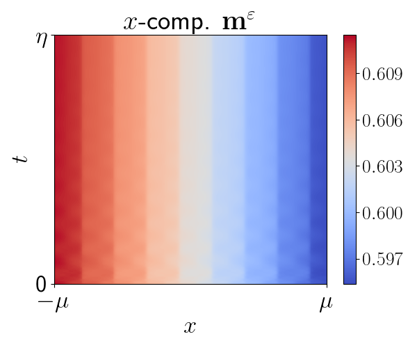
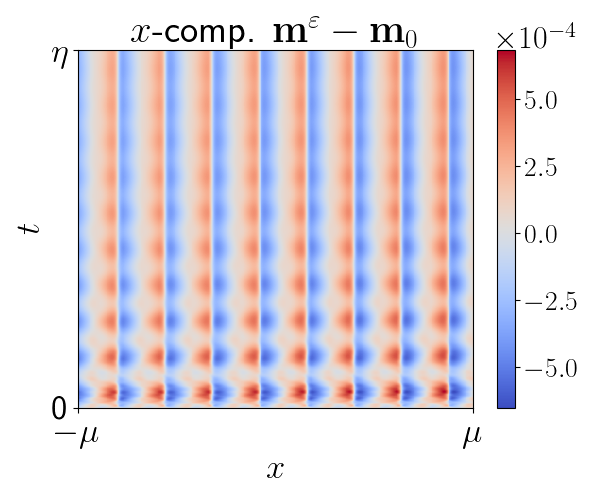
To create a better understanding of the problem, Fig. 1 shows the -component of the solution to an example problem in time and space as well as the difference between and the solution to the corresponding homogenized equation, . One can observe that oscillates in both time and space initially, but as increases the temporal oscillations are damped away and only the spatial ones remain. The oscillations have significantly smaller magnitude than the solution and appear to have zero average.
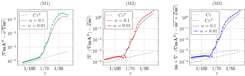
We then consider the approximation errors for the three models (M1) - (M3) and compare the observed behavior with the theoretical bound according to Theorem 5.1,
| (72) |
where and . In Fig. 2, the approximation errors for varying is shown. In Fig. 2(a), the damping constant is set to and in Fig. 2(b) we have . For all three models, the errors initially decrease rapidly with . In this regime, the error appears to be dominated by the term in 72. For smaller , the errors are proportional to . Note that this is smaller than the convergence rate of suggested by 72. In (M1) the error is somewhat lower than for (M2) and (M3). The latter two models result in very similar error behavior.
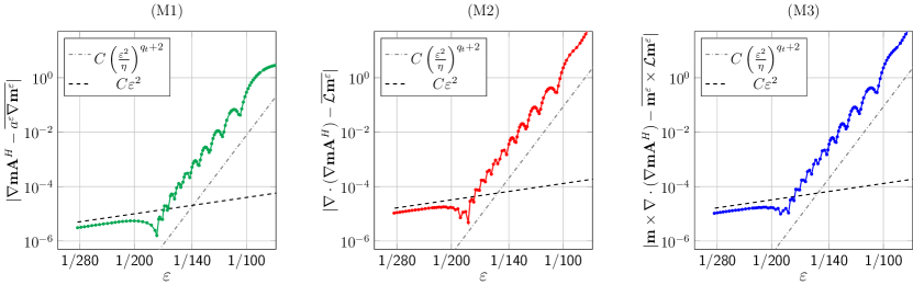
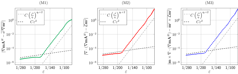
When comparing Fig. 2(a) and Fig. 2(b), one can moreover observe that choosing a lower damping parameter results in more oscillatory errors. However, the overall error behavior is very similar for both -values. This is a property that holds for all the examples considered here. We therefore choose to show plots for higher values of in several of the subsequent examples to reduce oscillations and make it easier to distinguish the different curves.
Next, we consider the influence of the kernel parameters and on the error decay. As shown in Figure 3, the choice of does not influence the error behavior, while different values of result in different slopes of the initial error decay. This again shows that the error from time averaging initially dominates in Figure 2 and Figure 3. In particular, it is proportional to until it reaches the threshold. This is slightly better than as given in Theorem 5.1.
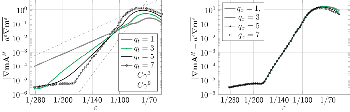
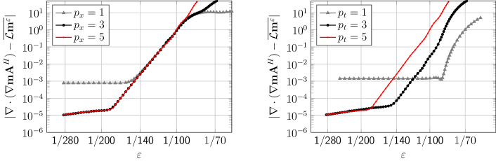
We continue by examining the influence of the parameters and and the contribution of the terms and to the error. As shown in Fig. 4, we find that low choices of both and result in a constant error for low , corresponding to or , respectively. For larger and , these terms are presumably smaller than , in the range considered. One can furthermore observe that the choice of does not seem to influence the error otherwise, while the initial convergence happens at different -values when varying .
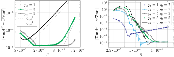
Finally, we investigate the influence of the choice of box sizes and on the error given a fixed value . In Fig. 5, it is shown that when increasing from a small value, there is some initial decrease in the error due to the reduction in before it takes a constant value, due to the fact that the other terms in 72 dominate. At some point, depending on , the error starts increasing again since the term starts dominating the error. When varying , we have a similar behavior. However, increasing results in a much larger initial error reduction, given that is chosen large enough. The slopes of this decrease depend on . Once is larger than a certain threshold, the error takes a constant value. When , the error only decreases initially and then starts increasing again due to the term .
Overall, we can conclude that for the 1D example problem, the error is considerably more affected by temporal than spatial averaging. The estimate in Theorem 5.1 matches conceptually well with the observed behavior but is slightly too pessimistic.
6.2 Two-dimensional examples
We here consider a periodic problem where the material coefficient is chosen to be
Solving the cell problem 7 numerically, the corresponding homogenized coefficient is computed to be
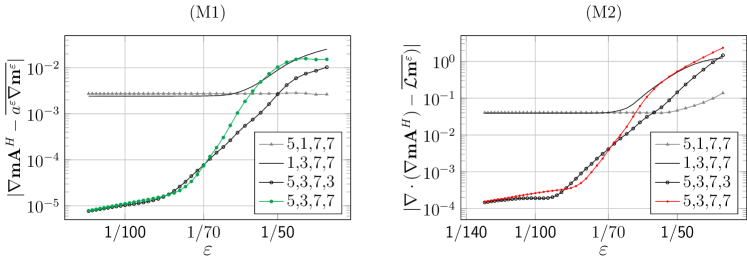
a full matrix with two different diagonal elements. The upscaling errors when varying in (M1), (M2) and (M3) for an example problem with this material coefficient is shown in Figure 6.
One can observe a similar behavior as for the 1D problem. However, note that the error in (M1) is considerably lower than for (M2) and (M3) in this example. In (M1) and (M2), we again observe convergence proportional to for low values of instead of as suggested by Theorem 5.1. However, the error in (M3) with low damping, , decays only proportionally to rather than . We suspect that this is related to the term in the analysis of the error in (M3), 66, the term taking the interaction of fast oscillations in time with each other into account. With higher , the temporal oscillations get damped away faster and we do not observe that behavior.
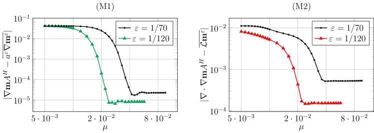
Apart from this observation for low , the errors in (M2) and (M3) behave very similar when varying the parameters in the model. We therefore focus on comparing (M1) and (M2) in the following. The influence of the kernel parameters is similar to the 1D problem. As shown in Fig. 7, choosing low or results in constant error when decreasing , corresponding to or , respectively. The parameter determines the speed of the initial decay. However, in contrast to the 1D case it is harder to specifically determine the slopes in this example.
In Figure 8, the error in (M1) and (M2) when varying is shown for two different values of , similar to Figure 5, right, in the 1D case. When choosing low , the errors are high but decrease rapidly as increases. From the error stays at a constant level.
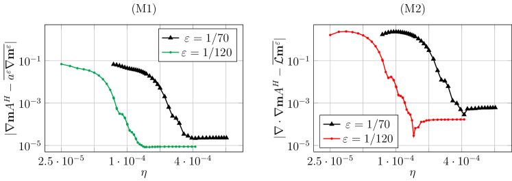
Finally, we investigate the influence of as shown in Fig. 9. We can observe rapidly decreasing errors until , then the errors are almost constant. In contrast to the 1D case, shown in Figure 5, left, the choice of has a significant impact on the error in this example. In particular, in (M1) the magnitude of the error is determined by and equally. In case of (M2), still has a somewhat larger impact than .
Acknowledgments
Support by the Swedish Research Council under grant no 2017-04579 is gratefully acknowledged.
References
- [1] A. Abdulle, E. Weinan, B. Engquist, and E. Vanden-Eijnden, The Heterogeneous Multiscale Method, Acta Numerica, 21 (2012), pp. 1–87.
- [2] F. Alouges, A. De Bouard, B. Merlet, and L. Nicolas, Stochastic homogenization of the Landau-Lifshitz-Gilbert equation, Stochastics and Partial Differential Equations: Analysis and Computations, (2021), pp. 1–30.
- [3] D. Arjmand, S. Engblom, and G. Kreiss, Temporal Upscaling in Micromagnetism via Heterogeneous Multiscale Methods, J. Comput. Appl. Math., 345 (2019), pp. 99–113.
- [4] D. Arjmand, G. Kreiss, and M. Poluektov, Atomistic-continuum multiscale modeling of magnetization dynamics at non-zero temperature, Adv. Comput. Math, 44 (2018), pp. 1119–1151.
- [5] D. Arjmand and O. Runborg, Analysis of heterogeneous multiscale methods for long time wave propagation problems, Multiscale Modeling & Simulation, 12 (2014), pp. 1135–1166.
- [6] D. Arjmand and O. Runborg, A time dependent approach for removing the cell boundary error in elliptic homogenization problems, Journal of Computational Physics, 314 (2016), pp. 206–227.
- [7] A. Bensoussan, J. Lions, and G. Papanicolaou, Asymptotic analysis for periodic structures, North-holland, 1978.
- [8] C. Choquet, M. Moumni, and M. Tilioua, Homogenization of the Landau-Lifshitz-Gilbert equation in a contrasted composite medium, Discrete & Continuous Dynamical Systems-S, 11 (2018), p. 35.
- [9] D. Cioranescu and P. Donato, An introduction to homogenization, Oxford University Press, 1999.
- [10] B. Engquist, H. Holst, and O. Runborg, Multi-scale methods for wave propagation in heterogeneous media, arXiv preprint arXiv:0911.2638, (2009).
- [11] B. Engquist, H. Holst, and O. Runborg, Analysis of HMM for one dimensional wave propagation problems over long time, arXiv preprint arXiv:1111.2541, (2011).
- [12] B. Engquist and Y.-H. Tsai, Heterogeneous multiscale methods for stiff ordinary differential equations, Mathematics of computation, 74 (2005), pp. 1707–1742.
- [13] K. Hamdache, Homogenization of layered ferromagnetic media, preprint, 495 (2002).
- [14] I. G. Kevrekidis, C. W. Gear, J. Hyman, P. G. Kevekidis, and O. Runborg, Equation-free, coarse-grained multiscale computation: Enabling microscopic simulators to perform system-level tasks., Comm. Math. Sci., (2003), pp. 715–762.
- [15] M. G. Krein and M. A. Ruthman, Linear operators that leave invariant a cone in a Banach space, Usp. Mat. Nauk., (1948).
- [16] L. Landau and E. Lifshitz, On the theory of dispersion of magnetic permeability in ferromagnetic bodies, Phys. Z. Sowjet., 8 (1935), pp. 153–168.
- [17] L. Leitenmaier and O. Runborg, Homogenization of the Landau-Lifshitz equation, arXiv preprint arXiv:2012.12567, (2020).
- [18] M. J. D. Powell et al., Approximation theory and methods, Cambridge University Press, 1981.
- [19] K. Santugini-Repiquet, Homogenization of ferromagnetic multilayers in the presence of surface energies, ESAIM: Control, Optimisation and Calculus of Variations, 13 (2007), pp. 305–330.
- [20] E. Weinan, B. Engquist, et al., The Heterognous Multiscale Methods, Communications in Mathematical Sciences, 1 (2003), pp. 87–132.
- [21] E. Weinan, B. Engquist, X. Li, W. Ren, and E. Vanden-Eijnden, Heterogeneous Multiscale Methods: a review, Communications in computational physics, 2 (2007), pp. 367–450.