h KA-TP-07-2021
One-loop Corrections to the Higgs Boson Invisible Decay in the Dark Doublet Phase of the N2HDM

Abstract

The Higgs invisible decay width may soon become a powerful tool to probe extensions of the Standard Model with dark matter candidates at the Large Hadron Collider. In this work, we calculate the next-to-leading order (NLO) electroweak corrections to the 125 GeV Higgs decay width into two dark matter particles. The model is the next-to-minimal 2-Higgs-doublet model (N2HDM) in the dark doublet phase, that is, only one doublet and the singlet acquire vacuum expectation values. We show that the present measurement of the Higgs invisible branching ratio, BR$(H\to$ invisible $<0.11$), does not lead to constraints on the parameter space of the model at leading order. This is due to the very precise measurements of the Higgs couplings but could change in the near future. Furthermore, if NLO corrections are required not to be unphysically large, no limits on the parameter space can be extracted from the NLO results.

1 Introduction

Ever since the Higgs boson was discovered at the Large Hadron Collider (LHC) by the ATLAS [1] and CMS [2] collaborations, the measurement of the Higgs couplings to the remaining Standard Model (SM) particles became a powerful tool in constraining the parameter space of extensions of the SM. Another important ingredient when building extensions of the SM with dark matter (DM) candidates is the measurement of the invisible Higgs branching ratio. Very recently, a new result by the ATLAS collaboration combining 139 fb^-1 of data at $\sqrt{s}=13$ TeV with the results obtained at $\sqrt{s}=7$ and $8$ TeV was published. The observed upper limit on the SM-like Higgs ($H_{\text{SM}}$) to invisibles branching ratio (BR) is 0.11 [3], which is an improvement from the previous result with an invisible BR above 0.2. The results of the Higgs coupling measurements together with those of the invisible Higgs decay are our best tools at colliders to constrain extensions of the scalar sector of the SM with DM candidates.

We will focus on a specific phase of the next-to-minimal 2-Higgs-doublet model (N2HDM) with a scalar sector consisting of two complex doublets and one real singlet. Only one of the doublets and the singlet acquire vacuum expectation values (VEVs) and we end up with two possible DM candidates. This particular phase of the N2HDM is known as the dark doublet phase (DDP). The different phases of the N2HDM are described in detail in [4].

Our analysis will be performed by first imposing the most relevant theoretical and experimental constraints on the model. We then calculate the next-to-leading (NLO) electroweak corrections to the invisible decay of the SM-like Higgs boson, that is, the Higgs decaying into two DM candidates. The results will be presented for all allowed parameter space points, which will enable us to understand if NLO corrections can help to constrain the parameter space of the N2HDM. The NLO BR of Higgs to invisibles could be larger than the experimentally measured value for some regions of the parameter space.

As shown in a recent work [4], the constraints coming from the Higgs couplings to fermions and gauge bosons are enough to indirectly constrain the BR of the Higgs decay into invisibles to be below 0.1 in the N2HDM (DDP phase). So until recently, the Higgs BR to invisible was not a meaningful experimental result to constrain the parameter space. However, the new measurement by ATLAS, reaching now 0.11, is exactly at the frontier between the indirect bound coming from Higgs couplings and the direct one coming from the invisibles Higgs BR. So it is extremely timely to calculate the electroweak (EW) NLO corrections to the Higgs invisible BR.

The outline of the paper is as follows. In section 2, we will introduce the DDP phase of the N2HDM together with our notation. Section 3 is dedicated to the description of the different renormalization schemes used in this work. In section 4 we discuss the expressions of the Higgs invisible decay at leading order (LO) and at NLO. In section 5, the results are presented and discussed. Our conclusions are collected in section 6. There are two appendices where we discuss details of the renormalization procedure.

2 Model

We start this section by describing the dark doublet phase of the N2HDM [5, 6, 7, 8, 4]. The Higgs sector of the N2HDM is composed of two $SU(2)_{L}$ doublet fields with hypercharge Y=1, $\Phi_{i}$ ($i=1,2$), and the real $SU(2)_{L}$ singlet field $\Phi_{S}$ with hypercharge Y=0. Two discrete $\mathbb{Z}_{2}$ symmetries, $\mathbb{Z}^{(1)}_{2}$ and $\mathbb{Z}^{(2)}_{2}$, are imposed on the model. Under these symmetries, each scalar field is transformed as

$$\mathbb{Z}^{(1)}_{2}: \quad\Phi_{1}\rightarrow\Phi_{1},\quad\Phi_{2}\rightarrow-\Phi_{2},\quad\Phi_{S}\rightarrow\Phi_{S}\,,$$ (1)

$$\mathbb{Z}^{(2)}_{2}: \quad\Phi_{1}\rightarrow\Phi_{1},\quad\Phi_{2}\rightarrow\Phi_{2},\quad\Phi_{S}\rightarrow-\Phi_{S}\,.$$ (2)

We require the $\mathbb{Z}_{2}$ symmetries to be exact, meaning that no soft breaking terms are introduced, and therefore the Higgs potential of the N2HDM is given by [5, 6, 7, 8, 4]

$$V= \enspace m_{11}^{2}\Phi_{1}^{\dagger}\Phi_{1}+m_{22}^{2}\Phi_{2}^{\dagger}\Phi_{2}+\dfrac{\lambda_{1}}{2}\left(\Phi_{1}^{\dagger}\Phi_{1}\right)^{2}+\dfrac{\lambda_{2}}{2}\left(\Phi_{2}^{\dagger}\Phi_{2}\right)^{2}$$

$$+\enspace\lambda_{3}\Phi_{1}^{\dagger}\Phi_{1}\Phi_{2}^{\dagger}\Phi_{2}+\lambda_{4}\Phi_{1}^{\dagger}\Phi_{2}\Phi_{2}^{\dagger}\Phi_{1}+\dfrac{\lambda_{5}}{2}\left[\left(\Phi_{1}^{\dagger}\Phi_{2}\right)^{2}+\text{h.c.}\right]$$ (3)

$$+\enspace\dfrac{1}{2}m_{s}^{2}\Phi_{S}^{2}+\dfrac{\lambda_{6}}{8}\Phi_{S}^{4}+\dfrac{\lambda_{7}}{2}\Phi_{1}^{\dagger}\Phi_{1}\Phi_{S}^{2}+\dfrac{\lambda_{8}}{2}\Phi_{2}^{\dagger}\Phi_{2}\Phi_{S}^{2}\,,$$

where all parameters can be set real by rephasing $\Phi_{1}$ or $\Phi_{2}$. In the N2HDM, there are four different minima, which break the $SU(2)\times U(1)_{Y}$ symmetry into $U_{\rm EM}(1)$, depending on the vacuum expectation values for the doublet fields and the singlet field, i.e. $\left<\Phi_{1}\right>,\ \left<\Phi_{2}\right>$ and $\left<\Phi_{S}\right>$, respectively. The possible patterns are

broken phase (BP): $$\left<\Phi_{1}\right>\neq 0\,,\left<\Phi_{2}\right>\neq 0\,,\left<\Phi_{S}\right>\neq 0\,,$$ (4)

dark doublet phase (DDP): $$\left<\Phi_{1}\right>\neq 0\,,\left<\Phi_{2}\right>=0\,,\left<\Phi_{S}\right>\neq 0\,,$$ (5)

dark singlet phase (DSP): $$\left<\Phi_{1}\right>\neq 0\,,\left<\Phi_{2}\right>\neq 0\,,\left<\Phi_{S}\right>=0\,,$$ (6)

full dark phase (FDP): $$\left<\Phi_{1}\right>\neq 0\,,\left<\Phi_{2}\right>=0\,,\left<\Phi_{S}\right>=0\,.$$ (7)

In this study, we focus on the DDP, where $\mathbb{Z}^{(1)}_{2}$ remains unbroken while $\mathbb{Z}^{(2)}_{2}$ is spontaneously broken. Hence, this phase corresponds to an extension of the inert doublet model (IDM) [9] by the additional singlet field. The other phases are discussed in Refs. [5, 6, 7, 8, 4].

In the DDP, the components of the Higgs fields can be parameterized as

$$\Phi_{1}=\begin{pmatrix}G^{+}\\ \dfrac{1}{\sqrt{2}}\left(v+\rho_{1}+i\,G^{0}\right)\end{pmatrix},\quad\Phi_{2}=\begin{pmatrix}H^{+}_{D}\\ \dfrac{1}{\sqrt{2}}\left(H_{D}+i\,A_{D}\right)\end{pmatrix},\quad\Phi_{S}=v_{s}+\rho_{s}\,,$$ (8)

where $v=246$ GeV is the electroweak VEV and $v_{S}$ is the VEV of the singlet field. The doublet field $\Phi_{1}$ corresponds the SM Higgs doublet, which contains the Nambu-Goldstone bosons $G^{+}$ and $G^{0}$. Due to the unbroken $\mathbb{Z}^{(1)}_{2}$ symmetry, the four dark scalars, $H_{D},A_{D}$ and $H^{\pm}_{D}$ do not mix, i.e., they are physical states. The lightest neutral dark scalar, which can be either $H_{D}$ or $A_{D}$, is the DM candidate. On the other hand, the two CP-even Higgs fields $\rho_{1}$ and $\rho_{S}$ mix with each other. Together with the CP-even dark scalar $H_{D}$, the mass eigenstates for the CP-even Higgs bosons can be expressed through a rotation matrix with the mixing angle $\alpha$ as,

$$\left(\begin{array}[]{c}H_{1}\\ H_{2}\\ H_{D}\end{array}\right)=\left(\begin{array}[]{ccc}c_{\alpha}&0&s_{\alpha}\\ -s_{\alpha}&0&c_{\alpha}\\ 0&1&0\end{array}\right)\left(\begin{array}[]{c}\rho_{1}\\ H_{D}\\ \rho_{S}\end{array}\right),$$ (18)

where by convention, we take $m_{H_{1}}<m_{H_{2}}$, and where we have introduced the short-hand notations $c_{\alpha}\equiv\cos\alpha$ and $s_{\alpha}\equiv\sin\alpha$. Either $H_{1}$ or $H_{2}$ can be identified as the SM-like Higgs boson ($H_{\text{SM}}$) with a mass of 125 GeV. For later convenience, we define the rotation matrix as $R$, so that Eq. (18) can be rewritten by $H_{i}=R_{ij}\rho_{j}$ ($i,j=1,2,3$), defining $\rho_{2}=H_{D}$ and $\rho_{3}=\rho_{S}$.

The masses of the physical states can be written as

$$m^{2}_{H_{1}} =v^{2}\cos^{2}\alpha\,\lambda_{1}+v_{s}^{2}\sin^{2}\alpha\,\lambda_{6}+2vv_{s}\sin\alpha\,\cos\alpha\,\lambda_{7}\,,$$ (19)

$$m^{2}_{H_{2}} =v^{2}\sin^{2}\alpha\,\lambda_{1}+v_{s}^{2}\cos^{2}\alpha\,\lambda_{6}-2vv_{s}\sin\alpha\,\cos\alpha\,\lambda_{7}\,,$$ (20)

$$m^{2}_{H_{D}} =\dfrac{1}{2}(2m_{22}^{2}+v^{2}(\lambda_{3}+\lambda_{4}+\lambda_{5})+v_{s}^{2}\lambda_{8})\,,$$ (21)

$$m^{2}_{A_{D}} =\dfrac{1}{2}(2m_{22}^{2}+v^{2}(\lambda_{3}+\lambda_{4}-\lambda_{5})+v_{s}^{2}\lambda_{8})\,,$$ (22)

$$m^{2}_{H_{D}^{\pm}} =\dfrac{1}{2}(2m_{22}^{2}+v^{2}\lambda_{3}+v_{s}^{2}\lambda_{8})\,.$$ (23)

Using these mass formulae together with the mixing angle $\alpha$ and the stationary conditions for $\Phi_{1}$ and $\Phi_{S}$, i.e.,

$$\left<\partial V/\partial\Phi_{1}\right>\equiv T_{\Phi}/v=0\quad\mbox{and}\quad\left<\partial V/\partial\Phi_{S}\right>\equiv T_{S}/v_{S}=0\;,$$ (24)

the original parameters of the potential can be replaced by a new set to be used as input. Together with the electroweak and singlet VEVs, we choose as our input the following 13 parameters,

$$v\,,\enspace v_{s}\,,\enspace m_{H_{1}}\,,\enspace m_{H_{2}}\,,\enspace m_{H_{D}}\,,\enspace m_{A_{D}}\,,\enspace m_{H_{D}^{\pm}}\,,\enspace\alpha\,,\enspace m_{22}^{2}\,,\enspace T_{\Phi}\,,\enspace T_{S}\,,\enspace\lambda_{2}\,,\enspace\lambda_{8}\,.$$ (25)

We assign $\mathbb{Z}^{(1)}_{2}$-even and $\mathbb{Z}^{(2)}_{2}$-even parity to the remaining SM fields and consequently only the Higgs doublet $\Phi_{1}$ has Yukawa interactions. This in turn means that the Yukawa couplings are just the SM ones and that the dark scalars do not couple to the SM fermions. On the other hand, due to the kinetic term for $\Phi_{2}$, dark scalar-dark scalar-gauge boson type of vertices are allowed while the dark scalar-gauge boson-gauge boson type of vertices are forbidden by the $\mathbb{Z}^{(1)}_{2}$ symmetry. The Feynman rules for the vertices including two dark scalars and a gauge boson are written in Ref [4]. In particular, the trilinear scalar couplings that are relevant for the calculation of the invisible decay of the Higgs boson are given by ($i=1,2$)

$$\lambda_{H_{i}H_{D}H_{D}}=-\frac{1}{v}\big{[}2(m_{H_{D}}^{2}-m_{22}^{2})R_{i1}+\lambda_{8}v_{S}(vR_{i3}-v_{S}R_{i1})\big{]}\;.$$ (26)

We note that in the case of $\cos\alpha=1$ and $\lambda_{8}=0$ the expression of $\lambda_{H_{i}H_{D}H_{D}}$ is exactly the IDM one. The other trilinear scalar couplings are also given in Ref. [4].

3 Renormalization

In this section, we discuss the renormalization scheme used in the calculation of the one-loop corrections to the Higgs boson $H_{i}$ $(i=1,2)$ decay into a pair of DM particles, which we assume to be $H_{D}$, unless otherwise stated, $H_{i}\to H_{D}H_{D}$. Thus, this section focuses on the renormalization of the scalar and gauge sectors. The renormalization of the fermion sector as well as any treatment of infrared divergence is not necessary for this particular process.

We perform the renormalization of the Higgs sector in the DDP of the N2HDM according to the procedure presented in Ref. [10] for the 2HDM and in Ref. [11] for the broken phase of the N2HDM. Although most of the parameters in the Higgs sector of the DDP are common with those of the broken phase, we describe the renormalization of all parameters in order to make the paper self-contained.

3.1 Gauge sector

The renormalization of all parameters and fields in the gauge sector is done using the on-shell (OS) scheme following Ref. [12]. As the three independent parameters in this sector, we choose the masses of weak gauge bosons and the electric charge, i.e., $m_{W}$, $m_{Z}$, and $e$, respectively. These parameters are shifted as

$$m_{V}^{2} \to m_{V}^{2}+\delta m_{V}^{2}\quad(V=W,Z)\;,$$ (27)

$$e \to(1+\delta Z_{e})e\;.$$ (28)

Moreover, the bare fields for the gauge bosons in the mass basis are replaced by the renormalized ones as

$$W^{\pm} \to(1+\frac{1}{2}\delta Z_{WW})W^{\pm}\,,$$

$$\begin{pmatrix}Z\\ \gamma\end{pmatrix} \to\begin{pmatrix}1+\frac{1}{2}\delta Z_{ZZ}&\frac{1}{2}\delta Z_{Z\gamma}\\ \frac{1}{2}\delta Z_{\gamma Z}&1+\frac{1}{2}\delta Z_{\gamma\gamma}\end{pmatrix}\begin{pmatrix}Z\\ \gamma\end{pmatrix}\,.$$ (29)

The OS conditions for these gauge fields are defined as

$$\delta m_{W}^{2}=\mbox{Re}\Sigma^{\text{tad},T}_{WW}(m_{W}^{2})\quad\mbox{and}\quad\delta m_{Z}^{2}=\mbox{Re}\Sigma^{\text{tad},T}_{ZZ}(m_{Z}^{2})\;,$$ (30)

$$\delta Z_{WW} = -\mbox{Re}\left.\frac{\partial\Sigma^{T}_{WW}(p^{2})}{\partial p^{2}}\right|_{p^{2}=m_{W}^{2}}\,,$$ (31)

$$\left(\begin{array}[]{cc}\delta Z_{ZZ}&\delta Z_{Z\gamma}\\ \delta Z_{\gamma Z}&\delta Z_{\gamma\gamma}\end{array}\right) = \left(\begin{array}[]{cc}-\mbox{Re}\left.\frac{\partial\Sigma^{T}_{ZZ}(p^{2})}{\partial p^{2}}\right|_{p^{2}=m_{Z}^{2}}&2\mbox{Re}\frac{\Sigma^{T}_{Z\gamma}(0)}{m_{Z}^{2}}\\ -2\mbox{Re}\frac{\Sigma^{T}_{Z\gamma}(m_{Z}^{2})}{m_{Z}^{2}}&-\left.\frac{\partial\Sigma^{T}_{\gamma\gamma}(p^{2})}{\partial p^{2}}\right|_{p^{2}=0}\end{array}\right)\;,$$ (36)

where $\Sigma^{\text{tad},T}_{WW}$ and $\Sigma^{\text{tad},T}_{ZZ}$ denote the transverse part of the self-energies of the $W$ and $Z$ bosons. These contain the tadpole contributions due to our renormalization scheme choice. No “tad” superscript means that there is no contribution from the tadpole diagrams. The different tadpole schemes will be described below. The counterterm for the electric charge is determined from $\gamma e\bar{e}$ in the Thomson limit and can be expressed as a function of the self-energies as

$$\delta Z_{e}^{\alpha(0)} = \frac{1}{2}\left.\frac{\partial\Sigma^{T}_{\gamma\gamma}(k^{2})}{\partial k^{2}}\right|_{k^{2}=0}+\frac{s_{W}}{c_{W}}\frac{\Sigma_{\gamma Z}^{T}(0)}{m_{Z}^{2}}\;.$$ (37)

This counterterm contains large logarithmic corrections arising from the small fermion masses, $\log m^{2}_{f}\leavevmode\nobreak\ (f\neq t)$. We use the “$G_{\mu}$ scheme” [13] in order to improve the perturbative behaviour. In this scheme, a large universal part of the ${\cal O}(\alpha)$ corrections is absorbed in the leading order decay width by deriving the electromagnetic coupling constant $\alpha=e^{2}/(4\pi)$ from the Fermi constant, $G_{\mu}$, as

$$\alpha_{G_{\mu}}=\frac{\sqrt{2}G_{\mu}m_{W}^{2}}{\pi}\left(1-\frac{m_{W}^{2}}{m_{Z}^{2}}\right)\;.$$ (38)

This allows us to take into account the running of the electromagnetic coupling constant $\alpha(Q^{2})$, from $Q^{2}=0$ to the electroweak scale. In order to avoid double counting, the corrections that are absorbed in the LO decay width by using $\alpha_{G_{\mu}}$ have to be subtracted from the explicit ${\cal O}(\alpha)$ corrections. This is achieved by subtracting the weak corrections to the muon decay, $\Delta r$ [12, 14], from the corrections in the $\alpha(0)$ scheme. Hence, we redefine the charge renormalization constant as

$$\delta Z_{e}|_{G_{\mu}}=\delta Z_{e}|_{\alpha(0)}-\frac{1}{2}(\Delta r)_{\text{1-loop}}\;,$$ (39)

where $(\Delta r)_{\text{1-loop}}$ is the one-loop expression for $\Delta r$ given by [12]

$$(\Delta r)_{\text{1-loop}} = \left.\frac{\partial\Sigma^{T}_{\gamma\gamma}(k^{2})}{\partial k^{2}}\right|_{k^{2}=0}-\frac{c_{W}^{2}}{s_{W}^{2}}\left(\frac{\Sigma_{ZZ}^{T}(m_{Z}^{2})}{m_{Z}^{2}}-\frac{\Sigma_{WW}^{T}(m_{W}^{2})}{m_{W}^{2}}\right)+\frac{\Sigma_{WW}^{T}(0)-\Sigma_{WW}^{T}(m_{W}^{2})}{m_{W}^{2}}$$ (40)

$$-2\frac{c_{W}}{s_{W}}\frac{\Sigma_{\gamma Z}^{T}(0)}{m_{Z}^{2}}+\frac{\alpha}{4\pi s_{W}^{2}}\left(6+\frac{7-4s_{W}^{2}}{2s_{W}^{2}}\log c_{W}^{2}\right)\;.$$

Note that through the redefinition Eq. (39), the first term of $\delta Z_{e}^{\alpha(0)}$ in Eq. (37), which contains the large logarithmic corrections from the light fermion loops, cancels against the corresponding term in $(\Delta r)_{\text{1-loop}}$. The counterterms for the other EW parameters can be expressed in terms of those presented above. For example, the $SU(2)_{L}$ gauge coupling, $g$, is replaced by the tree level relation $g=em_{Z}/\sqrt{m_{Z}^{2}-m_{W}^{2}}$. Thus, the counterterm is given by

$$\frac{\delta g}{g}=\delta{Z_{e}}-\frac{1}{2(1-m^{2}_{Z}/m^{2}_{W})}\left(\frac{\delta m_{W}^{2}}{m_{W}^{2}}-\frac{\delta m_{Z}^{2}}{m_{Z}^{2}}\right)\,.$$ (41)

3.2 Higgs sector

In the Higgs sector, we have a total of 13 free parameters, given in Eq. (25), considering the two tadpoles $T_{\Phi}$ and $T_{S}$. We have to renormalize the scalar fields in the mass basis, $H_{1}$, $H_{2}$, $H_{D}$, $A_{D}$ and $H^{\pm}_{D}$. The counterterms are introduced via the shift of the input parameters, i.e, the masses of the scalar bosons, the mixing angle $\alpha$ of the CP-even Higgs bosons and the remaining original potential parameters that appear in the vertices of the processes under study, $\lambda_{8}$ and $m_{22}^{2}$,

$$m_{\Phi}^{2}\to m_{\Phi}^{2}+\delta m_{\Phi}^{2}\,,\quad\alpha\to\alpha+\delta\alpha\,,$$

$$m_{22}^{2}\to m_{22}^{2}+\delta m_{22}^{2}\,,\quad\lambda_{8}\to\lambda_{8}+\delta\lambda_{8}\,,$$ (42)

where $\Phi$ denotes $H_{1},\ H_{2},\ H_{D},\ A_{D},$ and $H^{\pm}_{D}$. There is no need to renormalize $\lambda_{2}$ for this particular process. Apart from the tadpoles, the remaining two parameters are the VEVs. The electroweak VEV $v$ is fixed by the $W$ mass and the renormalization of $v_{S}$ will be discussed later.

The tadpole renormalization can be performed in different ways and we will discuss two approaches. These are designated by Standard Tadpole Scheme (STS) and Alternative Tadpole Scheme (ATS). The latter was originally proposed by Fleischer and Jegerlehner, in Ref. [15], for the SM. The ATS was also discussed in detail for the CP-conserving 2HDM in Ref. [10] and for the broken phase of the N2HDM in Ref. [11]. We will just briefly review the two schemes for completeness.

In the STS, the tree level tadpoles are replaced by

$$T_{X}\to T_{X}+\delta T_{X}\quad(X=\Phi,S)\,,$$ (43)

and are chosen as the renormalization parameters. On the other hand, in the ATS, the VEVs are the renormalization parameters and are shifted as

$$v\to v+\delta v\,,\quad v_{S}\to v_{S}+\delta v_{S}\,.$$ (44)

We use the ATS, which will now be explained in more detail. The reason to use this scheme is that, as shown by Fleischer and Jegerlehner, all renormalized parameters are gauge independent except for the wave function renormalization constants (or any parameter that depends on the wave function renormalizaton constants as is the case of the angle $\alpha$ in particular schemes).

Before moving to the discussion of the tadpole renormalization, we define the wave function renormalization constants of the scalar fields. The bare fields are replaced by the renormalized ones through

$$\left(\begin{array}[]{c}H_{1}\\ H_{2}\\ H_{D}\end{array}\right)\to\left(\begin{array}[]{ccc}1+\frac{1}{2}\delta Z_{H_{1}H_{1}}&\frac{1}{2}\delta Z_{H_{1}H_{2}}&0\\ \frac{1}{2}\delta Z_{H_{2}H_{1}}&1+\frac{1}{2}\delta Z_{H_{2}H_{2}}&0\\ 0&0&1+\frac{1}{2}\delta Z_{H_{D}H_{D}}\end{array}\right)\left(\begin{array}[]{c}H_{1}\\ H_{2}\\ H_{D}\end{array}\right)\,,$$ (54)

$$A_{D}\to A_{D}(1+\frac{1}{2}\delta Z_{A_{D}})\,,\quad H^{\pm}_{D}\to H^{\pm}_{D}(1+\frac{1}{2}\delta Z_{H^{\pm}_{D}})\,.$$ (55)

Note that, for Eq. (54), the exact $\mathbb{Z}^{(1)}_{2}$ symmetry ensures that the $(3$-$k)$ and $(k$-$3)$ components ($k=1,2$) are zero.

3.2.1 Tadpoles

In the ATS, the renormalized VEVs, which correspond to minima of the Higgs potential at loop-level, are regarded as the tree-level VEVs, namely, one imposes

$$v^{\rm bare} =v^{\rm ren}+\delta v\overset{\rm FJ}{=}v^{\rm tree}+\delta v\,,$$

$$v^{\rm bare}_{S} =v^{\rm ren}_{S}+\delta v_{S}\overset{\rm FJ}{=}v^{\rm tree}_{S}+\delta v_{S}\,.\quad$$ (56)

Using the tadpole conditions, one can derive expressions for $\delta v$ and $\delta v_{S}$,

$$T_{i}^{\rm bare}=T_{i}^{\rm tree}+f(\delta v,\delta v_{S})=T_{i}^{\rm loop}\quad(i=\Phi,S)\,,$$ (57)

where the first term, $T_{i}^{\rm tree}$, is zero from the stationary condition at the tree-level and the second term, $f(\delta v,\delta v_{S})$, denotes contributions from $\delta v$ and $\delta{v_{S}}$, which can be extracted by inserting Eq. (44) into the tree-level tadpole conditions. From Eq. (57) one obtains the following expressions for the VEV counterterms

$${\cal R}(\alpha)\left(\begin{array}[]{c}\delta v\\ \delta v_{S}\end{array}\right)=\,\left(\begin{array}[]{c}\frac{T_{H_{1}}^{\text{loop}}}{m^{2}_{H_{1}}}\\ \frac{T_{H_{2}}^{\text{loop}}}{m^{2}_{H_{2}}}\end{array}\right)\,,$$ (58)

where ${\cal R}(\alpha)$ denotes the $2\times 2$ non-diagonal part of $R$ (see Eq. (18)),

$${\cal R}_{11}={\cal R}_{22}=\cos\alpha\;,\quad{\cal R}_{12}=-{\cal R}_{21}=\sin\alpha\;,$$ (59)

and the one-loop tadpoles in the mass basis are given by $T_{H_{i}}^{\rm loop}=({\cal R}(\alpha))_{ij}T_{j}^{\rm loop}$ ($i,j=1,2$) with $T_{1}=T_{\Phi}$ and $T_{2}=T_{S}$. The left-hand side corresponds to the VEV counterterms $\delta v_{H_{1}}$ and $\delta v_{H_{2}}$ in the mass basis and the right-hand side coincides with the tadpole diagrams multiplied by the propagator for the Higgs bosons at zero momentum transfer, i.e. $T_{H_{i}}^{\rm loop}/m_{H_{i}}^{2}=(iT_{H_{i}}^{\rm loop})(-i/m_{H_{i}}^{2})$. Therefore, Eq. (58) shows that $\delta v_{H_{i}}$ can be regarded as the connected tadpole diagrams for $H_{i}$. Once the counterterms for the VEVs are fixed, the shift is performed in all VEV terms in the Lagrangian. Hence in the ATS, one needs to insert tadpole diagrams in all amplitudes for which the original vertices contain one of the VEVs in addition to the usual one-particle irreducible diagrams. This general consequence is shown by focusing on specific amplitudes in Ref. [10] for the 2HDM and in Ref. [11] for the N2HDM.

Another important feature of the ATS is that, because the renormalized VEV is identified with the tree level VEV, the VEVs still have to be renormalized. For the EW VEV, the renormalized parameter is given by

$$v^{\rm ren}=v^{\rm tree}=2\left.\frac{m_{W}}{g}\right|^{\rm tree}\,,$$ (60)

and the tree-level parameters $g$ and $m_{W}$ are shifted as

$$2\left.\frac{m_{W}}{g}\right|^{\rm tree} \to 2\left.\frac{m_{W}}{g}\right|^{\rm ren}+\frac{2m_{W}}{g}\left(\frac{\delta m_{W}^{2}}{2m_{W}^{2}}-\frac{\delta g}{g}\right)$$

$$\equiv 2\left.\frac{m_{W}}{g}\right|^{\rm ren}+\Delta v\,.$$ (61)

We have defined the shift of the tree level parameters related to the EW VEV as $\Delta v$, which has no relation with $\delta v$. The same discussion holds for the singlet VEV $v_{S}$. Once $v_{S}$ is related with some measurable quantity, a similar relation with Eq.(60) must exist, even if a physical process has to be used, and then $\Delta v_{S}$ has to be introduced.

3.2.2 Mass and Wave Function Renormalization

The counterterms for the masses and the wave function renormalization constants (WFRCs) are determined by imposing the on-shell conditions for each scalar field. This yields the mass counterterms

$$\delta m_{\Phi}^{2} =\Sigma^{\rm tad}_{\Phi\Phi}(m_{\Phi}^{2})\,,$$ (62)

and the WFRCs

$$\delta Z_{\Phi\Phi} =-\frac{\partial\Sigma^{\rm tad}_{\Phi\Phi}(p^{2})}{\partial p^{2}}\Big{|}_{p^{2}=m_{\Phi}^{2}}\,,$$ (63)

$$\delta Z_{H_{i}H_{j}} =2\frac{\Sigma^{\rm tad}_{H_{i}H_{j}}(m_{H_{j}}^{2})}{m_{H_{i}}^{2}-m_{H_{j}}^{2}}\quad(i=1,2,j\neq i)\,,$$ (64)

where, to reiterate, $\Sigma^{\rm tad}$ stands for the self-energy containing one particle irreducible (1PI) diagrams and tadpole contributions.

3.2.3 Mixing angle $\alpha$

The renormalization of the mixing angle, $\alpha$, requires special treatment since the gauge dependence of $\delta\alpha$ could result in a gauge-dependent physical process [16, 17, 18, 19, 20, 21, 22, 23, 24, 25, 26]. A gauge-independent amplitude can be obtained by starting with a gauge-independent definition of $\delta\alpha$. One possible solution to avoid this gauge dependence is to apply the ATS for the renormalization of the tadpoles and to make use of the pinch technique [27, 28], while keeping the on-shell renormalization for the mixing angle. This is the procedure that we adopt throughout this paper.

The expression for $\delta\alpha$ in the OS scheme can be derived by relating quantities in the gauge basis to the corresponding ones in the physical (mass) basis. This procedure is described in detail in [29, 30, 10]. Following [10] leads to the following expression for $\delta\alpha$ after adding the pinched terms,

$$\delta\alpha =\frac{1}{4}(\delta Z_{H_{1}H_{2}}-\delta Z_{H_{2}H_{1}})$$

$$+\frac{1}{2}\frac{1}{m_{H_{1}}^{2}-m_{H_{2}}^{2}}\left[\Sigma_{H_{1}H_{2}}(m_{H_{2}}^{2})+\Sigma_{H_{1}H_{2}}(m_{H_{1}}^{2})\right]\,,$$ (65)

where $\Sigma_{H_{1}H_{2}}$ stands for pinched contributions to the $H_{1}-H_{2}$ mixing self-energy, which remove the gauge-dependent part coming from the first two terms. They can be extracted from the expressions obtained for the broken phase of the N2HDM (see [11]) as

$$\Sigma_{H_{1}H_{2}}(q^{2})=-\frac{g^{2}}{32\pi^{2}c_{W}^{2}}c_{\alpha}s_{\alpha}\left(q^{2}-\frac{m_{H_{1}}^{2}+m_{H_{2}}^{2}}{2}\right)$$

$$\times\left\{B_{0}(q^{2};m_{Z}^{2},m_{Z}^{2})+2c_{W}^{2}B_{0}(q^{2};m_{W}^{2},m_{W}^{2})\right\}\,.$$ (66)

The expression was obtained with the replacement $(\beta-\alpha_{1},\alpha_{2},\alpha_{3})\to(\alpha,0,0)$ and the fact that the $(A_{D},Z)$ and $(H_{D}^{\pm},W)$ loop contributions do not appear in our calculation due to the existence of an exact $\mathbb{Z}^{(1)}_{2}$ symmetry.

3.2.4 Counterterms for ${\lambda_{8}}$ and $m_{22}^{2}$

The counterterms for the quartic coupling ${\delta\lambda_{8}}$ and the invariant mass for the dark scalars ${\delta m_{22}^{2}}$ cannot be renormalized using OS conditions for the Higgs states. Hence we will renormalize these parameters using three different schemes: the $\overline{\rm MS}$ scheme, a process-dependent scheme and one derivation of the latter that consists of taking the external momenta to be zero instead of taking them on-mass-shell.

In the $\overline{\rm MS}$ scheme, the analytic expressions for the counterterms can be extracted from the beta functions at one-loop, yielding

$$\delta\lambda_{8}=\frac{1}{32\pi^{2}}\beta_{\lambda_{8}}^{(1)}\Delta_{\rm div}\,,\ \ \ \delta m_{22}^{2}=\frac{1}{32\pi^{2}}\beta_{m_{22}^{2}}^{(1)}\Delta_{\rm div}\,,$$ (67)

where $\Delta_{\rm div}$ denotes the UV-divergent part, i.e., $\Delta_{\rm div}=1/\epsilon-\gamma_{E}+\log(4\pi)$. $\gamma_{E}$ is the Euler-Mascheroni constant and $1/\epsilon$ is the UV pole in dimensional regularisation. The beta functions are given in terms of the original potential parameters by

$$\beta_{\lambda_{8}}^{(1)} =2\lambda_{4}\lambda_{7}+4\lambda_{3}\lambda_{7}+\frac{1}{10}\lambda_{8}\Big{(}30\lambda_{6}+40\lambda_{8}-45g_{2}^{2}+60\lambda_{2}-9C^{2}g_{1}^{2}\Big{)}\,,$$ (68)

$$\beta_{m^{2}_{22}}^{(1)} =2\lambda_{4}m^{2}_{11}+4\lambda_{3}m^{2}_{11}+6\lambda_{2}m^{2}_{22}-\frac{9}{10}C^{2}g_{1}^{2}m^{2}_{22}-\frac{9}{2}g_{2}^{2}m^{2}_{22}+\lambda_{8}m^{2}_{S}\,,$$ (69)

where the Clebsch-Gordan coefficient $C$ is given by $C^{2}=5/3$ and $g_{1}$ and $g_{2}$ denote the $U(1)_{Y}$ and $SU(2)_{L}$ gauge couplings, respectively. These expressions were derived using SARAH-4.14.2 [31, 32, 33, 34, 35].

For the process-dependent scheme, one can fix the counterterms ${\delta\lambda_{8}}$ and ${\delta m_{22}^{2}}$, required in the one-loop decays $H_{i}\to H_{D}H_{D}$ $(i=1,2)$, by making use of the Higgs boson decays into a pair of dark CP-odd scalars. We choose as renormalization condition that the decay width for $H_{i}\to A_{D}A_{D}$ at NLO coincides with that at LO, namely,

$$\Gamma_{H_{i}\to A_{D}A_{D}}^{\rm LO}\overset{!}{=}\Gamma_{H_{i}\to A_{D}A_{D}}^{\rm NLO}\quad(i=1,2)\,.$$ (70)

The counterterms ${\delta\lambda_{8}}$ and ${\delta m_{22}^{2}}$ defined by these conditions contain not only UV-divergent parts but also finite terms. The detailed explanation on how the counterterms are computed is given in Appendix A.

The process-dependent scheme takes all particles to be on-shell because it uses a physical process. This means, however, that the renormalization conditions Eq. (70) can only be used if the decay processes $H_{i}\to A_{D}A_{D}$ are kinematically allowed. There is a way to circumvent this problem by not taking the particles on-shell.

The renormalization conditions Eq. (70) can be written as,

$$2{\rm Re}\big{(}\mathcal{M}_{i}^{{\rm tree}*}\mathcal{M}_{i}^{{\rm 1\mathchar 45\relax loop}}\big{)}\Big{|}_{p_{i}^{2}=m_{i}^{2},\ p_{A_{D}}^{2}=m_{A_{D}}^{2}}=0\qquad\Rightarrow\qquad{\rm Re}\big{(}\mathcal{M}_{i}^{{\rm 1\mathchar 45\relax loop}}\big{)}\Big{|}_{p_{i}^{2}=m_{i}^{2},\ p_{A_{D}}^{2}=m_{A_{D}}^{2}}=0$$ (71)

because the tree-level amplitude is just a real constant. If instead we choose to use the same condition but with all external momenta equal to zero, we will not be restricting the parameter space of the model that can be probed. The third renormalization scheme is therefore defined by

$$\big{(}\mathcal{M}_{i}^{{\rm 1\mathchar 45\relax loop}}\big{)}\Big{|}_{p_{i}^{2}=\ p_{A_{D}}^{2}=0}=0$$ (72)

while using exactly the same two processes that were used for the process-dependent scheme. Note that the problem in the on-shell case is related to the calculation of $C_{0}$ loop functions in forbidden kinematical regions [36]. We will refer to the two schemes as OS process-dependent and zero external momenta (ZEM) process-dependent in the following.

3.2.5 Determination of $\Delta v_{S}$

The quantity $\Delta v_{S}$, which is introduced by a similar relation to the one for the SM in Eq. (3.2.1), is necessary to get a UV-finite result for the processes of interest, $H_{i}\to H_{D}H_{D}$ $(i=1,2)$. We note, however, that the renormalization of $v_{S}$ is only needed when the parameters ${\lambda_{8}}$ and ${m_{22}^{2}}$ are renormalized via the $\overline{\rm MS}$ scheme conditions. When the process-dependent scheme is used to renormalize ${\lambda_{8}}$ and ${m_{22}^{2}}$, the terms with $\Delta v_{S}$ disappear in the renormalized 1-loop amplitude $\mathcal{M}_{H_{i}\to H_{D}H_{D}}^{\rm 1\mathchar 45\relax loop}$, hence in this case $\Delta v_{S}$ is not necessary.

For the $\overline{\rm MS}$ case, our choice is such that the remaining UV-divergent part in the renormalized amplitude $\mathcal{M}(H_{1}\to H_{D}H_{D})$, which is not removed by all other counterterms in this vertex, is absorbed by $\Delta v_{S}$. This results in the following condition

$$\Delta v_{S}=-(\delta v_{S})_{\rm div}\,,$$ (73)

as given in Appendix B. We checked that by using Eq. (73) the one-loop amplitude for $H_{2}\to H_{D}H_{D}$ is also UV-finite.

4 The Invisible Higgs Boson Decays at NLO EW

In this section, we calculate the one-loop corrections to the partial decay widths of the Higgs bosons decaying into a pair of DM particles. Hereafter, we regard the CP-even dark scalar $H_{D}$ as the DM candidate unless otherwise specified. We will therefore present the analytic expressions for the decay widths of $H_{i}\to H_{D}H_{D}$ $(i=1,2)$ at NLO.

The decay rate for $H_{i}\to H_{D}H_{D}$ at LO is given by

$$\Gamma^{\rm LO}(H_{i}\to H_{D}H_{D})=\frac{1}{32\pi^{2}m_{H_{i}}}\lambda_{H_{i}H_{D}H_{D}}^{2}\sqrt{1-\frac{4m_{H_{D}}^{2}}{m_{H_{i}}^{2}}}\,,$$ (74)

where the scalar coupling $\lambda_{H_{i}H_{D}H_{D}}$ is given in Eq. (26). The 1PI diagrams contributing to the one-loop amplitude for the process $H_{i}\to H_{D}H_{D}$ contain UV divergences that are absorbed by introducing the corresponding counterterms in the amplitude. Shifting all parameters in Eq. (26), we obtain the counterterms for the $\lambda_{H_{i}H_{D}H_{D}}$ couplings,

$$\delta\lambda_{H_{i}H_{D}H_{D}}^{\rm para.} =-2\Big{[}\frac{R_{i1}}{v}(\delta m_{H_{D}}^{2}-\delta m_{22}^{2})+\frac{1}{v}(m_{H_{D}}^{2}-m_{22}^{2}-\frac{1}{2}v_{S}^{2}\lambda_{8})\delta R_{i1}$$

$$+\frac{v_{S}}{2}\lambda_{8}\delta R_{i3}+\frac{1}{2}\frac{v_{S}}{v}(R_{i3}v-R_{i1}v_{S})\delta\lambda_{8}+\frac{R_{i1}}{v^{2}}(m_{22}^{2}-m_{H_{D}}^{2}+\frac{1}{2}v_{S}^{2}\lambda_{8})\Delta v$$

$$+(\frac{R_{i3}}{2}-R_{i1}\frac{v_{S}}{v})\lambda_{8}\Delta v_{S}\Big{]}.$$ (75)

The counterterms $\delta R_{i1}$ and $\delta R_{i3}$ are those of the 3 $\times$ 3 mixing matrix for the neutral Higgs bosons, $R$ (Eq. (18)). For instance, when $i=1$, we obtain

$$\delta R_{11} =\delta c_{\alpha}=-s_{\alpha}\delta\alpha\,,$$ (76)

$$\ \ \ \delta R_{13} =\delta s_{\alpha}=c_{\alpha}\delta\alpha\,.$$ (77)

As previously discussed we have three options for the counterterms $\delta\lambda_{8}$ and $\delta m_{22}^{2}$, namely, the $\overline{\rm MS}$ scheme, the OS process-dependent scheme and the ZEM process-dependent scheme. The corresponding conditions and counterterms are given in Eq. (67), Eq. (71) and Eq.(72), respectively, together with Appendix A . In addition, performing the shift of the fields present in the tree-level Lagrangian for the $H_{i}H_{D}H_{D}$ vertices, we obtain

$$\delta\lambda_{H_{i}H_{D}H_{D}}^{\rm field} =\lambda_{H_{i}H_{D}H_{D}}\left(\delta Z_{H_{D}}+\frac{1}{2}\delta Z_{H_{i}}+\frac{1}{2}\frac{\lambda_{H_{j}H_{D}H_{D}}}{\lambda_{H_{i}H_{D}H_{D}}}\delta Z_{H_{j}H_{i}}\right),\ \ \ (j\neq i).$$ (78)

Therefore, the counterterms for the one-loop amplitudes for $H_{i}\to H_{D}H_{D}$ are given by

$$\mathcal{M}_{H_{i}\to H_{D}H_{D}}^{\rm CT}=\delta\lambda_{H_{i}H_{D}H_{D}}^{\rm field}+\delta\lambda_{H_{i}H_{D}H_{D}}^{\rm para.}\,.$$ (79)

With this counterterm, the renormalized one-loop amplitude for $H_{i}\to H_{D}H_{D}$ is expressed as

$$\mathcal{M}_{H_{i}\to H_{D}H_{D}}^{\rm 1\mathchar 45\relax loop}=\mathcal{M}_{H_{i}\to H_{D}H_{D}}^{\rm 1PI}+\mathcal{M}_{H_{i}\to H_{D}H_{D}}^{\rm CT}\,.$$ (80)

We can finally write the decay width at NLO as

$$\Gamma^{\rm NLO}(H_{i}\to H_{D}H_{D})=\Gamma^{\rm LO}(1+\Delta^{\rm 1\mathchar 45\relax loop})\,,$$ (81)

where the one-loop corrections are written as

$$\Delta^{\rm 1\mathchar 45\relax loop}=2\frac{{\rm Re}(\mathcal{M}_{H_{i}\to H_{D}H_{D}}^{\rm 1\mathchar 45\relax loop})}{\lambda_{H_{i}H_{D}H_{D}}}\,.$$ (82)

5 Numerical Results

In this section, we analyze the impact of the one-loop corrections to the invisible decay of the SM-like Higgs boson. In Sec. 5.1, we start by discussing the behavior of the corrections to the partial decay width of $H_{1}\to H_{D}H_{D}$ with the most relevant parameters of the model, namely the trilinear tree-level coupling of the 125 GeV Higgs with the two DM candidates and the mass difference between the two neutral scalars from the dark sector. We then perform a scan in the allowed parameter space, in Sec. 5.2, and present the results for the branching ratios for the invisible decays of the Higgs bosons $H_{i}$ $(i=1,2)$. The calculations of the NLO corrections were performed using FeynRules 2.3.35 [37, 38, 39], FeynArts 3.10 [40, 41] and FeynCalc 9.3.1 [42, 43]. The same calculations were independently done using SARAH 4.14.2 [31, 32, 33, 34, 35], FeynArts 3.10 and FormCalc 9.8 [44]. Loop integrals were computed using LoopTools [44, 45]. We have checked numerically that the results obtained with the two different procedures were in agreement.

5.1 Impact of the One-Loop Corrections on the Decay Rates

We start by analysing our model in the Inert Doublet Model (IDM) [9], which can be obtained as a limit of the DDP of the N2HDM by setting (in this order) $\lambda_{8}=0,\ \alpha=0,\ v_{S}\to\infty$. The parameters chosen take into account the bounds for the IDM presented in [46]. We will present numerical results for the one-loop corrected partial decay widths of the CP-even Higgs bosons to dark matter particles. For a particular choice of parameters, we will compare the three renormalization schemes for $\delta\lambda_{8}$ and $\delta m_{22}^{2}$ showing the one-loop corrections in the $\overline{\rm MS}$ scheme, in the on-shell process-dependent scheme and in the ZEM process-dependent scheme. For this comparison we are not taking into account any theoretical constraints yet. The goal is to understand the theoretical behavior of the one-loop corrections. Numerical results considering the theoretical constraints as well as experimental constraints will be presented in the next section.

Among the 13 free parameters given in Eq. (25), the EW VEV is fixed by the input parameters from the gauge sector, which we choose to be $m_{Z}$, $m_{W}$ and $\alpha_{G_{\mu}}$. Using $\alpha_{G_{\mu}}$ allows us to resum large logarithms from the light fermion contributions. In this sense, our result for the decay width at LO does not correspond to the pure tree-level result as a large universal part of the ${\cal O}(\alpha)$ corrections is already included at LO.

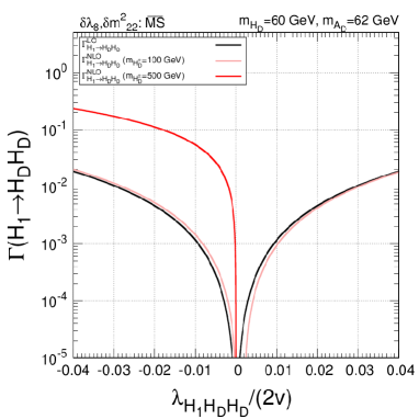
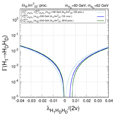
Figure 1: Decay width $H_{1}\to H_{D}H_{D}$ at LO and NLO as a function of the tree-level coupling $\lambda_{H_{1}H_{D}H_{D}}$ for $m_{H_{D}}=60$ GeV and $m_{A_{D}}=62$ GeV, and for two different values of $m_{H_{D}^{\pm}}$, $m_{H_{D}^{\pm}}=100$ and 500 GeV. The variable $m_{22}^{2}$ is scanned in a range such that the DM direct detection constraints hold. Other input parameters are fixed to the values given in Eqs. (83), (84) and (85). The left panel shows the results for the $\overline{\rm MS}$ scheme, while the right panel presents results for the two process-dependent schemes.

The remaining 10 parameters, besides the two tadpoles $T_{\Phi}=T_{S}=0$, are set as follows: $H_{1}$ is the SM-like Higgs boson with $m_{H_{1}}=125.09$ GeV, and the mass of the heavier Higgs boson $H_{2}$ is fixed as

$$m_{H_{2}}=500\,{\rm GeV}\;.$$ (83)

The parameters of the dark sector, $m_{H_{D}}$, $m_{H^{\pm}_{D}}$ and $\lambda_{2}$, are set to

$$m_{H_{D}}=50\ \mbox{GeV or }60\leavevmode\nobreak\ {\rm GeV}\,,\quad m_{H^{\pm}_{D}}=100\ \mbox{GeV or }500\ \mbox{GeV}\,,\quad\lambda_{2}=0.12\,,$$ (84)

while the remaining mass parameters $m_{A_{D}}$ and $m^{2}_{22}$ can be either scanned over or fixed in the following plots. We assume $m_{A_{D}}>m_{H_{D}}$, meaning that the dark scalar $H_{D}$ is the DM candidate. As previously stated we choose for $\lambda_{8}$, $\alpha$ and $v_{S}$,

$$\lambda_{8}=0,\ \ \ \alpha=0,\ \ \ v_{S}\to\infty\,,$$ (85)

in that order, which is equivalent to take $m_{S}^{2},\lambda_{6},\lambda_{7}$ and $\lambda_{8}$ equal to zero in the scalar potential in Eq. (2). This is in turn equivalent to the IDM potential. Hence, Eq. (85) gives the IDM limit in the DDP phase of the N2HDM and we should recover the IDM results. When the $\overline{\rm MS}$ scheme is used to calculate $\delta\lambda_{8}$ and $\delta m_{22}^{2}$, the one-loop amplitude for $H_{1}\to H_{D}H_{D}$ depends on the renormalization scale $\mu$ and we set it as $\mu^{2}=m_{H_{1}}^{2}$.

In Fig. 1, we show the correlation between the tree-level coupling $H_{1}H_{D}H_{D}$ and the decay width for the corresponding process $H_{1}\to H_{D}H_{D}$ at LO and NLO and for two different charged Higgs masses, $m_{H_{D}^{\pm}}=100$ GeV and 500 GeV. In this plot, we set the mass of the CP-odd dark scalar to $m_{A_{D}}=62$ GeV and vary $m^{2}_{22}$ in a range that forces the tree-level coupling to be $|\lambda_{H_{1}H_{D}H_{D}}/(2v)|<0.05$  [46]. The upper bound for $|\lambda_{H_{1}H_{D}H_{D}}/(2v)|$ corresponds to the current bounds for direct detection of DM from XENON1T [47]. From the left panel, in which the $\overline{\rm MS}$ scheme results are shown, one can see a parabolic behaviour for the decay width at both LO and NLO, with the width vanishing at $\lambda_{H_{1}H_{D}H_{D}}/(2v)=0$. The most important feature is that the NLO corrections strongly depend on the value of $m_{H_{D}^{\pm}}$ and can be very large even for relatively small $\lambda_{H_{1}H_{D}H_{D}}$ if the mass of the dark charged scalars is large ($m_{H_{D}^{\pm}}=500$ GeV in the plot). In the right panel of Fig. 1, results for the two process-dependent schemes are shown. The behaviour of the results at NLO for $m_{H^{\pm}_{D}}=100$ GeV is similar for all three renormalization schemes. In particular, we have confirmed that the result for the ZEM process-dependent scheme almost coincides with that for the OS process-dependent scheme. However, the NLO corrections for the decay width at $m_{H^{\pm}_{D}}=500$ GeV are quite moderate in both process-dependent schemes, in contrast with the $\overline{\rm MS}$ scheme.

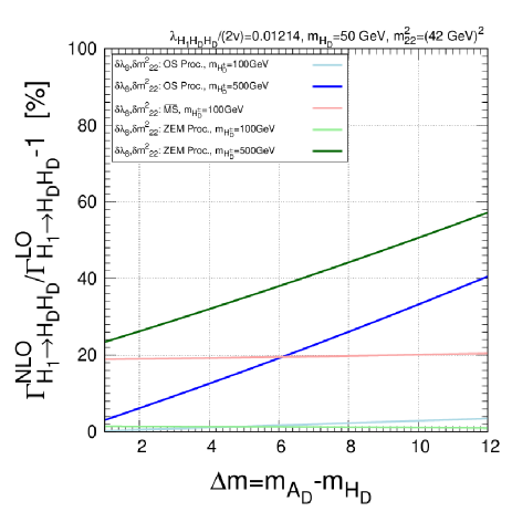
Figure 2: Relative size of the NLO corrections for $H_{1}\to H_{D}H_{D}$ as a function of the mass difference between $H_{D}$ and $A_{D}$, denoted by $\Delta m=m_{A_{D}}-m_{H_{D}}$, and for two different values of $m_{H^{\pm}_{D}}$, $m_{H_{D}^{\pm}}=100$ and 500 GeV. The parameters are chosen as $m_{H_{D}}=50$ GeV and $m_{22}^{2}=(42\ {\rm GeV})^{2}$ while the mass of the CP-odd scalar $m_{A_{D}}$ is scanned keeping $m_{H_{D}}<m_{A_{D}}$. The other input parameters are fixed as in Eqs. (83), (84) and (85). The line colours for the different schemes are explained in the legend.

In Fig. 2, we show the relative size of the NLO corrections

$$\Delta_{\text{NLO}}\equiv\Gamma^{\rm NLO}/\Gamma^{\rm LO}-1$$ (86)

as a function of the mass difference between the CP-odd dark scalar and the CP-even dark scalar, $\Delta m\equiv m_{A_{D}}-m_{H_{D}}$, for the three different renormalization schemes and for two different charged Higgs masses, $m_{H_{D}^{\pm}}=100$ GeV and 500 GeV. The parameters are chosen as $m_{H_{D}}=50\leavevmode\nobreak\ {\rm GeV}$ and $m_{22}^{2}=(42\leavevmode\nobreak\ {\rm GeV})^{2}$, which corresponds to $\lambda_{H_{1}H_{D}H_{D}}/(2v)=0.01214$. The upper limit $\Delta m\lesssim 12$ GeV is used because we want to compare the renormalization schemes in a region where they all can be applied. The SM-like Higgs decay into a pair of CP-odd scalars, $H_{1}\to A_{D}A_{D}$, has to be kinematically allowed so that Eq. (70) is applicable. The NLO corrections for the $\overline{\rm MS}$ scheme, with $m_{H_{D}^{\pm}}$ fixed to 100 GeV, are almost constant, i.e., they do not depend on the mass difference between the two dark neutral scalars. Nonetheless, as we have seen before, they do depend quite strongly on the charged Higgs mass. In both process-dependent schemes, the NLO corrections strongly depend on the mass difference, $\Delta m$, but also on the value of the charged Higgs mass. For a low value of the charged Higgs mass, $m_{H^{\pm}_{D}}=100\,{\rm GeV}$, the maximum value of the relative correction for the process-dependent schemes is $\Delta_{\text{NLO}}$=4% at $\Delta m=12\leavevmode\nobreak\ {\rm GeV}$, while the minimum is $\Delta_{\text{NLO}}\sim 0\%$. These corrections increase for larger charged Higgs mass. Considering $m_{H^{\pm}_{D}}=500\leavevmode\nobreak\ {\rm GeV}$, the value of $\Gamma^{\rm NLO}/\Gamma^{\rm LO}-1$ has a minimum of about 4% (24%) for the OS (ZEM) case for $\Delta m=0$ and a maximum of about 40% (57%) for the OS (ZEM) case for $\Delta m=12\leavevmode\nobreak\ {\rm GeV}$. This behaviour can be understood from the fact that there is a significant number of terms in $\mathcal{M}^{\rm 1\mathchar 45\relax loop}_{H_{1}\to H_{D}H_{D}}$ that are proportional to $\Delta m$ and, consequently, they have a large impact on the one-loop result. The latter is also proportional to the charged Higgs mass and, therefore, sizable corrections are found for $m_{H^{\pm}_{D}}=500$ GeV. In the $\overline{\rm MS}$ scheme, the NLO corrections for $m_{H^{\pm}}=500$ GeV are well above 100% in the entire mass range, $\Delta m\in[0,12]$ GeV, and not shown in the plot.

5.2 Scan Analysis for the Branching Ratios

In this section, we will perform a scan over the allowed parameter space of the model. This will enable us to understand the overall behavior of the NLO corrections to the SM-like Higgs decays into a pair of DM particles. The evaluation of the branching ratio is performed using N2HDECAY [48] which is an extension of the original code HDECAY [49, 50] to the N2HDM. The program computes the branching ratios and the total decay widths of the neutral Higgs bosons $H_{1}$ and $H_{2}$, including the state-of-the art QCD corrections. Using the value of the partial widths evaluated by N2HDECAY, $\Gamma^{\rm N2HDECAY}$, we evaluate the branching ratios for $H_{i}\to H_{D}H_{D}$ with the NLO EW corrections as

$${\rm BR}(H_{i}\to H_{D}H_{D})=\frac{\Gamma^{\rm\tt N2HDECAY}_{H_{i}\to H_{D}H_{D}}(1+\delta^{\rm EW}_{H_{i}\to H_{D}H_{D}})}{\Gamma^{\rm\tt N2HDECAY}_{H_{i}\to\rm SM}+\Gamma_{H_{i}\to\Phi\Phi}}\;,$$ (87)

where the correction factor $\delta^{\rm EW}_{H_{i}\to XX}$ is defined by

$$\delta^{\rm EW}_{H_{i}\to XX}=\frac{\Gamma^{\rm NLO}_{H_{i}\to XX}-\Gamma^{\rm LO}_{H_{i}\to XX}}{\Gamma^{\rm LO}_{H_{i}\to XX}}\,.$$ (88)

In Eq. (87), the total decay width is separated into the decays into the SM particles, $\Gamma^{\rm\tt N2HDECAY}_{H_{i}\to{\rm SM}}$, and the decay into a pair of the scalar bosons $\Gamma_{H_{i}\to\Phi\Phi}$, defined as

$$\Gamma_{H_{1}\to\Phi\Phi} =\Gamma^{\rm\tt N2HDECAY}_{H_{1}\to H_{D}H_{D}}\left(1+\delta^{\rm EW}_{H_{1}\to H_{D}H_{D}}\right)+\Gamma^{\rm\tt N2HDECAY}_{H_{1}\to A_{D}A_{D}}\left(1+\delta^{\rm EW}_{H_{1}\to A_{D}A_{D}}\right)+\Gamma^{\rm\tt N2HDECAY}_{H_{1}\to H^{+}_{D}H^{-}_{D}}\,,$$ (89)

$$\Gamma_{H_{2}\to\Phi\Phi} =\Gamma^{\rm\tt N2HDECAY}_{H_{2}\to H_{D}H_{D}}(1+\delta^{\rm EW}_{H_{2}\to H_{D}H_{D}})+\Gamma^{\rm\tt N2HDECAY}_{H_{2}\to A_{D}A_{D}}\left(1+\delta^{\rm EW}_{H_{2}\to A_{D}A_{D}}\right)$$

$$+\Gamma^{\rm\tt N2HDECAY}_{H_{2}\to H_{D}^{+}H_{D}^{-}}+\Gamma^{\rm\tt N2HDECAY}_{H_{2}\to H_{1}H_{1}}\,,$$ (90)

where we include our computed EW corrections to the decays into neutral dark bosons, $H_{i}\to H_{D}H_{D}$ and $H_{i}\to A_{D}A_{D}$. Here we highlight that, in the process-dependent scheme, $\delta^{\rm EW}_{H_{i}\to A_{D}A_{D}}$ disappears because of the renormalization condition Eq. (70).

We consider two different scenarios in our scan. In scenario 1, the lighter Higgs boson $H_{1}$ is identified as the SM-like Higgs boson and the other CP-even Higgs boson $H_{2}$ is heavier than the SM-like Higgs boson. In scenario 2, $H_{2}$ is the SM-like Higgs boson and the other Higgs boson $H_{1}$ is lighter than the SM-like Higgs boson. In both scenarios, the dark scalar $H_{D}$ is the DM candidate. The scan is performed for the two scenarios to examine the impact of the NLO corrections in the allowed parameter space. We use for both scenarios the following ranges for the parameters,

$$1\leavevmode\nobreak\ {\rm GeV}<m_{H_{D}}<62\leavevmode\nobreak\ {\rm GeV}\,,\ \ \ 1\leavevmode\nobreak\ {\rm GeV}<m_{A_{D}}<1500\leavevmode\nobreak\ {\rm GeV}\,\,\,\,(m_{A_{D}}>m_{H_{D}})$$

$$65\leavevmode\nobreak\ {\rm GeV}<m_{H^{\pm}_{D}}<1500\leavevmode\nobreak\ {\rm GeV}\,,\ \ \ 10^{-3}\leavevmode\nobreak\ {\rm GeV}^{2}<m_{22}^{2}<5\cdot 10^{5}\leavevmode\nobreak\ {\rm GeV}^{2}\,,$$

$$1\leavevmode\nobreak\ {\rm GeV}<v_{S}<5000\leavevmode\nobreak\ {\rm GeV}\,,\ \ \ -\pi/2<\alpha<\pi/2\,,$$

$$0<\lambda_{2}<4\pi\,,\ \ \ -4\pi<\lambda_{8}<4\pi\,.$$ (91)

We chose $m_{H_{D}^{\pm}}$ to be above 65 GeV to prevent the SM-like Higgs boson decay into a pair of charged Higgs particles. Additionally, $\lambda_{2}$ is set positive due to the boundedness from below (BFB) conditions, see [8] for details on BFB of the N2HDM.

In scenario 1, the masses of the CP-even Higgs bosons are set as

$$m_{H_{1}}=125.09\leavevmode\nobreak\ {\rm GeV},\quad 130\leavevmode\nobreak\ {\rm GeV}<m_{H_{2}}<1500\leavevmode\nobreak\ {\rm GeV}.$$ (92)

In scenario 2, they are taken as

$$1\leavevmode\nobreak\ {\rm GeV}<m_{H_{1}}<120\leavevmode\nobreak\ {\rm GeV},\quad m_{H_{2}}=125.09\leavevmode\nobreak\ {\rm GeV}.$$ (93)

Since we focus on the case where ${H_{D}}$ is the DM particle, we assume $m_{H_{D}}<m_{A_{D}}$.

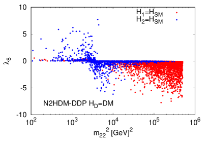
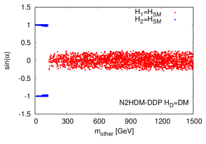
Figure 3: Projections of the allowed parameter space in the planes $(\lambda_{8},\,m_{22}^{2})$ (left) and $(\sin\alpha,m_{\text{other}})$ (right), where $m_{\text{other}}$ is the mass of the non-SM-like Higgs boson. The red points are for scenario 1 and the blue points are for scenario 2.

Using ScannerS [51, 52], we generate input parameter points that pass the most relevant theoretical and experimental constraints. For the theoretical constraints [8, 4], ScannerS evaluates perturbative unitarity, boundedness from below and vacuum stability. The following experimental constraints are taken into account: electroweak precision data, Higgs measurements, Higgs exclusion limits, and DM constraints. These constraints are included in ScannerS via the interface with other high energy physics codes: HiggsBounds-5 [53] for the Higgs searches and HiggsSignals-2 [54] for the constraints of the SM-like Higgs boson measurements. For the DM constraints, the relic abundance and the nucleon-DM cross section for direct detection are calculated by MicroOMEGAs-5.2.4 [55, 56, 57]. The DM relic abundance has to be below the value measured by the Plank experiment [58] and the DM-nucleon cross section has to be within the bounds imposed by the XENON1T [47] results. All points presented in the plots have passed all the above constraints. In Fig. 3 we show two projections of the allowed parameter space in the planes $(\lambda_{8},\,m_{22}^{2})$ (left) and $(\sin\alpha,m_{\text{other}})$ (right), where $m_{\text{other}}$ is the mass of the non-SM-like Higgs boson.

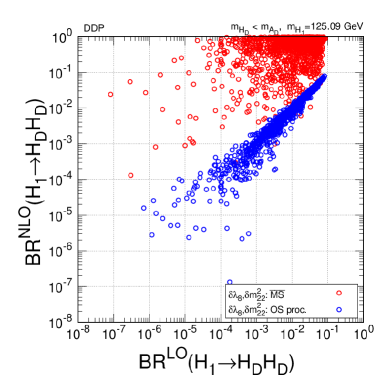
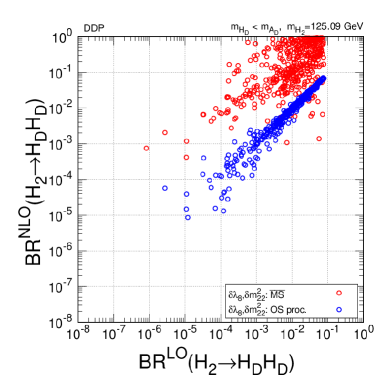
Figure 4: Correlation between the branching ratios at NLO and at LO in scenario 1 (left) and scenario 2 (right), respectively. The red and blue points correspond to results in the $\overline{\rm MS}$ scheme and in the OS process-dependent scheme, respectively.

The red points are for scenario 1 and the blue points are for scenario 2. There are no particularly important features in the parameters $\lambda_{8}$ and $m_{22}^{2}$ that probe the dark sector as expected, except for theoretical constraints that limit the quartic couplings. As for $\sin\alpha$, due to the very SM-like behaviour of the discovered Higgs boson, $\sin\alpha$ is either close to zero or close to $\pm$1, depending on the considered scenario.

In Fig. 4, we show the correlation between the BR$({H_{i}\to H_{D}H_{D}})$ calculated at LO and at NLO in scenario 1 (left panel) and in scenario 2 (right panel). The red and blue points correspond to the calculations in the $\overline{\rm MS}$ scheme and in the OS process-dependent scheme, respectively. This sample has points with $m_{A_{D}}<125/2$ GeV. The first important thing to note is that in both scenarios the LO BR is always below 10%. The main reason for this to happen is the very precise measurements of the Higgs couplings to SM particles which indirectly limit the Higgs coupling to new particles.

The NLO corrections have a very different behaviour in the two renormalization schemes presented. For the $\overline{\rm MS}$ scheme, the NLO corrections are not reliable with NLO BRs reaching 100% in both scenarios. Conversely, the OS process-dependent scheme is better behaved. This behaviour, in the OS scheme, can be traced back to the suppression of the NLO corrections by the mass difference between $H_{D}$ and $A_{D}$, as explained in Sec. 5.1. In our analysis, the mass difference is in the range $0\leavevmode\nobreak\ {\rm GeV}\lesssim\Delta m\lesssim 6\leavevmode\nobreak\ {\rm GeV}$ which leads to small corrections in the OS process-dependent scheme.

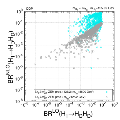
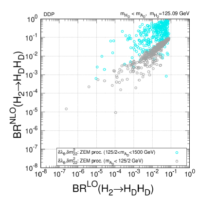
Figure 5: Correlation between the branching ratios at NLO and at LO in scenario 1 (left) and scenario 2 (right). All points have been obtained in the ZEM process-dependent scheme. The grey points correspond to the previous sample where $m_{A_{D}}<125/2$ GeV, while the blue points correspond to a range that is only allowed in the ZEM scheme, $125/2$ GeV$<m_{A_{D}}<1500$ GeV.

In Fig. 5, we show results for the ZEM process-dependent scheme. Again we display the correlation between the branching ratios at NLO and at LO in scenario 1 (left panel) and scenario 2 (right panel). We show results for two different samples of points, all calculated in the ZEM scheme. The grey points correspond to the previous sample where $m_{A_{D}}<125/2$ GeV, while the blue points correspond to a range that is only allowed in the ZEM scheme, $125/2$ GeV$<m_{A_{D}}<1500$ GeV. The points for which $m_{A_{D}}<125/2$ have an overall similar behaviour as the ones for the OS scheme, in the sense that the NLO BRs are all below 0.1. However, one can see that the corrections are much larger, even for this sample. When we look at the blue points the picture changes radically. This clearly shows that when the mass difference between $H_{D}$ and $A_{D}$ is large the corrections become unstable.

In order to understand to what extend these corrections depend on the renormalization schemes, we show, in Fig. 6, the ratio of NLO to LO corrections for the processes ${\rm BR}(H_{1}\to H_{D}H_{D})$ (left panel) and ${\rm BR}(H_{2}\to H_{D}H_{D})$ (right panel). Here again the sample used is the one where $m_{A_{D}}<125/2$ GeV. The red, blue and grey points correspond to the $\overline{\rm MS}$, OS process-dependent and ZEM process-dependent renormalization schemes, respectively. The black horizontal lines corresponds to ${\rm BR}^{\rm NLO}/{\rm BR}^{\rm LO}-1=\pm 50\%$. The plots clearly show that the OS process-dependent scheme is more stable with most corrections between -50% and 50%. In any case, the corrections in this scheme can still go up to 480%. As the corrections above 100% only occur for small values of the LO BRs, the NLO values of the BRs are still well below the experimental bound. The other two schemes are less stable and this is particularly true for the $\overline{\rm MS}$ scheme.

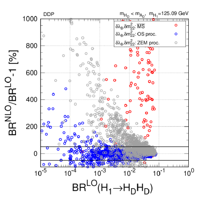
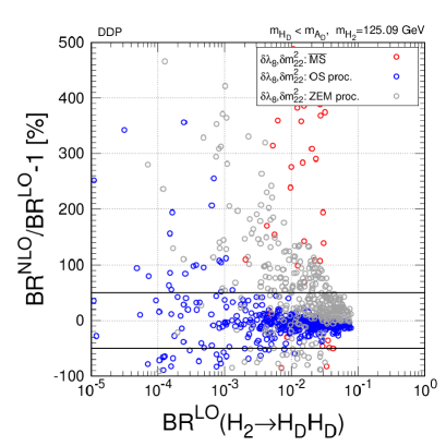
Figure 6: Ratio of NLO to LO corrections for ${\rm BR}(H_{i}\to H_{D}H_{D})$ in scenario 1 (left) and scenario 2 (right). The red, blue and grey points correspond to the $\overline{\rm MS}$, ZEM process-dependent and OS process-dependent scheme, respectively. The black horizontal lines correspond to ${\rm BR}^{\rm NLO}/{\rm BR}^{\rm LO}-1=\pm 50\%$.

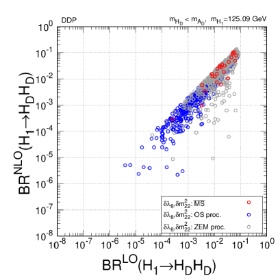
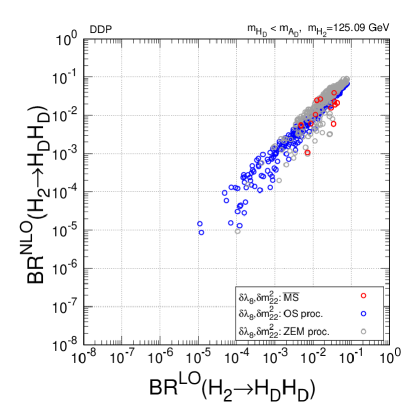
Figure 7: Correlation between the branching ratios at NLO and at LO in scenario 1 (left) and scenario 2 (right), respectively. The red, blue and grey points correspond to the $\overline{\rm MS}$, OS process-dependent and ZEM process-dependent scheme, respectively.

A clearer picture of the results for the NLO corrections that can be trusted in terms of perturbation theory can be achieved by considering only the points for which the corrections are below 100%. In Fig. 7, we present the correlation between the branching ratios at NLO and at LO in scenario 1 (left panel) and scenario 2 (right panel), respectively. All points presented have NLO corrections below 100% and all points with NLO corrections above 100% were discarded. We conclude that the surviving points are all still below the current experimental limit for the Higgs invisible BR apart from a few grey points. One should keep in mind the theoretical uncertainties due to missing higher-order corrections. Additionally, the other decay channels do not include electroweak corrections, which has an impact on the branching ratios. Given these caveats, the points can still be considered compatible with the experimental results. Therefore, no constraints on the parameter space come from including the NLO corrections. However, as the limit on the Higgs invisible BR improves, there are now ranges of allowed values for the NLO corrections that will certainly lead to constraints on the parameter space.

We end this section with a comment about the case where $A_{D}$ is the DM candidate. We have also calculated the NLO corrections to Higgs boson invisible decays in the case that $A_{D}$ is the DM particle. The renormalization was done using the process dependent scheme with the decay $H_{i}\to H_{D}H_{D}$ ($i=1,2$), i.e., $\Gamma_{H_{i}\to H_{D}H_{D}}^{\rm LO}\overset{!}{=}\Gamma_{H_{i}\to H_{D}H_{D}}^{\rm NLO}$ and we have performed the same scan analysis presented above for $H_{D}$. We confirm that the results are virtually identical with those obtained for $H_{D}$, in both scenarios 1 and 2.

6 Conclusions

In this work we have calculated the EW NLO corrections to the branching ratio of the SM-like Higgs boson invisible decay in the DDP of the N2HDM. We have analysed two different scenarios, one where the SM-like Higgs is the lighter of the visible two CP-even scalars and one where it is the heavier. There are, however, no significant differences between the two scenarios. The model has 13 input parameters from the scalar sector. Masses and wave function renormalization constants are renormalized on-shell. The rotation angle is renormalized by relating the fields in the gauge basis and in the mass basis and it is ultimately defined with the off-diagonal terms of the wave function renormalization constants. We apply a gauge-independent renormalization scheme based on the alternative tadpole scheme together with the pinch technique. Besides the EW VEV, that is renormalized exactly like in the SM, we still have four parameters left: $\lambda_{2}$ (which does not enter in any of the processes under study), $\lambda_{8}$, $m_{22}^{2}$ and $v_{S}$.

Regarding $\lambda_{8}$ and $m_{22}^{2}$ the analysis was performed for three different renormalization schemes. The three schemes used for these parameters were the $\overline{\rm MS}$, the OS process-dependent and the ZEM process-dependent scheme. Only in the first one does $v_{S}$ need to be renormalized. The most stable scheme is the OS process-dependent one, but it can still lead to corrections above 100 % in some regions of the parameter space. It should be noted that one of the reasons for the OS scheme stability is that the mass difference between the two neutral dark scalars, $m_{A_{D}}-m_{H_{D}}$, is bounded to be below about 10 GeV. Note that the OS process-dependent scheme needs an allowed on-shell decay of the SM-like Higgs boson to both pairs of dark scalars.

With the LHC run 3 starting soon, the Higgs coupling and the invisible Higgs decay width measurements will become increasingly precise. It is clearly the time to understand what the NLO corrections can tell us about the models with more precise measurements. In fact, these experimental results can be the best, if not the only, tools available to probe the dark sectors postulated as extensions of the SM. One should stress that the parameters $\lambda_{8}$ and $m_{22}^{2}$ are only directly accessible through processes that involve the DM particles. The experimental sensitivity on the invisible decay width is now starting to become comparable to the limits imposed on the parameter space of the model from the coupling measurements.

We have found that the NLO corrections can be extremely large in some regions of the parameter space. Also, as we move to smaller values of the ${\rm BR}(H_{i}\to H_{D}H_{D})$, the corrections become larger and larger. This means that the more constrained the BR is the more unstable are the NLO corrections. As a perturbativity criteria, we rejected all points for which the NLO corrections relative to the LO results are above 100%. With this condition, the behaviour of NLO versus LO results is very much along the line BR${}^{\text{NLO}}=$ BR${}^{\text{LO}}$. Still, if the experimental bound of $BR(h\to$ invisible) improves, for instance to $10^{-2}$, the NLO result would vary between $\sim 10^{-4}$ to $\sim 2\times 10^{-2}$ .

Appendix

Appendix A Determination of $\delta\lambda_{8}$ and $\delta m_{22}^{2}$ in the Process-Dependent Scheme

In this appendix, we discuss how the counterterms $\delta\lambda_{8}$ and $\delta m^{2}_{22}$ are determined using the process-dependent scheme. As previously discussed, although our starting point is to force the amplitudes at LO and at NLO to be equal, we choose two different approaches. In one approach all particles are on-shell, which is equivalent to say that the condition is set on the actual physical process. In the other approach, the condition is set at the amplitude level taking all external momenta to be zero. The advantage of this second approach is not to curtail the allowed parameter space.

We will now describe in detail the renormalization procedure for the on-shell case and discuss the differences when the external momenta are set to zero at the end of this appendix. The on-shell process-dependent renormalization condition is to impose the decay widths for $H_{i}\to A_{D}A_{D}$ (i=1,2) calculated at NLO to be equal to the LO result, as expressed in Eq. (70) and repeated here for convenience,

$$\Gamma_{H_{i}\to A_{D}A_{D}}^{\rm LO}\overset{!}{=}\Gamma_{H_{i}\to A_{D}A_{D}}^{\rm NLO}\quad(i=1,2)\,.$$ (94)

This results in two equations where $\delta\lambda_{8}$ and $\delta m_{22}^{2}$ are the only unknowns. The remaining renormalization constants are all fixed. Solving this set of equations, we can get expressions for these two counterterms. The renormalization conditions, given in Eq. (94), can be written as

$$\frac{1}{2}\frac{1}{2m_{H_{i}}}\int d\Phi_{2}|\mathcal{M}_{i}^{\rm tree}|^{2} =\frac{1}{2}\frac{1}{2m_{H_{i}}}\int d\Phi_{2}\Big{[}|\mathcal{M}_{i}^{\rm tree}|^{2}+2{\rm Re}\big{(}\mathcal{M}_{i}^{{\rm tree}*}\mathcal{M}_{i}^{{\rm 1\mathchar 45\relax loop}}\big{)}\Big{]}$$

$$0 ={\rm Re}\big{(}\mathcal{M}_{i}^{{\rm tree}*}\mathcal{M}_{i}^{{\rm 1\mathchar 45\relax loop}}\big{)}\,,$$ (95)

where $d\Phi_{2}$ denotes the two-particle differential phase space volume and $\mathcal{M}^{\rm tree/1\mathchar 45\relax loop}_{i}\equiv\mathcal{M}^{\rm tree/1\mathchar 45\relax loop}_{H_{i}\to A_{D}A_{D}}$ ($i=1,2$). The tree-level amplitude is given by

$$\mathcal{M}^{\rm tree}_{i}=\lambda_{H_{i}A_{D}A_{D}}\,,$$ (96)

where the scalar trilinear coupling $\lambda_{H_{i}A_{D}A_{D}}$ is

$$\lambda_{H_{i}A_{D}A_{D}}=-\frac{1}{v}\big{[}2(m_{A_{D}}^{2}-m_{22}^{2})R_{i1}+\lambda_{8}v_{S}(vR_{i3}-v_{S}R_{i1})\big{]}\,.$$ (97)

Taking into account that $\mathcal{M}_{i}^{{\rm tree}}$ is a real constant, the renormalization condition simplifies to

$$0 ={\rm Re}\big{(}\mathcal{M}_{i}^{{\rm 1\mathchar 45\relax loop}}\big{)}\,,$$ (98)

with the one-loop amplitude expressed as

$$\mathcal{M}_{i}^{{\rm 1\mathchar 45\relax loop}}=\mathcal{M}_{i}^{\rm 1PI}+\mathcal{M}_{i}^{\rm CT}|_{\delta\lambda_{8},\ \delta m^{2}_{22}=0}+\mathcal{M}_{i}^{\rm CT}|_{\delta\lambda_{8},\ \delta m^{2}_{22}\neq 0}\,,$$ (99)

where $\mathcal{M}_{i}^{\rm 1PI}$ denotes 1PI diagrams for the loop-corrected decay widths $H_{i}\to A_{D}A_{D}$ and the counterterm contributions are separated into $\delta\lambda_{8}$ and $\delta{m}_{22}^{2}$ dependent terms $\mathcal{M}_{i}^{\rm CT}|_{\delta\lambda_{8},\ \delta m^{2}_{22}\neq 0}$ and the remainder $\mathcal{M}_{i}^{\rm CT}|_{\delta\lambda_{8},\ \delta m^{2}_{22}=0}$. We note that the counterterms for $H_{i}\to A_{D}A_{D}$ can be obtained from those for $H_{i}\to H_{D}H_{D}$, see Eq. (79), with the replacements

$$(m_{H_{D}},\lambda_{H_{i}H_{D}H_{D}},\delta m_{H_{D}}^{2},\delta Z_{H_{D}})\to(m_{A_{D}},\lambda_{H_{i}A_{D}A_{D}},\delta m_{A_{D}}^{2},\delta Z_{A_{D}}).$$ (100)

Hence the counterterm amplitudes can be written as

$$\mathcal{M}_{i}^{\rm CT}|_{\delta\lambda_{8},\ \delta m^{2}_{22}\neq 0} =2\frac{R_{i1}}{v}\delta m^{2}_{22}-\frac{v_{S}}{v}(R_{i3}v-R_{i1}v_{S})\delta\lambda_{8}\,,$$ (101)

$$\mathcal{M}_{i}^{\rm CT}|_{\delta\lambda_{8},\ \delta m^{2}_{22}=0} =-2\Big{[}\frac{R_{i1}}{v}\delta m_{A_{D}}^{2}+\frac{1}{v}(m_{A_{D}}^{2}-m_{22}^{2}-\frac{1}{2}v_{S}^{2}\lambda_{8})\delta R_{i1}+\frac{v_{S}}{2}\delta R_{i3}$$

$$+\frac{R_{i1}}{v^{2}}(m_{22}^{2}-m_{A_{D}}^{2}+\frac{1}{2}v_{S}^{2}\lambda_{8})\Delta v+(\frac{R_{i3}}{2}-R_{i1}\frac{v_{S}}{v})\lambda_{8}\Delta v_{S}\Big{]}$$

$$+\lambda_{H_{i}A_{D}A_{D}}\left(\delta Z_{A_{D}}+\frac{1}{2}\delta Z_{H_{i}}+\frac{1}{2}\frac{\lambda_{H_{j}A_{D}A_{D}}}{\lambda_{H_{i}A_{D}A_{D}}}\delta Z_{H_{j}H_{i}}\right),\ \ \ (j\neq i).$$ (102)

Finally we obtain the following set of equations,

$$2\frac{R_{i1}}{v}\delta m^{2}_{22}-\frac{v_{S}}{v}(R_{i3}v-R_{i1}v_{S})\delta\lambda_{8}=-\mathcal{M}_{i}^{\rm 1PI}-\mathcal{M}_{i}^{\rm CT}|_{\delta\lambda_{8},\ \delta m^{2}_{22}=0}\,,$$ (103)

which give us the expressions for $\delta\lambda_{8}$ and $\delta m^{2}_{22}$. Note that the left-handed side of Eq. (103) corresponds to the linear combinations of $\delta\lambda_{8}$ and $\delta m^{2}_{22}$ that also appear in the counterterms for $H_{i}\to H_{D}H_{D}$.

The second process-dependent scheme, where all external momenta are set to zero, also starts from the same set of Eq. (103). The only difference is in the calculation of $\mathcal{M}_{i}^{\rm 1PI}$ in which the external momenta are set to zero instead of on-shell.

Figure 8: Comparison of the two process-dependent renormalization schemes, on-shell vs. zero external momenta. We show the ratio between the NLO values vs. the corresponding ${\rm BR}(H_{1}\to H_{D}H_{D})$ (left) and ${\rm BR}(H_{2}\to H_{D}H_{D})$ (right) at LO.

The two schemes are compared in Fig. 8, where we plot the ratio of the NLO corrections of the two process-dependent schemes, the zero external momenta over the on-shell scheme, in per-cent, as a function of the LO branching ratio. The left plot corresponds to the decay $H_{1}\to H_{D}H_{D}$ while the right one corresponds to $H_{2}\to H_{D}H_{D}$. We conclude that the differences can be quite large. In fact, although we have cut the $y$-axis at 500 $\%$ for clarity, there are points where the corrections can go above $10^{3}\%$, which, however, is not the case for the larger values of the LO branching ratios. The important point is that very large corrections only occur for the lower values of the BRs so that the NLO results for the larger values of the BRs are quite similar.

Appendix B Derivation of $\Delta v_{S}$

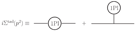
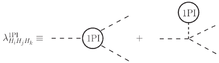
Figure 9: Self-energy diagrams and triangle vertex diagrams in the alternative tadpole scheme.

In this appendix, we derive the analytic expressions for $\Delta v_{S}$ for the case where ${\lambda_{8}}$ and ${m_{22}^{2}}$ are renormalized in the $\overline{\rm MS}$ scheme. As mentioned before, if these parameters are renormalized via a physical process there in no need to renormalize $v_{S}$. We stated in Sec. 3.2.5, that $\delta v_{S}$ is determined such that the remaining UV divergence in the renormalized one-loop amplitude for $H_{1}\to H_{D}H_{D}$ is absorbed by the $\Delta v_{S}$ term in the process.

As schematically depicted in Fig. 9, self-energies and one-loop amplitudes for $H_{1}\to H_{D}H_{D}$ can be separated into two parts: diagrams coming from the traditional tadpole scheme and new diagrams including tadpole contributions due to the alternative tadpole scheme. This is in fact the main difference between the two schemes. Quantities in the usual tadpole scheme will be denoted by $X|_{\rm usual}$ while tadpole contributions for the quantities $X$, which correspond to the second diagrams in Fig. 9, are written as $X|_{\rm tad}$. One can check that, in the usual tadpole scheme, the UV divergences in $\mathcal{M}^{\rm 1-loop}_{H_{1}\to H_{D}H_{D}}$ are cancelled without the need for introducing $\Delta v_{S}$. By using the ${\overline{\rm MS}}$ counterterms $\delta\lambda_{8}$ and $\delta m_{22}^{2}$, we can show that

$$\left.\mathcal{M}^{\rm 1PI}_{H_{1}\to H_{D}H_{D}}\right|_{\rm div,usual}+\left.\mathcal{M}^{\rm CT}_{H_{1}\to H_{D}H_{D}}\right|_{\rm div,usual}^{\Delta v_{S}=0}=0.$$ (104)

In the following paragraphs, we will show that this is not the case in the alternative tadpole scheme. There are UV divergences coming from the tadpole diagrams in the one-loop amplitude $\mathcal{M}^{\rm 1-loop}_{H_{1}\to H_{D}H_{D}}$ that lead to an extra infinity in the amplitude that will be cancelled by the $v_{S}$ counterterm. First, we define the tadpole diagrams as

$$T_{H_{i}}\equiv\includegraphics[width=34.1433pt]{taddiag2.pdf}\vspace{-2.0cm}$$ (105)

where $i=1,2$. Then the tadpole parts of the 1PI diagram contributions are expressed as

$$\left.\mathcal{M}^{\rm 1PI}_{H_{1}\to H_{D}H_{D}}\right|_{\rm tad}=\lambda_{H_{1}H_{1}H_{D}H_{D}}\frac{T_{H_{1}}}{m_{H_{1}}^{2}}+\lambda_{H_{1}H_{2}H_{D}H_{D}}\frac{T_{H_{2}}}{m_{H_{2}}^{2}},$$ (106)

where

$$\lambda_{H_{1}H_{1}H_{D}H_{D}} =\frac{c^{2}_{\alpha}}{v^{2}}(2m_{22}^{2}-2m_{H_{D}}^{2}+\lambda_{8}v_{S}^{2})-s_{\alpha}^{2}\lambda_{8},$$ (107)

$$\lambda_{H_{1}H_{2}H_{D}H_{D}} =-\frac{c_{\alpha}s_{\alpha}}{v^{2}}\Big{\{}2m_{22}^{2}-2m_{H_{D}}^{2}+\lambda_{8}(v_{S}^{2}+v^{2})\Big{\}}.$$ (108)

In the ${\overline{\rm MS}}$ scheme, the counterterms for $\delta\lambda_{8}$ and $\delta m_{22}^{2}$ do not contain tadpole contributions. The same is true for $\delta Z_{H_{D}H_{D}}$ and $\delta Z_{H_{1}H_{1}}$ because they are defined as the derivatives of self-energies. Therefore, they do not contribute to $\mathcal{M}^{\rm CT}_{H_{1}\to H_{D}H_{D}}$, which allows us to write

$$\left.\mathcal{M}_{H_{1}\to H_{D}H_{D}}\right|^{\Delta v_{S}=0}_{\rm tad} =\lambda_{H_{2}H_{D}H_{D}}\left(\frac{1}{2}\delta Z_{H_{2}H_{1}}+\delta\alpha\right)\Bigg{|}_{\rm tad}$$

$$-2\frac{c_{\alpha}}{v^{2}}\left(m_{22}^{2}-m_{H_{D}}^{2}+\frac{1}{2}v_{S}\lambda_{8}\right)\Delta v\big{|}_{\rm tad}-2\frac{c_{\alpha}}{v}\delta m_{H_{D}}^{2}\big{|}_{\rm tad}.$$ (109)

The various terms are given by the following expressions:

• $\underline{\frac{1}{2}\delta Z_{H_{2}H_{1}}+\delta\alpha}$:

  We can see that the tadpole parts are cancelled out:

  $$\left(\frac{1}{2}\delta Z_{H_{2}H_{1}}+\delta\alpha\right)_{\rm tad} =\frac{1}{2}\frac{1}{m_{H_{1}}^{2}-m_{H_{2}}^{2}}\left[\Sigma^{\rm tad}_{H_{1}H_{2}}(m_{H_{2}}^{2})-\Sigma^{\rm tad}_{H_{2}H_{1}}(m_{H_{1}}^{2})\right]\big{|}_{\rm tad}$$

  $$=0,$$ (110)

  where we have used the following expressions for the tadpole parts of $\Sigma_{H_{1}H_{2}}$ and $\Sigma_{H_{2}H_{1}}$

  $$\Sigma^{\rm tad}_{H_{1}H_{2}}|_{\rm tad}=\Sigma^{\rm tad}_{H_{2}H_{1}}|_{\rm tad}=\lambda_{H_{1}H_{D}H_{D}}\frac{T_{H_{1}}}{m_{H_{1}}^{2}}+\lambda_{H_{2}H_{D}H_{D}}\frac{T_{H_{2}}}{m_{H_{2}}^{2}}.$$ (111)

• $\underline{\Delta v}$:

  The tadpole contributions of the gauge boson $(V=Z,W)$ self-energies are given by

  $$\Sigma^{\rm tad}_{VV}|_{\rm tad}=-\left(c_{\alpha}\frac{T_{H_{1}}}{m_{H_{1}}^{2}}-s_{\alpha}\frac{T_{H_{2}}}{m_{H_{2}}^{2}}\right)\,.$$ (112)

  This yields

  $$\frac{\Delta v}{v}\Big{|}_{\rm tad} =\frac{1}{2}\left(\frac{s_{W}^{2}-c_{W}^{2}}{s_{W}^{2}}\frac{1}{m^{2}_{W}}\Sigma_{WW}^{\rm tad}\big{|}_{\rm tad}+\frac{c_{W}^{2}}{s_{W}^{2}}\frac{1}{m^{2}_{Z}}\Sigma_{ZZ}^{\rm tad}\big{|}_{\rm tad}\right)$$ (113)

  $$=-\frac{1}{v}\left(c_{\alpha}\frac{T_{H_{1}}}{m_{H_{1}}^{2}}-s_{\alpha}\frac{T_{H_{2}}}{m_{H_{2}}^{2}}\right).$$

• $\underline{\delta m_{H_{D}}^{2}}$:

  The tadpole contribution for the mass counterterm $\delta m_{H_{D}}^{2}$ reads

  $$\delta m_{H_{D}}^{2}|_{\rm tad}=\lambda_{H_{1}H_{D}H_{D}}\frac{T_{H_{1}}}{m_{H_{1}}^{2}}+\lambda_{H_{2}H_{D}H_{D}}\frac{T_{H_{2}}}{m_{H_{2}}^{2}}\,.$$ (114)

Putting together all the results, the tadpole part of $\mathcal{M}^{\rm 1-loop}_{H_{1}\to H_{D}H_{D}}$can be written as

$$\mathcal{M}^{\rm 1-loop}_{H_{1}\to H_{D}H_{D}}\big{|}_{\rm tad}^{\Delta v_{S}=0} =\lambda_{H_{1}H_{1}H_{D}H_{D}}\frac{T_{H_{1}}}{m_{H_{1}}^{2}}+\lambda_{H_{1}H_{2}H_{D}H_{D}}\frac{T_{H_{2}}}{m_{H_{2}}^{2}}$$

$$+2\frac{c_{\alpha}}{v^{2}}\left(m_{22}^{2}-m_{H_{D}}^{2}+\frac{1}{2}v_{S}\lambda_{8}\right)\left(c_{\alpha}\frac{T_{H_{1}}}{m_{H_{1}}^{2}}-s_{\alpha}\frac{T_{H_{2}}}{m_{H_{2}}^{2}}\right)$$

$$-2\frac{c_{\alpha}}{v}\left(\lambda_{H_{1}H_{D}H_{D}}\frac{T_{H_{1}}}{m_{H_{1}}^{2}}+\lambda_{H_{2}H_{D}H_{D}}\frac{T_{H_{2}}}{m_{H_{2}}^{2}}\right)$$

$$=\frac{T_{H_{1}}}{m_{H_{1}}^{2}}\Big{[}\lambda_{H_{1}H_{1}H_{D}H_{D}}+2\frac{c_{\alpha}}{v^{2}}\left(m_{22}^{2}-m_{H_{D}}^{2}+\frac{1}{2}v_{S}\lambda_{8}\right)-2\frac{c_{\alpha}}{v}\lambda_{H_{1}H_{D}H_{D}}\Big{]}$$

$$+\frac{T_{H_{2}}}{m_{H_{2}}^{2}}\Big{[}\lambda_{H_{1}H_{2}H_{D}H_{D}}-2\frac{c_{\alpha}s_{\alpha}}{v^{2}}\left(m_{22}^{2}-m_{H_{D}}^{2}+\frac{1}{2}v_{S}\lambda_{8}\right)-2\frac{c_{\alpha}}{v}\lambda_{H_{2}H_{D}H_{D}}\Big{]}$$

$$={\lambda_{8}}\left(2\frac{{v_{S}}}{v}c_{\alpha}-s_{\alpha}\right)\delta v_{S}\,.$$ (115)

In the last equality, we have used Eqs. (26), (58),(107) and (108). Because of $(\delta v_{S})_{\rm div}\neq 0$, the UV divergence, which is proportional to $\lambda_{8}$, remains. Apart from this remaining term, we note that terms with $m_{22}^{2}$ as well as $m_{H_{D}}^{2}$ are cancelled out.

The remaining UV-divergent term in Eq. (B) can be absorbed by using the $\Delta{v_{S}}$ dependent part $\mathcal{M}^{\rm 1-loop}_{H_{1}\to H_{D}H_{D}}\big{|}^{\Delta v_{S}\neq 0}$. Hence we set $\Delta v_{s}$ so as to eliminate the divergent part of Eq. (B),

$$\Delta v_{S}=-(\delta v_{S})_{\rm div}.$$ (116)

Consequently, the one-loop amplitude for $H_{1}\to H_{D}H_{D}$ is UV finite.

Acknowledgments

We thank Jorge Romão for fruitful discussions. DA, PG and RS are supported by FCT under contracts UIDB/00618/2020, UIDP/00618/2020, PTDC/FIS-PAR/31000/2017, CERN/FISPAR /0002/2017, CERN/FIS-PAR/0014/2019, and by the HARMONIA project, contract UMO-2015/18/M/ST2/0518. The work of MM is supported by the BMBF-Project 05H18VKCC1, project number 05H2018.

References

- [1] ATLAS collaboration, G. Aad et al., Observation of a new particle in the search for the Standard Model Higgs boson with the ATLAS detector at the LHC, Phys. Lett. B 716 (2012) 1–29, [1207.7214].
- [2] CMS collaboration, S. Chatrchyan et al., Observation of a New Boson at a Mass of 125 GeV with the CMS Experiment at the LHC, Phys. Lett. B 716 (2012) 30–61, [1207.7235].
- [3] ATLAS collaboration, Combination of searches for invisible Higgs boson decays with the ATLAS experiment, .
- [4] I. Engeln, P. Ferreira, M. M. Mühlleitner, R. Santos and J. Wittbrodt, The Dark Phases of the N2HDM, JHEP 08 (2020) 085, [2004.05382].
- [5] C.-Y. Chen, M. Freid and M. Sher, Next-to-minimal two Higgs doublet model, Phys. Rev. D 89 (2014) 075009, [1312.3949].
- [6] A. Drozd, B. Grzadkowski, J. F. Gunion and Y. Jiang, Extending two-Higgs-doublet models by a singlet scalar field - the Case for Dark Matter, JHEP 11 (2014) 105, [1408.2106].
- [7] Y. Jiang, L. Li and R. Zheng, Boosted scalar confronting 750 GeV di-photon excess, 1605.01898.
- [8] M. Muhlleitner, M. O. P. Sampaio, R. Santos and J. Wittbrodt, The N2HDM under Theoretical and Experimental Scrutiny, JHEP 03 (2017) 094, [1612.01309].
- [9] N. G. Deshpande and E. Ma, Pattern of Symmetry Breaking with Two Higgs Doublets, Phys. Rev. D 18 (1978) 2574.
- [10] M. Krause, R. Lorenz, M. Muhlleitner, R. Santos and H. Ziesche, Gauge-independent Renormalization of the 2-Higgs-Doublet Model, JHEP 09 (2016) 143, [1605.04853].
- [11] M. Krause, D. Lopez-Val, M. Muhlleitner and R. Santos, Gauge-independent Renormalization of the N2HDM, JHEP 12 (2017) 077, [1708.01578].
- [12] A. Denner, Techniques for calculation of electroweak radiative corrections at the one loop level and results for W physics at LEP-200, Fortsch. Phys. 41 (1993) 307–420, [0709.1075].
- [13] A. Bredenstein, A. Denner, S. Dittmaier and M. M. Weber, Precise predictions for the Higgs-boson decay H — WW/ZZ — 4 leptons, Phys. Rev. D 74 (2006) 013004, [hep-ph/0604011].
- [14] A. Sirlin, Radiative Corrections in the SU(2)-L x U(1) Theory: A Simple Renormalization Framework, Phys. Rev. D 22 (1980) 971–981.
- [15] J. Fleischer and F. Jegerlehner, Radiative Corrections to Higgs Decays in the Extended Weinberg-Salam Model, Phys. Rev. D 23 (1981) 2001–2026.
- [16] Y. Yamada, Gauge dependence of the on-shell renormalized mixing matrices, Phys. Rev. D 64 (2001) 036008, [hep-ph/0103046].
- [17] J. R. Espinosa and Y. Yamada, Scale independent and gauge independent mixing angles for scalar particles, Phys. Rev. D 67 (2003) 036003, [hep-ph/0207351].
- [18] M. Sperling, D. Stöckinger and A. Voigt, Renormalization of vacuum expectation values in spontaneously broken gauge theories, JHEP 07 (2013) 132, [1305.1548].
- [19] F. Bojarski, G. Chalons, D. Lopez-Val and T. Robens, Heavy to light Higgs boson decays at NLO in the Singlet Extension of the Standard Model, JHEP 02 (2016) 147, [1511.08120].
- [20] M. Krause, M. Muhlleitner, R. Santos and H. Ziesche, Higgs-to-Higgs boson decays in a 2HDM at next-to-leading order, Phys. Rev. D 95 (2017) 075019, [1609.04185].
- [21] A. Denner, L. Jenniches, J.-N. Lang and C. Sturm, Gauge-independent renormalization in the 2HDM, JHEP 09 (2016) 115, [1607.07352].
- [22] L. Altenkamp, S. Dittmaier and H. Rzehak, Renormalization schemes for the Two-Higgs-Doublet Model and applications to h WW/ZZ 4 fermions, JHEP 09 (2017) 134, [1704.02645].
- [23] S. Kanemura, M. Kikuchi, K. Sakurai and K. Yagyu, Gauge invariant one-loop corrections to Higgs boson couplings in non-minimal Higgs models, Phys. Rev. D 96 (2017) 035014, [1705.05399].
- [24] M. Fox, W. Grimus and M. Löschner, Renormalization and radiative corrections to masses in a general Yukawa model, Int. J. Mod. Phys. A 33 (2018) 1850019, [1705.09589].
- [25] A. Denner, S. Dittmaier and J.-N. Lang, Renormalization of mixing angles, JHEP 11 (2018) 104, [1808.03466].
- [26] V. Dūdėnas and M. Löschner, Vacuum expectation value renormalization in the Standard Model and beyond, 2010.15076.
- [27] J. M. Cornwall and J. Papavassiliou, Gauge Invariant Three Gluon Vertex in QCD, Phys. Rev. D 40 (1989) 3474.
- [28] J. Papavassiliou, Gauge independent transverse and longitudinal self energies and vertices via the pinch technique, Phys. Rev. D 50 (1994) 5958–5970, [hep-ph/9406258].
- [29] A. Pilaftsis, Resonant CP violation induced by particle mixing in transition amplitudes, Nucl. Phys. B 504 (1997) 61–107, [hep-ph/9702393].
- [30] S. Kanemura, Y. Okada, E. Senaha and C. P. Yuan, Higgs coupling constants as a probe of new physics, Phys. Rev. D 70 (2004) 115002, [hep-ph/0408364].
- [31] F. Staub, From Superpotential to Model Files for FeynArts and CalcHep/CompHep, Comput. Phys. Commun. 181 (2010) 1077–1086, [0909.2863].
- [32] F. Staub, Automatic Calculation of supersymmetric Renormalization Group Equations and Self Energies, Comput. Phys. Commun. 182 (2011) 808–833, [1002.0840].
- [33] F. Staub, SARAH 3.2: Dirac Gauginos, UFO output, and more, Comput. Phys. Commun. 184 (2013) 1792–1809, [1207.0906].
- [34] F. Staub, SARAH 4 : A tool for (not only SUSY) model builders, Comput. Phys. Commun. 185 (2014) 1773–1790, [1309.7223].
- [35] F. Staub, Exploring new models in all detail with SARAH, Adv. High Energy Phys. 2015 (2015) 840780, [1503.04200].
- [36] G. ’t Hooft and M. J. G. Veltman, Scalar One Loop Integrals, Nucl. Phys. B 153 (1979) 365–401.
- [37] N. D. Christensen and C. Duhr, FeynRules - Feynman rules made easy, Comput. Phys. Commun. 180 (2009) 1614–1641, [0806.4194].
- [38] C. Degrande, C. Duhr, B. Fuks, D. Grellscheid, O. Mattelaer and T. Reiter, UFO - The Universal FeynRules Output, Comput. Phys. Commun. 183 (2012) 1201–1214, [1108.2040].
- [39] A. Alloul, N. D. Christensen, C. Degrande, C. Duhr and B. Fuks, FeynRules 2.0 - A complete toolbox for tree-level phenomenology, Comput. Phys. Commun. 185 (2014) 2250–2300, [1310.1921].
- [40] J. Kublbeck, M. Bohm and A. Denner, Feyn Arts: Computer Algebraic Generation of Feynman Graphs and Amplitudes, Comput. Phys. Commun. 60 (1990) 165–180.
- [41] T. Hahn, Generating Feynman diagrams and amplitudes with FeynArts 3, Comput. Phys. Commun. 140 (2001) 418–431, [hep-ph/0012260].
- [42] R. Mertig, M. Bohm and A. Denner, FEYN CALC: Computer algebraic calculation of Feynman amplitudes, Comput. Phys. Commun. 64 (1991) 345–359.
- [43] V. Shtabovenko, R. Mertig and F. Orellana, New Developments in FeynCalc 9.0, Comput. Phys. Commun. 207 (2016) 432–444, [1601.01167].
- [44] T. Hahn and M. Perez-Victoria, Automatized one loop calculations in four-dimensions and D-dimensions, Comput. Phys. Commun. 118 (1999) 153–165, [hep-ph/9807565].
- [45] G. J. van Oldenborgh and J. A. M. Vermaseren, New Algorithms for One Loop Integrals, Z. Phys. C 46 (1990) 425–438.
- [46] G. Arcadi, A. Djouadi and M. Raidal, Dark Matter through the Higgs portal, Phys. Rept. 842 (2020) 1–180, [1903.03616].
- [47] XENON collaboration, E. Aprile et al., Dark Matter Search Results from a One Ton-Year Exposure of XENON1T, Phys. Rev. Lett. 121 (2018) 111302, [1805.12562].
- [48] I. Engeln, M. Mühlleitner and J. Wittbrodt, N2HDECAY: Higgs Boson Decays in the Different Phases of the N2HDM, Comput. Phys. Commun. 234 (2019) 256–262, [1805.00966].
- [49] A. Djouadi, J. Kalinowski and M. Spira, HDECAY: A Program for Higgs boson decays in the standard model and its supersymmetric extension, Comput. Phys. Commun. 108 (1998) 56–74, [hep-ph/9704448].
- [50] A. Djouadi, J. Kalinowski, M. Muehlleitner and M. Spira, HDECAY: Twenty++ years after, Comput. Phys. Commun. 238 (2019) 214–231, [1801.09506].
- [51] R. Coimbra, M. O. P. Sampaio and R. Santos, ScannerS: Constraining the phase diagram of a complex scalar singlet at the LHC, Eur. Phys. J. C 73 (2013) 2428, [1301.2599].
- [52] M. Mühlleitner, M. O. P. Sampaio, R. Santos and J. Wittbrodt, ScannerS: Parameter Scans in Extended Scalar Sectors, 2007.02985.
- [53] P. Bechtle, D. Dercks, S. Heinemeyer, T. Klingl, T. Stefaniak, G. Weiglein et al., HiggsBounds-5: Testing Higgs Sectors in the LHC 13 TeV Era, 2006.06007.
- [54] P. Bechtle, S. Heinemeyer, T. Klingl, T. Stefaniak, G. Weiglein and J. Wittbrodt, HiggsSignals-2: Probing new physics with precision Higgs measurements in the LHC 13 TeV era, Eur. Phys. J. C 81 (2021) 145, [2012.09197].
- [55] G. Belanger, F. Boudjema, A. Pukhov and A. Semenov, MicrOMEGAs 2.0: A Program to calculate the relic density of dark matter in a generic model, Comput. Phys. Commun. 176 (2007) 367–382, [hep-ph/0607059].
- [56] G. Belanger, F. Boudjema, A. Pukhov and A. Semenov, Dark matter direct detection rate in a generic model with micrOMEGAs 2.2, Comput. Phys. Commun. 180 (2009) 747–767, [0803.2360].
- [57] G. Bélanger, F. Boudjema, A. Goudelis, A. Pukhov and B. Zaldivar, micrOMEGAs5.0 : Freeze-in, Comput. Phys. Commun. 231 (2018) 173–186, [1801.03509].
- [58] Planck collaboration, N. Aghanim et al., Planck 2018 results. VI. Cosmological parameters, Astron. Astrophys. 641 (2020) A6, [1807.06209].