Goodness of fit for log-linear ERGMs

Abstract

Many popular models from the networks literature can be viewed through a common lens of contingency tables on network dyads, resulting in log-linear ERGMs: exponential family models for random graphs whose sufficient statistics are linear on the dyads. We propose a new model in this family, the $p_{1}$-SBM, which combines node and group effects common in network formation mechanisms. In particular, it is a generalization of several well-known ERGMs including the stochastic blockmodel for undirected graphs, the degree-corrected version of it, and the directed $p_{1}$ model without group structure.

We frame the problem of testing model fit for the log-linear ERGM class through an exact conditional test whose $p$-value can be approximated efficiently in networks of both small and moderately large sizes. The sampling methods we build rely on a dynamic adaptation of Markov bases. We use quick estimation algorithms adapted from the contingency table literature and effective sampling methods rooted in graph theory and algebraic statistics. The performance and scalability of the method is demonstrated on two data sets from biology: the connectome of C. elegans and the interactome of Arabidopsis thaliana. These two networks—a neuronal network and a protein-protein interaction network—have been popular examples in the network science literature. Our work provides a model-based approach to studying them.

Keywords: exponential random graph models, networks, log-linear models, Goodness-of-fit, sparse contingency tables, Markov basis

1 Introduction

Data in the form of graphs are common in many biological contexts. In systems biology, graphs are used to record protein-protein interactions. For example, in Arabidopsis Interactome Mapping Consortium (2011), the authors construct a network from 5664 experimentally observed interactions between 2661 proteins from Arabidopsis thaliana, a small flowering plant used as a model organism. In neuroscience, graphs are used to record synaptic contacts between neurons, as in the gap junction and chemical synapse networks constructed for C. elegans in Watts and Strogatz (1998); see also a recent study of these networks in Varshney et al. (2011). Both protein-protein interaction networks and neuronal networks have been used as examples of scale-free networks, that is, networks whose degree distribution follows a power law (Jeong et al. (2000), Tanaka (2005), Wagner and Fell (2001), Albert (2005), Clauset et al. (2009), Bentley et al. (2016)). Descriptive statistics have been used to study these networks, suggesting a degree-based edge formation mechanisms in these data. However, both of these networks have yet to be rigorously analyzed using a model-fitting approach. Part of the difficulty in studying such networks within a model-based setting is that statistical theory regarding fitting random graph models is still in development, since it poses several challenging combinatorial and algorithmic problems.

The present manuscript adds a chapter to the 40-year-long story on random graph models and the difficult question of testing model fit. Even for exponential family random graph models (ERGMs), general quantitative methods for goodness-of-fit testing are still lacking; see for example Kolaczyk (2017, §2.3.4). However, a peek back at the literature over the last four decades suggests that implementable goodness-of-fit methods based on conditional exact tests are, in fact, within reach, especially if we begin by restricting to ERGMs that can be interpreted as log-linear models on contingency tables. Such models are well-known as dyad-independent models in the network modeling literature; see Remark 2.2. While this class of models is a restricted class that does not allow for modeling transitivity, they have found many applications from political blog networks Lei (2016) to financial networks Barucca and Lillo (2016) to biological networks Cabreros et al. (2016), Pavlovic et al. (2014). The class includes, as we discuss in Section 2.1, undirected and directed degree-based models, the stochastic blockmodel (SBM), the degree-corrected version of the SBM, and all of the above which include node covariate information. The stochastic block model and its variants are perhaps the most broadly used due to their connection to clustering (for reviews see Funke and Becker (2019) and Lee and Wilkinson (2019)). Indeed due to their applications to clustering, as argued in Lee and Wilkinson (2019), goodness-of-fit tests for these models are needed for selection and diagnostics during the clustering process.

The following brief historical overview will further illuminate the motivation for our work. The connection between random graph models and log-linear models was made concretely in Fienberg and Wasserman (1981b), a comment on Holland and Leinhardt (1981) that introduced the $p_{1}$ model, a degree-based model for directed networks. The comment paper re-interpreted the model in log-linear form by organizing the network data into a four-dimensional table, thus drawing a natural connection to contingency tables, with each cell representing a classification of a dyad according to the particular state in the observed network. Fienberg and Wasserman (1981b) proved the equivalence of the network and table models, linking random graphs to the exciting developments in categorical data analysis that were taking place at that time and, consequently, to the fitting methods developed over the years and discussed below. The advantage of log-linear model representation to parameter estimation via iterative proportional scaling algorithms was made clear, even if it required a slight redundancy in the data representation. The connection inspired further work: during the same decade, Fienberg et al. (1985) introduced the first variants of the stochastic blockmodel for directed networks, also log-linear in form, which Holland et al. (1983) extended by allowing latent block assignment. More recently, Yan et al. (2019) discuss the asymptotic theory of the directed network model with covariates, a model whose log-linear interpretation is given in Fienberg and Rinaldo (2012).

The decades that followed Fienberg and Wasserman (1981b) saw a flurry of network modeling activity, starting with the early works of Wasserman and Pattison (1996), Pattison and Wasserman (1999), and Robins et al. (1999) who introduced the more general class of ERGMs that included dyad dependent models, building on Markov graphs of Frank and Strauss (1986). Since then, the network modeling literature has begun to address the implementation of goodness-of-fit and hypothesis testing algorithms for specific models, specific families of models, or specific tasks. An early example includes the Conditional Uniform Graphs test Anderson et al. (1999), which compares a graph statistic against an empirical distribution of the statistic obtained by randomly sampling uniformly from the space of all graphs with the same number of vertices and edges. More recently, Lei (2016) provides an asymptotic test for the basic variant stochastic blockmodel, along with a non-asymptotic version, while Banerjee and Ma (2017) offer a hypothesis test for the stochastic blockmodel vs. the Erdös-Rényi model, with optimality guarantees under certain degree growth conditions. For general ERGMs, the question of testing model goodness of fit has been generally acknowledged as difficult. It took until 2008 for the first comprehensive, albeit heuristic, approach to appear in Hunter et al. (2008b) along with an R package for network models; see also Carnegie et al. (2015). The approach in Hunter et al. (2008b) is for general ERGMs, however, the method is graphical, relying on the user to visually assess plots of local summary statistics.

Notable in the literature is the apparent divergence of focus between contingency table models and network models in practice. On the one hand, the network literature generally embraces powerful and fast algorithms rooted in graph theory. Two illustrative examples, Blitzstein and Diaconis (2010) and Zhang and Chen (2013), use sequential importance sampling (SIS) to sample graphs with a prescribed network statistic - the degree sequence in this case. The approach, applicable to a small number of log-linear models, is computationally effective, and represents one of the two main approaches to goodness-of-fit testing based on running a finite-sample algorithm; see also the package Admiraal and Handcock (2008). On the other end of the spectrum, the contingency table literature offers a series of exciting breakthroughs that apply directly to the question of goodness of fit. For all log-linear models for categorical data, the goodness-of-fit question has been theoretically answered nearly three decades ago: Diaconis and Sturmfels (1998) propose a Monte Carlo Markov chain algorithm to compute a finite-sample approximation of an exact conditional test. The framework is guaranteed to work in all log-linear settings, though since it requires the computation of a Markov basis, methods for an effective implementation have remained elusive.

Our mission is to connect the two—graph-based and table-based approaches—and apply the combined theory to fitting a wide class of ERGMs. We take inspiration from Fienberg et al. (2010) and Ogawa et al. (2013) (cf. Petrović et al. (2010), which appeared in the same volume as the latter), who have adapted the Markov bases approach to network applications specifically, and who first demonstrated the feasibility of the method in practice despite apparent theoretical barriers to Markov bases, all of which we discuss below.

Section 2 defines the class of log-linear models for networks in Definition 2.1 and provides the correspondence to contingency tables explicitly. Definition 2.3 constructs a new log-linear ERGM, $p_{1}$-SBM, encapsulating all ‘mix-and-match’ model variants for ‘micro- and macro-analyses of sociometric relations’ as suggested by Fienberg et al. (1985). In Section 3, we formulate a combinatorially modified Metropolis-Hastings algorithm for general log-linear ERGMs. The algorithm has two main parts: Algorithms 1 and 2; the latter is a combinatorial formulation of an efficient Markov basis sampler for each model to which it is applied. We provide the full theory and implementation for models discussed in Section 2, with proof of correctness for those models in Proposition 3.3. Theorem 3.1 specifies exactly what needs to be implemented for any other log-linear ERGM in order for Algorithm 1 to produce, with probability $1$, the exact conditional $p$-value of model fit. We demonstrate the test on simulated and real data sets of medium to moderately large size. One of the data sets includes a large number of structural zeros in the model, rendering standard algebraic statistics methods for testing model fit inapplicable. The proof of Theorem 3.1 discusses why our algorithm is still correct in this scenario, and how it extends the standard Markov basis chain. We close with a discussion of the larger methodological context of our contributions and an outline of some open problems that remain.

Let us briefly address some common concerns with the algebraic statistics approach, details of the solutions to which are in the technical sections that follow. While the method relying on Markov bases is theoretically sound, it can exhibit difficulties in implementation and practice, depending on the approach. For example, Zhang and Chen (2013) pointed to the computational complexity of obtaining a full Markov basis and the limited results on mixing times. However, since the publication of Zhang and Chen (2013), there has been work to address both of these issues. Indeed, dynamic approaches to generating Markov bases elements, such as Dobra (2012) and Ogawa et al. (2013), remedy the computational strain of computing full bases. More recently, Gross et al. (2016) implement the exact conditional test for one variant of the $p_{1}$ random directed graph model of Holland and Leinhardt (1981) with dyad-dependent reciprocation in a combinatorial fashion, avoiding the usual computational bottleneck by constructing one Markov move at a time based on the current state of the chain, rather than precomputing the full basis. We take into account all of these developments within Algorithms 1 and 2.

2 Log-linear ERGMs

Ever since Moreno (1934)’s sociograms, it is well known that network data are best represented as graphs of nodes—or vertices—and edges. We denote the (fixed) number of nodes in the network by $n$, and the class of all graphs on $n$ nodes by $\mathcal{G}_{n}$. Depending on the application, one may restrict the set $\mathcal{G}_{n}$ to simple or multiple (valued), undirected or directed graphs, or a mixture of these, as desired for each model. An exponential family random graph model (ERGM) is a collection of probability distributions on the (possibly restricted) sample space $\mathcal{G}_{n}$ for which the probability of occurrence of each $g\in\mathcal{G}_{n}$ takes the form:

$$P_{\mathbf{\theta}}(G=g)=Z(\mathbf{\theta})e^{{\mathbf{\theta}}\cdot t(g)}$$ (1)

with parameter vector $\mathbf{\theta}$, sufficient statistics $t(g)$, and normalizing constant $Z(\mathbf{\theta})$.

Since the exponential family form is assumed, it is not unusual to specify models in the ERGM class by simply stating the vector of sufficient statistics $t(g)$, as we will do here. Each entry of $t(g)$ is a network statistic, such as the edge count, degree of a given vertex, number of edges in a given block of vertices, and so on.

The general framework for the construction of an ERGM starts by first regarding each network dyad—a pair of nodes—as a random variable, a step that implies ‘a stochastic framework with a fixed node set’ (Robins et al., 2007, §2.1).

Definition 2.1 (Log-linear ERGMs).

Consider the ERGM model family as in (1). We call such a model a log-linear ERGM if the sufficient statistic $t(g)$ is additive over network dyads.

Remark 2.2.

In the random graph model literature, such ERGMs are referred to as dyad independent models. We are choosing to use the the term log-linear ERGM to emphasize the connection to categorical data analysis. In particular the name ties together a 40-year history of modeling sociometric relations by contingency tables into a common perspective (cf. Gross et al. (2022)), and does so in a way that simplifies parameter estimation procedures for networks, brings in machinery from algebraic statistics to test model fit for all models in this class, and remains a projectible family of models.

An ERGM is log-linear exactly when there exists a (redundant) contingency table representation $u$ of the dyads of $g$ such that the sufficient statistic $t(g)$ corresponds to a set of table marginals $t(u)$.

To be precise, the corresponding contingency table is the dyad classification table: Two of the dimensions of the table index dyads (pairs of nodes), with additional dimensions indexing dyad configurations and any possible block effects. For dyad configurations, there can be a single category with $2$ levels—0 and 1—indicating presence or absence of an observed edge for undirected graphs, or there can be two categories of format $2\times 2$ for directed graphs, as we will see below. Block effects can also be categorized in $1$ or $2$ dimensions, indexing a pair of blocks, the specifics depending on model specification. Various restrictions on the sample space of graphs $\mathcal{G}_{n}$, such as disallowing multiple edges, etc., translate to sampling constraints on the space of tables $\mathcal{U}$ in the log-linear model. For example, if the graph is assumed to have no multiple edges, then there are $0/1$ sampling constraints placed on the cells of the contingency table, while disallowing self-loops amounts to structural zeros on the $n\times n$ diagonal. The connection to contingency tables is crucial as it allows for the easy transfer of fitting and testing methods for contingency tables to graphs.

For readers familiar with the algebraic statistics literature, the sufficient statistic being additive on the dyads means that the ERGM is a toric model on the dyad classification table. Precisely, one embeds $\mathcal{G}_{n}\to\mathbb{R}^{\ell}$ by representing a graph $g$ as a vector whose entries are the dyads of $g$. Here the vector space dimension $\ell$ depends on the sample space; for example, for the class of simple undirected graphs, for which the adjacency matrix is symmetric with all-zero diagonal entries, $\mathbb{R}^{n\choose 2}$ could be sufficient. In Equation 1, the map $t$ is then a map from an $\ell$-dimensional vector to another, say, $q$-dimensional vector of sufficient statistics. Log-linearity then means the sufficient statistic map $t$ is a linear map $t:\mathbb{R}^{\ell}\to\mathbb{R}^{q}$ from the vectorized space of graphs to the space of the minimal sufficient statistics of the model; this gives rise to the familiar design matrix of the model, the integer matrix with which we associate a toric variety in the standard way (Geiger et al., 2006; Drton et al., 2009).

As an example, Definition 2.3 proposes the most general log-linear ERGM for simultaneously modeling node and group—or block—effects on dyad formations.

Notation.

Since each dyad $(i,j)$ can be in 1 of 4 configurations: no link, directed from $i$ to $j$, directed from $j$ to $i$, or reciprocated, we say that a dyad $(i,j)$ can be in one of the following states: $(0,0)$, $(1,0)$, $(0,1)$, or $(1,1)$, respectively. Following Holland and Leinhardt (1981); Fienberg and Wasserman (1981b), we denote $p_{ijkl}$ the probability of the dyad $(i,j)$ to be in state $(k,l)$:

$$p_{ijkl}\equiv P\left(\mbox{dyad }(i,j)\mbox{ is in state }(k,l)\right).$$

Definition 2.3 (The $p_{1}$-SBM).

Suppose $n$ nodes are partitioned into $k$ blocks, and dyads in a directed network on the $n$ nodes are independent, their formation governed by the following three types of parameters, for $1\leq i,j\leq n$ and $1\leq r,s\leq K$:

• $\alpha_{i}$ and $\beta_{i}$, propensity of the node $i$ to send and receive edges, respectively;

• $\rho_{ij}$, edge reciprocation in the dyad $\{i,j\}$;

• $\delta^{rs}$, expansiveness or density between blocks $r$ and $s$.

The $p_{1}$-SBM model postulates the following dyad state probabilities:

$$\log p_{ij00} =\lambda_{ij}$$ (2)

$$\log p_{ij10} =\lambda_{ij}+\alpha_{i}+\beta_{j}+\delta^{b(i)b(j)}$$

$$\log p_{ij01} =\lambda_{ij}+\alpha_{j}+\beta_{i}+\delta^{b(j)b(i)}$$

$$\log p_{ij11} =\lambda_{ij}+\alpha_{i}+\alpha_{j}+\beta_{i}+\beta_{j}+\delta^{b(i)b(j)}+\delta^{b(j)b(i)}+\rho_{ij}.$$

The derivation of the likelihood function of the network as a collection of independent dyads in exponential family form (1) is now straightforward. The node-specific parameters resemble those in the $p_{1}$ model, while the block-specific parameters $\delta^{rs}$ and $\delta^{sr}$ take place of the $\alpha_{rs}$ from the $\beta$-SBM; see next section for details.

Model variants.

From this most general version of the $p_{1}$-SBM, one may specify several model variants. The reciprocation parameter $\rho_{ij}$ can be set to be constant across the network, i.e., $\rho_{ij}=\rho$, following Holland-Leinhardt, or, more interestingly, it can depend only on the block membership of the dyad, $\rho_{ij}=\rho^{b(i)b(j)}$, following Fienberg-Meyer-Wasserman. Then, a sufficient statistics vector is

$$t(G)=(\mathbf{d}^{\text{in}},\mathbf{d}^{\text{out}},e_{1,1},e_{1,2},\dots,e_{K,K}),$$

where $e_{k,l}$, $1\leq k\leq l\leq K$, is the number of edges (edge density) between and within blocks.

Other variants of the model can be specified to allow the parameter interpretation to suit the application at hand. For example, the block parameters can be set to ignore the direction by $\delta^{b(i)b(j)}=\delta^{b(j)b(i)}$; the corresponding statistic counts the total number of edges between a pair of blocks, regardless of direction. Or, the reciprocation parameter can be defined to be block-specific, measuring the tendency of each block of nodes to reciprocate edges, by setting $\rho^{b(i)b(j)}=\rho^{b(i)}+\rho^{b(j)}$. In this case, the sufficient statistic vector would include the number of reciprocated edges incident to each block. Setting the node-specific parameters $\alpha_{i}$ and $\beta_{j}$ to zero recovers the general blockmodel Fienberg et al. (1985), while setting the block-specific parameters $\delta^{rs}$ to zero recovers the $p_{1}$-model Fienberg and Wasserman (1981b); therefore this is a generalization of both.

Log-linearity.

Following the format of the dyad classification table described below Definition 2.1 on page 2.1, the $p_{1}$-SBM is equivalent to a log-linear model on a contingency table which is a redundant representation of the adjacency matrix of the graph. Let us construct this table explicitly for one of the variants in this model family. When $\rho_{ij}=\rho^{b(i)b(j)}$ is block-constant, the table is of format $n\times n\times 2\times 2\times(K+{K\choose 2})$. The first two table dimensions index nodes, the second two the 4 dyad configurations for each ordered pair of nodes, and the last one the pair of blocks to which a dyad belongs. The block-constant $p_{1}$-SBM’s sufficient statistics are then encoded by the following table marginals: $[125]$, $[345]$, $[134]$ and $[234]$. As is standard in categorical data analysis, $[ijk]$ stands for the marginal of the table $u$ computed with respect to the $i$-th, the $j$-th, and the $k$-th variables: $\sum_{l,m}u_{ijklm}$. For this model, the margin $[125]$ fixes the number of edges observed per dyad, which is set to $1$ for simple graphs as a sampling constraint. The margin $[345]$ records the edge count between each pair of blocks. The last two, $[134]$ and $[234]$, represent the in-degrees and out-degrees of the nodes in the graph, respectively. The table representation utilizes dyadic independence and the fact that ERGMs are models on the level of dyads as random variables. The following section contains many more specific examples.

Dyadic independence and projectability.

ERGMs assuming independent dyads represent a broad and expressive class of models, including degree-based models such as the $\beta$ and $p_{1}$ models, and edge-count-based models such as the stochastic blockmodels. They also include degree-based extensions of blockmodels, as well as extensions that include covariates as discussed by Yan et al. (2019). While dyad-dependent ERGMs that include $k$-stars or triangle counts in the sufficient statistics have further expressive power, some care should be taken in estimating them as they have been shown to exhibit model degeneracy (Chatterjee and Diaconis (2013), Handcock (2003), (Yan et al., 2019, §1.1)). In the context of Shalizi and Rinaldo (2013), dyadic independence in an ERGM is equivalent to the sufficient statistic $t(G)$ adding up over the dyads in the network, in turn implying that the model is, in fact, projectable: for a model fitted on a certain set of nodes, it can be projected to give predictions on a larger or more global graph from which that one was drawn. Log-linear ERGMs projectable. This is a form of closure under marginalization, providing a simple basis for extending an ERGM from a subgraph to the population graph, more extensively discussed in Schweinberger et al. (2020).

2.1 Some popular ERGMs and their log-linear representations

The $\beta$-model.

This is the simplest degree-based model for undirected graphs and it assumes independent dyads. The name for the model was coined by Chatterjee et al. (2011), who restrict the sample space $\mathcal{G}_{n}$ to simple graphs, that is, graphs without multiple edges or self-loops. Rinaldo et al. (2013) extend the model for multiple edge counts. The sufficient statistic for the $\beta$-model for undirected graphs is the degree sequence $t(G)=(d_{1},\dots,d_{n})$, with $d_{i}$ counting the number of edges incident to vertex $i$. Associated to each vertex $i$ is a parameter $\beta_{i}$ that controls for the propensity of $i$ to form edges. In exponential family form, the model is

$$P_{\beta_{1},\beta_{2},\ldots,\beta_{n}}(G=g)=Z(\beta_{1},\beta_{2},\ldots,\beta_{n})e^{d_{1}\cdot\beta_{1}+\ldots d_{n}\cdot\beta_{n}},\quad\quad\beta_{i}\in\mathbb{R}.$$

Dyadic independence leads to an alternative specification of the model, using the probabilities $p_{i,j}$ of each dyad $ij$ being connected in $g$ or, equivalently, their log-odds:

$$p_{i,j}=\frac{e^{\beta_{i}+\beta_{j}}}{1+e^{\beta_{i}+\beta_{j}}}\quad\quad\mbox{equiv.,}\quad\quad\log\left(\frac{p_{i,j}}{1-p_{i,j}}\right)=\beta_{i}+\beta_{j},\quad\quad i,j\in\{1,2,\ldots n\}.$$

We will express the contingency table representation of the $\beta$-model as a special case of $p_{1}$.

The $p_{1}$-model.

The $p_{1}$-model, introduced by Holland and Leinhardt (1981), is a direct generalization of the above to directed graphs. Using the same dyad-state notation introduced for Definition 2.3 on page 2.3, the dyadic probabilities in the $p_{1}$-model are specified as:

$$\log p_{ij00} =\lambda_{ij},$$ (3)

$$\log p_{ij10} =\lambda_{ij}+\alpha_{i}+\beta_{j}+\delta,$$

$$\log p_{ij01} =\lambda_{ij}+\alpha_{j}+\beta_{i}+\delta,$$

$$\log p_{ij11} =\lambda_{ij}+\alpha_{i}+\alpha_{j}+\beta_{j}+\beta_{j}+2\delta+\rho_{ij}.$$

The model assumes dyadic independence. Of course, expressing the likelihood function of the $p_{1}$ ERGM is a straightforward exercise. Fienberg and Wasserman (1981b) show the model’s equivalence to a log-linear model on an $n\times n\times 2\times 2$ contingency table (see paragraph following Definition 2.1).

There are three types of parameters in $p_{1}$. Node-specific parameters $\alpha_{i}$ and $\beta_{i}$ record the propensities of the node $i$ sends and receives links, respectively. The parameter $\rho_{ij}$ encodes the edge reciprocation effect, allowing for three main model variants: zero reciprocation, constant reciprocation, and dyad-specific reciprocation (to which Fienberg and Wasserman referred as ‘differential reciprocity’). Additional parameters $\delta$ and $\lambda_{ij}$ are normalizers. The density parameter $\delta$, as Holland and Leinhardt (1981) put it, is “similar to the notion of gross expansiveness in the affective sociometric context”, and is also called the “choice parameter” in Fienberg and Wasserman (1981b). The ${n\choose 2}$ dyadic effects, $\lambda_{ij}$, are normalizing constants that ensure the four dyad probabilities add to $1$ for each dyad. These parameters will, of course, add corresponding sufficient statistics to the vector $\theta$, however, they are not minimal: for example, the sufficient statistics corresponding to $\delta$ is the total number of edges in the graph, which can be computed from node degrees.

From (3), one easily recovers both the sufficient statistics and equivalent contingency table marginals (Fienberg and Wasserman, 1981b, Equations (5), (6), and (8)), which we spell out for the sake of completeness. In the contingency table setting, the three variants of the model — zero ($\rho_{ij}=0$), constant ($\rho_{ij}=\rho$), and dyad-specific ($\rho_{ij}=\rho_{i}+\rho_{j}$) reciprocation — correspond to log-linear models specified by following marginals: $[12][13][14][23][24]$, $[12][13][14][23][24][34]$, and $[12][134][234]$, respectively, of the 4-way table $u$. By considering only reciprocated edges, a simple parameter substitution recovers the $\beta$-model as a submodel of $p_{1}$ with a similar contingency table representation: $n\times n\times 2$ table with the following marginals as sufficient statistics: $[13],[23],[12]$.

The sufficient statistic $t(G)$ for the $p_{1}$-model with zero reciprocation consists of the out-degree sequence and in-degree sequence, also known as the bidegree sequence in graph theory:

$$t(G)=(\mathbf{d}^{\text{in}},\mathbf{d}^{\text{out}})=(d_{1}^{in},\ldots d_{n}^{in},d_{1}^{out},\ldots,d_{n}^{out}).$$

The corresponding model parameter vector is $\theta=(\alpha_{1},\ldots,\alpha_{n},\beta_{1},\ldots,\beta_{n})$. The sufficient statistic for the $p_{1}$-model with constant reciprocation consists of the bidegree sequence and the reciprocated edge count $m$:

$$t(G)=(d_{1}^{in},\ldots d_{n}^{in},d_{1}^{out},\ldots,d_{n}^{out},m)=(\mathbf{d}^{\text{in}},\mathbf{d}^{\text{out}},m)$$

and the model parameter vector is specified as $\theta=(\alpha_{1},\ldots,\alpha_{n},\beta_{1},\ldots,\beta_{n},\rho)$. The additional parameter $\rho$ is the reciprocation parameter identifying the overall propensity of nodes to reciprocate links, which is assumed to be constant across the entire network. The sufficient statistic for the $p_{1}$-model with dyad-specific reciprocation consists of the reciprocated degree sequence and the number of reciprocated edges $m_{i}$ incident to each vertex:

$$t(G)=(\mathbf{d}^{\text{in}},\mathbf{d}^{\text{out}},\mathbf{m})=(d_{1}^{in},\ldots d_{n}^{in},d_{1}^{out},\ldots,d_{n}^{out},m_{1},\ldots,m_{n})$$

with model parameter vector $\theta=(\alpha_{1},\ldots,\alpha_{n},\beta_{1},\ldots,\beta_{n},\rho_{1},\ldots,\rho_{n})$. Here, each parameter $\rho_{i}$ encodes the rate at which node $i$ is likely to reciprocate links, thus allowing one to record different reciprocation effects for each dyad.

The blockmodel.

Blockmodels are natural models for network data in which nodes belong to groups, or blocks, according to nodal attributes. Models for relational data where node attributes are latent address a certain set of applications whose aim is different in nature from the applications we address here; see Nowicki and Snijders (2001) for an overview. The general form of a dyadically-independent stochastic blockmodel was introduced in Fienberg and Wasserman (1981a) and discussed, along with its latent version, in the foundational papers Holland et al. (1983) and Fienberg et al. (1985). The latter, in fact, showed that the non-latent versions of these models are log-linear in form.

As in the $p_{1}$-model above, we use $p_{ijkl}$ to denote the probability of the dyad $(i,j)$ to be in state $(k,l)$ where $(k,l)\in\{0,1\}^{2}$. Note that if the network is undirected, the model simply collapses to having only two dyadic states: (0,0) and (1,1). Fienberg et al. (1985)’s general class of models with nodal attributes that partition nodes into blocks specifies dyad probabilities as follows:

$$\log p_{ij00} =\lambda_{ij}$$ (4)

$$\log p_{ij10} =\lambda_{ij}+\delta^{b(i)b(j)}$$

$$\log p_{ij01} =\lambda_{ij}+\delta^{b(j)b(i)}$$

$$\log p_{ij11} =\lambda_{ij}+\delta^{b(i)b(j)}+\delta^{b(j)b(i)}+\rho^{b(i)b(j)},$$

where each node in the graph belongs to one of $K$ blocks, $B_{1},\dots,B_{K}$, and $b(i)$ denotes the (known) block assignment of vertex $i$. Fienberg and Wasserman (1981a) refer to parameters $\delta^{rs}$, $1\leq r,s,\leq K$, as choice effects, and the $\rho^{rs}$ as reciprocity effects. However, unlike in the standard $p_{1}$-model, the reciprocity effects are on the level of blocks rather than nodes.

There are now various special cases: one can assume that the reciprocity parameters are all equal for any pair of blocks $B_{r}$ and $B_{s}$, resulting in only one parameter $\rho$ constant across the network; or assume an additive structure akin to what Holland and Leinhardt did for $p_{1}$; or something entirely different. For example, choosing $\delta^{rs}=\delta+\alpha^{r}+\beta^{s}$ and $\rho^{rs}=\rho$, as in Fienberg et al. (1985, Equation (2.10)), provides what looks like a block-version of Holland and Leinhardt’s $p_{1}$ – in fact, it’s precisely the $p_{1}$ on the blocks rather than on the nodes. This model was also suggested in the comment by Breiger (1981). The sufficient statistics are the block in-degrees and the block out-degrees, rather than node in- and out-degrees, and the total number $m$ of reciprocated edges in the network:

$$t(G)=({\bf d}_{B}^{in},{\bf d}_{B}^{out},m):=\left(d_{B_{1}}^{in},\dots,d_{B_{k}}^{in},d_{B_{1}}^{out},\dots,d_{B_{k}}^{out},m\right),$$

where the in-degree of block $B_{j}$ is $d_{B_{j}}^{in}=\sum_{i\in B_{j}}d_{i}^{in}$, the sum of degrees of all nodes in the block, and the out-degree is defined similarly.

While the block models above do not use any node-specific parameters, the authors note that “there are more elaborate subgroup models […] that combine individual actor with subgroup parameters”, although they do not discuss them explicitly. We discuss them next.

The $\beta$-SBM.

The $\beta$-SBM combines the basic undirected blockmodel above with the $\beta$-model, thus incorporating the node effects into the modeling framework. Its exponential family form was formally introduced in Yang (2015). This is simply the exponential family variant of the famous degree-corrected stochastic blockmodel (Karrer and Newman (2011), see also Choi et al. (2011)) that has seen numerous applications. Instead of inferring block structure from the relational data akin to some popular community detection algorithms that relate to the degree-corrected SBM, we use background information on the nodes – node attributes – to place them into natural blocks instead (cf. Fienberg and Wasserman (1981a)). From the point of view of neuronal data (e.g., Section 4), this consideration is quite natural, as node attributes for groupings are given by the data.

The $\beta$-SBM postulates that each node in the graph belongs to one of $K$ blocks, $B_{1},\dots,B_{K}$. Denoting by $b(i)$ the (known) block assignment of vertex $i$, the $\beta$-SBM gives the following log-odds for the probability $p_{ij}$ of each dyad $ij$ being connected:

$$\log\left(\frac{p_{ij}}{1-p_{ij}}\right)=\beta_{i}+\beta_{j}+\alpha_{b(i),b(j)}.$$ (5)

The node-specific parameters $\beta_{i}$ play the same role as in the $\beta$-model, while the block-specific parameters $\alpha_{b(i),b(j)}$ encode the propensities of blocks $i$ and $j$ being connected and represent the undirected version of $\delta^{b(i)b(j)}$ from Equation (4). The ${n\choose 2}$ equations (5) define an exponential family model in which the minimal sufficient statistics are the degree sequence of the nodes and the number of edges between and within blocks, i.e., $|E_{k,l}|$ for $1\leq k\leq l\leq K$:

$$t(G)=(d_{1},\dots,d_{n},|E_{1,1}|,|E_{1,2}|,\dots,|E_{K,K}|).$$

The reader should note that restrictions should be placed on the parameter space to ensure identifiability of natural parameters in all of these models; for example, the $p_{1}$-model assumes $\sum\alpha_{i}=\sum\beta_{i}=0$. For our purposes of testing model fit, we work with the mean value parametrization, so we do not concern ourselves with the natural parameter restrictions.

Using the dyad classification table representation as before, we arrive at the log-linear model on contingency tables equivalent to the $\beta$-blockmodel: the table dimensions are $n\times n\times 2\times(K+{K\choose 2})$ and the marginals are $[13],[23],[34],[124]$.

The $\beta$-SBM is an extension of both the usual $\beta$-model and the simple blockmodel, as it combines both individual parameters $\beta_{i}$, $1\leq i\leq n$, and the group interaction parameters $\alpha_{rs}$, $1\leq r,s\leq K$. There is a natural extension of this model that allows for directed links, so that the symmetry $\mbox{logit}(p_{ij})=\mbox{logit}(p_{ji})$ no longer holds. There are several ways to similarly extend the $p_{1}$-model by incorporating additional group-interaction parameters. In fact, this is the direct motivation behind our $p_{1}$-SBM general model class.

3 Goodness-of-fit testing

Goodness-of-fit tests can be constructed in a few general ways, among which we choose the conditional test. This classical approach applies in the same way to all log-linear models: it computes the $p$-value of model fit based on the conditional distribution given sufficient statistics. In algebraic statistics, the support of this conditional distribution is called a fiber of the observed graph $g_{0}$ with respect to the log-linear model with sufficient statistics $t$:

$$\mathcal{F}_{t}(g_{0})=\{g\in\mathcal{G}_{n}\ :\ t(g)=t(g_{0})\}.$$ (6)

The set $\mathcal{F}_{t}(g_{0})$ in Equation (6) is combinatorial in nature, as it is the set of all graphs with the same network statistics (e.g., edge count between/within blocks, degree sequence, etc.) as the observed graph $g_{0}$. We refer to this reference set as the fiber of $g_{0}$ with respect to $t$.

The goodness-of-fit (GoF hereafter) problem requires the specification of a GoF statistic, a measure of how well the model fits the data. As per Holland and Leinhardt (1981), who discuss some GoF statistics proposed in the decade prior to their work, a summary of which appears in Fienberg’s subsequent work including Petrović et al. (2010, Section 2.1), the chi-square statistic is one reasonable choice. Namely, for the models considered in this paper, $\chi^{2}$ is not constant on non-trivial fibers (cf. Subsection 3.1), and as such can provide a theoretically valid $p$-value. We say ‘can’ and not ‘does’ here because of an obvious delicacy: classically, one declares model a poor fit if the observed value of a GoF statistic is statistically large, when compared to asymptotic approximations of the distribution of the GoF on the fiber. In networks, however, and in sparse contingency tables more generally, the use of such asymptotics is questionable. Thus, to compute the conditional $p$-value for GoF of the model, one instead computes the exact conditional distribution of the GoF on the fiber and uses that as a reference instead.

The combinatorial explosion of fiber size poses a practical challenge in implementing this test, requiring sampling the fiber $\mathcal{F}_{t}(g_{0})$ to approximate the exact conditional $p$-value:

$$Prob\{\chi^{2}(G)\geq\chi^{2}(g_{0})\ |\ t(G)=t(g_{0})\}.$$

The sample from the fiber is used to estimate the sampling distribution of a GoF statistic of choice, the observed value of which is then compared to the reference distribution of sampled values.

Approximating the exact conditional test by sampling model fibers has been popular in contingency table analysis and particularly in the algebraic statistics literature. For any log-linear model, a Metropolis-Hastings algorithm can be used, as long as one has access to a way to sample from the fiber (6) of the observed graph. A Markov basis for a log-linear model is defined as a set of moves guaranteed to connect each fiber, meaning that the set $\mathcal{F}_{t}(g)$ is connected by elements in this basis for any observable $g$. Diaconis and Sturmfels (1998) translated the notion of a Markov basis to an algebraic object, namely, a basis of a polynomial ideal. Thus a Markov basis exists and is finite for any log-linear model, precisely because of the algebra connection: For any log-linear model, a Markov basis exists and is finite by the Hilbert basis theorem in commutative algebra. Specifically, it can be obtained through a generating set of the polynomial ideal defining the model. Such a basis is a critical input to the GoF algorithm and can, in principle, be computed for any model.

In practice, there are naturally arising concerns about using Markov bases, outlined in Goldenberg et al. (2009), mainly revolving around scalability and difficulty of computation due to sampling constraints. Based on this, Zhang and Chen (2013) erroneously concluded that that “it is unclear whether proposals in this [algebraic statistics] literature are in fact reaching all possible tables associated with the distribution”, whereas the algebraic statistics literature provides proof that the chains are, in fact, reaching all possible tables. Specifically, the connection to algebra established in Diaconis and Sturmfels (1998) implies explicitly that Markov chains built on Markov bases are irreducible for any log-linear model, and Hara and Takemura (2010, Proposition 2.1) prove that in case of simple graphs, chains built on Graver bases are irreducible. Graver bases are much larger collections of moves than a Markov bases, but still finite and in principle computable using toric algebra. For more on Markov bases and Graver bases in algebraic statistics see Aoki et al. (2012). Note that when the sample space $\mathcal{G}_{n}$ consists of simple graphs, $g_{0}$ can be regarded as a $0/1$ contingency table and this conditional distribution is uniform; so one can use alternatives to Markov/Graver bases by importing fast graph-theoretic algorithms, when such algorithms are available. For example, efficient uniform sampling of graphs with a prescribed degree sequence remains an active area of research, recent progress of which can be traced through Blitzstein and Diaconis (2010), Erdős et al. (2015), and Kim et al. (2012).

In Algorithm 1, whose correctness is proved in Theorem 3.1, we propose a general method for testing goodness of fit of a log-linear ERGM. The method avoids two crucial issues of the usual Markov basis chain, both of which are prominent in ERGMs. The first is stated already in Diaconis and Sturmfels (1998): reliance on precomputing a (minimal) Markov basis; see also the last paragraph of Dobra (2012). In contrast, the combinatorial subroutine Algorithm 2 constructs (not necessarily minimal) Markov moves one at a time based on the current state of the chain. Second, a minimal Markov basis need not connect any fiber in the presence of sampling constraints; in contrast, our method Algorithm 2 incorporates such constraints in the dynamic construction of moves, guaranteeing connectivity of any fiber possibly constrained by the structure of the sample space $\mathcal{G}_{n}$, which we discussed at the beginning of Section 2.

Input : $u$, a dyad classification table representing an observed (multi)graph $g\in\mathcal{G}_{n}$, as defined on p.2.1;

[optional] $M$, an integer or a table of cell bounds, of same dimensions as $u$;

$A$, an integer matrix such that $Au=t(u)$,

 where $t(u)$ is the sufficient statistics vector for the model;

$N$, the number of steps of the Markov chain;

$f\left(\cdot|t(u)\right)$ conditional probability distribution;

$GF(\cdot)$, the test statistic.

Output : Estimate of the $p$-value for the goodness of fit test

 of the log-linear ERGM (1) with sufficient statistics $t$ to the observed data $g$.

1 Compute the MLE $\hat{u}$ for $u$.

2 Set $GF_{\text{observed}}:=GF(u,\hat{u})$.

3 Set $k:=0$ and $i:=0$.

4 Set constant.fiber.flag $:=$ true.

5

6while $i\leq N$ do

7       Randomly select a subtable $v$ of the observed table $u$.

8       Construct a Markov move $m=m(v,A)$ using Algorithm 2.

9       If $u+m\in\mathcal{G}_{n}$ is not a valid (multi)graph in the sample space, then repeat Step 1.

10       $q=\min\left\{1,\frac{f(U=u+m|t)}{f(U=u|t)}\right\}$.

11       $u=\begin{cases}u+m,&\text{ with probability }q\\ u,&\text{ with probability }1-q\end{cases}$.

12       if constant.fiber.flag $=$ true and $GF\left(u\right)\neq GF_{\text{observed}}$ then

13             constant.fiber.flag $:=$ false.

14       if $GF\left(u\right)>GF_{\text{observed}}$ then

15             $k:=k+1$.

16      

17 end while

18if constant.fiber.flag $=$ true then

19      Print: Statistic GF was constant on MCMC sample; run chain longer, or use another GF statistic.

20 Output $\frac{k}{N}$.

Algorithm 1 Dynamic Markov bases Metropolis-Hastings for log-linear ERGMs

Note that if the estimated $p$-value output by the algorithm is $k/N=0$, this means $k=0$, and so no graphs were discovered with a GoF statistic value larger than the observed. There are two cases in which this can happen: either the GoF statistic itself is constant on the fiber, or at least some of the graphs discovered have a smaller GoF value than the observed one. To distinguish the two cases, we keep track of whether the GoF statistic is constant during the run of the algorithm (Steps 1 and 1) and, if it is, we print a warning message in Step 1.

Input :  $v$, a subtable of the dyad classification table representing an observed (multi)graph $g\in\mathcal{G}_{n}$;

$A$, an integer matrix such that $Au=t(u)$,

 where $t(u)$ is the sufficient statistics vector for the model.

Output : $m$, a table of the same format as $v$, with integer entries, such that $Am=0$.

1 Convert $v$ to a multihypergraph $\mathcal{R}$.

2 Find a multiset of hyperedges $\mathcal{B}$ from $H_{\mathcal{M}}$ that balances $\mathcal{R}$, ensuring that each Graver move $(\mathcal{R},\mathcal{B})$, which respects cell bounds given by $M$, if any, has positive probability of being constructed.

3 Set $m=\mathcal{R}-\mathcal{B}$ and convert it back to contingency table format.

Algorithm 2 Construction of one Markov move

Step 2 in Algorithm 2 amounts to a straightforward task of translation from a log-linear model’s design matrix to the corresponding hypergaph. Technical details of the hypergraph construction for each of the models we consider here can be found in Appendix A, with details of this conversion in Appendix B, based on Petrović and Stasi (2014). This is easily implemented for any model, and incurs no additional complexity.

Step 2 in Algorithm 2 is model specific and is the core of the dynamic Markov basis sampler. In Section 3.1, we discuss the implementation of this step for the specific models from Section 2.1. When this step is done combinatorially, implemented to respect the assumption in the following Theorem, Algorithm 1 provides a general goodness-of-fit test for the log-linear model.

Theorem 3.1.

Let $g_{0}$ be an observed graph from a log-linear ERGM with sufficient statistics vector $t(G)$ additive over the dyads of the graph, as in Definition 2.1. Let $\mathcal{F}_{t}(g_{0})=\{g\in\mathcal{G}_{n}\ :\ t(g)=t(g_{0})\}$ be the fiber of $g_{0}$ under the model, as defined in (6). Let $GF_{0}=GF(g_{0})$ be observed value of the goodness of fit statistic.

Suppose that Algorithm 2 constructs any applicable Markov move with positive probability, and suppose in addition that the probability of moving from graph $g_{1}$ to graph $g_{2}$ via this algorithm is equal to the probability of moving from $g_{2}$ to $g_{1}$.

Then Algorithm 1 is a Metropolis-Hastings algorithm and as $N\to\infty$ the output will, with probability $1$, equal the exact conditional $p$-value, defined as $P\left(GF\left(G\right)>GF_{0}\mid t(G)=t(g_{0})\right)$ for a random graph $G$ drawn from the log-linear ERGM.

Proof.

First, note that the random walk in Algorithm 1 is a walk on the correct reference set for the goodness-of-fit test. Since the output of Algorithm 2 is a table $m$ such that $Am=0$, the new table $u+m$ constructed in Step 1 of Algorithm 1 will be in $\mathcal{F}_{t}(g)$, the fiber of the observed table under the model. This follows by the definition of the model fibers in Equation (6) on page 6, since $Au=A(u+m)$, thus $t(u)=t(u+m)$.

By Diaconis and Sturmfels (1998, Lemma 2.1), a result which applies to any log-linear model, if Algorithm 2 constructs any applicable Markov move with positive probability, then the fiber $\mathcal{F}_{t}(g)$ is connected, and thus the resulting Markov chain random walk is irreducible. Note that this result, along with its algebraic proof, assumes that $M$ is not provided.

In case the algorithm is given the optional input $M$ on cell bounds of the dyad classification table or, equivalently, multiplicity bounds on each observable edge of the (multi)graph from the sample space $\mathcal{G}_{n}$, Markov bases from the Fundamental Theorem of Diaconis and Sturmfels (1998) do not guarantee connectedness of all fibers. In contrast, if $M$ is given, then every move in the Graver basis which respects cell bounds given by $M$ has a nonzero probability of being constructed by Algorithm 2. Connectedness of observable fibers follows from (Gross et al., 2016, Proposition 1). The proof is algebraic; we outline it for completeness: By the fundamental theorem of Markov bases, any Markov move corresponds to a binomial in the corresponding toric ideal; this ideal is uniquely defined for each log-linear model. Combinatorial commutative algebra literature, for example Sturmfels (1996), provides that every such binomial can be written as what is called a conformal sum of Graver basis elements. Intuitively, a conformal sum is defined as a sum of binomials where no cancellations of terms occur; in graphs this would translate to a sequence of moves that doesn’t add an edge by one move just to remove it by another. Sampling constraints on $\mathcal{G}_{n}$ translate to degree bounds of these binomials, and by conformality, even when classical Markov bases do not connect the constrained fibers, degree-bounded Graver bases do. The discussion preceding the Proposition in Gross et al. contains more explicit details on the algebra of this proof.

Graver bases elements are difficult to compute in general, but Algorithm 2 is designed to construct each such element with positive probability. Therefore each $\mathcal{F}_{t}(g)$ will be connected even in presence of cell bounds.

Aperiodicity of the chain follows from the fact that any applicable moves has a positive probability of being constructed by Algorithm 2. In fact, the chain could be aperiodic even if the algorithm constructed only a minimal set of connecting moves for a given fiber, but we construct more: every entry of the transition matrix of this Markov chain is positive.

Symmetry of the chain is assumed to hold in the design of the procedure in Algorithm 2.

The claim of convergence to the conditional $p$-value now follows by standard considerations on the Metropolis-Hastings algorithm, for example from Drton et al. (2009) or Robert and Casella (1999). The acceptance ratio in Step 1 ensures the correct stationary distribution: the conditional distribution on the fiber of the observed graph. ∎

Gross et al. (2016) use a special instance of this general framework for testing model fit of the $p_{1}$ model with dyad-specific reciprocation. Their implementation of Algorithm 2 constructs a move at each step using a random combinatorial process. Each element of the Graver basis has a non-zero probability of being constructed, and thus the resulting chain is indeed irreducible. Theorem 3.8. therein proves symmetry.

Remark 3.2 (On symmetry).

In the original Markov bases algorithm (Diaconis and Sturmfels, 1998), the proposal distribution was symmetric ‘for free’; namely, the assumed knowledge of a full Markov basis allowed the chain to pick one move at random, and then either apply it or its negative. Thus the chain was reversible by design. However, the main motivation of constructing Markov moves dynamically is the computational bottleneck of obtaining the full Markov basis in the first place. This is the reason we added the symmetry assumption in the statement of Theorem 3.1. When this holds, the Markov chain in Algorithm 1 is also reversible, and the additional multiplier by the proposal distribution does not appear in the Hastings acceptance ratio. This setup resembles Algorithm 1.1.13 in Drton et al. (2009), which is the full statement of the algorithm as proposed by Diaconis and Sturmfels, also not including the additional multiplier in the acceptance ratio since the move proposal was symmetric.

In light of Remark 3.2, the fact that we build our implementation from the algorithm primitive implemented in Gross et al. (2016) implies that our construction inherits symmetry. This is stated formally in Proposition 3.3.

A note on mixing of the Markov chain is in order. Ideally, Step 2 in Algorithm 2 should take advantage of the specific structure of the hypergraph. If only applicable moves are constructed by design—and this is a nontrivial task to solve in general, but feasible for specific instances of the problem—then the rejection step from the usual Metropolis-Hastings proposed by Diaconis and Sturmfels is bypassed. This, in turn, should have positive impact to the mixing time of the chain. An important example of this was demonstrated by Gross et al., whose combinatorial sampler vastly outperformed Ogawa et al.’s sampler on a $\beta$-model fiber a small graph. We discuss related work on mixing time in Section 5.

3.1 Examples of log-linear ERGMs: instances of the general algorithm

While Algorithm 1 applies to any log-linear ERGM, we demonstrate the general methodology on the $\beta$-model (see Chatterjee et al. (2011)), the $p_{1}$-model with three different reciprocation effects Holland and Leinhardt (1981); Fienberg and Wasserman (1981b), and block versions of these. Crucially, we also implement the GoF test on versions of these models that pose structural zeros, discussed by Bishop and Fienberg (2007, Section 5.1), a feature that greatly complicates construction and application of Markov moves in practice. Already Diaconis and Sturmfels, and the subsequent literature including Fienberg et al. (2010), have acknowledged the difficulty of applying Markov bases when there are sampling constraints or structural zeros on a fiber; naturally, such a structure leads to many forbidden moves and fiber connectivity using the classical sampler built on Markov bases is no longer guaranteed.

There are two model-dependent steps that need to be specified for each specific instance of the general algorithm: the choice of a GoF statistic in Algorithm 1, and the implementation of dynamic move generation in Step 2 in Algorithm 2.

Choice of a GoF statistic.

In this section, we choose the $\chi^{2}$ statistic, $\sum_{1\leq i,j\leq n}\frac{(\hat{g}_{ij}-g_{ij})^{2}}{\hat{g}_{ij}}.$ This is a reasonable choice for model fitting log-linear models, as outlined in Fienberg’s early work; see Petrović et al. (2010) for a summary. The choice of a GoF statistic cannot be universal, however, because it can happen that it is constant on non-trivial fibers, in which case the test for that model, or at least that fiber, is vacuous. The only known examples so far where the $\chi^{2}$ statistic degenerates to a constant are the classical blockmodel and, consequently, the Erdös-Renyi model itself. These examples are discussed by Karwa et al. (2016, Section 3.3), along with proposals for alternative $\chi^{2}$-like GoF statistics.

It should be noted since we are using the $\chi^{2}$ statistic, we compute the MLE $\hat{g}_{ij}$ at the start of the test and then at each step of the walk we compare the current graph against the MLE. Utilizing the connection to log-linear models, we compute the MLE by standard IPS algorithms for contingency tables, for example, using loglin in R, and thus avoid the use of MCMC-MLE algorithms for general ERGMs (cf. (Hunter et al., 2008b, Section 5.1)).

Dynamic Markov moves.

Herein we offer the general strategy of how we implement dynamic move generation, that is, Step 2 in Algorithm 2. For a complete description of the parameter hypergraphs for each model see Appendix A. The parameter hypergraph of the $\beta$-model is the simplest, since it is isomorphic to the complete graph on $n$ vertices, where $n$ is the number of nodes in the observed network. Thus, after the graph conversion step from Appnedix B, we use a variation of the classic edge swap algorithm (Kannan et al. (1999a), Rao et al. (1996), Ryser (1987), Taylor (1981), Tabourier et al. (2011), Wang (2020)). Namely, we sample a set of edges $E_{1}=\{\{v_{1},u_{1}\},\ldots\{v_{k},u_{k}\}\}$ from the current network state and then use $E_{1}$ to form a closed even walk by adding the edges $E_{2}=\{\{u_{1},v_{2}\},\{u_{1},v_{2}\},\ldots\{u_{k},v_{1}\}\}$. We then replace the edges in $E_{1}$ by the edges in $E_{2}$, and if the resulting network is simple, we move from the current network state to a new network state, else the move is rejected. This chain is, by design, symmetric and ergodic.

We refer to our variations of the classic edge swap algorithm as the edge-swap algorithm primitive. It is a basic building block for all of the samplers we have implemented.

The parameter hypergraph $\mathcal{H}$ of the dyad-specific $p_{1}$-model has both the complete graph on $n$ vertices $K_{n}$ and the complete bipartite graph $K_{n,n}$ with the $(i,i)$th edge removed as induced subgraphs. These induced subgraphs correspond to the directed and reciprocated edges, respectively. To preserve both the degree of each node and the total number of reciprocated edges incident to each node, the network is first split into directed and reciprocated edges, and then we use the variation of the classic edge swap algorithm described above to move among subgraphs with a fixed degree sequence of $K_{n}$ and $K_{n,n}\setminus\{(i,i):1\leq i\leq n\}$. Combining two moves, one for each induced subgraph, gives us a move on the space of all multiset of edges of $\mathcal{H}$ with the prescribed fixed degree sequence. This is the symmetric and ergodic chain described in Gross et al. (2016).

For the zero-reciprocation variant of the $p_{1}$-model, we see that $K_{n,n}\setminus\{(i,i):1\leq i\leq n\}$ is again an induced subgraph of the parameter hypergraph $\mathcal{H}$. Each reciprocated edge $i\leftrightarrow j$ corresponds to a hyperedge of size four in $\mathcal{H}$, thus we first divide each of these hyperedges into two edges of size two, one which corresponds to the configuration $i\leftarrow j$ and the other to $i\rightarrow j$; this is akin to uncoupling the reciprocated edge $i\leftrightarrow j$ into two directed edges, $i\leftarrow j$ and $i\rightarrow j$. After this uncoupling, we then generate a degree-sequence preserving move on $K_{n,n}\setminus\{(i,i):1\leq n\}$. The constant-reciprocation variant is implemented similarly to the zero reciprocation one with an additional step to ensure that the number of reciprocated edges in the final move is preserved. This step makes sure the vertex corresponding to $\rho$ (see Appendix A.2) is covered the same number of times by both multisets of hyperedges. Each of these samplers proposes a combination of directed and/or reciprocated moves, as required, and then ensures that the proposed move is applicable by checking for edge conflicts with the current network.

The samplers for $\beta$-SBM and $p_{1}$-SBM models also utilize the extension of the classic edge-swap algorithm primitive described above with the additional constraint of preserving the sufficient statistics dictated by the blocks. Finally, structural zeros for any of the models are handled by checking whether the proposed new network attempts to place an edge over a structural zero; in that case, a new proposed move is constructed.

To increase the efficiency of the sampling algorithm, we also experimented with optional inputs that modify the chains above, but in a way that does not change the limiting distribution. For example, when the graph is dense, we found that we are able to explore the space faster by adding a tuning parameter to the algorithm that controls the frequency of using ‘small’ moves, set to be a value between 0 and 1 that controls for the percentage of moves of size four or less. The chain is guaranteed to remain connected as long as this parameter $<1$, however, one needs to be careful, as the closer the value is set to one, the longer the chain may take to mix. In a similar vein, for the dyad-specific $p_{1}$ model, there is a tuning parameter vector of length 3 that controls the probabilities of selecting a move only on the directed component, selecting a move only on the reciprocated component, and selecting a combined move. This parameter can be helpful when one component is dense and the other is sparse, as moves are easier to construct on sparser graphs, having fewer rejections. For graphs with non-empty directed and reciprocated components, the chain remains connected as long as each entry of the vector is greater than zero. Furthermore, there is a tuning parameter that can be used to increase efficiency when testing fit for the $p_{1}$ model with constant reciprocation by allowing the user to use the algorithm for $p_{1}$ with dyad-specific reciprocation, which is more efficient, for a given proportion of the moves. Finally, there is a tuning parameter for the $\beta$-SBM model that can favor small degree-preserving moves of particular form; namely, moves that allow degrees of individual vertices to change within a block and between two blocks, and do not change the number of edges within each block or between the two blocks.

The next result is a special case of Theorem 3.1: it spells out that we can prove symmetry of the combinatorial implementation of Step 2 in Algorithm 2 for the models from Section 2.

Proposition 3.3.

The output of Algorithm 1 will, with probability $1$ as $N\to\infty$, equal the exact conditional $p$-value for the test of goodness of fit for the $p_{1}$-SBM and its specializations, including all variants of the $p_{1}$ model and the $\beta$-SBM.

Proof.

The one item that is further specified from the main result Theorem 3.1 is the move samplers, that is, Step 2 in Algorithm 2. The implementation of this step for each model defined in Section 2 is described in the text above. By design, each of the Markov move samplers are all built on the edge-swap algorithm primitive, defined on page 3.1. This base algorithm, along with the structural decomposition of the model hypergraphs described in Appendix A, implies that our construction inherits symmetry in the same way that Gross et al.’s sampler did. The key argument in the proof of symmetry, contained in proof of Theorem 3.8 in that work, requires that a proposed move from $g_{1}$ to $g_{2}$ adds and removes the exact same number of edges. This constraint holds for each of the samplers described above. ∎

4 Performance results

We summarize the goodness-of-fit test’s performance on simulated data in Section 4.1. Our method is illustrated on two experimental datasets in Sections 4.2 and 4.3: a neuronal network (Varshney et al., 2011) and a protein-protein interaction network (Arabidopsis Interactome Mapping Consortium, 2011). Both networks have interested applied researchers for over a decade. The experimental results in Section 4 show that none of the variants of the $p_{1}$ fit the directed part of the neuronal data, meaning that the edge formation in these neuronal networks is not mainly driven by the attractiveness and expansiveness of nodes (neurons). But a run of edge-dependent $p_{1}$ for the union of directed and undirected neuronal network gives $p$-value $>0.3$. Interestingly, computations also show that the $p_{1}$-model with structural zeros fits the protein-protein network pretty well; to determine whether this fit is an artifact of the data collection process remains to be addressed in further work.

4.1 Simulated networks

(a) Two graphs simulated from the $\beta$ model on $n=20$ nodes. The node degrees are heterogeneous and there is no apparent block structure in the networks.

(b) Two graphs simulated from the ER-SBM model on $n=20$ nodes. $k=3$ and $k=4$, respectively. Node degrees appear quite homogeneous.

(c) Two graphs simulated from the $\beta$-SBM model, $n=20$, $k=3$ and $k=4$, resp. Within each block, the subgraph resembles one from a $\beta$ model; otherwise node degrees appear less uniform.

Figure 1: Graphs simulated from the various undirected models considered in this paper.

To test the power of the method, we tested the fit of the $\beta$-SBM for $100$ graphs on $n=100$ nodes simulated from a more complex model. We chose the $\beta$-SBM since tests of goodness of fit for the SBM Karwa et al. (2016) and some variants of the $p_{1}$ model Gross et al. (2016) appear in the literature. The simulated graphs were generated using the R package ergm Hunter et al. (2008a). We simulated from the ERGM specified by the model terms degree, nodemix, and triangle; in terms sufficient statistics, these model terms correspond to the sufficient statistic of the $\beta$-SBM with the number of triangles appended, and thus the $\beta$-SBM is a proper submodel of the chosen ERGM. The parameters are defined as follows: $\beta_{1},\dots,\beta_{n}$ are the node parameters controlling node degrees, $\alpha_{ij}$ for $1\leq i,j\leq K$ are the block connection parameters, and $\theta$ is the triangle parameter. Parameter values are chosen uniformly at random for the simulation study, following Lei (2016) (cf. Karwa et al. (2016)). Of the 100 graphs, the $\beta$-SBM model was rejected, with $p$-values smaller than the nominal $0.05$, for 90 graphs. For each run, the Markov chain was relatively short with 10,000 steps.

number of nodes	node parameters	block parameters	triangle parameter
100	$\beta_{i}\sim\operatorname{Unif}(-1,1)$	$\alpha_{ij}\sim\operatorname{Unif}(-1,1)$	$\theta\sim\operatorname{Unif}(-1,1)$

model tested	length of Markov chain	$p$-values less than $0.05$
$\beta$-SBM	10,000 steps	90/100

4.2 Neuronal network data

The neuronal network data set is from Varshney et al. (2011) and available online from the WormAtlas http://www.wormatlas.org/. The full data set is a reconstruction of the connectome of the hermaphrodite C. elegans worm. It contains information on 279 of the known 302 C. elegans neurons. In the data set, edges represent chemical or electrical connections between the neurons. The chemical connections are synaptic and directionality can be detected, so this subnetwork, which we will refer to as the chemical subnetwork, is represented as a directed graph. The electrical connections are recorded without direction, thus, this subnetwork, which we will refer to as the electrical subnetwork, is represented as an undirected graph. As the authors in Varshney et al. (2011), we will analyze the complete network (the union of the chemical and electrical subnetwork), as well as each subnetwork individually.

The data set also contains vertex attributes that we will use to test for block effects. The attributes that we will focus on are functional classification, which sorts the neurons into three types of neurons, sensory neurons, interneurons, and motor neurons; regional, which classifies neurons according to whether they are found in the head, mid-body, or tail of the worm; and ganglion group (AY NeuronType), a specification that partitions the neurons into 10 groups as described by Achacoso and Yamamoto (1992).

Simulation results.

For the chemical subnetwork of the neuronal network, we tested model fit for the three variants of the $p_{1}$ model: zero, non-zero constant, and dyad-specific reciprocation. All three variants were rejected for simulations with as many as $100,000$ steps in the Markov chain. For illustration purposes, Figure 2(a) shows a typical output of a shorter run for the dyad-specific reciprocation variant; note that the result is obtained in $<20,000$ steps.

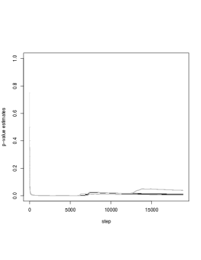
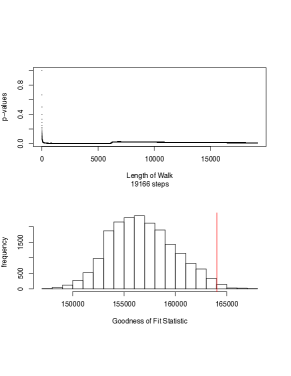
(a) Test of model fit for the dyad-specific $p_{1}$ model on the neuronal chemical (directed) network. Left: $p$-value quartiles for $3$ iterations of the Markov chain. Right: typical $p$-value estimate and the sampling distribution of the goodness-of-fit statistics (chi-square) along with its observed value.

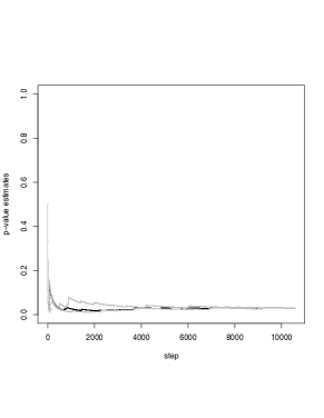
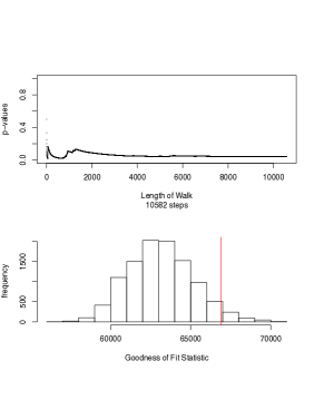
(b) Test of model fit for the dyad-specific $p_{1}$ model on the neuronal electrical (undirected) network. Left: $p$-value quartiles for $5$ iterations of the Markov chain. Right: typical $p$-value estimate and the sampling distribution of the goodness-of-fit statistics (chi-square) along with its observed value.

Figure 2: $p_{1}$ model fit with dyad-specific reciprocation on two neuronal networks.

For the electrical subnetwork of the neuronal network, Figure 2(b) shows the results of testing the $\beta$ model, which is rejected at significance level $>0.04$ (with $p$-values between 0.019 and 0.04 over five iterations of the fit test).

The fact that all four models are rejected with $p$-values often significantly smaller than $0.05$ gives evidence against edge formation based on the attractiveness and expansiveness of the nodes alone, even after taking into account possible reciprocation effects. This supports the observation in Varshney et al. (2011) against a scale-free model of generation and is contrary to scale invariance hypothesis suggested in Towlson et al. (2013).

Next we consider the mixed neuronal network, consisting of the union of the directed graph—the chemical part—and the undirected graph— the gap junction part. Since there are three natural neuron groupings – function, region, and ganglion group – we add a parameter for possible homophily to the $\beta$-model and again test model fit. For the neuronal mixed network we tested the $\beta$-SBM model with block assignments given by each of the three groupings; since the results were the same for all three, we show it for the region group block assignment. Test of model fit of the $\beta$-SBM to the mixed network where the network block assignment is given by blocks = regionBlocks: is illustrated in Figure 3(a). Model rejected at any reasonable significance level, with $p$-value very close to $0$ ($10^{-4}$). Since the $p_{1}$ model naturally interprets undirected edges as reciprocated, testing dyad-specific reciprocation will help delineate the two types of edges. Figure 3(b) shows that this model actually fits the data well; whereas the variant with zero reciprocation does not (the simulation results, similar to the above, are omitted for length considerations.)

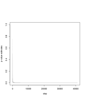
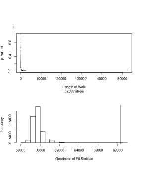
(a) Test of model fit of the $\beta$-SBM model to the neuronal mixed network. Block assignment function is given by RegionBlocks. Left: $p$-value quartiles for $3$ iterations on 200,000 steps each. Right: typical $p$-value estimate from one of the iterations.

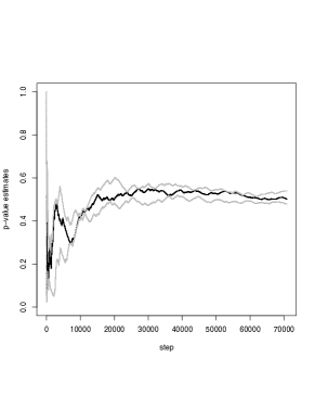
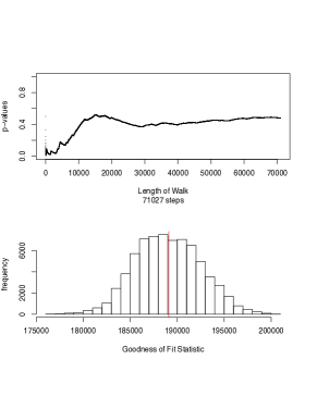
(b) Test of model fit for the $p_{1}$ model with dyad-specific reciprocation effect to the neuronal mixed network consisting of the chemical (undirected) and gap junction (directed) graphs. Left: $p$-value quartiles for $5$ iterations. Right: a typical $p$-value estimate from one of the iterations and the sampling distribution of the goodness-of-fit (chi-square) statistic along with its observed value.

Figure 3: Two models fits on the neuronal mixed network.

As we see in simulation results above, we reject the model for the $p_{1}$-model with zero reciprocation, which again gives evidence against degree-based edge formation. However, for the mixed network under the $p_{1}$-model with dyad specific reciprocation, the model is not rejected. This could be picking up the signal that some neurons are more likely to be a part of electrical connections as opposed to chemical connections, since the electrical connections are represented as reciprocated edges in the mixed network.

4.3 Protein-protein interaction network data

The protein-protein interaction network data set is from Arabidopsis Interactome Mapping Consortium (2011) and available from the Plant Interactome Database (http://interactome.dfci.harvard.edu/A_thaliana/). The data set is the union of two protein-protein interaction graphs which share a subset of proteins as vertices. The first protein-protein interaction graph is a literature-curated network consisting of 3,998 directed interactions on 2,160 proteins. The second protein-protein interaction graph is a partial map of the Arabidopsis thaliana interactome experimentally constructed in Arabidopsis Interactome Mapping Consortium (2011). This second network consists of 2,661 vertices and 5,529 directed edges. The two networks, $G_{1}$ and $G_{2}$ respectively, have 477 proteins in common. We will consider the union of these two directed graphs, which results in a network with $4,344$ vertices and $9,449$ edges. For testing, we will treat edges with one vertex in $V(G_{1})\setminus V(G_{2})$ and the other in $V(G_{2})\setminus V(G_{1})$ (regardless of direction) as structural zeros.

Simulation results.

As with neuronal network, we also test the A. thaliana protein-protein interaction network for evidence of degree-based edge formation. However, if we test the full network with 4,344 vertices and 9,449 edges, there is a large number of edges that we need to treat as structural zeros since these edges were not tested in the experiment. For a data set of this size, that number of structural zeros slows down the algorithm.

Thus, we ran the goodness of fit test after some optimizing, namely, a parallel implementation, small moves tuning parameter that allows to tune the size of move and make the chain ‘move’ faster, etc., and tested the $p_{1}$ model with dyad-specific reciprocation effect, taking into account the structural zeros. Several short simulations completed gave conflicting results, with $p$-values ranging from $0.02$ to $0.2$. Due to the prohibitive computation time, we only ran chains of effective size  20,000 (steps counted disregarding rejected move proposals), arguably insufficient, and did notice that the chains had not mixed yet. A summary of one such run can be seen in Figure 4(a). Figure 4(b) illustrates potential red flags in terms of $p$-value converging: three iterations of the model fit test were run in parallel, and produced different results. A closer look at the simulation reveals that not all the chains have mixed, but the move rejection rate was low.

(a) A 20,000-step Markov chain for the dyad-specific $p_{1}$ model test on the protein-protein interaction network with structural zeros.

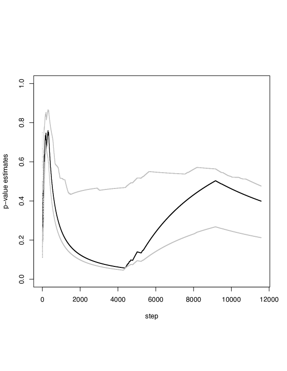
(b) $p$-value convergence for the dyad-specific $p_{1}$ model test on the protein-protein interaction network with structural zeros.

Figure 4: Protein-protein interaction network with a large number of structural zero edges.

We also tested the same model without structural zeros on one of the component graphs and rejected the model after about $15,000$ steps with $p$-values ranging from $0.0005$ to $0.05$.

The reader should note that the prohibitive computation time is not imposed by how our current implementation handles structural zeros or generation of new graphs. Rather, it is a result of other computational issues, such as computing the values of the chi-square statistic at each discovered network. For each new graph generated in the fiber, the chi-square computation requires on the order of a few billion small computations, even though we are using the most optimized version of it. We do not yet have a principled approach to address the challenge of this particular part of the computation to make it more scalable. The reader is referred to the Discussion section for more details.

4.4 Comparison with existing methods

Finally, in this section we compare our results with the goodness-of-fit test implemented in the ergm.R package Hunter et al. (2008a). For comparison, we will restrict our attention to the $\beta$–SBM model. It should be noted that not all models discussed in this paper are implemented in the ergm package, as an example, ergm does not have built in reciprocation terms for the $p_{1}$ model with edge-dependent reciprocation. However, $\beta$–SBM model can be fitted with ergm, and so it is a natural model to use as comparison.

The goodness-of-fit method gof implemented in ergm.R is based on Hunter et al. (2008b). The method gof simulates networks from the fitted model and then computes network statistics of the observed and simulated networks. The method is a graphical test, so to evaluate the goodness-of-fit, the user visually inspects how the distribution of each statistic for the observed network compares with the distributions of the statistic for the simulated networks. Here, using the ergm package, we fit the $\beta$-SBM model to the mixed, undirected neuronal network with blocks assigned according to “region,” and then run gof using the three suggested statistics from Hunter et al. (2008b): degree, edge-wise shared partners, and minimum geodesic distance. The three plots of these statistics are displayed in Figure 5; the black line represents the statistics of the neuronal network, while the grey lines represent the range for 95 percent of the simulated statistics. While the degree statistics of the neuronal network are within the range of the degree statistics of the simulated networks, the edge-wise shared partners and minimum geodesic distances of the neuronal network differ greatly from the simulated networks. Thus using these plots, we conclude that the $\beta$-SBM model is a poor fit for the data, a conclusion supported by §4.2.

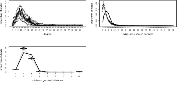
Figure 5: Comparison of degree, edge-wise shared partners, and minimum geodesic distance statistics between simulated networks and the mixed, undirected neuronal network.

We also further experiment with other MCMC algorithms to speed up computations, namely Besag and Clifford’s “parallel method” from Besag and Clifford (1989). In this method, one runs the chain backwards from the observed network $G_{0}$ for a prescribed number of steps to obtain a network $G_{1}$. From $G_{1}$, one then runs $n-1$ independent chains forward to get $n$ simulated random networks that form an approximately independent sample drawn from the uniform distribution on the fiber. While this method worked well for smaller networks, in unoptimized form, it did not scale well for the examples in this paper.

5 Discussion and next steps

The guiding question of this work is how to perform statistically satisfying goodness-of-fit tests for a family of network models with good statistical properties and enough flexibility for broad use in applications. While non-asymptotic tests for general ERGMs remain a generally hard problem, we derive finite-sample tests for model fit for a meaningful subclass of ERGMs called log-linear ERGMs. This is done by importing tools from contingency table analysis and adapting them to the combinatorial setting of random graphs, namely, scalable estimation IPS algorithms and dynamic Markov bases for sampling from conditional distributions. The log-linear setting is a familiar setting for networks and, in particular, this paper is rooted in the connection established in the 1980s by Fienberg and Wasserman (1981b) and Fienberg and Wasserman (1981a).

As an application, we test two popular types of biological datasets in network science, a neuronal network and a protein-protein interaction network. In particular, we test whether the datasets fit several degree-based models, including models with homophily and reciprocation effects. These datasets were chosen since these networks routinely appear as examples of scale-free networks, suggesting degree-based edge formation mechanisms, however, while some authors have suggested exploring biological networks with ERGMs Saul and Filkov (2007), Simpson et al. (2011), up to this point, goodness of fit testing has only been ad hoc. Thus, this work adds not only to the conversation on goodness-of-fit testing for ERGMs, but also to the conversation in network science focused on understanding the general structure of protein-protein interaction networks and neuronal networks. In summary, we rejected most of the models that we fitted to these datasets, with the exception of the $p_{1}$-model with dyad specific reciprocation for the mixed neuronal network containing both the electrical and chemical subnetworks.

The largest network we tested was a protein-protein interaction network with 4,344 nodes and 9,449 edges (see Section 4.3). Testing how well this network fit different variants of the $p_{1}$-model with a large number of structural zeros required a prohibitive, or at least impractical, computation time, which illustrates the limits of the unoptimized way in which we implemented our algorithms in R. One bottleneck in the computation is not the graph sampling, rather, it is that the $\chi^{2}$ statistic is computed at each step in the walk in order to obtain an estimate for the conditional $p$-value. For example, this computation alone requires finding the entry-wise difference between two matrices of size $4344\times 4344=18,870,336$. As fields are moving toward larger and larger datasets, clever computing strategies–or calls to lower-level implementation of such operations–will be needed to handle networks with a million or more nodes. However, we expect there is ample room for improvement by exploiting current research in combinatorial algorithms and the computer science side of data science.

While more work needs to be done to build an efficient algorithm for testing massive networks, the results of this work illustrate the feasibility of straightforward algorithms that utilize Markov bases for medium-sized datasets. In fact, scalability of algorithms that utilize Markov bases have been an open question in the last decade, since such algorithms traditionally rely on pre-computing the entire Markov basis. Such computations are not only time and resource intensive but also produce mostly inapplicable moves since, by definition, these bases are independent of the observed data (Dobra et al., 2008, Problem 5.5); cf. Goldenberg et al. (2009), and are not specialized to any particular fiber of the model. With this issue in mind, various proposals have been made to make exact conditional tests for tables scalable to larger data or more complex models. For example, Dobra (2012) proposes a general dynamic approach to constructing applicable local moves for marginal table models and proves that they can be utilized to cover the entire fiber. Meanwhile, Hara et al. (2012) use a Poisson-size combination of the smallest possible set of moves to explore fibers of discrete logistic regression models, and Martin del Campo et al. (2017) use another small subset of a Markov basis for testing the Ising model on a large biological dataset. Each of these methods extends the use of Markov bases to larger and larger datasets: the approach in Dobra (2012) was demonstrated on tables up to 256 cells, Hara et al. (2012) show their method approaches its limits on $10\times 10\times 10$ tables, and Martin del Campo et al. (2017) are able to use their method on a biological dataset of size $800\times 800$. In this paper, we are able to obtain good results for tables up of size $2661\times 2661\times 2\times 2$ (networks with 2661 vertices) and show that our method slows down due to a goodness-of-fit statistic computation on tables of size $4334\times 4334\times 2\times 2$ (networks with 4334 vertices).

One immediate benefit of using a contingency table representation and Markov bases is the ease of generalization of the goodness of fit test to models for multi-graphs, that is, graphs with positive integer weights on the edges. This can be achieved by simply removing the $0/1$ table entry sampling restriction; the resulting estimation algorithms are not affected, and the sampling algorithms based on Markov bases, in fact, become simpler because they do not require the additional step of checking for the graph being simple. Due to this simplification, we expect the sampling algorithm’s mixing time and scalability to improve in this setting. In regards to the mixing time of the proposed algorithms in this manuscript, we note that Dillon (2016) showed that the dynamic Markov bases algorithm from Gross et al. (2016) is rapidly mixing on many fibers, since it contains the simple switch chain well-known in the graph theory literature Kannan et al. (1999b). Although herein we propose many more chains than Gross et al. (2016), most of these chains also contain the simple switch chain, which provides ample evidence that the algorithms will mix rapidly on most fibers, even if a formal mixing time analysis is outside the scope of this paper.

On a final note, if it is known that the data does not support dyadic independence, analysis using more complicated ERGMs outside of the log-linear ERGM class would be desirable, though tests of model fit is a looming question. In such cases, the sufficient statistic is no longer linear in terms of the dyads, and the geometry and combinatorics of the fibers of the resulting model (that is, graphs with the fixed value of the sufficient statistic) is poorly understood. While there exist models that do not assume dyadic independence, ranging from the very simple edge-triangle model Strauss (1986); Park and Newman (2004, 2005) to those using global summary statistics Karwa et al. (2017), it is not clear how to use any available tools for testing the dyadic independence assumption on a given network from a statistical point of view. One may turn to estimating graphical models on dyads such as Frank and Strauss (1986) or more recent general models from Sadeghi and Rinaldo (2020), however for these models, testing goodness of fit is an open problem as well.

Appendix A Parameter hypergraphs

In this appendix, we define and give several examples of a combinatorial structure that encodes any log-linear model: the parameter hypergraph. One should think of this discrete structure object as a schematic representation of the model parametrization, as it encodes the way in which parameters of the model interact. For example in the $\beta$-model, log-odds of each edge probability $p_{ij}$, $\beta_{i}+\beta_{j}$, is encoded by grouping the two parameters $\{\beta_{i},\beta_{j}\}$ together. Each such set represents one edge in the parameter hypergraph. In mathematically precise terms, a hypergraph $\mathcal{H}=(\mathcal{V},\mathcal{E})$ is an ordered pair where $\mathcal{V}$ is a set of elements called vertices and $\mathcal{E}$ is a set of non-empty subsets of $\mathcal{V}$ called hyperedges, or simply edges. Note that a graph is an instance of a hypergraph where all edges are subsets of $\mathcal{V}$ of size 2.

The general setup is that the vertices of the parameter hypergraph are the model parameters, while the edges are sets of parameters that appear together in any one of edge probability (or, equivalently, their log-odds). In particular, the edge sets for the degree-based models below should be compared to the equations in Section 2.1.

A.1 Combinatorics of $\beta$-model

The parameter hypergraph $\mathcal{H}=(\mathcal{V},\mathcal{E})$ of the $\beta$-model on $\mathcal{G}_{n}$ has vertex set

$$\mathcal{V}=\{\beta_{i}\ :\ 1\leq i\leq n\}$$

and edge set

$$\mathcal{E}=\{\{\beta_{i},\beta_{j}\}\ :\ 1\leq i<j\leq n\}.$$

Notice that for the $\beta$-model, the parameter hypergraph is the complete graph on $n$ vertices.

A.2 Combinatorics of the $p_{1}$ model with zero reciprocation

The parameter hypergraph of the $p_{1}$-model with zero reciprocation on $\mathcal{G}_{n}$ is $\mathcal{H}=(\mathcal{V},\mathcal{E})$ where

$$\mathcal{V}=\{\alpha_{i},\ \beta_{j}\ :\ 1\leq i\leq n,\ 1\leq j\leq n\}\text{ and }\mathcal{E}=\{\{\alpha_{i},\beta_{j}\}\ :\ 1\leq i,j\leq n,\ i\neq j\}.$$

Notice that by restricting to the edges of size two in $\mathcal{E}$, we obtain the complete bipartite graph $K_{n,n}$ with the edges $\{\alpha_{i},\beta_{i}\}$ removed.

A careful reader may notice the absence of the parameters $\lambda_{ij}$. These are normalizers added to the model parametrization in order to ensure that each dyad is observed in exactly one of the four states. From a combinatorial point of view, they add complexity to the hypergraph, but do not change the underlying structure from which Markov moves for sampling are derived. So it is simpler to not include them in the structural consideration.

A.3 Combinatorics of the $p_{1}$ model with constant reciprocation

The parameter hypergraph of the $p_{1}$-model with constant reciprocation on $\mathcal{G}_{n}$ is $\mathcal{H}=(\mathcal{V},\mathcal{E})$ where

$$\mathcal{V}=\{\alpha_{i},\ \beta_{j},\rho\ :\ 1\leq i\leq n,\ 1\leq j\leq n\}\text{ and }\mathcal{E}=\{\{\alpha_{i},\beta_{j}\},\{\alpha_{i},\alpha_{j},\beta_{i},\beta_{j},\rho\}\ :\ 1\leq i,j\leq n,\ i\neq j\}.$$

Notice that, as in the zero reciprocation case, by restricting to the edges of size two in $\mathcal{E}$, we obtain the complete bipartite graph $K_{n,n}$ with the edges $\{\alpha_{i},\beta_{i}\}$ removed.

A.4 Combinatorics of the $p_{1}$ model with dyad-specific reciprocation

The parameter hypergraph of the $p_{1}$-model with constant reciprocation on $\mathcal{G}_{n}$ is $\mathcal{H}=(\mathcal{V},\mathcal{E})$ where

$$\mathcal{V}=\{\alpha_{i},\ \beta_{j},\rho\ :\ 1\leq i\leq n,\ 1\leq j\leq n\}\text{ and }\mathcal{E}=\{\{\alpha_{i},\beta_{j}\},\{\alpha_{i},\alpha_{j},\beta_{i},\beta_{j},\rho_{i},\rho_{j}\}\ :\ 1\leq i,j\leq n,\ i\neq j\}.$$

As in the previous two $p_{1}$ models, restricting to the edges of size two in $\mathcal{E}$, we obtain the complete bipartite graph $K_{n,n}$ with the edges $\{\alpha_{i},\beta_{i}\}$ removed. Additionally, notice the induced hypergraph on $\mathcal{V}_{\rho}=\{\rho_{i}\ :\ 1\leq i\leq n\}$ gives us the complete graph on $n$ vertices.

Appendix B The conversion step

Step 2 of Algorithm 2 is a subroutine to convert a dyad classification table $v$ to a multihypergraph $\mathbb{R}$. The log-linear model matrix $A$ is the incidence model of the parameter hypergraph, so rows of $A$ are indexed by vertices (model parameters), and columns are indexed by dyads. There are as many columns of $A$ as there are cells in the dyadic classification table $u$ of a network $g$.

The conversion then is as follows. Each nonzero entry in a cell $e$ of a given subtable $v$ is encoded as an edge of the parameter graph corresponding to the column $A_{e}$.

In the example from A.3, an entry $m\in\mathbb{Z}_{\geq 0}$ in the cell representing the dyad $\{i,j\}$ in state $i\leftrightarrow j$ is converted into $m$ copies of the hyperedge $\{\alpha_{i}\beta_{j}\}$. Entry $m$ in the cell representing the dyad $\{i,j\}$ in the state $i\leftrightarrow j$ is converted into $m$ copies of the hyperedge $\{\alpha_{i}\beta_{j}\rho\}$.

References

- Achacoso and Yamamoto (1992) Achacoso, T. and Yamamoto, W. (1992). AY’s Neuroanatomy of C. elegans for Computation. CRC Press.
- Admiraal and Handcock (2008) Admiraal, R. N. and Handcock, M. S. (2008). networksis: A package to simulate bipartite graphs with fixed marginals through sequential importance sampling. Journal of Statistical Software, 24(8).
- Albert (2005) Albert, R. (2005). Scale-free networks in cell biology. Journal of cell science, 118(21), 4947–4957.
- Anderson et al. (1999) Anderson, B. S., Butts, C., and Carley, K. (1999). The interaction of size and density with graph-level indices. Social networks, 21(3), 239–267.
- Aoki et al. (2012) Aoki, S., Hara, H., and Takemura, A. (2012). Markov bases in algebraic statistics, volume 199. Springer Science & Business Media.
- Arabidopsis Interactome Mapping Consortium (2011) Arabidopsis Interactome Mapping Consortium (2011). Evidence for network evolution in an arabidopsis interactome map. Science, 333(6042), 601–607.
- Banerjee and Ma (2017) Banerjee, D. and Ma, Z. (2017). Optimal hypothesis testing for stochastic block models with growing degrees. ArXiv, abs/1705.05305.
- Barucca and Lillo (2016) Barucca, P. and Lillo, F. (2016). Disentangling bipartite and core-periphery structure in financial networks. Chaos, Solitons & Fractals, 88, 244–253.
- Bentley et al. (2016) Bentley, B., Branicky, R., Barnes, C. L., Chew, Y. L., Yemini, E., Bullmore, E. T., Vértes, P. E., and Schafer, W. R. (2016). The multilayer connectome of caenorhabditis elegans. PLOS Computational Biology, 12(12), 1–31.
- Besag and Clifford (1989) Besag, J. and Clifford, P. (1989). Generalized Monte Carlo significance tests. Biometrika, 76(4), 633–642.
- Bishop and Fienberg (2007) Bishop, Y. M. and Fienberg, S. E. (2007). Discrete multivariate analysis theory and practice.
- Blitzstein and Diaconis (2010) Blitzstein, J. and Diaconis, P. (2010). A sequential importance sampling algorithm for generating random graphs with prescribed degrees. Internet Math, 6, 489–522.
- Breiger (1981) Breiger, R. L. (1981). An exponential family of probability distributions for directed graphs: Comment. Journal of the American Statistical Association, 76(373), 51–53.
- Cabreros et al. (2016) Cabreros, I., Abbe, E., and Tsirigos, A. (2016). Detecting community structures in hi-c genomic data. In 2016 Annual Conference on Information Science and Systems (CISS), pages 584–589. IEEE.
- Carnegie et al. (2015) Carnegie, N. B., Krivitsky, P. N., Hunter, D. R., and Goodreau, S. M. (2015). An approximation method for improving dynamic network model fitting. Journal of Computational and Graphical Statistics, 24(2), 502–519.
- Chatterjee and Diaconis (2013) Chatterjee, S. and Diaconis, P. (2013). Estimating and understanding exponential random graph models. The Annals of Statistics, 41(5), 2428–2461.
- Chatterjee et al. (2011) Chatterjee, S., Diaconis, P., and Sly, A. (2011). Random graphs with a given degree sequence. Annals of Applied Probability, 21(4), 1400–1435.
- Choi et al. (2011) Choi, D. S., Wolfe, P., and Airoldi, E. M. (2011). Confidence sets for network structure. In Advances in Nueral Information Processing Systems, volume 24. NIPS 2011.
- Clauset et al. (2009) Clauset, A., Shalizi, C. R., and Newman, M. E. (2009). Power-law distributions in empirical data. SIAM review, 51(4), 661–703.
- Diaconis and Sturmfels (1998) Diaconis, P. and Sturmfels, B. (1998). Algebraic algorithms for sampling from conditional distribution. Annals of Statistics, 26(1), 363–397.
- Dillon (2016) Dillon, M. (2016). Runtime for performing exact tests on the statistical model for random graphs, MS thesis.
- Dobra (2012) Dobra, A. (2012). Dynamic Markov bases. Journal of Computational and Graphical Statistics, pages 496–517.
- Dobra et al. (2008) Dobra, A., Fienberg, S. E., Rinaldo, A., Slavković, A., and Zhou, Y. (2008). Algebraic statistics and contingency table problems: Log-linear models, likelihood estimation and disclosure limitation. In IMA Volumes in Mathematics and its Applications: Emerging Applications of Algebraic Geometry, pages 63–88. Springer Science+Business Media, Inc.
- Drton et al. (2009) Drton, M., Sturmfels, B., and Sullivant, S. (2009). Lectures on Algebraic Statistics, volume 39 of Oberwolfach Seminars. Springer, Basel.
- Erdős et al. (2015) Erdős, P. L., Kiss, S. Z., Miklós, I., and Soukup, L. (2015). Approximate counting of graphical realizations. PloS one, 10(7), e0131300.
- Fienberg and Rinaldo (2012) Fienberg, S. E. and Rinaldo, A. (2012). Maximum likelihood estimation in log-linear models. Annals of Statistics, 40, 996–1023.
- Fienberg and Wasserman (1981a) Fienberg, S. E. and Wasserman, S. S. (1981a). Categorical data analysis of single sociometric relations. Sociological methodology, 12, 156–192.
- Fienberg and Wasserman (1981b) Fienberg, S. E. and Wasserman, S. S. (1981b). Discussion of Holland, P. W. and Leinhardt, S. “An exponential family of probability distributions for directed graphs”. Journal of the American Statistical Association, 76, 54–57.
- Fienberg et al. (1985) Fienberg, S. E., Meyer, M. M., and Wasserman, S. S. (1985). Statistical analysis of multiple sociometric relations. Journal of the American Statistical Association, 80(389), 51–67.
- Fienberg et al. (2010) Fienberg, S. E., Petrović, S., and Rinaldo, A. (2010). Algebraic statistics for random graph models: Markov bases and their uses, volume Papers in Honor of Paul W. Holland, ETS. Springer.
- Frank and Strauss (1986) Frank, O. and Strauss, D. (1986). Markov graphs. Journal of the American Statistical Association, 81(395), 832–842.
- Funke and Becker (2019) Funke, T. and Becker, T. (2019). Stochastic block models: A comparison of variants and inference methods. PloS one, 14(4), e0215296.
- Geiger et al. (2006) Geiger, D., Meek, C., and Sturmfels, B. (2006). On the toric algebra of graphical models. https://arxiv.org/abs/math/0608054.
- Goldenberg et al. (2009) Goldenberg, A., Zheng, A. X., Fienberg, S. E., and Airoldi, E. M. (2009). A survey of statistical network models. Foundations and Trends in Machine Learning, 2(2), 129–233.
- Gross et al. (2016) Gross, E., Petrović, S., and Stasi, D. (2016). Goodness of fit for log-linear network models: Dynamic Markov bases using hypergraphs. Annals of the Institute of Statistical Mathematics. DOI: 10.1007/s10463-016-0560-2.
- Gross et al. (2022) Gross, E., Petrović, S., and Karwa, V. (2022). Algebraic statistics, tables, and networks: The Fienberg advantage. In A. L. Carriquiry, J. M. Tanur, and W. F. Eddy, editors, Statistics in the Public Interest: In Memory of Stephen E. Fienberg. Springer International Publishing.
- Handcock (2003) Handcock, M. S. (2003). Assessing degeneracy in statistical models of social networks. CSSS Working paper #39.
- Hara and Takemura (2010) Hara, H. and Takemura, A. (2010). Connecting tables with zero-one entries by a subset of a markov basis. In M. Viana and H. Wynn, editors, Algebraic Methods in Statistics and Probability II, volume 516 of Contemporary Mathematics. American Mathematical Society.
- Hara et al. (2012) Hara, H., Aoki, S., and Takemura, A. (2012). Running Markov chain without Markov basis. In T. Hibi, editor, Harmony of Gröbner Bases and the Modern Industrial Society. World Scientific.
- Holland and Leinhardt (1981) Holland, P. W. and Leinhardt, S. (1981). An exponential family of probability distributions for directed graphs (with discussion). Journal of the American Statistical Association, 76(373), 33–65.
- Holland et al. (1983) Holland, P. W., Laskey, K. B., and Leinhardt, S. (1983). Stochastic blockmodels: First steps. Social networks, 5(2), 109–137.
- Hunter et al. (2008a) Hunter, D. R., Handcock, M. S., Butts, C. T., Goodreau, S. M., and Morris, M. (2008a). ergm: A package to fit, simulate and diagnose exponential-family models for networks. Journal of Statistical Software, 24(3), 1–29.
- Hunter et al. (2008b) Hunter, D. R., Goodreau, S. M., and Handcock, M. S. (2008b). Goodness of fit of social network models. Journal of the American Statistical Association, 103(481), 248–258.
- Jeong et al. (2000) Jeong, H., Tombor, B., Albert, R., Oltvai, Z. N., and Barabási, A.-L. (2000). The large-scale organization of metabolic networks. Nature, 407(6804), 651–654.
- Kannan et al. (1999a) Kannan, R., Tetali, P., and Vempala, S. (1999a). Simple markov-chain algorithms for generating bipartite graphs and tournaments. Random Structures & Algorithms, 14(4), 293–308.
- Kannan et al. (1999b) Kannan, R., Tetali, P., and Vempala, S. (1999b). Simple Markov-chain algorithms for generating bipartite graphs and tournaments. Random Structures and Algorithms, 14(1), 293–308.
- Karrer and Newman (2011) Karrer, B. and Newman, M. E. (2011). Stochastic blockmodels and community structure in networks. Physical Review E, 83(1), 016107.
- Karwa et al. (2016) Karwa, V., Pati, D., Petrović, S., Solus, L., Alexeev, N., Raič, M., Wilburne, D., Williams, R., and Yan, B. (2016). Monte Carlo goodness-of-fit tests for degree corrected and related stochastic blockmodels. arXiv preprint arXiv:1612.06040.
- Karwa et al. (2017) Karwa, V., Pelsmajer, M., Petrović, S., Stasi, D., and Wilburne, D. (2017). Statistical models for cores decomposition of an undirected random graph. Electronic Journal of Statistics, 11(1), 1949–1982.
- Kim et al. (2012) Kim, H., Del Genio, C. I., Bassler, K. E., and Toroczkai, Z. (2012). Constructing and sampling directed graphs with given degree sequences. New Journal of Physics, 14(2), 023012.
- Kolaczyk (2017) Kolaczyk, E. D. (2017). Topics at the Frontier of Statistics and Network Analysis: (Re)Visiting the Foundations. Cambridge University Press.
- Lee and Wilkinson (2019) Lee, C. and Wilkinson, D. J. (2019). A review of stochastic block models and extensions for graph clustering. Applied Network Science, 4(1), 1–50.
- Lei (2016) Lei, J. (2016). A goodness-of-fit test for stochastic block models. Annals of Statistics.
- Martin del Campo et al. (2017) Martin del Campo, A., Cepeda, S., and Uhler, C. (2017). Exact goodness-of-fit testing for the ising model. Scandinavian Journal of Statistics, 44(2), 285–306.
- Moreno (1934) Moreno, J. (1934). Who shall survive?: A new approach to the problem of human interrelations. Nervous and Mental Disease Publishing Co, https://doi.org/10.1037/10648-000.
- Nowicki and Snijders (2001) Nowicki, K. and Snijders, T. A. B. (2001). Estimation and prediction for stochastic blockstructures. Journal of the American Statistical Association, 96(455), 1077–1087.
- Ogawa et al. (2013) Ogawa, M., Hara, H., and Takemura, A. (2013). Graver basis for an undirected graph and its application to testing the beta model of random graphs. Annals of Institute of Statistical Mathematics, 65(1), 191–212.
- Park and Newman (2004) Park, J. and Newman, M. E. J. (2004). Solution of the two-star model of a network. Physical Review E, 70(3), 066146.
- Park and Newman (2005) Park, J. and Newman, M. E. J. (2005). Solution for the properties of a clustered network. Physical Review E, 72(3), 026136.
- Pattison and Wasserman (1999) Pattison, P. and Wasserman, S. (1999). Logit models and logistic regressions for social networks: II. multivariate relations. British Journal of Mathematical and Statistical Psychology, 52(2), 169–193.
- Pavlovic et al. (2014) Pavlovic, D. M., Vértes, P. E., Bullmore, E. T., Schafer, W. R., and Nichols, T. E. (2014). Stochastic blockmodeling of the modules and core of the caenorhabditis elegans connectome. PloS one, 9(7), e97584.
- Petrović and Stasi (2014) Petrović, S. and Stasi, D. (2014). Toric algebra of hypergraphs. Journal of Algebraic Combinatorics, 39(1), 187–208.
- Petrović et al. (2010) Petrović, S., Rinaldo, A., and Fienberg, S. E. (2010). Algebraic statistics for a directed random graph model with reciprocation. In M. Viana and H. Wynn, editors, Algebraic Methods in Statistics and Probability II, volume 516 of Contemporary Mathematics, pages 261–283. American Mathematical Society, Providence RI.
- Rao et al. (1996) Rao, A. R., Jana, R., and Bandyopadhyay, S. (1996). A Markov chain Monte Carlo method for generating random (0, 1)-matrices with given marginals. Sankhyā: The Indian Journal of Statistics, Series A, pages 225–242.
- Rinaldo et al. (2013) Rinaldo, A., Petrović, S., and Fienberg, S. E. (2013). Maximum likelihood estimation in the Beta model. Annals of Statistics, 41(3), 1085–1110.
- Robert and Casella (1999) Robert, C. and Casella, G. (1999). Monte Carlo Statistical Methods. Springer Texts in Statistics. Springer-Verlag, New York.
- Robins et al. (1999) Robins, G., Pattison, P., and Wasserman, S. (1999). Logit models and logistic regressions for social networks: III. valued relations. Psychometrika, 64(3), 371–394.
- Robins et al. (2007) Robins, G., Pattison, P., Kalish, Y., and Lusher, D. (2007). An introduction to exponential random graph (p*) models for social networks. Social networks, 29(2), 173–191.
- Ryser (1987) Ryser, H. (1987). Combinatorial properties of matrices of zeros and ones. Classic Papers in Combinatorics, pages 269–275.
- Sadeghi and Rinaldo (2020) Sadeghi, K. and Rinaldo, A. (2020). Hierarchical models for independence structures of networks. Statistica Neerlandica, Netherlands Society for Statistics and Operations Research, 74(3), 439–457. Preprint. arXiv:1605.04565.
- Saul and Filkov (2007) Saul, Z. M. and Filkov, V. (2007). Exploring biological network structure using exponential random graph models. Bioinformatics, 23(19), 2604–2611.
- Schweinberger et al. (2020) Schweinberger, M., Krivitsky, P., Butts, C., and Stewart, J. (2020). Exponential-family models of random graphs: Inference in finite, super, and infinite population scenarios. Statistical Science, 35, 627–662.
- Shalizi and Rinaldo (2013) Shalizi, C. R. and Rinaldo, A. (2013). Consistency under sampling of exponential random graph models. Annals of Statistics, 41(2), 508.
- Simpson et al. (2011) Simpson, S. L., Hayasaka, S., and Laurienti, P. J. (2011). Exponential random graph modeling for complex brain networks. PloS one, 6(5), e20039.
- Strauss (1986) Strauss, D. (1986). On a general class of models for interaction. SIAM review, 28, 513–527.
- Sturmfels (1996) Sturmfels, B. (1996). Gröbner bases and convex polytopes. University Lecture Series, no. 8, American Mathematical Society.
- Tabourier et al. (2011) Tabourier, L., Roth, C., and Cointet, J.-P. (2011). Generating constrained random graphs using multiple edge switches. Journal of Experimental Algorithmics (JEA), 16, 1–7.
- Tanaka (2005) Tanaka, R. (2005). Scale-rich metabolic networks. Physical review letters, 94(16), 168101.
- Taylor (1981) Taylor, R. (1981). Contrained switchings in graphs. In Combinatorial Mathematics VIII, pages 314–336. Springer.
- Towlson et al. (2013) Towlson, E. K., Vértes, P. E., Ahnert, S. E., Schafer, W. R., and Bullmore, E. T. (2013). The rich club of the c. elegans neuronal connectome. Journal of Neuroscience, 33(15), 6380–6387.
- Varshney et al. (2011) Varshney, L. R., Chen, B. L., Paniagua, E., Hall, D. H., and Chklovskii, D. B. (2011). Structural properties of the caenorhabditis elegans neuronal network. PLoS Computational Biology, 7(2).
- Wagner and Fell (2001) Wagner, A. and Fell, D. A. (2001). The small world inside large metabolic networks. Proceedings of the Royal Society of London B: Biological Sciences, 268(1478), 1803–1810.
- Wang (2020) Wang, G. (2020). A fast mcmc algorithm for the uniform sampling of binary matrices with fixed margins. Electronic Journal of Statistics, 14, 1690–1706.
- Wasserman and Pattison (1996) Wasserman, S. and Pattison, P. (1996). Logit models and logistic regressions for social networks: I. an introduction to Markov graphs and. Psychometrika, 61(3), 401–425.
- Watts and Strogatz (1998) Watts, D. J. and Strogatz, S. H. (1998). Collective dynamics of ’small-world’ networks. Nature, 393, 440–442.
- Yan et al. (2019) Yan, T., Jiang, B., Fienberg, S. E., and Leng, C. (2019). Statistical inference in a directed network model with covariates. Journal of the American Statistical Association, 114(526), 857–868.
- Yang (2015) Yang, X. (2015). Social Network Modeling and the Evaluation of Structural Similarity for Community Detection. Ph.D. thesis, Carnegie Mellon University.
- Zhang and Chen (2013) Zhang, J. and Chen, Y. (2013). Sampling for conditional inference on network data. Journal of the American Statistical Association, 108(403).