S stars and s-process in the Gaia era

Abstract

Context. S stars are late-type giants that are transition objects between M-type stars and carbon stars on the asymptotic giant branch (AGB). They are classified into two types: intrinsic or extrinsic, based on the presence or absence of technetium (Tc). The Tc-rich or intrinsic S stars are thermally-pulsing (TP-)AGB stars internally producing s-process elements (including Tc) which are brought to their surface via the third dredge-up (TDU). Tc-poor or extrinsic S stars gained their s-process overabundances via accretion of s-process-rich material from an AGB companion which has since turned into a dim white dwarf.

Aims. Our goal is to investigate the evolutionary status of Tc-rich S stars by locating them in a Hertzsprung-Russell (HR) diagram using the results of Gaia early Data Release 3 (EDR3). We combine the current sample of 13 Tc-rich stars with our previous studies of 10 Tc-rich stars to determine the observational onset of the TDU in the metallicity range [-0.7; 0]. We also compare our abundance determinations with dedicated AGB nucleosynthesis predictions.

Methods. The stellar parameters are derived using an iterative tool which combines HERMES high-resolution spectra, accurate Gaia EDR3 parallaxes, stellar evolution models and tailored MARCS model atmospheres for S-type stars. Using these stellar parameters we determine the heavy-element abundances by line synthesis.

Results. In the HR diagram, the intrinsic S stars are located at higher luminosities than the predicted onset of the TDU. These findings are consistent with Tc-rich S stars being genuinely TP-AGB stars. The comparison of the derived s-process abundance profiles of our intrinsic S stars with the nucleosynthesis predictions provide an overall good agreement. Stars with highest [s/Fe] tend to have the highest C/O ratios.

1 Introduction

S stars are late-type giants displaying, as the most characteristic feature of their optical spectra, ZrO bands (Merrill, 1922) along with the usual TiO bands present in stars of similar temperatures (approximately 3000-4000 K, as M-type stars). The spectra show overabundances of s-process elements (Smith & Lambert, 1990) produced by the slow capture of neutrons on elements heavier than Fe (Burbidge et al., 1957; Käppeler et al., 2011) during the thermally-pulsing AGB phase (TP-AGB). These elements are then brought to the surface of the AGB star through mixing processes called third dredge-ups (TDU). The carbon over oxygen (C/O) ratio of S stars is in the range 0.5 to 0.99 which makes them transition objects between M-type (C/O $\sim$ 0.4) and carbon (C/O ¿1) stars (Iben & Renzini, 1983).

Another important characteristic of the S star family is the technetium (Tc) dichotomy. Tc is an element produced by the s-process and which has no stable isotope. Its isotope ⁹⁹Tc has a half-life of 210 000 yrs. The puzzling detection of Tc in some S stars but not in others was solved after realizing that the S stars without Tc (i.e. Tc-poor S stars) belong to binary systems. They are called extrinsic S stars (Smith & Lambert, 1988; Jorissen et al., 1993) because they owe their s-process abundances to mass transfer from a former AGB companion which is now a white dwarf. Therefore, the extrinsic S stars show s-process overabundances, except for Tc, which has decayed since the termination of the AGB phase of the companion. On the contrary, Tc-rich S stars, called intrinsic, are producing s-process elements including Tc and transporting them to their surface via ongoing, recurrent TDU episodes.

We recently discovered a third class of S stars, the bitrinsic S stars (Shetye et al., 2020, S20 hereafter) that share properties with both the intrinsic and extrinsic classes: they are Tc-rich and as such are located on the TP-AGB, but they also show overabundances of Nb, a signature of extrinsically-enriched stars (Neyskens et al., 2015; Shetye et al., 2018; Karinkuzhi et al., 2018). Indeed, the unstable ⁹³Zr isotope (produced by the s-process) decays into ⁹³Nb, the only stable isotope of Nb, in 1.53 Myr. Therefore a niobium enrichment is expected in extrinsic stars, while it is not in TP-AGB stars.

The intrinsic S stars play an important role in our understanding of AGB nucleosynthesis and in particular of the TDU. They are the first objects on the AGB to show clear signatures (Tc and ZrO) of the TDU occurrences. They constrain the minimum luminosity of the TDU as well as its mass and metallicity dependence. The recent discovery of intrinsic, low-mass (initial mass ¡ 1.5 M_⊙), solar metallicity S stars (Shetye et al., 2019, S19 hereafter) provided an observational evidence of the operation of TDUs even in low-mass stars.

In a previous paper (Shetye et al., 2018, S18 hereafter) we introduced a new method for the parameter and abundance determination in S-type stars. However, the number of intrinsic S stars available at the time of that study was limited by the bias of the Tycho-Gaia astrometric solution against extremely red sources (Michalik et al., 2015). In the current work we investigate the chemical composition and evolutionary status of 13 intrinsic S stars from Gaia DR2 for which we could obtain high-resolution spectra. This paper is a follow up on the investigation of the evolutionary status of S stars conducted in the pioneering work of Smith & Lambert (1990). We introduce the observational sample in Section 2 and discuss the Tc detection in Section 3. Sections 4 and 5 are dedicated to the description of the parameter and abundance determination. In Section 6 we present the Gaia EDR3 HR diagram of intrinsic and extrinsic S stars. We discuss the derived elemental abundances of the sample stars and compare them with nucleosynthesis predictions in Section 7. Finally, we conclude with a summary of the most important results.

2 Observational sample

From the General Catalogue of Galactic S-Stars (Stephenson, 1984, CGSS), we selected the ones with a Gaia Data Release 2 (DR2) parallax matching the condition $\sigma_{\varpi}/\varpi$ $\leq 0.3$ and with available HERMES high-resolution spectra (Raskin et al., 2011). From this sample we distinguished the intrinsic S stars from the extrinsic ones using Tc lines (Section 3) and kept only the Tc-rich S stars. Among these, the Tc-rich S stars with initial masses smaller than 1.5 M_⊙ were studied in S19. The cases of BD +79^∘156 and $o^{1}$ Ori, two bitrinsic stars, were discussed in S20. In the current work we derive parameters and abundances for the remaining Tc-rich S stars and also compile the Tc-rich S star results from S18 (3 stars), S19 (5 stars), S20 (2 stars) to increase the size of our sample.

Though the sample was designed using the Gaia DR2, Gaia early Data Release 3 (EDR3) became public during the course of our analysis. Hence the stellar parameters and luminosities were derived using Gaia EDR3. The relative parallax difference between the two releases $|\varpi_{\rm DR2}-\varpi_{\rm EDR3}|/\varpi_{\rm EDR3}$ is usually smaller than 12% (except for V812 Oph, CSS 151, and CSS 454 which show the largest relative deviations of 22%, 33% and 57.5%, respectively). The cause of the large parallax difference of some stars between DR2 and EDR3 is not yet clear. However, to make a consistent comparison of the present study with the previously studied samples (S18, S19 and S20), we re-computed the luminosities of all the extrinsic and intrinsic stars of S18, S19 and S20 using EDR3 (Table 12). As a result, some stars previously identified (using DR2 parallaxes) as low-mass S stars (BD +34^∘ 1698 = CSS 413 and HD 357941 = CSS 1190; see S19) turn out to have higher masses (M_ini = 1.4 and 3.5 M_⊙ respectively) according to their location in the HR diagram using EDR3 parallaxes (Sect. 6). This change in their masses required to adopt a $\log g$ value different from the one used for their abundance analysis in S19 (both stars had $\log g$ $\sim$ 1 in S19; with EDR3 we find instead $\log g$ $\sim$ 0 for both of them). Hence, in the current work we also re-computed the stellar parameters and abundances of BD +34^∘1698 and HD 357941, along the guidelines described in Sections. 4 and 5 using the EDR3 parallaxes (Table 13).

A last criterion to define the Tc-rich S-star sample relates to the photometric variability. Large convective cells and/or pulsations are responsible for the photometric variability of TP-AGB stars. The thermal structure of these pulsating atmospheres can be significantly different from time-independent, hydrostatic atmospheres used to derive their stellar parameters, which can therefore be quite unreliable. We checked the time series data obtained by the American Association of Variable Star Observers (AAVSO) and removed from our sample the Tc-rich S stars with photometric variability $\Delta V>$ 1 mag (see Table 1) except for V812 Oph. The HERMES spectra of V812 Oph, despite its high variability ($\Delta V>$ 1.4 mag), matched well the atmospheric models all over the optical range, hence we included it in the current sample. The sample of newly analyzed stars is listed in Table 2.

Table 1: The Tc-rich S stars excluded from the current study because of their large photometric variability.

CGSS	AAVSO	$\Delta V$ (mag)
9	0018 + 38	7.65
307	0701 + 22	7.53
347	0720 + 46	1.39
856	1425 + 84	2.95
1219	2023 + 36	1.10
1115	1910 - 07	4.76
1309	2245 +17	4.74

Table 2: Basic data for our S star sample.

CSS	Name	Sp. type	$V$	$K$	$J$	$\varpi_{\rm EDR3}\pm\sigma_{\varpi}$	$Z_{5}$	$E_{B-V}$	$BC_{K}$	Observation date	S/N
						(mas)	(mas)
89	V1139 Tau	S	7.90	0.97	2.27	1.79 $\pm$ 0.05	-0.047	0.34	3.00	23 November 2012	150
151	CSS 151	S	10.99	4.64	5.97	0.36 $\pm$ 0.03	-0.053	0.27	2.91	31 July 2017	40
233	HD 288833	S3/2	9.40	4.26	5.51	0.83 $\pm$ 0.02	-0.038	0.31	2.84	20 August 2012	100
265	KR CMa	M4S	8.50	1.96	3.30	1.29 $\pm$ 0.03	-0.030	0.11	3.01	10 April 2011	70
312	AA Cam	M5S	7.79	1.39	2.59	2.08 $\pm$ 0.05	-0.024	0.13	2.84	9 April 2011	90
416	HD 64147	S5/2.5	9.20	3.61	5.00	0.56 $\pm$ 0.03	-0.041	0.09	2.93	27 November 2016	40
454	CSS 454	S	10.39	4.93	6.13	0.40 $\pm$ 0.03	-0.045	0.07	2.91	2 February 2017	50
474	CD -27∘5131	S4,2	9.62	2.72	4.35	0.64 $\pm$ 0.03	-0.031	0.14	3.01	2 April 2010	70
597	BD -18∘2608	S	9.58	4.01	5.27	0.71 $\pm$ 0.02	-0.038	0.14	2.91	24 March 2018	70
997	V812 Oph	S5+/2.5	10.58	4.00	5.22	0.64 $\pm$ 0.03	-0.053	0.22	2.93	22 April 2016	40
1070	V679 Oph	S5/5+	8.92	2.69	4.16	1.04 $\pm$ 0.03	-0.049	0.37	2.83	16 March 2018	80
1152	Vy 12	S5-/6	10.13	3.76	5.06	0.58 $\pm$ 0.02	-0.037	0.21	2.99	18 March 2018	80
1315	HR Peg	S4+/1+	6.36	0.94	2.15	2.14 $\pm$ 0.08	-0.043	0.12	2.93	17 July 2009	60

3 Tc detection

Three Tc I resonance lines located at 4238.19, 4262.27 and 4297.06 Å were used. A signal to noise ratio (S/N) of at least 30 in the $V$-band is needed to detect the Tc lines in S-star spectra (Van Eck et al., 1998, S18, S19). The spectra of our sample stars all have a S/N (listed in Column 11 of Table 2) equal to or larger than 40 in the $V$ band and 30 in the $B$ band. The Tc absorption features of our sample stars around the three Tc lines are presented in Fig. 1.

We confirm all previous Tc-rich classifications except for one target, HD 288833, classified as Tc-poor by Jorissen et al. (1993), despite the fact that its IRAS excess ([12] - [25]) is larger than $-1.3$ while extrinsic stars have [12] - [25] $<-1.3$ according to their classification criterion. This criterion was designed by Jorissen et al. (1993) to diagnose the expected lower infrared excess of the extrinsic stars with respect to that of (more evolved) intrinsic stars. The three Tc absorption features can be readily identified for this object in Fig. 1.

For all other stars our classification is in agreement with previous findings when they exist. HR Peg, AA Cam, V1139 Tau, V679 Oph and HD 64147 were indeed classified as intrinsic S stars in Smith & Lambert (1988), Smith & Lambert (1990) and Jorissen et al. (1993). We agree with Otto et al. (2011) classification of CSS 1152 as an intrinsic S star based on AKARI photometry and also confirm the results of Neyskens et al. (2015) that KR CMa and CSS 454 are intrinsic S stars. We could not use the Tc line at 4238.19 Å for CD -27^∘5131, as the region around this line is dominated by a cosmic ray hit. From its other two Tc lines we assess the Tc-rich nature of this object, in agreement with SVE17. For V812 Oph, CSS 151 and BD-18^∘2608, that we classify as Tc-rich, no literature classification is available.

   

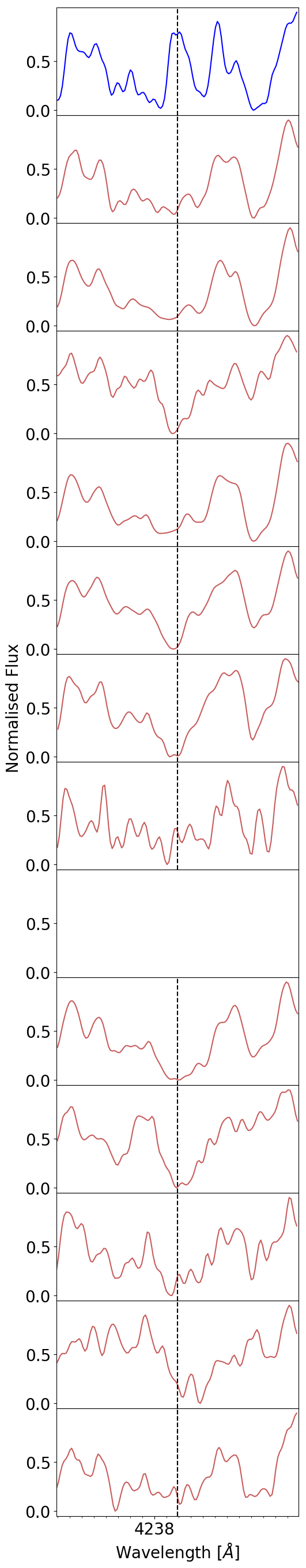
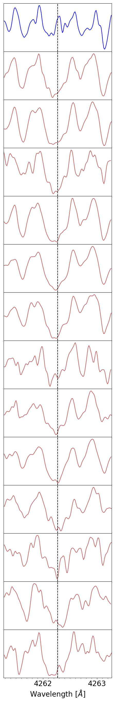
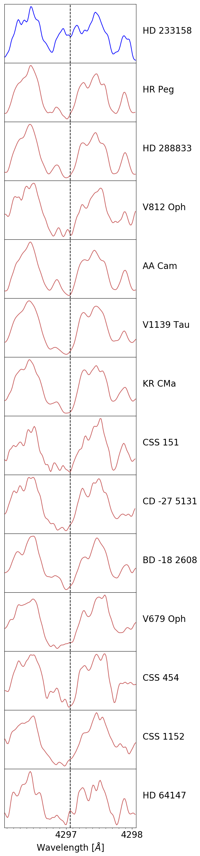
Figure 1: The spectral region around the three (4238.19, 4262.27 and 4297.06 Å) Tc I lines in our sample of Tc-rich S stars. For comparison purposes, the spectrum of a Tc-poor S star (HD 233158, in blue in the top panels) from S18 is also plotted. The spectra have been arbitrarily normalized and binned by a factor of 1.5 to increase the S/N ratio. The Tc I line at 4238.19 Å could not be used for CD -27^∘5131 as local normalization was hampered by a nearby cosmic ray hit.

4 Derivation of the atmospheric parameters

Disentangling the intricate parameter space of S stars has always been a challenging task because their spectra are dominated by molecules. The atmospheres of S stars are complex as the thermal structure is dependent on their chemical composition (C/O and, to a lesser extent, heavy elements). Different methods have been used in the past for the stellar parameters determination. For instance, in their pioneering work, Smith & Lambert (1985) derived $T_{\mathrm{eff}}$ from the $(V-K)$ colors and $\log g$ from the standard $\log g$ - mass relationship where they estimated the masses by comparing the positions of the S stars in the HR diagram with the evolutionary tracks. However, the $T_{\mathrm{eff}}$ - $(V-K)$ relation valid for M-type giants has been shown to be inappropriate for S-type stars (SVE17) because of the spectral energy distribution (SED) alteration (mainly by ZrO, LaO and YO bands) induced by the non-standard chemical composition of S stars. New MARCS model atmospheres (Gustafsson et al., 2008) were designed to cover the full parameter range of S stars, with $T_{\mathrm{eff}}$ from 2700 K to 4000 K, $\log g$ from 0 to 5, [Fe/H] of 0.0 and -0.5, C/O values of 0.500, 0.752, 0.899, 0.925, 0.951, 0.971, 0.991 and [s/Fe] of 0.0, 1.0 and 2.0 (SVE17).

In the current study, the stellar parameters are determined as in S18. In summary, the high-resolution HERMES spectra are compared with a grid of $\sim 3500$ synthetic spectra computed from the S star MARCS models to obtain atmospheric parameter estimates $T_{\mathrm{eff}}$, log $g$ and [Fe/H]. The fitting is undertaken over small spectral windows (listed in Appendix Table 14) because HERMES spectra cannot be considered as flux-calibrated over their whole wavelength range. The fit with the lowest total $\chi^{2}$ value then identifies the best-fitting model, providing a first estimate of the atmospheric parameters.

The stellar luminosities were calculated using the distances derived from the Gaia EDR3 parallaxes after applying the zero-point correction from Lindegren et al. (2020), the reddening $E_{B-V}$ computed from Gontcharov (2017) and the bolometric correction in the $K$ band as computed from the MARCS model atmospheres. Combining the $T_{\mathrm{eff}}$, metallicity and luminosity, we located the stars in the HR diagram and compared them with STAREVOL (Siess, 2006) evolutionary tracks to estimate their current stellar masses.

A new surface gravity was then computed and the procedure iterated (as described in Fig. 5 of S18) until the $\log g$  retrieved from spectral fitting was consistent with the one obtained from the HR diagram. The uncertainties on the stellar parameters were obtained from the variations of the atmospheric parameters while iterating for $\log g$. Our final set of parameters and the corresponding uncertainties are presented in Table 3. A further discussion of the reliability of the stellar masses thus found, based on their correlation with the height above the galactic plane and with 2MASS photometry, may be found in Appendix A.

Table 3: Atmospheric parameters for S stars.

Name	$T_{\rm eff}$	$L$	$\log g$	[Fe/H]	$\sigma_{\rm[Fe/H]}$	C/O	[s/Fe]	Mcurr	Mini
	(K)	($L_{\odot}$)	(dex)				(dex)	($M_{\odot}$)	($M_{\odot}$)
V1139 Tau	3400	6600	1	-0.06 (13)	0.13	0.752	1	3.3	3.5
	(3400 - 3500)	(6200 - 6900)	(1 - 3)			(0.500 - 0.752)	(1 - 1)
CSS 151	3500	4600	1	-0.25 (14)	0.14	0.500	1	2.6	3.2
	(3500 - 3600)	(4100 - 5200)	(1 - 3)			(0.500 - 0.899)	(1 - 1)
HD 288833	3600	1700	1	-0.30 (13)	0.14	0.500	0	1.3	1.4
	(3600 - 3600)	(1600 - 1800)	(1 - 2)			(0.500 - 0.752)	(0 - 1)
KR CMa	3400	4800	1	-0.01 (13)	0.22	0.500	1	2.8	3.0
	(3400 - 3500)	(4600 - 5000)	(1 - 3)			(0.500 - 0.752)	(1 - 1)
AA Cam	3600	3700	1	-0.32 (15)	0.13	0.500	0	2.4	2.5
	(3600 - 3600)	(3600 - 3900)	(1 - 2)			(0.500 - 0.899)	(0 - 1)
HD 64147	3500	5400	0	-0.67 (11)	0.10	0.500	0	2.7	2.9
	(3500 - 3600)	(4900 - 5900)	(0 - 1)			(0.500 - 0.752)	(0 - 1)
CSS 454	3500	2900	1	-0.38 (12)	0.14	0.500	1	1.8	1.9
	(3500 - 3600)	(2600 - 3400)	(1 - 3)			(0.500 - 0.899)	(1 - 1)
CD -27∘5131	3400	9200	0	-0.30 (9)	0.12	0.500	1	3.4	3.7
	(3400 - 3600))	(8300 - 10100)	(0 - 3)			(0.500 - 0.899)	(1 - 1)
BD -18∘2608	3500	2400	1	-0.31 (13)	0.16	0.752	1	1.5	1.6
	(3500 - 3600)	(2300 - 2600)	(1 - 3)			(0.500 - 0.899)	(1 - 1)
V812 Oph	3500	3000	1	-0.37 (13)	0.13	0.500	1	1.8	2.0
	(3500 - 3500)	(2700 - 3200)	(1 - 2)			(0.500 - 0.899)	(1 - 1)
V679 Oph	3600	4600	1	-0.52 (9)	0.14	0.899	1	2.0	2.1
	(3600 - 3600)	(4300 - 4800)	(1 - 1)			(0.752 - 0.899)	(1 - 2)
CSS 1152	3400	4400	1	-0.14 (6)	0.13	0.971	1	2.8	3.0
	(3400 - 3600)	(4100 - 4700)	(1 - 2)			(0.899 - 0.971)	(1 - 2)
HR Peg	3500	4900	0	-0.34 (13)	0.17	0.500	0	2.2	2.3
	(3500 - 3600)	(4500 - 5200)	(0 - 4)			(0.500 - 0.752)	(0 - 1)

5 Chemical abundance determination

The abundance determination methodology is the same as the one adopted in S18 and S19. We compared the observed spectra with synthetic spectra generated using Turbospectrum v15.1 (Plez, 2012) and MARCS model atmospheres of S stars with the parameters derived in Sect. 4. We have made use of the same input molecular line lists as in SVE17, atomic line list as in the Gaia-ESO survey (Heiter et al., 2020) and varied the abundances till a satisfactory agreement could be found.

5.1 Li

We used the Li i line at 6707.8 Å to derive the Li abundance. This line is known to be blended with a neighboring Ce ii line at 6708.099 Å in the warmer post-AGB stars (Reyniers et al., 2002). However, we did not identify any dominating blend from this line to the Li i line in our sample stars. In Fig. 2 we present examples of stars with a good (bottom panel) as well as bad (top panel) spectral-synthesis fit of the considered Li line. We could derive the Li abundance for only three stars from our sample, namely HR Peg, V679 Oph and Vy 12. For these stars, the absorption features of the Li doublet located at 6707.8 Å are very clear. For the rest of the sample, there were severe blends in the Li line (top panel of Fig. 2), so only upper limits on the Li abundances could be derived. The results are listed in Table  7.

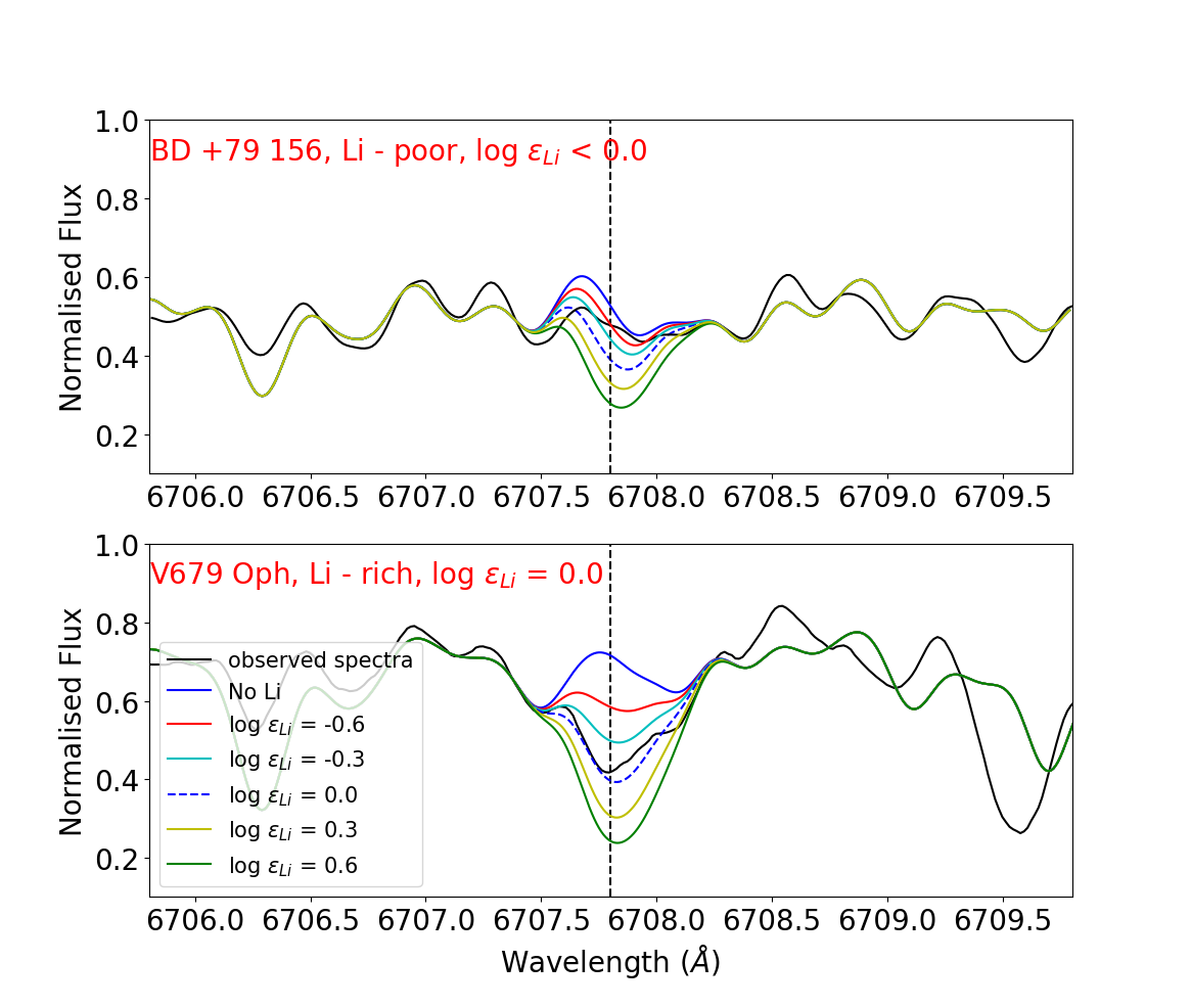
Figure 2: Illustration of the fit quality between the observed and synthetic spectra of BD +79^∘156 (top panel) and V679 Oph (bottom panel) around the Li line at 6707.8 Å.

The Li abundances of all the intrinsic S stars of our sample are generally low except for HR Peg. HR Peg was found to be a Li-rich star also by Vanture et al. (2007) who classified the star as a high-mass star ($M>3$ M_⊙) with hot bottom burning (HBB) as an explanation for the Li abundance. However, our mass estimate for HR Peg is $M_{\mathrm{curr}}$ = 2.2 M_⊙, in agreement with the 2.0 M_⊙ value found by Neyskens et al. (2015). Therefore, HR Peg does not appear to be massive enough to be producing Li through HBB. Other plausible explanations involve some extra mixing in low-mass AGB stars (e.g. Charbonnel & Balachandran, 2000; Uttenthaler et al., 2007; Uttenthaler & Lebzelter, 2010) or the engulfment of planets/brown dwarfs (Siess & Livio, 1999).

5.2 C, N, O

We used the CH bands around 4250 Å to determine the C abundance. The sensitivity of these bands to the carbon abundance is limited in S-star spectra because CH bands are blended with mainly TiO and ZrO (as can be seen from Fig. 16 of SVE17). It was not possible to derive the O abundance because the $\lambda$ 6300.3 Å  O i line lies in a severely blended region. We used the solar oxygen abundance (Asplund et al., 2009) scaled with respect to the metallicity and included an alpha enhancement ([$\alpha$/Fe] = $-0.4\;\times$ [Fe/H]) for [Fe/H] $\geq-0.5$. The uncertainty on C/O was estimated from the range of values of the C/O providing an acceptable fit to the CH G-band.

The N abundance was then determined from the CN lines available in the region 8000-8100 Å. The line list for these CN lines was taken from Sneden et al. (2014).

5.3 [Fe/H]

We used the same line lists as S18 and S19 (see also Appendix Table 15) for Fe line synthesis. Between 9 and 15 Fe lines were used to derive the metallicity for all the sample stars, except for the star Vy 12, for which only six Fe lines could be used, as the other lines were strongly blended by molecules because of the high C/O of this object (0.97). The derived metallicity as well as the standard deviation due to line-to-line scatter are listed in Table 3.

5.4 Light s-process elements (Sr, Y, Zr, Nb)

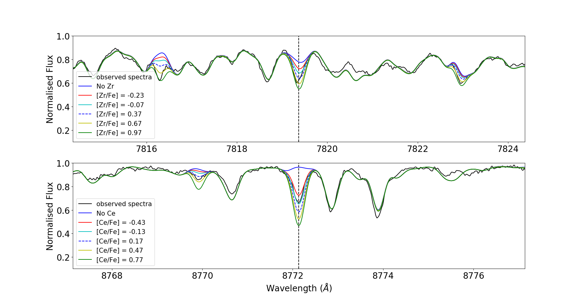
Figure 3: Illustration of the fit between the observed and synthetic spectra for the S star HR Peg. The top panel presents 5 Å around the Zr I line at 7819.37 Å and the bottom panel around the Ce II line at 8772.135 Å.

The line list of S18 was used and complemented as documented in Appendix Table 15. The strontium abundance could be derived only for HD 288833, BD-18^∘2608, and V679 Oph. The Y abundance was measured for all the sample stars. The Zr abundance was measured for all stars except KR CMa using the two Zr i lines at 7819.37 and 7849.37 Å with transition probabilities from laboratory measurements (Biémont et al., 1981). Some Nb i lines from Appendix Table 15 could not be used in some stars. In fact, none of the Nb i lines could be used for CSS 151 because of the low S/N of its spectrum. The Nb abundance could therefore not be derived for this star.

5.5 Heavy s-process elements (Ba, Ce, Nd)

We derived the barium abundance using only one Ba i line located at 7488.07 Å. The cerium abundance was determined using the Ce ii lines from S18 together with some new lines located at 7580.91, 8025.57, 8394.51, 8405.25, and 8769.91 Å. There is a huge scatter in the Ce abundances for HR Peg, $o^{1}$ Ori, KR CMa, BD+79^∘156, and HD 64147 despite the use of Ce ii lines displaying satisfactory fits. The bottom panel of Fig. 3 illustrates the fact that even neighboring Ce ii lines (at 8769.91 and 8772.13 Å) can provide discrepant abundances (by $\sim$ 0.4 dex in this case). As explained in Karinkuzhi et al. (2018), cerium abundances derived using only Ce ii lines above 7000 Å are $\sim$ 0.3 dex lower than the ones derived from Ce ii lines in the range 4300-6500 Å. These authors mention that this difference might be imputable to non-LTE (non-local thermodynamic equilibrium) effects. This could be the reason for the sub-solar cerium abundances in some of our stars, as they were determined using only red Ce ii lines ($\lambda>7000$ Å). These uncertain abundances are marked with a colon in Tables 8 and 9.

5.6 Other heavy elements (Pr, Sm, Eu)

Good Eu ii and Pr ii lines are located in the bluer part of the spectrum and could be used in some stars where the blending was weak. The Sm abundance was derived when possible using the Sm ii 7042.20 and 7051.55 Å lines. These lines are well fitted and yield consistent abundances.

5.7 Tc

All three Tc i resonance lines at 4238.19, 4262.27 and 4297.06 Å are heavily blended (Little-Marenin & Little, 1979). We first derived the other s-process abundances in order to reproduce these blends as precisely as possible. The 4262.27 Å line is the best reproduced by our spectral synthesis. Its blends, consisting in two neighbouring lines of Nb i (at 4262.050 Å) and Gd ii (at 4262.087 Å) were identified in Van Eck & Jorissen (1999). The Tc abundance was derived from the 4262.27 Å Tc i line in our sample stars as well as in all intrinsic S stars from S18 and S19 (Table 7).

5.8 Uncertainties on the abundances

The uncertainties on the abundances have been computed using the ones of the S star V915 Aql investigated in S18. The atmospheric parameters of V915 Aql are representative of those of most of our sample stars, hence we computed the elemental abundance error by quadratically adding the elemental standard deviation due to line-to-line scatter, the abundance errors due to parameter uncertainties of V915 Aql as derived in S18 (see also Appendix B), and a term of 0.1 dex to take into account continuum placement errors. For abundances that were derived using only one line, an arbitrary line-to-line scatter of 0.1 dex was assumed. Error bars on Tc abundances were estimated as the range of Tc abundances providing an acceptable fit of the Tc i 4262.27 Å line. The final elemental uncertainties on abundances are listed in Appendix Tables 8, 9, and 10.

6 HR diagram of S stars

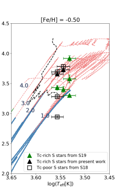
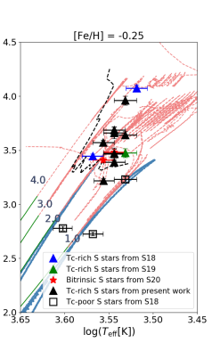
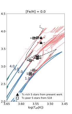
Figure 4: HR diagram of intrinsic (filled triangles) S stars from our large sample and extrinsic (open squares) S stars from S18 along with the STAREVOL evolutionary tracks corresponding to the closest metallicities. The red giant branch is represented in blue, the core He-burning phase in green, whereas the red dashed lines correspond to the AGB tracks. The black dashed line represents the predicted onset of the third dredge-up, i.e., the lowest stellar luminosity following the first occurrence of a TDU episode (down to 1.5, 1.3, 1.0 M_⊙ for [Fe/H] = 0.0, -0.25, -0.50 respectively).

In Fig. 4 we present an HR diagram collecting Tc-rich S stars studied in S18, S19, and S20 as well as those of the present work, together with Tc-poor stars from S18. We used the final stellar parameters presented in Table 2. The errors on $T_{\mathrm{eff}}$ are taken from Table 2. For HD 288833, V812 Oph, AA Cam, and V679 Oph for which $T_{\mathrm{eff}}$ did not change during the $\log g$ iterations, we imposed a standard symmetric error of 100 K on their $T_{\mathrm{eff}}$. The asymmetric error on the luminosity was derived after propagating the error on the parallax. The evolutionary tracks displayed in Fig. 4 were computed with the STAREVOL code (Siess et al., 2000) and are described in detail in Escorza et al. (2017). Briefly, we use standard input physics with a mixing-length parameter $\alpha=1.75$, grey surface boundary conditions and the Asplund et al. (2009) solar mixture. Opacity enhancement due to the formation of molecules in carbon-rich atmospheres is also accounted for following the formulation of Marigo (2002). The Schröder & Cuntz (2007) mass-loss prescription is activated up to the end of core helium burning followed by the Vassiliadis & Wood (1993) formulation during the AGB phase. We also consider overshooting below the convective envelope following the exponential decay expression of Herwig et al. (1997) with the parameter $f_{\mathrm{over}}=0.01$. Models were computed for various metallicities, including [Fe/H] = 0, -0.25 and -0.5.

There is a clear segregation between the location of intrinsic and extrinsic S stars in the HR diagram. Indeed, whatever the considered metallicity range, intrinsic S stars are always located above the black dotted line (see Fig. 4) marking the predicted onset of TDU for masses above 1.5 M_⊙. Whereas it is obvious that Tc-rich stars must be TP-AGB stars (because of the Tc detection), such a consistency between the luminosity of the third dredge-up onset in theoretical models, and the luminosity of observed intrinsic S stars, which are the least evolved objects identified as TP-AGB stars, was not as clearly demonstrated so far.

Table 4 summarizes the observational constraints on the TDU first occurrence in terms of luminosity, initial mass and metallicity. For each mass and metallicity bins, we indicate the lowest luminosity of intrinsic S stars from our so-called large sample collecting stars from S18, S19, S20 and from the current work. These luminosities represent an observational upper limit on the TDU first occurrence in AGB stars, in the sense that Tc-rich stars are observed at such luminosities, so that TDU must have already occurred by the time the star reaches this position in the HR diagram. However, since S stars are the first objects on the AGB to show clear signatures of TDU events (Tc and ZrO), this upper limit must be quite close to the genuine TDU occurrence line. It can be used as an observational constraint to be satisfied by the stellar evolutionary models of the corresponding masses and metallicities.

Table 4: Observed lowest luminosities of intrinsic S stars in different mass and metallicity bins (collected from this work, S18, S19 and S20).

	Stars	Initial mass (M⊙)	[Fe/H]	$L_{\rm TDU}$ ($L_{\odot}$)
Mini ¡ 1.0 M⊙	V915 Aql	1.0	-0.5	2000
1.0 M⊙¡ Mini ¡ 1.5 M⊙	IRAS 06000+1023 (CSS 182)	1.3	-0.40	2500
	HD 288833	1.4	-0.30	1700
1.5 M⊙¡ Mini ¡ 2.0 M⊙	BD -18 2608	1.6	-0.31	2400
	V812 Oph	2.0	-0.37	3000
2.0 M⊙¡ Mini ¡ 2.5 M⊙	BD+79∘156	2.1	-0.16	2600
	V679 Oph	2.1	-0.52	4600
2.5 M⊙¡ Mini ¡ 3.0 M⊙	HD 64147	2.9	-0.67	5400
	CSS 1152	3.0	-0.14	4400
	KR CMa	3.0	-0.01	4800
Mini ¿ 3.0 M⊙	CSS 151	3.2	-0.25	4600
	V1139 Tau	3.5	-0.06	6600

7 Discussion on the abundances and comparison with STAREVOL nucleosynthesis predictions

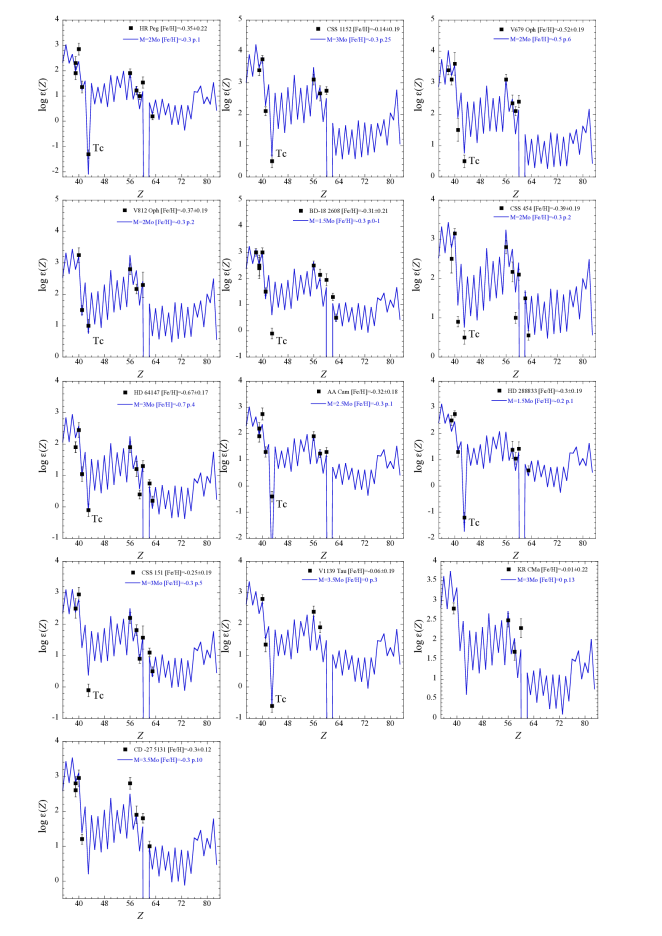
Figure 5: Measured s-process element abundances compared with the nucleosynthesis predictions. The blue line represents the nucleosynthesis predictions compatible with the mass and metallicity of the individual stars. The number of pulses $n$ required to best-match the measured abundances is mentioned in the label of every panel as ”p.$n$”.

The elemental abundances derived following the methodology presented in Sect. 5 allow us to investigate nucleosynthesis in intrinsic S stars. We compare the measured abundance profiles of our sample stars with the nucleosynthesis calculations of the STAREVOL code (Goriely & Siess, 2018) which uses an extended network of 411 species.

The predicted and measured abundance distributions are presented in Fig. 5. The pulse number is chosen in order to optimally match both the overabundance level and the location in the HR diagram. We find a good overall agreement between the predicted and measured distributions of heavy elements. In particular, the peak of heavy s-elements is well reproduced in all stars. However, problems persist with the light elements such as carbon or oxygen, as discussed in Sect. 7.1, and with some heavy elements, e.g. Ce as discussed in Sect. 5.4. The models do account for most of the derived Tc abundances; however, we note that abundance predictions for Tc are extremely sensitive to the pulse number and to the amount of dilution in the stellar envelope due to the initial absence of Tc in the star. Hence, the agreement between predicted and measured abundances may be poor in some cases, for e.g., CSS 151, BD -18^∘2608, and CSS 454. We now investigate specific element ratios.

7.1 [C/Fe] and [s/Fe]

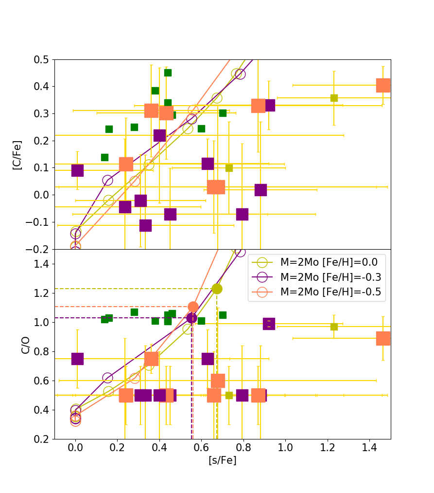
Figure 6: Top panel: measured [C/Fe] abundances as a function of [s/Fe] for our large sample of Tc-rich S stars (light green, purple and orange squares) where the size of the symbol increases with decreasing metallicity, considering 3 metallicity bins: [Fe/H] in [0.0;$-0.2$]: light green, [$-0.2$; $-0.4$]: purple, below $-0.4$: orange. Tc-rich carbon stars from Abia et al. (2002) are shown as green squares. Bottom panel: derived C/O ratio versus [s/Fe] for the same stars. Predictions for a 2 M_⊙  STAREVOL model at metallicity [Fe/H] = 0.0 (light green), $-0.3$ (violet) and $-0.5$ (orange) are overplotted. The empty circles along the tracks indicate the successive TDUs, while the three filled circles mark the first TDU allowing to reach C/O$>1$ in each model.

The surface composition of TP-AGB stars should reflect the addition of ¹²C originating from the He-burning shell and s-process material produced either radiatively in the interpulse or in the convective thermal pulses for more massive objects. The TDU is then responsible for transporting these products to the stellar surface. As the star evolves on the TP-AGB, its carbon abundance should thus increase along with its s-process over-abundances. Eventually the star becomes carbon-rich when the C/O ratio exceeds unity. However, massive AGB stars with M${}_{\mathrm{ini}}\ga 4$ M_⊙  experience HBB and can efficiently burn the dredged-up carbon to produce mainly ¹⁴N. In the top panel of Fig. 6 we present the carbon abundance as a function of s-process abundance for our intrinsic S star sample. The [s/Fe] index has been calculated using the Y, Zr and Ba abundances and is listed in Table 11. In order to compare this trend with that of the stars from the next evolutionary stage, we added in Fig. 6 the Tc-rich carbon stars from Abia et al. (2002). A larger marker size indicates a lower metallicity (stars are grouped in three [Fe/H] bins: [$-\infty,-0.4$], [$-0.4,-0.2$], and [$-0.2,0$]).

In the top panel of Fig. 6, the trend of increasing [C/Fe] with increasing [s/Fe], expected for TP-AGB stars, is not marked. Nevertheless, the S stars most enriched in s-process elements are the ones with the highest carbon abundance. The carbon stars have higher carbon abundances than most S stars but are characterized by [s/Fe] indices in the same range as those of the bulk of S stars. A group of intrinsic S stars have similar [s/Fe] and [C/Fe] ratios as carbon stars. This can be explained as follows: the carbon stars from Abia et al. (2002) have solar metallicities while the intrinsic S stars belonging to the group with similar [C/Fe] (in the range 0.2 to 0.35 dex) have lower metallicities (in the range -0.2 to -0.5 dex). Because [$\alpha$/Fe] increases with decreasing metallicity in the range $-0.5<$[Fe/H]$<0$, this group of S stars has a higher initial [O/Fe] compared to carbon stars, enabling their O-rich classification.

The [C/Fe] abundances in this work were derived from the C/O ratios assuming solar oxygen abundance scaled with respect to metallicity and taking into account an $\alpha$-element enhancement (Sect. 5.2). The determination of [C/Fe] is therefore quite indirect. We thus present in the bottom panel of Fig. 6 the C/O ratios. Their determination is very robust, given the high sensitivity of molecular bands to the C/O ratio. As expected, there is no overlap between C/O ratio of C stars and S-type stars. We note that 3 S-type stars have C/O ratios close to, but definitely lower than 1: indeed their C/O of 0.899, 0.971, and 0.998, produces an observed spectrum markedly different from the spectrum of an SC star (characterized by C/O $=1$).

A common misunderstanding is that S stars have C/O $=1$. This statement is often encountered in the literature even as a definition of S-type stars. Once again (see also Van Eck et al., 2017), we stress here that only S stars with the highest [s/Fe] values have C/O ratios approaching (but not reaching) unity. Most S-type stars have intermediate C/O ratios (between 0.5 and 0.8). Stars with C/O $=1$ are actually classified as SC or CS stars.

Figure 6 also compares the measured carbon and s-process abundances with the nucleosynthesis predictions at three different metallicities ([Fe/H] = 0.0, -0.3 and -0.5). The filled circles along the tracks mark the thermal pulses turning the C/O ratio to values above 1, thus changing the (model) stars into carbon stars. First, the different models predict a tight correlation between C/O and [s/Fe], whereas there is a large scatter in measured [s/Fe] at a given C/O. Second, theoretical calculations show a much faster increase of C/O with [s/Fe] than what is actually measured in stars. For example, all models predict that stars with [s/Fe] $\geq 0.55$ should have C/O $>1$ (and be carbon stars), whereas many S stars (which must have C/O $<1$) are observed with such large s-process enrichments. In other words, in theory, high s-process enrichments go along with very high C/O ratios which are incompatible with S-star classification. The reason why carbon stars do not show such large s-process overabundances (stronger line blending? dust obscuration of the most evolved objects?) is yet unclear.

Finally, we remark that Fig. 6 reveals the existence of one S star, $o^{1}$ Ori, with very mild – if any – enrichment in s-process elements (see [s/Fe] in Table 11, Figure 4 and Table A.1 from S20 for individual heavy-element abundances). This star is another example of the ”Stephenson M-type stars” uncovered by Smith & Lambert (1990). Nevertheless, it shows clear Tc signatures (Figure 1 of S20). The possible reasons for the low [s/Fe] index of $o^{1}$ Ori are discussed in detail in S20 and Jorissen et al. (2019).

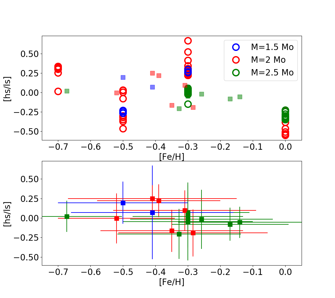
Figure 7: The distribution of [hs/ls] as a function of metallicity for the intrinsic S stars of our study (filled squares). The hs-index has been calculated using Ba and Nd, and the ls-index using Y and Zr. The symbols are color-coded with respect to the initial mass in the bins M_ini ¡ 1.5 M_⊙  (blue), 1.5 $\leq$ M_ini ¡ 2.5 M_⊙ (red), and M_ini $\geq$ 2.5 M_⊙ (green). Note that these mass bins are designed to match the [hs/ls] STAREVOL predictions only available for M_ini = 1.5, 2, 2.5 M_⊙. Open circles denote the predictions from pulse to pulse for the different initial masses.

7.2 [hs/ls] and metallicity

We now investigate the potential correlations between the heavy (hs) to light (ls) s-process element ratio [hs/ls], mass and metallicity. The neutron irradiation index [hs/ls] is actually expected to increase with decreasing metallicity (Goriely & Mowlavi, 2000), as the number of neutrons per iron seed increases.

From our measured abundances we find a large scatter in [hs/ls] with respect to metallicity (Fig. 7), within our limited range of metallicity.  De Smedt et al. (2015, 2016) also reported such a scatter in the [hs/ls] – [Fe/H] plane from their study of s-process enriched post-AGB stars. However, the evolutionary link between post-AGB stars and intrinsic stars remains to be firmly established. Figure 7 also shows the absence of a clear correlation between the [hs/ls] ratio and the initial stellar masses.

When compared with the theoretical predictions accounting for the pulse-to-pulse variation, plotted in the top panel of Fig. 7, we find that the overall range covered by our measured [hs/ls] indices is compatible with that of the predicted abundances of the theoretical models. However, the [hs/ls] model predictions are not available for the complete metallicity range covered by our measured [Fe/H].

7.3 Technetium abundances

7.3.1 [s/Fe], C/O and Tc

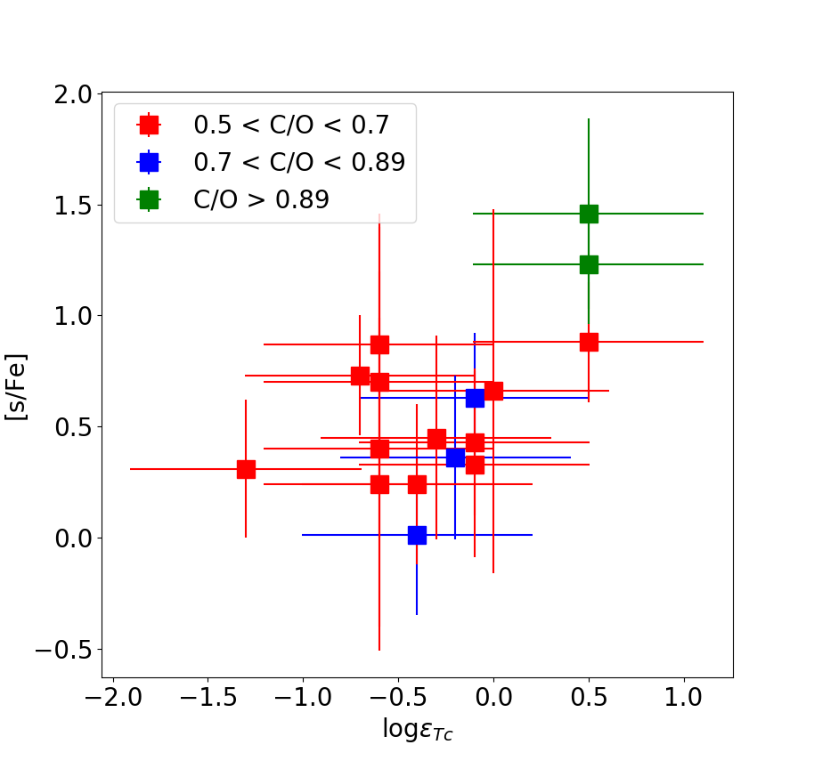
Figure 8: [s/Fe] index versus Tc abundance. The different colors represent different C/O ratio bins as described in the figure.

Figure 8 presents [s/Fe] (calculated as described in Sect. 7.1 using Y, Zr and Ba abundances) as a function of the Tc abundance, for different C/O ratio bins. The stars with the highest [s/Fe] and Tc abundances are also the ones with the highest C/O ratios, which is consistent with expectations from TP-AGB evolution. However, it is worth mentioning that whereas [s/Fe] is predicted to monotonically increase as the star ascends its AGB (see Fig. 6, this is also true for C/O if there is no HBB, and for luminosity, set aside the luminosity variations during thermal pulses), the technetium abundance has a more complex behaviour, because the ⁹⁹Tc half life (210 000 yrs) is not totally negligible with respect to the TP-AGB duration. For example, the evolution of the technetium-to-zirconium abundance ratio is not flat but shows a non-trivial evolution displayed in Fig. 2 of Neyskens et al. (2015). The lack of a clear trend in Fig. 8 is therefore not surprising.

7.3.2 Luminosity and Tc

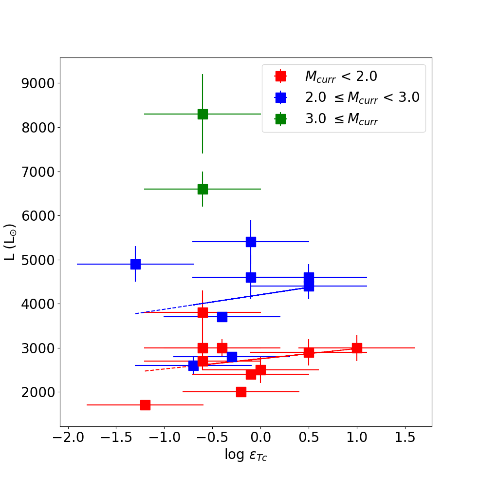
Figure 9: Stellar luminosity as a function of Tc abundance. The symbols are color coded according to their mass bin. The blue and red dashed lines represent the linear least-squares fit for the stars in the corresponding mass bin.

In Fig. 9 we compare the Tc abundances and the luminosities of the sample stars. A large scatter in luminosity is present for each Tc abundance. If we focus on a specific mass bin, there is a loose trend of increasing Tc abundance with increasing luminosity, represented by the dashed least-square fit lines in Fig. 9. We also find that the most luminous and massive star in Fig. 9 has a relatively moderate Tc overabundance. A likely explanation is the larger dilution of s-elements in the bigger envelope of more massive AGB stars. Besides, with increasing stellar mass, the mass of the ¹³C pocket responsible for the s-process, as well as that of the thermal pulses, are reduced because of the stronger compression of the shells induced by the larger core mass. Lower surface abundances of s-process elements are thus expected in higher-mass TP-AGB stars (García-Hernández et al., 2013).

7.4 The Zr-Nb plane and intrinsic/extrinsic stars segregation

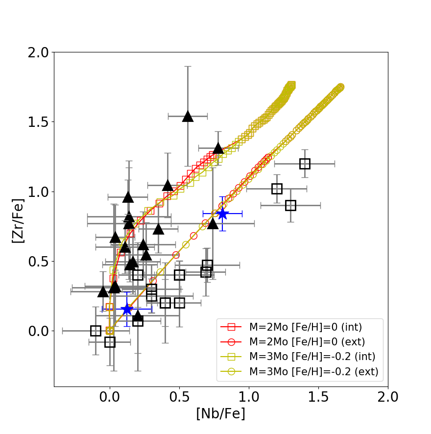
Figure 10: [Zr/Fe] as a function of [Nb/Fe] for the intrinsic S stars (black filled triangles) and extrinsic S stars (open squares) from S18 compared with the nucleosynthesis predictions for different initial masses and metallicities. The bitrinsic S stars from S20 are plotted with a blue star symbol. The ”ext” and ”int” labels next to the model parameters refer to extrinsic (respectively intrinsic) model abundances.

A particular attention can also be paid to the Zr and Nb abundances that can be used as extrinsic/intrinsic star markers (Neyskens et al., 2015). As already mentioned in Sect. 1, niobium is mono-isotopic and can only be produced by the decay of  ⁹³Zr (with a half-life of $1.53\times 10^{6}$ yr). Intrinsic S stars are freshly producing s-process elements including ⁹³Zr, and there is not enough time on the TP-AGB for a significant production of ⁹³Nb. On the contrary, in extrinsic S stars, enough time has elapsed since the end of the nucleosynthesis in the companion for ⁹³Zr to have totally decayed into ⁹³Nb. As expected, intrinsic and extrinsic S stars follow different trends in the [Zr/Fe] – [Nb/Fe] plane, where intrinsic S stars have [Zr/Nb] ¡ 1 while extrinsic stars have [Zr/Nb] $\sim$ 1 (Neyskens et al., 2015, S18). The Zr – Nb plane has been studied extensively for extrinsically-enriched objects: the high Nb abundance in extrinsic stars has been demonstrated in various extrinsic-star families among which CH and CEMP stars (Karinkuzhi et al., 2018, 2021). The apparent shift of extrinsic stars from the STAREVOL 2 – 3 M_⊙  predictions by a few tenths of a dex is as well discussed in Karinkuzhi et al. (2018). These authors speculated that this shift could arise due to the oscillator strengths of the two Zr lines used to derive the Zr abundance of the extrinsic S stars, which have a tendency to yield abundances that are about 0.1 dex too low in the benchmark stars of their sample (Arcturus and V762 Cas). Here we populate the high-Zr, low-Nb region of this plane, adding constraints from the Tc-rich S stars.

Figure 10 confirms, on the basis of our so-called large sample of intrinsic S stars, the nice segregation between extrinsic and intrinsic stars in the [Zr/Fe] – [Nb/Fe] plane (with one exception discussed below). We also compare the measured Zr and Nb abundances with nucleosynthesis predictions from STAREVOL for intrinsic and extrinsic stars of 2 and 3 M_⊙, and metallicities [Fe/H] = 0.0 and -0.2. In Fig. 10, the intrinsic S stars from our sample have [Zr/Fe] ¡ 1.6 and follow the trend predicted for TP-AGB stars (open squares in red and green). It is worth mentioning that some ⁹³Zr decay (inducing some ⁹³Nb production) is both predicted and observed, as can be seen from the fact that highly-enriched (high-Zr) intrinsic stars, which are the most evolved S stars on the TP-AGB, tend to have the largest Nb enrichments, and nicely follow the STAREVOL inclined trend in the [Zr/Fe] – [Nb/Fe] plane.

The two Tc-rich S stars $o^{1}$ Ori and BD+79^∘156 are ’bitrinsic’ S stars as they are Tc-rich (intrinsic) but show signs of binarity together with a large Nb enrichment (for the corresponding [Zr/Fe] ratio), two evidences that they are also extrinsic stars, as discussed in S20. In addition to these two stars, the use of Gaia EDR3 parallaxes revealed a potentially new ‘bitrinsic’ candidate, BD $+34^{\circ}$1698. We re-computed the s-process abundances of this star as its stellar parameters (mainly mass and $\log g$) changed when Gaia DR2 parallaxes were replaced by Gaia EDR3. The revised s-process abundances of BD$+34^{\circ}$1698 are presented in Appendix Table 13. It has a [Zr/Nb] ratio close to unity, along with clear signatures of Tc (see Fig. C1 of S19), hence it qualifies as a ‘bitrinsic’ candidate. Wang & Chen (2002) classified it as a candidate extrinsic S star based on its IRAS photometry. Two spectra taken with the Hermes spectrograph revealed a clear radial-velocity variation: $V_{r}=18.59\pm 0.05$ km s^-1 on JD $2\,457\,502.44$ and $V_{r}=22.59\pm 0.09$ km s^-1 on JD $2\,459\,289.51$. Our detection of the binary motion associated to a clear Tc enrichment and a [Zr/Nb] ratio close to unity unambiguously classify BD $+34^{\circ}$1698 as a member of the restricted family of bitrinsic stars (S20). Lastly, Fig. 10 confirms that the Zr-Nb analysis successfully serves as an additional test (apart from Tc) for the classification of S stars as intrinsic or extrinsic.

8 Conclusions

Thanks to the combination of Gaia EDR3 parallaxes and the high-resolution HERMES spectra, we have determined the stellar parameters of a sample of 13 intrinsic S stars with metallicities in the range -0.7 ¡ [Fe/H] ¡ 0. We then derived their s-process element abundances. The heavy-element abundances of intrinsic S stars reveal their rich nucleosynthetic history. The main results from our study can be summarized as follows:
(i) The Gaia EDR3 HR diagram of S stars confirms that intrinsic S stars are more evolved than their extrinsic counterparts.
(ii) The luminosity lower limits for the occurrence of TDU in different mass and metallicity ranges provided in Table 4 can be used to constrain AGB evolutionary models.
(iii) The objects from our sample with the largest C/O ratios are also the ones with the largest [s/Fe], which is consistent with TP-AGB evolution predictions.
(iv) However, we clearly demonstrate the too rapid increase of the C/O ratio with respect to [s/Fe] in model predictions.
(v) The measured s-process abundances of intrinsic S stars are in good agreement with the AGB nucleosynthesis predictions for models of the corresponding mass and metallicity. In particular, the Zr and Nb abundances are matching very well the predicted trend for intrinsic S stars, confirming our previous finding (S18, S20) that the Nb abundance can be used as an intrinsic/extrinsic diagnostic as efficient as the Tc presence/absence.
(vi) We present Tc abundances for a large sample of intrinsic S stars (20 stars). We find that the stars with the highest C/O ratios tend to be the ones with the highest Tc abundances.

In conclusion, the current investigation of a sample of intrinsic S stars has extended our understanding of their properties, in particular their location in the HR diagram and their chemical characterization considering $\sim$ 10 chemical elements, including C/O ratio and the radioactive element technetium.

Appendix A Reliability of the S-star masses

A.1 Height above the galactic plane

.

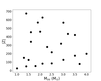
Figure 11: Height above the galactic plane for the sample intrinsic stars and for the intrinsic stars from S18, S19 and S20, as a function of their initial mass (left panel) or luminosity (right panel).

Figure 11 presents the height above the galactic plane ($|Z|$) of our sample stars. Though a large $Z$ scatter is present at low masses, the maximum $|Z|$ value decreases with increasing mass, as expected. This trend somehow validates the masses estimated in the present paper. Nevertheless, the limited size of the present sample, and the absence of bias control in this sample, precludes us from drawing any further conclusion.

A.2 Gaia-2MASS photometry

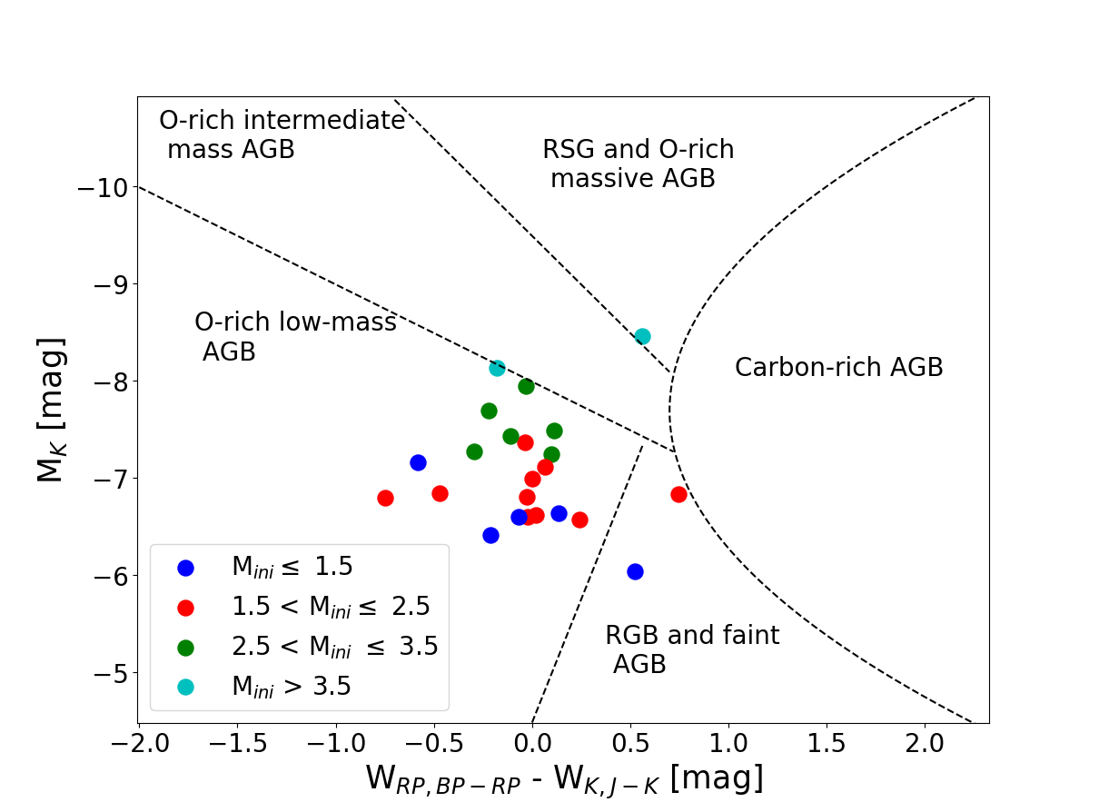
Figure 12: The $W_{RP,BP-RP}-W_{K,J-K}$ vs $M_{K}$ diagram of our sample of Tc-rich S stars. The definitions of the boundaries (black dashed lines) are from Lebzelter et al. (2018).

Lebzelter et al. (2018) present a classification of AGB stars using Gaia and 2MASS photometry, in the plane $W_{RP,BP-RP}-W_{K,J-K}$ vs $M_{K}$, where $M_{K}$ is the absolute $K_{S}$ magnitude from 2MASS and Gaia EDR3 parallaxes. The Wesenheit functions $W_{RP,BP-RP}$ and $W_{K,J-K}$ are calculated using the definitions from Lebzelter et al. (2018), i.e., $W_{K,J-K}=K_{S}-0.686\;(J-K)$ and $W_{RP}=G_{RP}-1.3\;(G_{BP}-G_{RP})$, with $J$ and $K_{S}$ from 2MASS, and $G_{BP}$ and $G_{RP}$ are the magnitudes in the Gaia $BP$ and $RP$ bands. In Fig. 12, we plot our sample stars in this classification scheme. Most of our sample stars with masses smaller than 2.5 M_⊙ lie as expected in the ”oxygen-rich low-mass AGB” zone. While an oxygen-rich chemistry is indeed expected for S-type stars (which have C/O smaller than unity), their location in the low-mass zone constitutes a nice confirmation of the masses derived in the present work. The case of HD 357941, which was flagged as a low-mass star ($M_{\rm ini}\sim 1$ M_⊙) based on DR2 parallaxes in S19, is noteworthy. We re-evaluated its mass with Gaia EDR3 parallaxes and found it to be $M_{\rm ini}=3.5$ M_⊙. This revised mass is now consistent with its location in Fig. 12 ($M_{K}=-7.94,W_{RP,BP-RP}-W_{K,J-K}=-0.03$), where it is located at the border between the low-mass and intermediate-mass O-rich AGB stars.

Table 5: Different parameters used in Sect. A. The height above the galactic plane is given in column 2. In column 3 is the bolometric magnitude calculated using the 2MASS K magnitude. The W_K,J-K and W_RP,BP-RP are calculated using 2MASS photometry, following the guidelines from Lebzelter et al. (2018). The BP and RP magnitude in columns 5 and 6 were derived from Gaia EDR3 database.

	—Z—	MK	WK,J-K	Gaia RP	Gaia BP	WRP,BP-RP	WRP,BP-RP - WK,J-K
AA Cam	217	-6.988	0.563	4.774	8.013	0.564	0.001
CSS 454	568	-6.808	4.109	7.938	10.904	4.082	-0.026
HR Peg	279	-7.363	0.109	3.795	6.658	0.074	-0.035
CSS 151	433	-7.240	3.739	8.012	11.222	3.838	0.099
V812 Oph	460	-6.791	3.169	7.409	11.246	2.420	-0.749
V1139 Tau	176	-7.689	0.086	4.468	8.008	-0.134	-0.220
HD 288833	49	-6.035	3.405	7.194	9.704	3.930	0.525
KR CMa	127	-7.426	1.038	5.306	8.674	0.927	-0.110
HD 64147	319	-7.487	2.657	6.593	9.534	2.769	0.112
CD -27∘	79	-8.129	1.611	6.204	9.875	1.432	-0.178
BD -18∘ 2608	454	-6.599	3.158	7.004	9.980	3.134	-0.023
V679 Oph	82	-7.112	1.685	6.109	9.461	1.752	0.066
CSS 1152	567	-7.276	2.865	7.038	10.475	2.570	-0.295
$o^{1}$ Ori	54	-6.829	-1.447	2.543	5.038	-0.701	0.746
BD +79∘ 156	627	-6.575	3.773	7.332	9.886	4.012	0.239
V915 Aql	26	-6.416	1.126	5.247	8.581	0.914	-0.211
UY Cen	199	-8.460	-0.415	4.296	7.490	0.144	0.559
NQ Pup	85	-6.621	1.458	5.102	7.890	1.478	0.020
HD 357941	422	-7.942	1.830	6.346	9.843	1.799	-0.030
CSS 154	341	-6.842	2.915	7.376	11.171	2.443	-0.471
CSS 182	151	-6.600	3.341	7.568	10.873	3.272	-0.068
CD -29∘ 5912	126	-6.637	4.173	8.134	11.077	4.308	0.135
BD +34∘ 1698	675	-7.161	2.822	7.218	11.046	2.242	-0.579

Appendix B Error analysis of the Tc and Li abundances

Uncertainties on the Li and Tc abundances of V915 Aql are listed in the bottom panel of Table 6. In the upper panel, model A designates the adopted model for V915 Aql from S18, whereas models B–G correspond to models differing by one grid step from model A, each parameter varied at a time. The abundances resulting from each of these models is then compared with the abundance from model A and these differences are listed as columns $\Delta_{B-A}$, …, $\Delta_{G-A}$ in the bottom panels of Table 6. Model H is the one used to compute the error on the abundances of V915 Aql as described in Section 5.8 (or Section 4.4 of S18). The contribution from the atmospheric parameter uncertainties on the error on the Li and Tc abundances is given by $\Delta_{H-A}$ in Table 6 as described in Sect. 5.8.

Table 6: Sensitivity of the Li and Tc elemental abundances of V915 Aql upon variations of its atmospheric parameters.

Model	$T_{\mathrm{eff}}$	$\log g$	[Fe/H]	C/O	[s/Fe]	$\chi_{t}$
	(K)	(cm s-2)	(dex)		(dex)	(km s -1)
A	3400	0.0	-0.5	0.75	0.00	2.0
B	3300	0.0	-0.5	0.75	0.00	2.0
C	3500	0.0	-0.5	0.75	0.00	2.0
D	3400	1.0	-0.5	0.75	0.00	2.0
E	3400	0.0	0.0	0.75	0.00	2.0
F	3400	0.0	-0.5	0.75	0.00	1.5
G	3400	0.0	-0.5	0.50	0.00	2.0
H	3500	1.0	0.0	0.50	1.00	2.0

Element	$\Delta_{B-A}$	$\Delta_{C-A}$	$\Delta_{D-A}$	$\Delta_{E-A}$	$\Delta_{F-A}$	$\Delta_{G-A}$	$\Delta_{H-A}$
[Li/Fe]	-0.06	-0.5	0.8	0.0	0.6	-	-0.7
$\log\epsilon_{\mathrm{Tc}}$	-0.1	-0.1	-	-0.1	-0.2	-0.2	-0.5

Appendix C Elemental abundances of sample stars

In this section we present the tables listing the elemental abundances for the stars of our current study. Table 7 lists the Tc and Li abundances in our sample stars and also in Tc-rich stars from S18, S19 and S20 which we computed during the current study. Tables 8, 9, and 10 provide the full list of elemental abundances in our sample stars. Table 11 lists the different elemental indices [ls/Fe], [hs/Fe], [hs/ls], and [s/Fe] for our sample stars as well as for Tc-rich stars from S18, S19, and S20.

Table 7: Tc and Li abundances of the sample stars as well as of the stars from S18, S19 and S20.

Star	$\log\epsilon_{\mathrm{Tc}}$	$\log\epsilon_{\mathrm{Li}}$	[Li/Fe]
HR Peg	-1.3	1.3	0.6
HD 28833	-1.2	¡ -0.3	¡ -1.05
V812 Oph	1.0	-	-
AA Cam	-0.4	¡ -0.3	¡ -1.02
V1139 Tau	-0.6	-	-
KR CMa	-	-	-
CSS 151	-0.1	¡ -0.6	¡ -1.4
CD -27∘5131	-	-	-
BD -18∘2608	-0.1	¡ 0.4	¡ -0.34
V679 Oph	0.5	0.0	-0.53
CSS 454	0.5	¡ -0.6	¡ -1.26
CSS 1152	0.5	0.0	-0.91
HD 64147	-0.1	¡ -0.6	¡ -0.98
$o^{1}$ Ori	-0.4	¡ -0.6	¡ -1.37
BD +79∘156	-0.7	¡ 0.1	¡ -0.78
V915 Aql	-0.2	¡ -0.6	¡ -1.15
UY Cen	-	-0.3	-1.35
NQ Pup	-0.3	¡ -0.6	¡ -1.35
HD 357941	-0.6	¡ -0.2	¡ -0.77
CSS 154	-0.6	¡ -0.3	¡ -1.06
CSS 182	0.0	¡ -0.6	¡ -1.25
CD -29∘5912	-0.6	¡ -0.9	¡ -1.55
BD +34∘1698	-0.6	¡ -0.2	-0.55

Table 8: Elemental abundances of sample stars, along with the standard deviation due to line-to-line scatter.

			HR Peg					HD 288833
	Z	$\log{\epsilon}_{\odot}$	$\log\epsilon$	N	[X/H]	[X/Fe]	$\sigma_{\rm[X/Fe]}$	$\log\epsilon$	N	[X/H]	[X/Fe]	$\sigma_{\rm[X/Fe]}$
C	6	8.43	8.05	-	-0.37	-0.02	0.17	8.05	-	-0.37	-0.06	0.17
N	7	7.83	8.45 $\pm$ 0.10	-	0.62	0.97	0.64	8.60 $\pm$ 0.13	-	0.77	1.07	0.64
O	8	8.69	8.36	-	-0.33	0.02	-	8.36	-	-0.33	-0.02	-
Fe	26	7.50	7.15 $\pm$ 0.18	14	-0.35	-	0.22	7.19 $\pm$ 0.14	13	-0.30	-	0.19
Y I	39	2.21	2.30 $\pm$ 0.00	1	0.09	0.44	0.25	2.50 $\pm$ 0.00	1	0.29	0.59	0.19
Y II	39	2.21	1.90 $\pm$ 0.00	1	-0.31	0.04	0.25	-	-	-	-	-
Zr I	40	2.58	2.85 $\pm$ 0.21	2	0.27	0.62	0.23	2.75 $\pm$ 0.07	2	0.17	0.47	0.12
Nb I	41	1.46	1.35 $\pm$ 0.21	2	-0.11	0.24	0.23	1.30 $\pm$ 0.17	3	-0.16	0.14	0.19
Tc I	43	-	-1.30 $\pm$ 0.00	1	-	-	-	-1.20 $\pm$ 0.00	1	-	-	-
Ba I	56	2.18	1.90 $\pm$ 0.00	1	-0.28	0.07	0.17	-		-	-	-
Ce II	58	1.58	1.22 $\pm$ 0.25	5	-0.36	-0.01:	0.17	1.38 $\pm$ 0.29	6	-0.20	0.10	0.33
Pr II	59	0.72	1.00 $\pm$ 0.00	1	0.28	0.63	0.14	1.05 $\pm$ 0.21	2	0.33	0.63	0.22
Nd II	60	1.42	1.53 $\pm$ 0.05	3	0.11	0.46	0.22	1.42 $\pm$ 0.15	4	0.01	0.31	0.26
Eu II	63	0.52	0.20 $\pm$ 0.00	2	-0.32	0.03	0.14	0.60 $\pm$ 0.14	2	0.08	0.38	0.17

			AA Cam					V1139 Tau
	Z	$\log{\epsilon}_{\odot}$	$\log\epsilon$	N	[X/H]	[X/Fe]	$\sigma_{\rm[X/Fe]}$	$\log\epsilon$	N	[X/H]	[X/Fe]	$\sigma_{\rm[X/Fe]}$
C	6	8.43	8.06	-	-0.37	-0.04	0.25	8.53	-	0.11	0.17	0.17
N	7	7.83	8.40 $\pm$ 0.13	-	0.57	0.89	0.65	9.90 $\pm$ 0.15	-	2.07	2.13	0.65
O	8	8.69	8.36	-	-0.33	0.00	-	8.66		-0.03	0.03
Fe	26	7.50	7.17 $\pm$ 0.12	15	-0.33	-	0.18	7.44 $\pm$ 0.13	14	-0.06	-	0.19
Y I	39	2.21	1.90 $\pm$ 0.00	1	-0.31	0.02	0.22	-	-	-	-	-
Y II	39	2.21	2.20 $\pm$ 0.00	1	-0.01	0.32	0.22	-	-	-	-	-
Zr I	40	2.58	2.75 $\pm$ 0.21	2	0.17	0.49	0.23	2.80 $\pm$ 0.00	1	0.22	0.28	0.14
Nb I	41	1.46	1.30 $\pm$ 0.17	3	-0.16	0.16	0.19	1.35 $\pm$ 0.21	2	-0.11	-0.05	0.23
Tc I	43	-	-0.40 $\pm$ 0.00	1	-	-	-	-0.60 $\pm$ 0.00	1	-	-	-
Ba I	56	2.18	1.90 $\pm$ 0.0	1	-0.28	0.05	0.17	2.40 $\pm$ 0.00	1	0.22	0.28	0.17
Ce II	58	1.58	1.24 $\pm$ 0.28	6	-0.34	-0.01:	0.15	1.90 $\pm$ 0.10	3	0.32	0.38	0.17
Nd II	60	1.42	1.30 $\pm$ 0.17	3	-0.12	0.21	0.17	-	-	-	-	-

			KR CMa					CSS 151
	Z	$\log{\epsilon}_{\odot}$	$\log\epsilon$	N	[X/H]	[X/Fe]	$\sigma_{\rm[X/Fe]}$	$\log\epsilon$	N	[X/H]	[X/Fe]	$\sigma_{\rm[X/Fe]}$
C	6	8.43	8.36	-	-0.07	-0.06	0.17	8.06	-	-0.37	-0.11	0.26
N	7	7.83	8.80 $\pm$ 0.18	-	0.97	0.98	0.66	8.60 $\pm$ 0.12	-	0.77	1.03	0.65
O	8	8.69	8.66	-	-0.03	-0.01	-	8.36	-	-0.33	-0.07
Fe	26	7.50	7.48 $\pm$ 0.18	14	-0.01	-	0.22	7.24 $\pm$ 0.14	14	-0.26	0	0.19
Y I	39	2.21	2.80 $\pm$ 0.00	1	0.59	0.60	0.14	2.50 $\pm$ 0.00	1	0.29	0.54	0.31
Zr I	40	2.58	-	-	-	-	-	2.95 $\pm$ 0.21	2	0.37	0.63	0.23
Tc I	43	-	-	-	-	-	-	-0.10 $\pm$ 0.00	1	-	-	-
Ba I	56	2.18	2.50 $\pm$ 0.00	1	0.32	0.33	0.17	2.20 $\pm$ 0.00	1	0.02	0.28	0.17
Ce II	58	1.58	1.70 $\pm$ 0.30	4	0.12	0.13	0.22	1.81 $\pm$ 0.28	6	0.23	0.48	0.17
Pr II	59	0.72	-	-	-	-	-	0.90 $\pm$ 0.00	1	0.18	0.43	0.14
Nd II	60	1.42	2.30 $\pm$ 0.00	1	0.88	0.89	0.24	1.57 $\pm$ 0.30	4	0.15	0.41	0.37
Sm II	62	0.96	-	-	-	-	-	1.10 $\pm$ 0.00	1	0.14	0.40	0.14
Eu II	63	0.52	-	-	-	-	-	0.50 $\pm$ 0.00	1	-0.02	0.24	0.14

Table 9: Same as Table 8

			CD -27∘5131					BD -18∘2608
	Z	$\log{\epsilon}_{\odot}$	$\log\epsilon$	N	[X/H]	[X/Fe]	$\sigma_{\rm[X/Fe]}$	$\log\epsilon$	N	[X/H]	[X/Fe]	$\sigma_{\rm[X/Fe]}$
C	6	8.43	8.06	-	-0.37	-0.07	0.26	8.23	-	-0.19	0.11	0.10
N	7	7.83	9.60 $\pm$ 0.11	-	1.77	2.07	0.64	8.60 $\pm$ 0.12	-	0.77	1.08	0.64
O	8	8.69	8.36	-	-0.33	-0.03	-	8.36	-	-0.33	-0.02	-
Fe	26	7.50	7.20 $\pm$ 0.12	10	-0.30	-	0.18	7.18 $\pm$ 0.16	13	-0.31	-	0.21
Sr I	38	2.87	-	-	-	-	-	3.00 $\pm$ 0.00	1	0.13	0.44	0.14
Y I	39	2.21	2.80 $\pm$ 0.00	1	0.59	0.89	0.19	2.40 $\pm$ 0.00	1	0.19	0.50	0.4
Y II	39	2.21	2.60 $\pm$ 0.00	1	0.39	0.69	0.19	2.50 $\pm$ 0.00	1	0.29	0.60	0.40
Zr I	40	2.58	2.95 $\pm$ 0.21	2	0.37	0.67	0.23	3.00 $\pm$ 0.14	2	0.42	0.73	0.17
Nb I	41	1.46	1.20 $\pm$ 0.00	1	-0.26	0.04	0.14	1.50 $\pm$ 0.00	1	0.04	0.35	0.14
Tc I	43	-	-	-	-	-	-	-0.10 $\pm$ 0.00	1	-	-	-
Ba I	56	2.18	2.80 $\pm$ 0.00	1	0.62	0.92	0.17	2.50 $\pm$ 0.00	1	0.32	0.63	0.17
Ce II	58	1.58	1.90 $\pm$ 0.25	7	0.32	0.62	0.25	2.14 $\pm$ 0.17	7	0.56	0.87	0.22
Nd II	60	1.42	1.80 $\pm$ 0.00	1	0.38	0.68	0.14	1.95 $\pm$ 0.21	2	0.53	0.84	0.23
Sm II	62	0.96	1.00 $\pm$ 0.00	1	0.04	0.34	0.14	1.30 $\pm$ 0.00	2	0.34	0.65	0.14
Eu II	63	0.52	-	-	-	-	-	0.50 $\pm$ 0.00	1	-0.02	0.29	0.14

			V679 Oph					V812 Oph
	Z	$\log{\epsilon}_{\odot}$	$\log\epsilon$	N	[X/H]	[X/Fe]	$\sigma_{\rm[X/Fe]}$	$\log\epsilon$	N	[X/H]	[X/Fe]	$\sigma_{\rm[X/Fe]}$
C	6	8.43	8.31	-	-0.11	0.40	0.10	8.06	-	-0.37	0.00	0.25
N	7	7.83	8.50 $\pm$ 0.09	-	0.67	1.19	0.64	10.10 $\pm$ 0.07	-	2.27	2.64	0.65
O	8	8.69	8.36	-	-0.33	0.19	-	8.36	-	-0.33	0.04	-
Fe	26	7.50	6.98 $\pm$ 0.14	9	-0.52	-	0.19	7.12 $\pm$ 0.13	12	-0.37	-	0.19
Sr I	38	2.87	3.40 $\pm$ 0.00	1	0.53	1.05	0.14	-	-	-	-
Y I	39	2.21	3.10 $\pm$ 0.00	1	0.89	1.41	0.17	-	-	-	-	-
Zr I	40	2.58	3.60 $\pm$ 0.34	2	1.02	1.54	0.36	3.25 $\pm$ 0.21	2	0.67	1.04	0.23
Nb I	41	1.46	1.50 $\pm$ 0.00	1	0.04	0.56	0.36	1.50 $\pm$ 0.00	1	0.04	0.41	0.14
Tc I	43		0.50 $\pm$ 0.00	1	-	-	-	1.00 $\pm$ 0.00	1	-	-	-
Ba I	56	2.18	3.10 $\pm$ 0.00	1	0.92	1.44	0.17	2.80 $\pm$ 0.00	1	0.62	0.99	0.17
Ce II	58	1.58	2.35 $\pm$ 0.23	7	0.77	1.29	0.26	2.17 $\pm$ 0.25	7	0.59	0.96	0.15
Pr II	59	0.72	2.10 $\pm$ 0.00	1	1.38	1.90	0.14	-	-	-	-	-
Nd II	60	1.42	2.40 $\pm$ 0.17	3	0.98	1.50	0.19	2.30 $\pm$ 0.34	3	0.88	1.25	0.4

			CSS 454					CSS 1152
	Z	$\log{\epsilon}_{\odot}$	$\log\epsilon$	N	[X/H]	[X/Fe]	$\sigma_{\rm[X/Fe]}$	$\log\epsilon$	N	[X/H]	[X/Fe]	$\sigma_{\rm[X/Fe]}$
C	6	8.43	8.06	-	-0.37	0.02	0.25	8.64	-	0.21	0.35	0.10
N	7	7.83	9.30 $\pm$ 0.14	-	1.47	1.86	0.65	8.60 $\pm$ 0.05	-	0.77	0.91	0.63
O	8	8.69	8.36	-	-0.33	0.06	-	8.66	-	-0.03	0.11	-
Fe	26	7.50	7.11 $\pm$ 0.14	12	-0.39	-	0.19	7.36 $\pm$ 0.13	6	-0.14	-	0.19
Y I	39	2.21	2.50 $\pm$ 0.00	1	0.29	0.68	0.36	3.40 $\pm$ 0.00	1	1.19	1.33	0.17
Y II	39	2.21	2.50 $\pm$ 0.00	1	0.29	0.68	0.36	-	-	-	-	-
Zr I	40	2.58	3.15 $\pm$ 0.07	2	0.57	0.96	0.12	3.75 $\pm$ 0.07	2	1.17	1.31	0.12
Nb I	41	1.46	1.20 $\pm$ 0.00	1	-0.26	-0.26	0.13	2.10 $\pm$ 0.00	1	0.64	0.78	0.14
Tc I	43		0.50 $\pm$ 0.00	1	-	-	-	0.50 $\pm$ 0.00	1	-	-	-
Ba I	56	2.18	2.80 $\pm$ 0.00	1	0.62	1.01	0.17	3.10 $\pm$ 0.00	1	0.92	1.06	0.17
Ce II	58	1.58	2.17 $\pm$ 0.21	8	0.59	0.98	0.25	2.66 $\pm$ 0.22	3	1.08	1.22	0.24
Pr II	59	0.72	1.00 $\pm$ 0.00	1	0.28	0.67	0.14	-	-	-	-	-
Nd II	60	1.42	2.10 $\pm$ 0.00	1	0.68	1.07	0.14	2.75 $\pm$ 0.07	2	1.33	1.47	0.12
Sm II	62	0.96	1.50 $\pm$ 0.00	1	0.54	0.93	0.14	-	-	-	-	-
Eu II	63	0.52	0.55 $\pm$ 0.07	2	0.03	0.42	0.12	-	-	-	-	-

Table 10: Same as Tables 8 and 9

			HD 64147
	Z	$\log{\epsilon}_{\odot}$	$\log\epsilon$	N	[X/H]	[X/Fe]	$\sigma_{\rm[X/Fe]}$
C	6	8.43	8.06	-	-0.37	0.30	0.17
N	7	7.83	8.00 $\pm$ 0.07	-	0.17	0.84	0.64
O	8	8.69	8.36	-	-0.33	0.34	-
Fe	26	7.50	6.82 $\pm$ 0.10	11	-0.67	-	0.17
Y I	39	2.21	1.90 $\pm$ 0.00	1	-0.31	0.36	0.17
Y II	39	2.21	1.90 $\pm$ 0.00	1	-0.31	0.36	0.17
Zr I	40	2.58	2.45 $\pm$ 0.21	2	-0.13	0.54	0.23
Nb I	41	1.46	1.05 $\pm$ 0.21	2	-0.41	0.26	0.23
Tc I	43		-0.10 $\pm$ 0.00	1	-	-	-
Ba I	56	2.18	1.90 $\pm$ 0.00	1	-0.28	0.39	0.17
Ce II	58	1.58	1.21 $\pm$0.20	7	-0.37	0.30	0.24
Pr II	59	0.72	0.40 $\pm$ 0.00	1	-0.32	0.35	0.14
Nd II	60	1.42	1.30 $\pm$ 0.14	2	-0.12	0.55	0.17
Sm II	62	0.96	0.75 $\pm$ 0.07	2	-0.21	0.46	0.12
Eu II	63	0.52	0.20 $\pm$ 0.00	1	-0.32	0.35	0.14

Table 11: The heavy (hs) and light (ls) s-process indices of the sample stars.

Star	[ls/Fe]	[hs/Fe]	[hs/ls]	$\sigma_{\rm[hs/ls]}$	[s/Fe]	$\sigma_{\rm[s/Fe]}$
HR Peg	0.43	0.26	-0.16	0.27	0.31	0.31
HD 288833	0.53	-	-	-	-	-
V812 Oph	-	1.12	-	-	-	-
AA Cam	0.33	0.12	-0.20	0.32	0.24	0.36
V1139 Tau	-	-	-	-	-	-
KR CMa	-	0.61	-	-	-	-
CSS 151	0.58	0.34	-0.24	0.38	0.48	0.42
CD -27∘5131	0.73	0.80	0.07	0.26	0.79	0.35
BD -18∘2608	0.64	0.73	0.09	0.26	0.63	0.29
V679 Oph	1.47	1.47	-0.01	0.32	1.46	0.43
CSS 454	0.82	1.04	0.22	0.21	0.88	0.27
CSS 1152	1.32	1.26	-0.05	0.20	1.23	0.27
HD 64147	0.45	0.47	0.02	0.26	0.43	0.33
$o^{1}$ Ori	0.16	-0.02	-0.19	0.30	0.01	0.36
BD +79∘156	0.80	0.72	-0.08	0.21	0.73	0.27
V915 Aql	0.28	0.47	0.19	0.27	0.36	0.37
UY Cen	1.12	1.07	-0.04	0.57	0.92	0.85
NQ Pup	0.44	0.46	0.02	0.40	0.40	0.46
HD 357941	0.21	-	-	-	0.24	0.75
CSS 154	0.44	-	-	-	0.40	0.87
CSS 182	0.63	0.70	0.07	0.62	0.66	0.82
CD -29∘5912	0.66	0.82	0.17	0.56	0.67	0.75
BD+34∘1698	0.80	0.9	0.09	0.40	0.87	0.59

Appendix D Revised stellar parameters and abundances of stars from S18, S19, S20

As explained in Sect. 2, the Gaia EDR3 parallaxes became available in the course of our current study. Hence, we revised the stellar parameters of Tc-rich and Tc-poor stars from S18, S19 and S20 using the Gaia EDR3 parallaxes. In Table 12 we list these revised stellar parameters which were derived using the same method as described in Sect. 4. In Table 13 we present the re-computed elemental abundances of BD+34^∘1698 and HD 357941, which are the only two stars for which the EDR3 parallaxes imposed a revision of $\log g$ (see Table 12).

Table 12: Atmospheric parameters for S stars from S18, S19 and S20. The $L$ column indicates the luminosity and its error due to the Gaia EDR3 error on the parallax. All the other columns are the same as in Table 3.

Name	$T_{\rm eff}$	$L$	$\log g$	[Fe/H]	$\sigma_{\rm[Fe/H]}$	C/O	[s/Fe]	Mcurr	Mini
	(K)	($L_{\odot}$)						($M_{\odot}$)	($M_{\odot}$)
Tc-rich S stars from S18
V915 Aql	3400	2000	0	-0.50	0.15	0.75	0	0.8	1.0
	(3400; 3400)	(1900; 2000)	(0; 1)			(0.65; 0.75)	(0; 1)
NQ Pup	3700	2800	1	-0.30	0.05	0.50	1	2.4	2.5
	(3500; 3700)	(2700; 2900)	(1; 2)			(0.5; 0.75)	(1; 1)
UY Cen	3300	11884	0	-0.30	0.15	0.999	1	3.6	4.0
	(3000; 3400)	(11100; 13000)	(0; 3)			(0.971; 0.999)	(1; 2)
Tc-rich S stars from S19
HD 357941	3400	8300	0	-0.48	0.14	0.5	0	3.2	3.5
	(100; 100)	(7400; 9300)	(0; 1)			(0.5; 0.75)	(0; 1)
CSS 154	3400	3000	1	-0.29	0.20	0.5	0	1.4	1.6
	(100; 100)	(2700; 3300)	(1; 3)			(0.5; 0.899)	(0; 1)
CSS 182	3500	2500	1	-0.40	0.21	0.5	1	1.1	1.3
	(100; 100)	(2200; 2800)	(1; 3)			(0.5; 0.899)	(1; 1)
CD $-29^{\circ}$5912	3600	2700	1	-0.40	0.22	0.5	1	1.3	1.5
	(100; 100)	(2500; 3000)	(1; 3)			(0.5; 0.899)	(1; 1)
BD +34∘1698	3400	3800	0	-0.70	0.20	0.5	1	1.2	1.4
	(200; 200)	(3300; 4400)	(0; 3)			(0.5; 0.899)	(1; 1)
Tc-rich S stars from S20
$o^{1}$ Ori	3500	3000	1	-0.28	0.19	0.75	0	1.6	1.8
	(3500; 3600)	(2800; 3300)	(0; 2)			(0.5; 0.90)	(0; 1)
BD +79 156	3600	2600	1	-0.16	0.12	0.50	1	2	2.1
	(3600; 3700)	(2400; 2700)	(1; 3)			(0.50; 0.75)	(1; 1)
Tc-poor S stars from S18
HD 189581	3500	1700	1	0.00	0.13	0.50	0 3	1.6	1.8
	(3500;3500)	(1600; 1800)	(1; 2)			(0.50; 0.75)	(0; 0)
HD 233158	3600	1900	1	-0.40	0.16	0.50	1	1.1	1.3
	(3600; 3600)	(1800; 2000)	(1; 1)			(0.50; 0.75)	(1; 1)
HD 191589	3700	500	1	-0.30	0.10	0.75	1	1	1
	(3700; 3800)	(500; 600)	(1; 2)			(0.75;0.75)	(1; 1)
HD 191226	3600	6400	1	-0.10	0.13	0.75	1	4.6	5.0
	(3600; 3600)	(6100; 6800)	(0; 1)			(0.50; 0.899)	(1; 1)
V530 Lyr	3500	1700	1	0.00	0.10	0.50	1	1.6	1.8
	(3500; 3600)	(1600; 1800)	(1; 3)			(0.50; 0.75)	(1; 1)
HD 215336	3700	600	1	0.00	0.12	0.50	1	1.0	1.2
	(3700; 3700)	(500; 600)	(1; 1)			(0.50; 0.75)	(1; 1)
HD 150922	3600	5000	0	-0.50	0.12	0.50	1	2.1	2.2
	(3600; 3600)	(4800; 5100)	(0; 1)			(0.50; 0.75)	(1; 1)
HD 63733	3700	1500	1	-0.10	0.13	0.50	1	2.2	2.3
	(3700; 3700)	(1400; 1600)	(1; 2)			(0.50; 0.75)	(1; 1)
BD +69∘524	3600	900	1	-0.40	0.11	0.50	0	1.0	1.0
	(3600; 3600)	(800; 900)	(1; 2)			(0.50; 0.75)	(0; 0)
BD +28∘4592	3700	600	1	-0.10	0.12	0.75	1	1.1	1.3
	(3700; 3800)	(600; 700)	(1; 2)			(0.50; 0.899)	(1; 1)
V1135 Tau	3400	1700	1	-0.20	0.14	0.50	1	1.0	1.2
	(3400; 3500)	(1600; 1800)	(0; 1)			(0.5; 0.951)	(1; 1)
AB Col	3500	2000	1	0.00	0.14	0.50	1	1.9	2.0
	(3300; 3500)	(1900; 2000)	(1; 2)			(0.50; 0.75)	(1; 1)
TYC 5971-534-1	3600	800	1	-0.10	0.18	0.899	1	1.1	1.3
	(3600; 3600)	(700; 900)	(0; 2)			(0.50; 0.899)	(1; 2)
BD -10∘1977	3500	6100	0	-0.50	0.15	0.50	1	1.5	1.7
	(3500; 3600)	(5700; 6500)	(0; 1)			(0.50; 0.899)	(1; 1)
FX CMa	3500	6500	1	0.00	0.14	0.971	1	4.2	4.5
	(3500; 3500)	(6100; 7100)	(1; 1)			(0.951; 0.971)	(1; 1)
BD-22∘1742	4000	600	1	-0.30	0.09	0.75	0	1.5	1.7
	(4000; 4000)	(500; 600)	(1; 5)			(0.50; 0.899)	(0; 1)

Table 13: Elemental abundances for the sample stars, along with the standard deviation due to line-to-line scatter. Solar abundances (third column) are from Asplund et al. (2009). The column labelled $N$ lists the number of lines used to derive the abundance. The $\sigma_{\rm[X/Fe]}$ column lists the total uncertainty on the abundances calculated using the method described in Sect. 5.8. The abundances and total error budget for V915 Aql were retrieved from S19.

			BD +34∘1698					HD 357941
	$Z$	$\log{\epsilon^{a}}_{\odot}$	$\log\epsilon$	N	[X/H]	[X/Fe]	$\sigma_{\rm[X/Fe]}$	$\log\epsilon$	N	[X/H]	[X/Fe]	$\sigma_{\rm[X/Fe]}$
C	6	8.43	8.059	-	-0.371	0.329	-	8.059	-	-0.371	0.109	-
N	7	7.83	9.0	-	1.17	1.87	-	8.0	-	0.17	0.65	-
O	8	8.69	8.36	-	-0.33	0.37	-	8.36	-	-0.33	0.15	-
Fe	26	7.5	6.80 $\pm 0.27$	13	-0.70	-	0.3	7.02 $\pm 0.14$	12	-0.48	-	0.2
Y I	39	2.21	2.50 $\pm$ 0.1	1	-0.11	0.59	0.2	2.10 $\pm$ 0.00	1	-0.11	0.37	0.5
Y II	39	2.21	2.20 $\pm$ 0.1	1	-0.01	0.69	0.2	2.00 $\pm$ 0.00	1	-0.21	0.27	0.5
Zr I	40	2.58	2.65$\pm$ 0.07	2	0.07	0.77	0.4	2.20 $\pm$ 0.21	2	-0.38	0.10	0.4
Nb I	41	1.46	1.50$\pm$ 0.00	1	0.04	0.74	0.3	1.2$\pm$ 0.00	2	-0.26	0.22	0.3
Ba I	56	2.18	2.5$\pm$ 0.00	1	0.29	0.99	0.4	2.0$\pm$ 0.00	1	-0.18	0.30	0.4
Ce II	58	1.58	1.24$\pm$ 0.13	5	-0.34	0.36	0.3	1.07 $\pm$ 0.30	4	-0.51	-0.03	0.3

Appendix E Spectral windows used for spectral fitting in Sect. 4

Table 14 lists the different spectral windows used in the spectral fitting routine to derive an initial estimate of the stellar parameters.

Table 14: The spectral windows used to compare observed spectra with MARCS synthetic spectra of S stars. The band and normalisation limits are expressed in nm.

$\lambda_{\rm min}$	$\lambda_{\rm max}$	$\lambda_{\rm min}$	$\lambda_{\rm max}$
Band		Normalisation
400.0	420.0	408.0	412.0
420.0	440.0	432.0	434.0
440.0	458.0	456.0	458.0
458.0	480.0	472.0	476.0
480.0	490.0	489.4	489.9
490.0	495.0	494.0	495.0
495.0	516.0	515.5	516.0
516.0	530.0	516.0	516.3
530.0	544.0	543.0	544.5
544.0	565.0	560.5	562.0
565.0	575.5	573.0	573.7
575.5	588.0	580.0	582.0
588.0	615.0	613.0	615.0
615.0	647.0	645.0	647.0
647.0	671.5	670.0	671.5
671.5	685.0	683.0	685.0
703.0	720.0	703.0	705.0

Appendix F Atomic line list

Table 15 lists the lines used for the abundance analysis.

Table 15: Atomic lines used in this study.

Species	$\lambda$ [Å]	$\chi$ [eV]	$\log gf$	Reference
Fe I	7386.334	4.913	-0.268	Kurucz (2007)
	7389.398	4.301	-0.460	Kurucz (2007)
	7418.667	4.143	-1.376	O’Brian et al. (1991)
	7421.554	4.638	-1.800	Martin et al. (1988)
	7443.022	4.186	-1.820	Martin et al. (1988)
	7461.263	5.507	-3.059	Kurucz (2007)
	7498.530	4.143	-2.250	Martin et al. (1988)
	7540.430	2.727	-3.850	Martin et al. (1988)
	7568.899	4.283	-0.773	Kurucz (2007)
	7583.787	3.018	-1.885	O’Brian et al. (1991)
	7586.018	4.313	-0.458	Kurucz (2007)
	7832.196	4.435	0.111	Kurucz (2007)
	7937.139	4.313	0.225	Kurucz (2007)
	8108.320	2.728	-3.898	Kurucz (2007)
	8239.127	2.424	-3.180	O’Brian et al. (1991)
	8248.129	4.371	-0.887	Kurucz (2007)
	8621.601	2.949	-2.320	Kurucz (2007)
	8616.280	4.913	-0.655	Nave et al. (1994)
	8698.706	2.990	-3.452	Kurucz (2007)
	8699.454	4.955	-0.380	Nave et al. (1994)
	8710.404	5.742	-5.156	Kurucz (2007)
	8729.144	3.415	-2.871	Kurucz (2007)
	8747.425	3.018	-3.176	Kurucz (2007)
	8763.966	4.652	-0.146	Nave et al. (1994)
Sr I	4872.488	1.798	-0.060	Kupka et al. (1999)
	7070.070	1.847	-0.030	García & Campos (1988)
Y I	8800.588	0.000	-2.240	Corliss & Bozman (1962)
Y II	7881.881	1.839	-0.570	Nilsson et al. (1991)
Zr I	7819.374	1.822	-0.380	Biémont et al. (1981)
	7849.365	0.687	-1.300	Biémont et al. (1981)
Nb I	5189.186	0.130	-1.394	Duquette & Lawler (1982)
	5271.524	0.142	-1.240	Duquette & Lawler (1982)
	5350.722	0.267	-0.862	Duquette & Lawler (1982)
Tc I	4238.190	0.000	-0.550	Palmeri et al. (2005)
	4262.270	0.000	-0.350	Palmeri et al. (2005)
	4297.060	0.000	-0.190	Palmeri et al. (2005)
Ba I	7488.077	1.190	-0.230	Miles & Wiese (1969)
Ce II	7580.913	0.327	-2.120	Palmeri et al. (2000)
	8025.571	0.000	-1.420	Meggers et al. (1975)
	8394.514	0.265	-2.590	Palmeri et al. (2000)
	8404.133	0.704	-1.670	Palmeri et al. (2000)
	8405.254	0.295	-2.100	Meggers et al. (1975)
	8716.659	0.122	-1.980	Meggers et al. (1975)
	8769.913	0.553	-2.370	Palmeri et al. (2000)
	8772.135	0.357	-1.260	Palmeri et al. (2000)
Nd II	4715.586	0.205	-0.900	Den Hartog et al. (2003)
	5276.869	0.859	-0.440	Meggers et al. (1975)
	5293.160	0.823	0.100	Den Hartog et al. (2003)
	5319.810	0.550	-0.140	Den Hartog et al. (2003)
	5385.888	0.742	-0.860	Meggers et al. (1975)
	7513.736	0.933	-1.241	Meggers et al. (1975)
Sm II	7042.206	1.076	-0.760	Xu et al. (2003)
	7051.55	0.933	-0.960	Meggers et al. (1975)
Eu II	6437.640	1.320	-1.998	Meggers et al. (1975)
	6645.067	1.380	-1.823	Meggers et al. (1975)
Pr II	5219.045	0.795	-0.053	Meggers et al. (1975)
	5322.772	0.483	-0.141	Meggers et al. (1975)