The AGNIFS survey: distribution and excitation of the hot molecular and ionised gas in the inner kpc of nearby AGN hosts

Abstract

We use the Gemini NIFS instrument to map the H${}_{2}\,2.1218\,\mu$m and Br$\gamma$ flux distributions in the inner 0.04–2 kpc of a sample of 36 nearby active galaxies ($0.001\lesssim z\lesssim 0.056$) at spatial resolutions from 4 to 250 pc. We find extended emission in 34 galaxies. In $\sim$55% of them, the emission in both lines is most extended along the galaxy major axis, while in the other 45% the extent follows a distinct orientation. The emission of H₂ is less concentrated than that of Br$\gamma$, presenting a radius that contains half of the flux 60 % greater, on average. The H₂ emission is driven by thermal processes – X-ray heating and shocks – at most locations for all galaxies, where $0.4<\rm H_{2}/Br\gamma<6$. For regions where H₂/Br$\gamma>6$ (seen in 40% of the galaxies), shocks are the main H₂ excitation mechanism, while in regions with H₂/Br$\gamma<0.4$ (25% of the sample) the H₂ emission is produced by fluorescence. The only difference we found between type 1 and type 2 AGN was in the nuclear emission-line equivalent widths, that are smaller in type 1 than in type 2 due to a larger contribution to the continuum from the hot dusty torus in the former. The gas masses in the inner 125 pc radius are in the range $10^{1}-10^{4}$ M_⊙ for the hot H₂ and $10^{3}-10^{6}$ M_⊙ for the ionised gas and would be enough to power the AGN in our sample for $10^{5}-10^{8}$ yr at their current accretion rates.

1 Introduction

The presence of a gas reservoir in the inner few tens of parsecs of galaxies is a necessary requirement to trigger an Active Galactic Nucleus (AGN) and/or a nuclear starburst. Understanding the origin of the gas emission at these scales is critical to investigate the role of AGN and star formation (SF) feedback in galaxy evolution. The cold molecular gas is the raw fuel of star formation in the central region of galaxies and AGN, while the ionised gas is usually observed as a consequence of star formation and nuclear activity. The ionised gas is easier to trace, since the strongest emission lines are observed in the optical region. These emission lines are good tracers of many galactic components, such as disks, outflows and AGN (e.g. Ricci et al., 2014). However, there are no strong emission lines of molecular gas in the optical. For this reason, most studies of molecular hydrogen distribution and kinematics usually use other molecules as its tracer, such as the CO emission at sub-millimeter wavelengths. These studies have found that there are two main classes of galaxies regarding their molecular gas distribution: a starburst one, where the molecular gas distribution is very compact with short consumption times (10⁷–10⁸ yr), and a quiescent one, with the gas distributed in extended disks and longer consumption times ($\sim$10⁹ yr) (Daddi et al., 2010; Genzel et al., 2010; Sargent et al., 2014; Silverman et al., 2015). In order to properly compare ionised and molecular gas distributions, however, it is ideal that they are observed in the same wavelength range and with the same spatial resolution.

In the near-infrared (hereafter near-IR) both gas phases, hot molecular and ionised, can be observed simultaneously. In particular, the K-band spectra of galaxies include ro-vibrational emission lines from the H₂, tracing the hot molecular gas that represents only a small fraction of the total molecular gas, and the hydrogen recombination line Br$\gamma$, a tracer of the ionised gas (e.g Riffel et al., 2006). Physically motivated models (Hopkins & Quataert, 2010) show that the relevant feeding processes occur within the inner kiloparsec, which can only be resolved in nearby galaxies. Near-IR integral field spectroscopy (IFS) on 8–10 m telescopes is a unique tool to investigate the distribution and kinematics of the molecular and ionised gas at spatial resolutions of 10–100 pc providing observational constraints to better understand the AGN feeding and feedback processes. Such constraints are fundamental ingredients of theoretical models and numerical simulations of galaxy evolution aimed to understand the co-evolution of AGN and their host galaxies (Kormendy & Ho, 2013; Heckman & Best, 2014; Harrison, 2017; Harrison et al., 2018; Storchi-Bergmann & Schnorr-Müller, 2019).

The near-IR emission of molecular and ionised gas have been investigated over the years using both long slit spectroscopy (e.g. Rodríguez-Ardila et al., 2004; Rodríguez-Ardila et al., 2005; Riffel et al., 2006; Riffel et al., 2013a; Lamperti et al., 2017) and spatially resolved observations (e.g. Riffel et al., 2008, 2020; Davies et al., 2009; Hicks et al., 2009; Storchi-Bergmann et al., 2009; Mazzalay et al., 2013; Scharwächter et al., 2013; Barbosa et al., 2014; Durré & Mould, 2014; Schönell et al., 2014, 2017; Durré & Mould, 2018; Diniz et al., 2015; Fischer et al., 2017; Husemann et al., 2019; Shimizu et al., 2019; Rosario et al., 2019). In most cases, the hot molecular and ionised gas show distinct flux distributions and kinematics, with the H₂ more restricted to the galaxy plane following circular rotation and the ionised gas showing more collimated emission and contribution of non-circular motions. However, in few cases, hot molecular outflows are also observed (e.g. Davies et al., 2014; Fischer et al., 2017; Gnilka et al., 2020; May & Steiner, 2017; May et al., 2020; Riffel et al., 2020). These results, combined with the fact that the ionised gas is usually associated with higher temperatures when compared to the molecular gas, has led Storchi-Bergmann et al. (2009) to suggest that the molecular gas is a better tracer of AGN feeding, whereas the ionised gas is a better tracer of AGN feedback. While the studies above have addressed the origin, morphology and amount of molecular gas in individual sources, it is now necessary to trace a more complete picture of the subject from a statistical point of view. This will allow us to detect common points and differences in order to advance on the knowledge of the origin and black hole feeding mechanisms in AGN and galaxies overall.

A few studies using near-IR IFS on larger samples have also been carried out, as for example those of the AGNIFS (AGN Integral Field Spectroscopy) survey (Riffel et al., 2017, 2018; Schönell et al., 2019), the Local Luminous AGN with Matched Analogs (LLAMA) survey (Davies et al., 2015; Lin et al., 2018; Caglar et al., 2020) and the Keck OSIRIS Nearby AGN (KONA) survey (Müller-Sánchez et al., 2018b). But so far, the studies based on these surveys were aimed to describe the sample, map its stellar kinematics and nuclear properties of the galaxies, while the origin, amount and distribution of the hot molecular hydrogen in the inner kiloparsec of nearby AGN are still not properly covered and mapped.

In the present work, we use K-band IFS of a sample of 36 AGN of the local Universe, observed with the Gemini Near-infrared Integral Field Spectrograph (NIFS), to map their molecular and ionised gas flux distributions at resolutions ranging from a few pc to $\approx$250 pc. We investigate the origin of the H₂ emission, derive the H₂ excitation temperature and mass of hot molecular and ionised gas, available to feed the central AGN and star formation. This paper is organized as follows: Section 2 presents the sample, observations and data reduction procedure, Sec. 3 presents the results, which are discussed in Sec. 4. We present our conclusions in Sec. 5. We use a $h=0.7,\Omega_{m}=0.3,\Omega_{\Lambda}=0.7$ cosmology throughout this paper.

Table 1: The sample: (1) Galaxy name. The superscript letter in the name of some galaxies identifies the reference of previously published NIFS K-band, listed below. All galaxies were observed using adaptive optics, except NGC 1125 and ESO578-G009 (marked with a $\dagger$ symbol). (2) Morphological classification from de Vaucouleurs et al. (1991), (3) Nuclear Activity Classification from Oh et al. (2018). (4) redshift, (5) adopted distance, (6) hard X-ray (14-195 keV) luminosity, (7) Gemini Program ID (prefix: GN-20), (8) Grating used during the observations. The central wavelengths are 2.2 and 2.3 $\mu$m for the K and K_long (K_l) gratings, respectively. The spectral coverage of both gratings is $\sim 4000$ Å. (9) exposure time, (10) angular resolution and (11) spatial scale of 1^′′ projected at the galaxy distance. References to previous works on NIFS data: $a$) Schönell et al. (2019); $b$) Dahmer-Hahn et al. (2019a); $c$) Riffel et al. (2014), $d$) Diniz et al. (2015); $e$) Drehmer et al. (2015); $f$) Ilha et al. (2016); $g$) Gnilka et al. (2020); $h$) Riffel et al. (2010b); $i$) Husemann et al. (2019); $j$) Riffel (2020a); $k$) Riffel et al. (2008); $l$) Storchi-Bergmann et al. (2009); $m$) Brum et al. (2019); $n$) Schönell et al. (2017); $o$) Riffel et al. (2013b); $p$) Diniz et al. (2018) and $q$) Schönell et al. (2014).

Galaxy	Hubble type	Act. type	$z$	$D$	log $L_{\rm X}$	Program ID	Grating	Exp. Time	FWHMPSF	Scale
				(Mpc)	(erg s-1)			(sec)	(′′)	(pc)
(1)	(2)	(3)	(4)	(5)	(6)	(7)	(8)	(9)	(10)	(11)
type 2
NGC788a	SA0/a?(s)	Sy2	0.0136	58.3	43.51	15B-Q-29	K	11$\times$400	0.13	282
NGC1052b	E4	LINER	0.0050	21.4	42.24	10B-Q-25	Kl	4$\times$600	0.15	103
NGC1068c	(R)SA(rs)b	Sy1.9	0.0038	16.3	42.08	06B-C-9	K	27$\times$90	0.11	78
NGC1125†	(R’)SB0/a?(r)	Sy2	0.0109	47.1	42.64	18B-Q-140	K	8$\times$450	0.44	228
NGC1241	SB(rs)b	Sy2	0.0135	57.9	42.68	19A-Q-106	K	6$\times$600	0.14	280
NGC2110d	SAB0-	Sy2	0.0078	33.4	43.65	10B-Q-25	Kl	6$\times$600	0.15	162
NGC3393	(R’)SB(rs)a?	Sy2	0.0125	53.6	42.98	12A-Q-2	K	4$\times$600	0.13	260
NGC4258e	SAB(s)bc	Sy1.9	0.0015	6.4	41.06	07A-Q-25	K	10$\times$600	0.20	31
NGC4388	SA(s)b? edge-on	Sy2	0.0084	36.0	43.64	15A-Q-3	K	2$\times$400	0.19	174
NGC5506a	Sa pec edge-on	Sy1.9	0.0062	26.6	43.31	15A-Q-3	K	10$\times$400	0.18	128
NGC5899a	SAB(rs)c	Sy2	0.0086	36.9	42.53	13A-Q-48	Kl	10$\times$450	0.13	178
NGC6240f	I0: pec	Sy1.9	0.0245	105.0	43.97	07A-Q-62	K	16$\times$300	0.19	509
Mrk3g	S0?	Sy1.9	0.0135	57.9	43.79	10A-Q-56	Kl	6$\times$600	0.13	280
Mrk348	SA(s)0/a:	Sy 2	0.0150	64.3	43.86	11B-Q-71	Kl	6$\times$400	0.18	311
Mrk607a	Sa? edge-on	Sy2	0.0089	38.1	42.36	12B-Q-45	Kl	12$\times$500	0.14	184
Mrk1066h	(R)SB0+(s)	Sy2	0.0120	51.4	42.51	08B-Q-30	Kl	8$\times$600	0.15	249
ESO578-G009${}^{i}\dagger$	Sc	Sy1.9	0.0350	150.0	43.59	17A-FT-10	K	6$\times$600	0.35	727
CygnusA	S?	Sy2	0.0561	240.4	45.04	06A-C-11	K	7$\times$900	0.18	1165
type 1
NGC1275j	E pec	Sy1.5	0.0176	75.5	43.76	19A-Q-106	K	6$\times$600	0.22	365
NGC3227a	SAB(s)a pec	Sy1.5	0.0039	16.7	42.58	16A-Q-6	K	6$\times$400	0.12	81
NGC3516a	(R)SB00?(s)	Sy1.2	0.0088	37.7	43.29	15A-Q-3	K	10$\times$450	0.15	182
NGC4051k	SAB(rs)bc	Sy1.5	0.0023	9.9	41.69	06A-SV-123	K	6$\times$750	0.18	47
NGC4151l	(R’)SAB(rs)ab?	Sy1.5	0.0033	14.1	43.17	06B-C-9	K	8$\times$90	0.18	68
NGC4235	SA(s)a edge-on	Sy1.2	0.0080	34.3	42.74	16A-Q-6	K	10$\times$400	0.13	166
NGC4395m	Sd	Sy1	0.0011	4.7	40.86	10A-Q-38	K	9$\times$600	0.20	22
NGC5548n	(R’)SA0/a(s)	Sy1.5	0.0172	73.7	43.76	12A-Q-57	Kl	12$\times$450	0.20	357
NGC6814	SAB(rs)bc	Sy1.5	0.0052	22.3	42.59	13B-Q-5	K	113$\times$120	0.18	108
Mrk79o	SBb	Sy1.5	0.0222	95.1	43.68	10A-Q-42	Kl	6$\times$550	0.25	461
Mrk352p	SA0	Sy1.2	0.0149	63.8	43.19	12A-Q-42	Kl	11$\times$400	0.37	309
Mrk509	?	Sy1.2	0.0344	147.4	44.44	13A-Q-40	Kl	6$\times$450	0.14	714
Mrk618	SB(s)b pec	Sy1.2	0.0355	152.1	43.73	18B-Q-138	K	5$\times$600	0.18	737
Mrk766q	(R’)SB(s)a?	Sy1.5	0.0129	55.3	42.99	10A-Q-42	Kl	6$\times$550	0.19	268
Mrk926	Sab	Sy1.5	0.0469	201.0	44.76	18B-Q-138	K	6$\times$600	0.17	974
Mrk1044	S?	Sy1	0.0165	70.7	42.86	18B-Q-109	Kl	6$\times$600	0.19	342
Mrk1048	RING pec	Sy1.5	0.0431	184.3	44.12	18B-Q-138	K	6$\times$600	0.22	893
MCG+08-11-011	SB?	Sy1.5	0.0205	87.9	44.13	19A-Q-106	K	6$\times$470	0.20	425

2 The sample and Data

2.1 The sample

We used the catalog of hard X-ray (14–195 keV) sources detected in the first 105 months of observations of the Swift Burst Alert Telescope (BAT) survey (Oh et al., 2018) to select our parent sample of AGN. The hard X-ray measures direct emission from the AGN and is much less sensitive to obscuration along the line-of-sight than softer X-ray and optical observations (see Davies et al., 2015, for a discussion about the advantages of using BAT catalogue to select AGN). This sample was cross-correlated with the Gemini Science archive looking for data obtained with the Near-Infrared Integral Field Spectrograph (NIFS) in the K band. We emphasize that just like any other AGN selection method (e.g. based on optical emission lines), our selection criteria may not include all AGN available in the Gemini database. As the aim of this work is to study the hot molecular hydrogen emission from AGN hosts, we limit our search to redshifts $z<0.12$, for which the H${}_{2}\,2.1218\,\mu$m is still accessible in the K band.

We have found NIFS data for 36 galaxies obtained using the K and K_long gratings, most of them observed as part of the Brazilian Large Gemini Program NIFS survey of feeding and feedback processes in nearby active galaxies (Riffel et al., 2018). The central wavelengths of the K and K_long gratings are 2.20 and 2.30 $\mu$m, respectively. For both gratings, the bandwidth is $\sim 4000$ Å and the spectral bin is $\sim$2.13 Å. Table 1 lists the galaxies of our sample, as well as their morphologies, nuclear activity types, redshifts, hard X-ray luminosities ($L_{\rm X}$) obtained from the Swift BAT survey (Oh et al., 2018), Gemini Program ID, exposure time and the full width at half maximum (FWHM) of the Point Spread Function (PSF) measured from the flux distribution of the telluric standard stars for the type 2 AGN and from the flux distribution of the broad Br$\gamma$ emission line for the observed type 1 AGN. Although our redshift limit is $z<0.12$, the most distant galaxy (Cygnus A) we have found in the archive obeying all our criteria has $z\sim 0.056$. Except NGC 1052, all galaxies in our sample are classified as hosting Seyfert nuclei. The nature of LINERs is still not well understood, as similar line ratios can be produced by distinct mechanisms (e.g. AGN, hot low-mass evolved stars and shocks). However, NGC 1052 undoubtedly presents an AGN as indicated by by its optical emission lines (Heckman, 1980; Ho et al., 1997; Dahmer-Hahn et al., 2019b), by the detection of a hidden broad line region seen in polarized light that shows a broad H$\alpha$ component (Barth et al., 1999) and by its high hard X-ray luminosity, comparable to the luminosities in Seyfert nuclei (Table 1). We divide the sample into type 1 (1 to 1.5) and type 2 (1.9 and 2), according to the classification in the 105 month BAT catalogue (Oh et al., 2018). The type 1 and type 2 sub-samples have the same number (18) of objects.

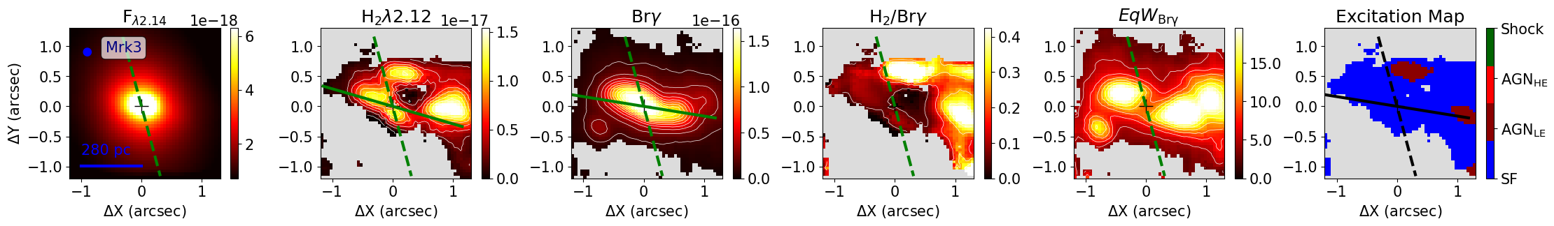
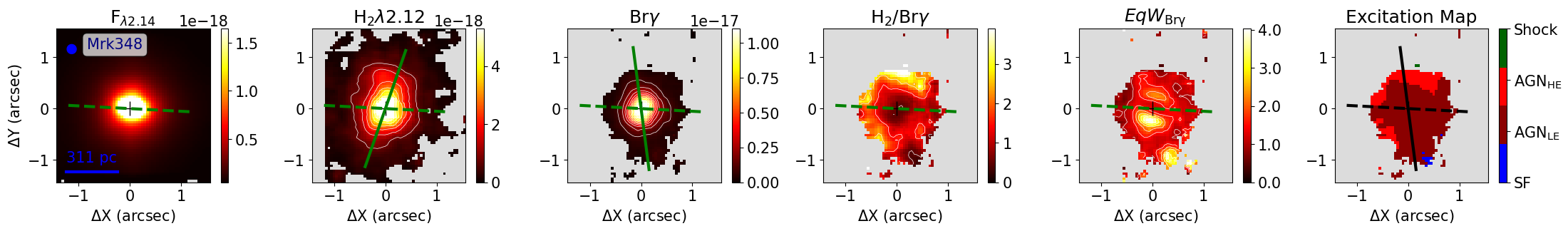
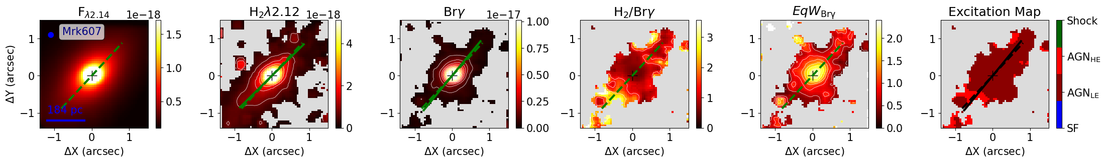
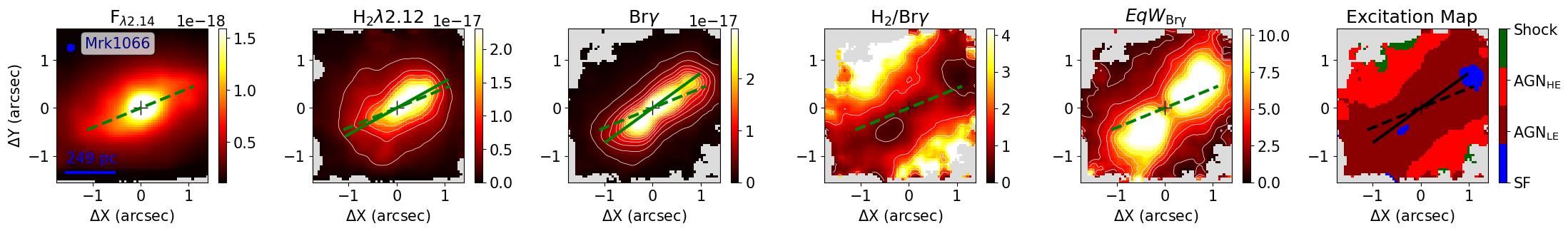
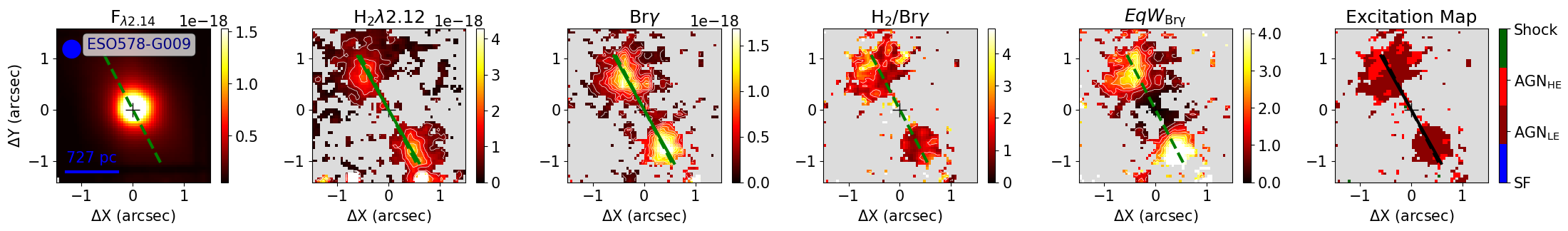
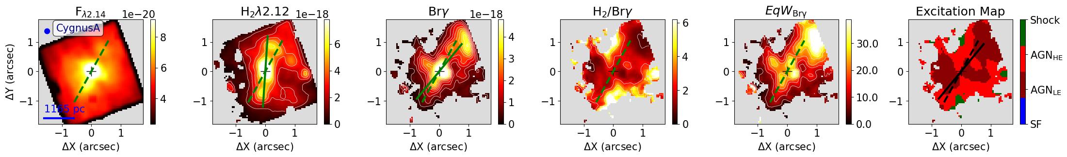
Figure 1: continued.

In Figure 1 we show the X-ray luminosity and redshift distribution of the galaxies of our sample. We divide the sample into type 1 (blue-dashed line) and type 2 (red-continuous line) as in the Table 1. To test whether the distributions for the type 1 and type 2 are drawn from the same underlying distribution, we use the Kolmogorov-Smirnov (K-S) test and compute the probability of the null hypothesis ($P_{\rm KS}$). $P_{\rm KS}<0.05$ implies that the null hypothesis, that the two distributions are drawn from the same underlying distribution, is rejected at a confidence level of 95 per cent. We find high values of $P_{\rm KS}$ for both $L_{\rm X}$ ($P_{\rm KS}=0.75$) and $z$ ($P_{\rm KS}=0.24$) distributions, meaning that the type 1 and type 2 AGN in our sample most likely follow similar distributions in these two parameters. As type 1 and 2 AGN follow the same distributions in terms of X-ray luminosity and redshift, we compare these sub-samples in terms of other physical properties in the following sections.

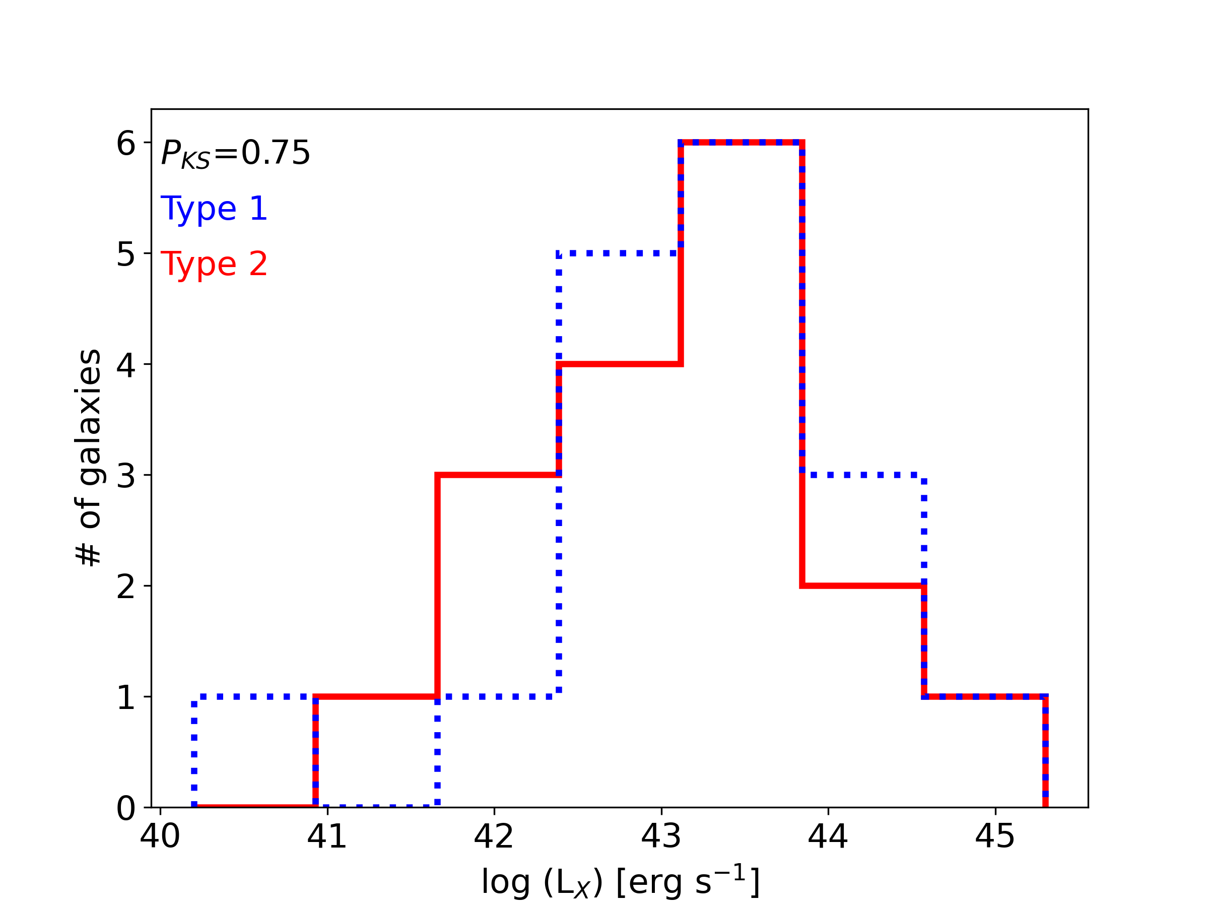
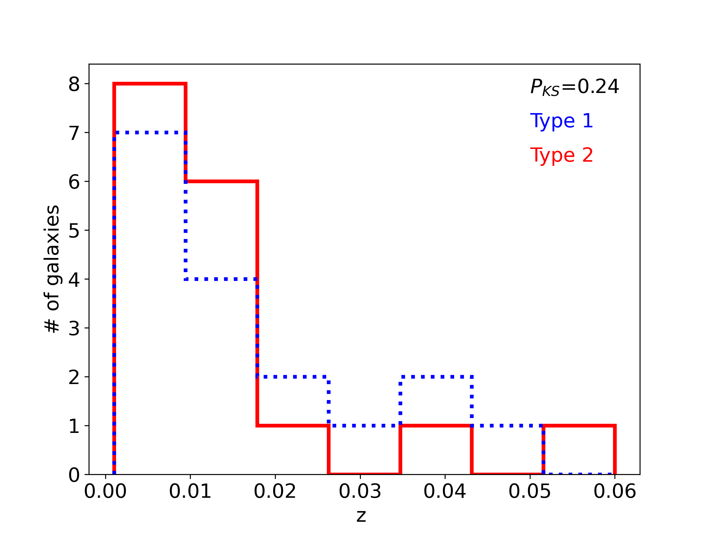
Figure 1: X-ray luminosity (top) and redshift (bottom) distributions of our sample, divided in type 1 (dashed-blue lines) and type 2 (continuous-red lines) AGN. In each panel, we show the probability of the null hypothesis ($P_{\rm KS}$) that type 1 and type 2 AGN follow similar distributions computed using the Kolmogorov-Smirnov test. The $P_{\rm KS}$ values indicate that type 1 and type 2 AGN of our sample do not follow distinct distributions in terms of $L_{\rm X}$ and $z$.

2.2 Observations, Data Reduction and Measurements

The observations were carried out with the NIFS instrument (McGregor et al., 2003) on the Gemini North Telescope from 2006 to 2019. NIFS has a square field of view of $3\aas@@fstack{\prime\prime}0\times 3\aas@@fstack{\prime\prime}0$, divided into 29 slices with an angular sampling of 0$\aas@@fstack{\prime\prime}$103$\times$0$\aas@@fstack{\prime\prime}$042. At the distances of the galaxies of our sample, the NIFS field of view varies from 60$\times$60 pc² to 3.5$\times$3.5 kpc². Most of the observations (34/36) used Adaptive Optics (AO) by coupling NIFS with the ALTtitude conjugate Adaptive optics for the InfraRed (ALTAIR) system. Only NGC 1125 and ESO578-G009 were observed without AO. The resulting angular resolutions are shown in Table 1 and are in the range 0$\aas@@fstack{\prime\prime}$11–0$\aas@@fstack{\prime\prime}$44. Distinct observational strategies were used during the observations, which include the use of K or K_long gratings and spatial dithering, resulting in different spatial and spectral coverage among galaxies. The spectral resolving power of NIFS in the K band is $R\approx 5290$. Telluric standard stars were observed just before and/or after the observations of each galaxy.

The data reduction followed the standard procedures (e.g., Riffel et al., 2017) using the gemini iraf package, including the trimming of the images, flat-fielding, cosmic ray rejection, sky subtraction, wavelength and s-distortion calibrations, removal of the telluric absorptions using the spectra of the telluric standard star and flux calibration by interpolating a black body function to the spectrum of the telluric standard. Finally, the data cubes were created at an angular sampling of 0$\aas@@fstack{\prime\prime}$05$\times$0$\aas@@fstack{\prime\prime}$05 for each individual exposure and median combined using a sigma clipping algorithm to eliminate bad pixels and remaining cosmic rays and using the peak of the continuum emission of the galaxy as reference to perform the astrometry among the individual data cubes.

Results on gas emission properties of individual sources have already been published for 22 galaxies of our sample based on the K-band data used here. The references to these studies are shown in Tab. 1.

The K-band spectra of nearby active galaxies show plenty of H₂ emission lines and usually also present strong Br$\gamma$ emission (e.g. Riffel et al., 2006). To obtain the emission-line flux distributions, we integrated the fluxes within a spectral window of 1500 km s^-1 width centred at each emission line, after subtraction of the contribution of the underlying continuum fitted by a third order polynomial, similarly to the procedure adopted in Storchi-Bergmann et al. (2009). Our spectral window choice is very conservative, as the near-IR line widths in nearby galaxies are commonly much narrower than 1500 km s^-1 and so our choice warrants that we are computing the total line fluxes. To minimize the effect of noise, we followed Liu et al. (2013) and first fitted each emission line by a combination of three Gaussian curves and the continuum by a linear equation using the ifscube code (Ruschel-Dutra, 2020). For type 1 AGN, we included an additional Gaussian to account for the broad Br$\gamma$ component. Before computing the fluxes of Br$\gamma$ in type 1 objects, we subtracted the contribution of this component and thus all measurements presented in this paper are for the narrow line components.

The fitting routine starts by modelling the spaxel corresponding to the peak of the continuum emission, using initial guesses for the centroid velocity and velocity dispersion of each component provided by the user. Then the ifscube code performs the fitting of the neighboring spaxles following a spiral loop and using the parameters from spaxels located at distances smaller than 0$\aas@@fstack{\prime\prime}$25 from the fitted spaxel as optimized guesses (as defined by the refit parameter). As mentioned above, we allow up to three Gaussian components to fit each line profile (4 for the Br$\gamma$ line in Sy 1), but the code finds the minimum number of Gaussians to reproduce the profiles by setting the initial guesses for the amplitudes of the unnecessary Gaussian functions to zero. The fit of multi Gaussians has no physical motivation, it merely aims at reproducing the observed profiles. The emission-line flux distributions measured directly from the observed data cubes are consistent with those obtained from the fits of the line profiles, but the direct measurements produce noisier maps, as already discussed in Liu et al. (2013).

3 Results

3.1 Emission-line flux distributions and line-ratio maps

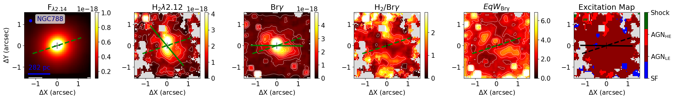
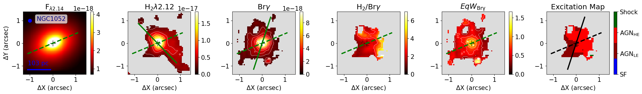
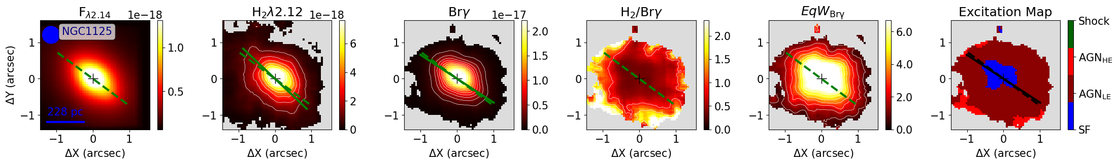
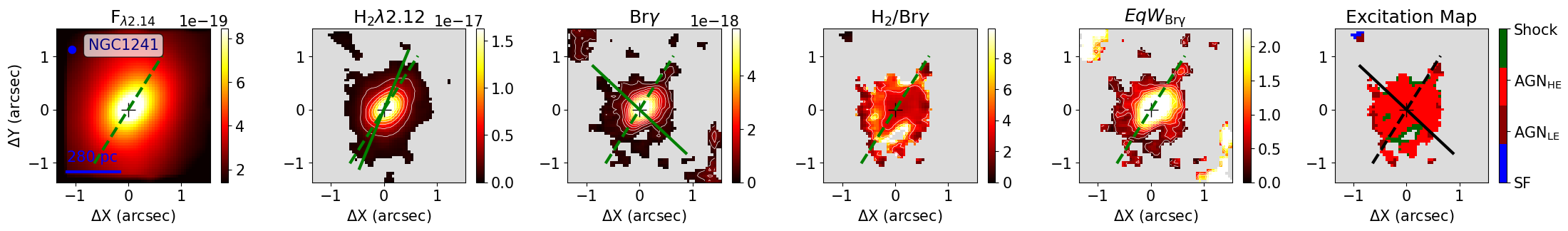
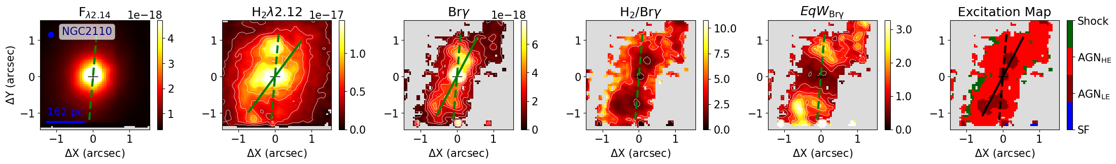
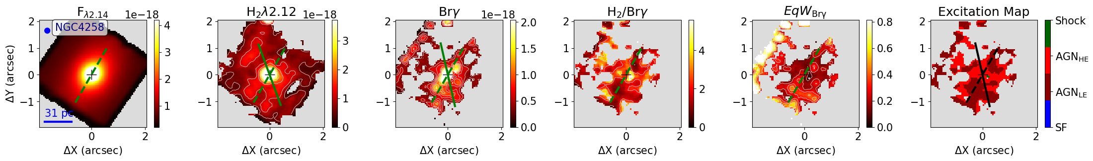
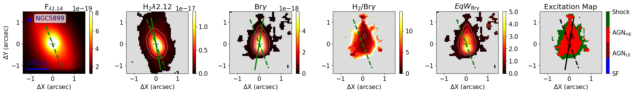
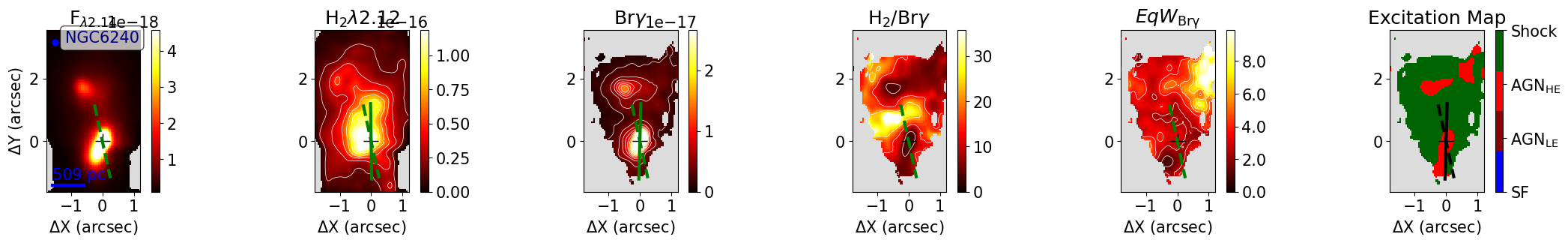
Figure 10: Maps for type 2 AGN. From left to right: K-band continuum obtained within a spectral window of 100 Å centred at 2.14 $\mu$m, H${}_{2}\,2.1218\,\mu$m flux distribution, Br$\gamma$ flux distribution, H₂/Br$\gamma$ ratio map, Br$\gamma$ equivalent width map and excitation map. The color bars show the continuum in units of erg s^-1 cm^-2 Å^-1 spaxel^-1, the emission-line fluxes in erg s^-1 cm^-2 spaxel^-1 and the Br$\gamma$ equivalent width in Å. The excitation map identifies the regions with typical $H_{2}$/Br$\gamma$ values for star forming galaxies (SF: H₂/Br$\gamma<0.4$), AGN with low excitation (AGN_LE: $0.4\leq$ H₂/Br$\gamma<2$) and high excitation (AGN_HE: $2\leq$ H₂/Br$\gamma<6$) and higher line ratios, usually observed in shock dominated objects (Shock: H₂/Br$\gamma>6$). In each row, the name of the galaxy is identified in the continuum image, the filled circle corresponds to the angular resolution of the data, the spatial scale is shown in the bottom-left corner of the continuum image and the cross marks the position of the peak of the continuum emission. The dashed line indicates the orientation of the galaxy major axis obtained from the Hyperleda database. The continuous line on the flux maps shows the orientation of the emission-line flux distributions. The continuous line on the excitation map shows the orientation of the Br$\gamma$ emission. The gray regions indicate locations where the emission lines are not detected within 2$\sigma$ above the continuum noise.

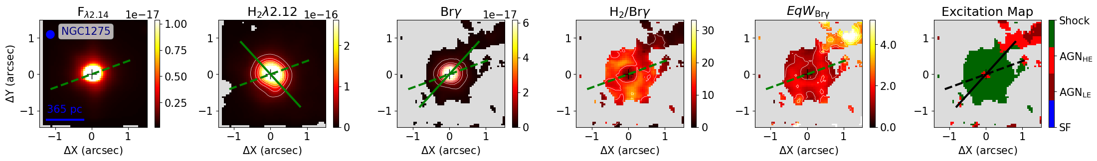
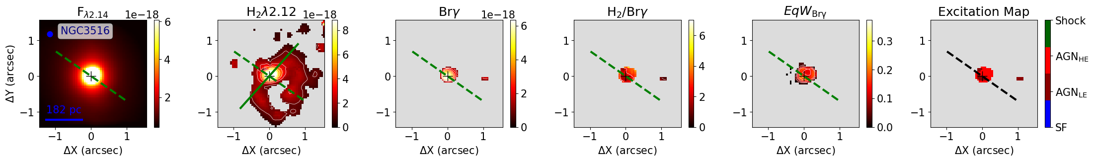
Figure 2: Maps for type 1 AGN. Same as Fig. 10, but for type 1 AGN.

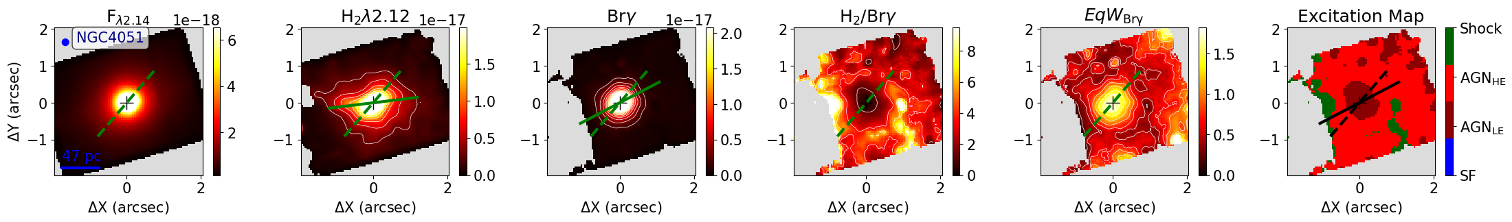
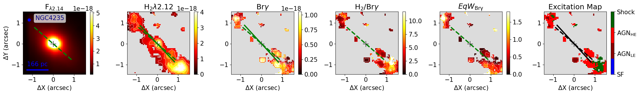
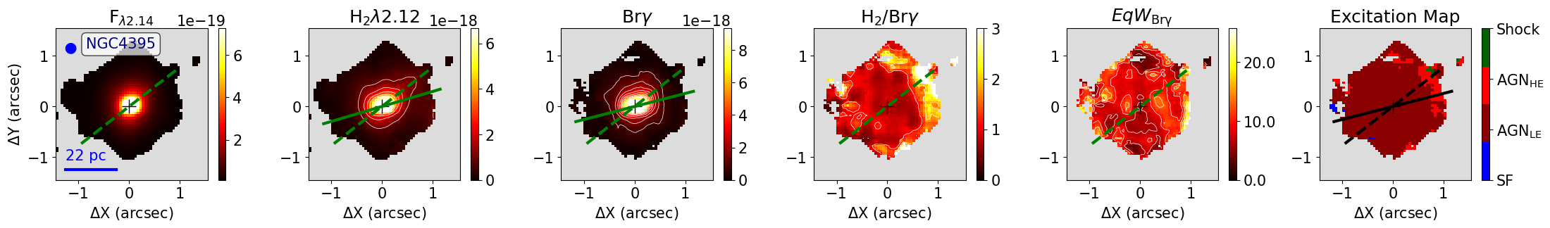
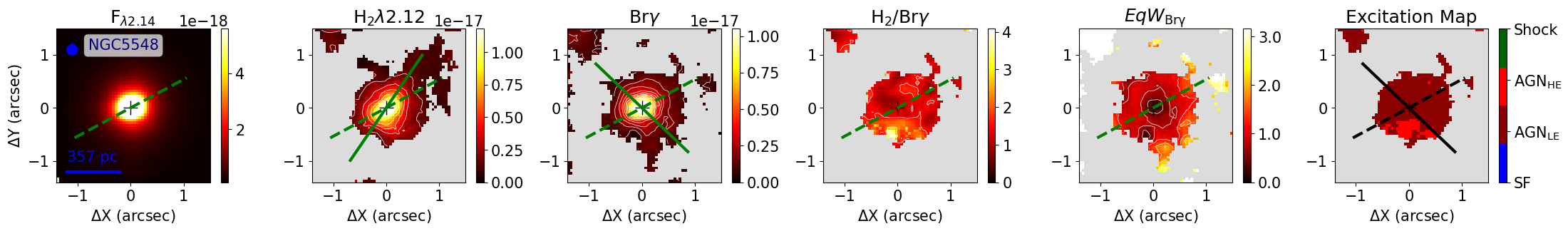
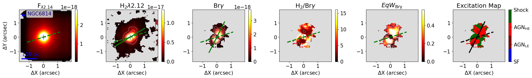
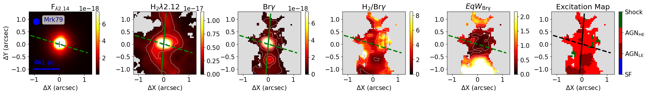
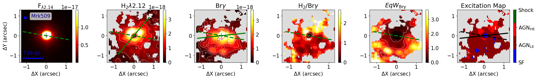
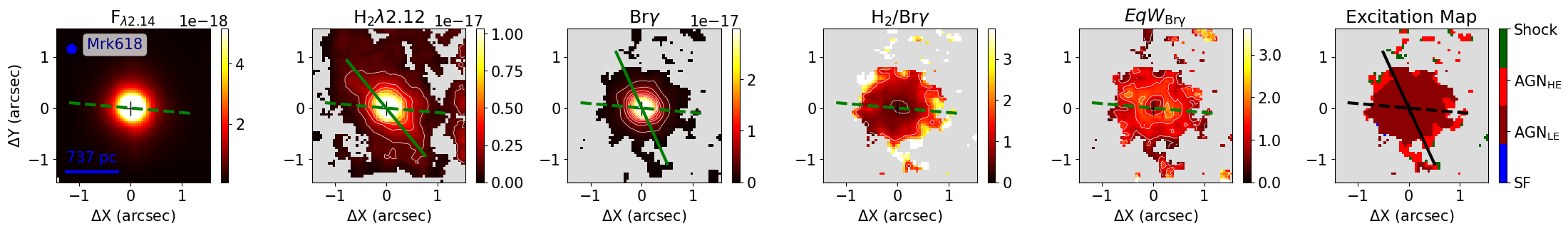
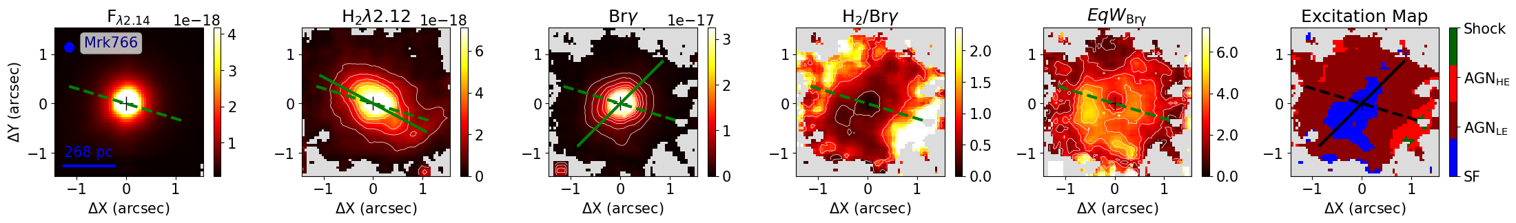
Figure 2: continued.

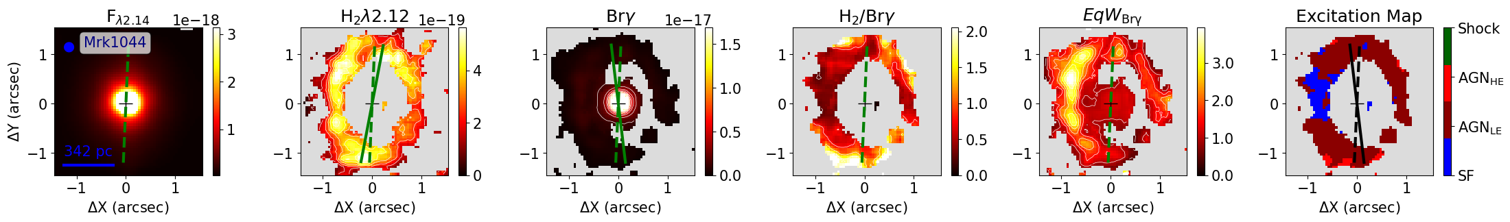
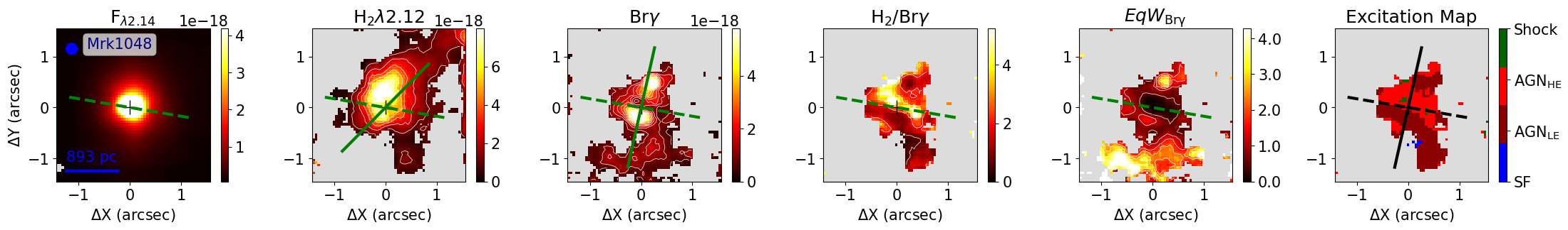
Figure 2: continued.

In Figures 2 and  3 we present examples of maps constructed from the Gemini NIFS data measurements, comprising: the continuum, H${}_{2}\,2.1218\,\mu$m and Br$\gamma$ flux distributions, the H${}_{2}\,2.1218\,\mu$m/Br$\gamma$ ratio map and Br$\gamma$ equivalent width ($EqW$) map for selected type 2 and type 1 AGN, respectively. The maps for the other galaxies are shown in Figures 10 and  2 of the Appendix. We masked out regions where the amplitude of the line profile was smaller than three times the standard deviation of the continuum next to each line profile. The galaxies NGC 3393 (Sy 2) and Mrk 352 (Sy 1) do not present extended line emission and thus we do not show their corresponding maps. All other galaxies show extended emission in both H₂ and Br$\gamma$ emission lines. The only exception is NGC 3516, for which the Br$\gamma$ emission is seen only from the unresolved nucleus.

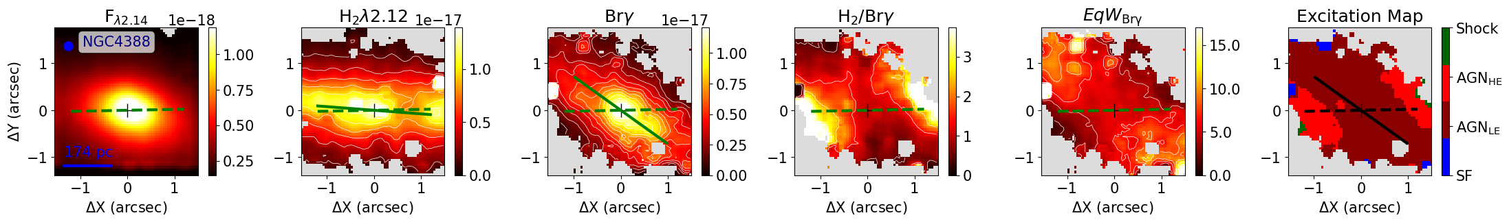
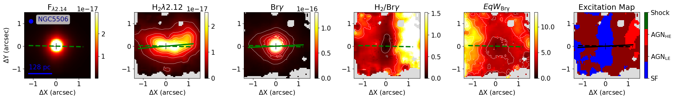
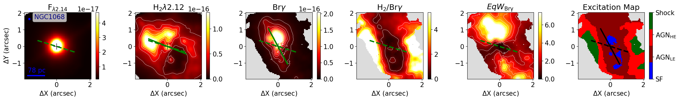
Figure 2: Selected maps for type 2 AGN. From left to right: K-band continuum obtained within a spectral window of 100 Å centred at 2.14 $\mu$m, H${}_{2}\,2.1218\,\mu$m flux distribution, Br$\gamma$ flux distribution, H₂/Br$\gamma$ ratio map, Br$\gamma$ equivalent width map and excitation map. The color bars show the continuum in units of erg s^-1 cm^-2 Å^-1 spaxel^-1, the emission-line fluxes in erg s^-1 cm^-2 spaxel^-1 and the Br$\gamma$ equivalent width in Å. The excitation map identifies with different colors the regions with typical $H_{2}$/Br$\gamma$ values for: star forming regions (SF: H₂/Br$\gamma<0.4$), low excitation AGN (AGN_LE: $0.4\leq$ H₂/Br$\gamma<2$) and high excitation AGN (AGN_HE: $2\leq$ H₂/Br$\gamma<6$) and shock-dominated objects (Shock: H₂/Br$\gamma>6$). In each row, the name of the galaxy is identified in the continuum image, the filled circle corresponds to the angular resolution, the spatial scale is shown in the bottom-left corner of the continuum image and the cross marks the position of the peak of the continuum emission. The dashed line indicates the orientation of the galaxy major axis obtained from the Hyperleda database. The continuous line on the flux maps shows the orientation of the emission-line flux distributions. The continuous line on the excitation map shows the orientation of the Br$\gamma$ emission. The gray regions indicate locations where emission lines are not detected above 3 times the continuum noise amplitude (3$\sigma$).

For all galaxies, north is up and east is to the left.

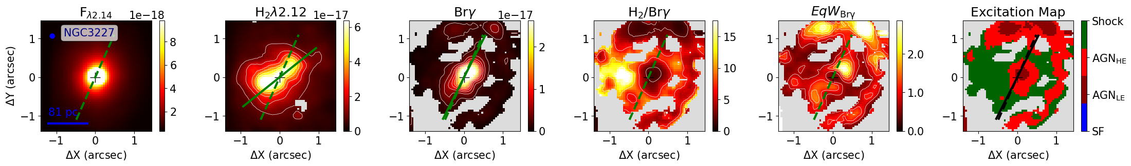
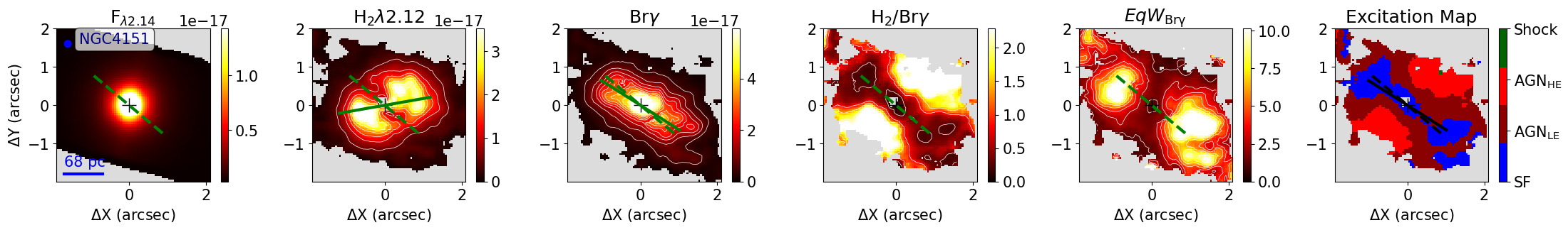
Figure 3: Examples of maps for type 1 AGN. Same as Fig. 2, but for type 1 AGN.

3.1.1 Flux distributions

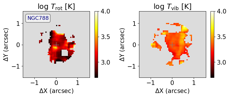
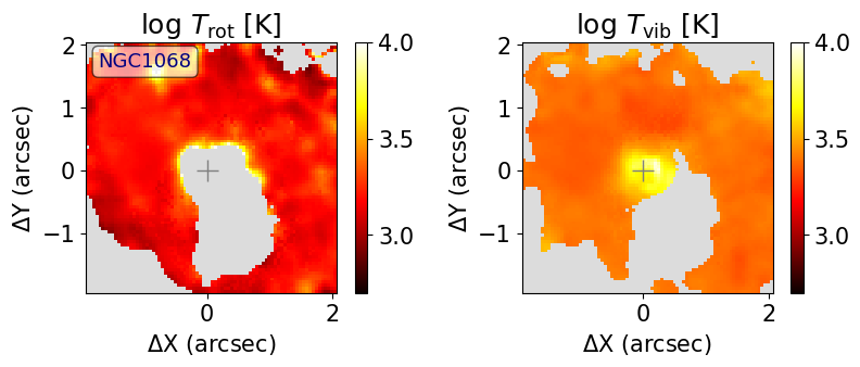
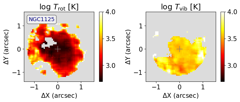
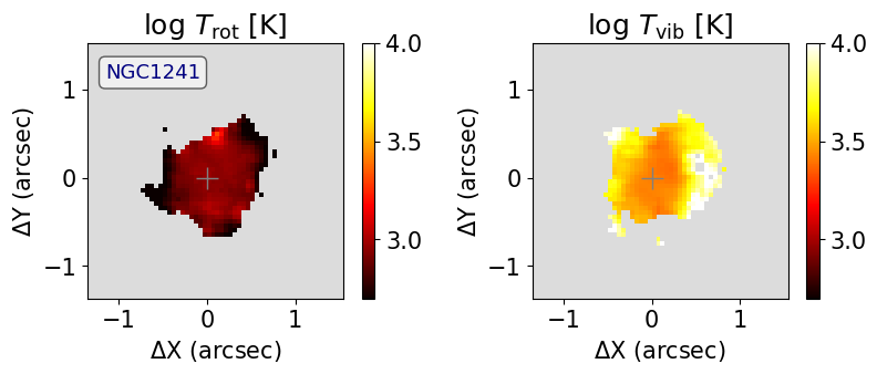
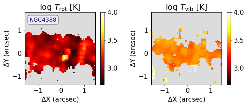
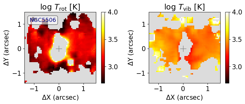
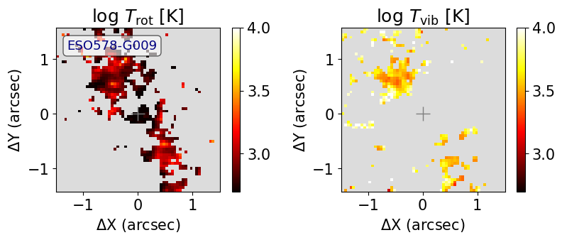
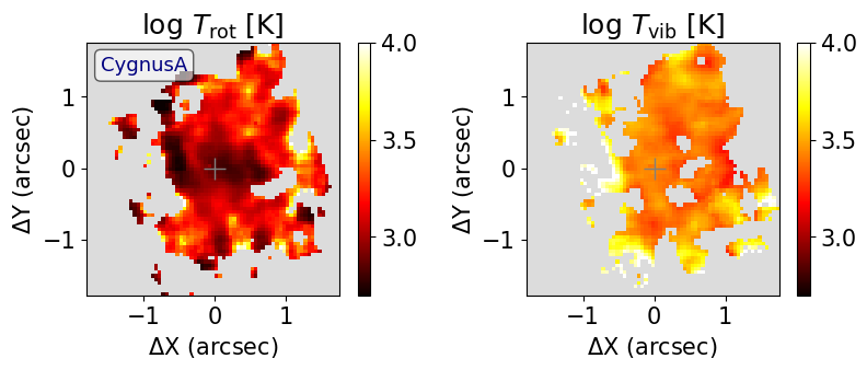
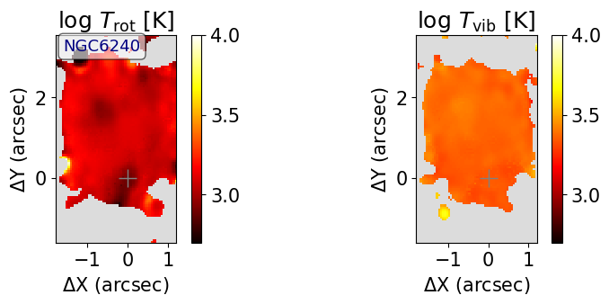
Figure 3: H₂ rotational and vibrational temperatures for type 2 in our sample calculated according to Eqs. 3 and 4. The gray regions indicate locations where at least one of the H₂ emission lines is not detected within 2$\sigma$ above the continuum noise. The colorbar shows the temperatures in logarithmic scale in units of K.

The emission-line flux distributions present a wide variety of structures in both Br$\gamma$ and H₂ emission. In most galaxies, the H₂ emission is more extended than the Br$\gamma$ and the peak emission of both lines is observed at the galaxy nucleus. Other structures observed in the gas distribution comprise: nuclear spirals seen in molecular gas (e.g. Mrk 79); galaxies in which both H₂ and Br$\gamma$ emission are seen mainly along the major axis of the large scale disk (e.g. NGC 4235); galaxies in which the H₂ and Br$\gamma$ emission are distributed along distinct orientations (e.g. NGC 4388); ring-like structures (e.g. Mrk 1044); galaxies with elongated H₂ emission and round Br$\gamma$ flux distribution (e.g. Mrk 766), among other emission structures. There is no clear difference between the emission-line flux distributions of type 1 and type 2 AGN. A qualitative inspection of the H₂ and Br$\gamma$ flux maps in each object (Figs. 2, 3, 10 and 2) shows that the Br$\gamma$ usually traces a more collimated emission, while the H₂ emission spreads more over the whole field of view. This result is consistent with previous studies where the H₂ and ionised gas have been shown to present distinct flux distributions and kinematics (Riffel et al., 2018; Schönell et al., 2019).

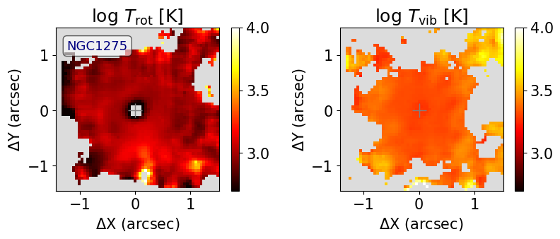
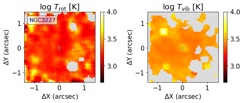
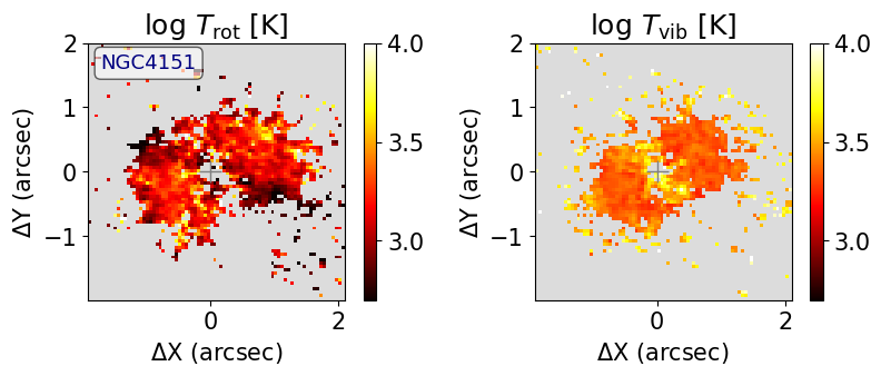
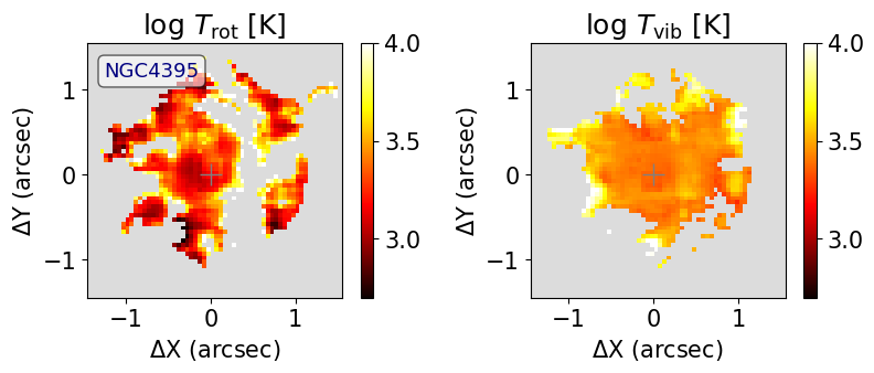
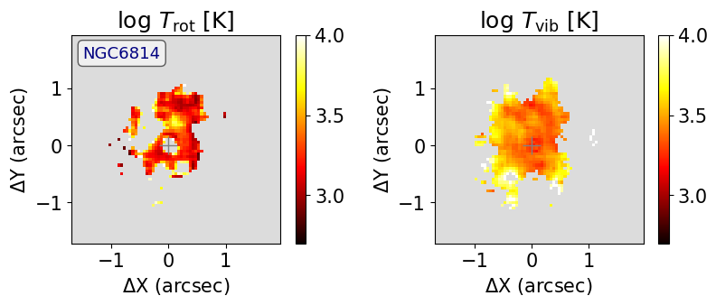
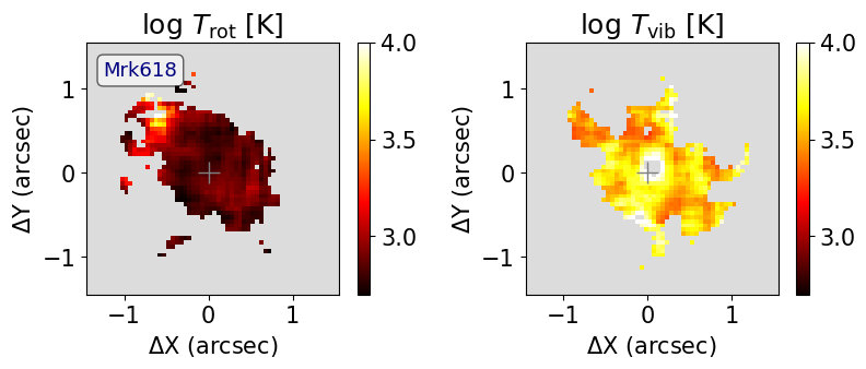
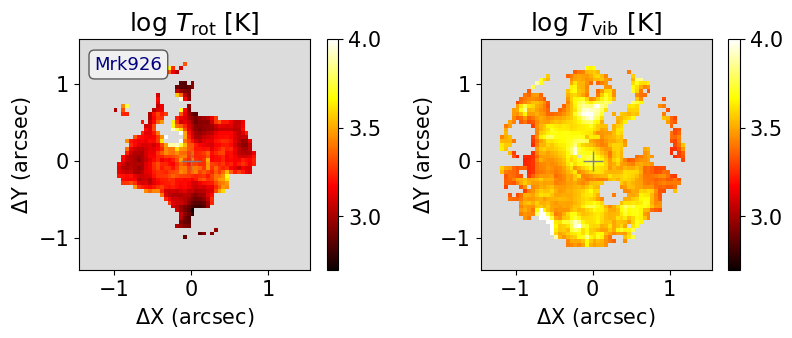
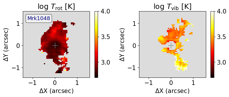
Figure 4: Same as 3, but for type 1 AGN.

We compute the radii that contain 50 % of the total flux ($R_{\rm 50}$) of H₂ 2.1218$\mu$m and Br$\gamma$ emission lines. Although this parameter can be affected by projection effects if the H₂ and Br$\gamma$ emission originate from distinct spatial locations in individual targets, the $R_{\rm 50}$ is useful to compare the H₂ and Br$\gamma$ emission in the whole sample. The corresponding $R_{\rm 50}$ values for H₂ and Br$\gamma$ are shown in Table 2 and Figure 4 shows the comparison between $R_{\rm 50H2}$ and $R_{\rm 50Br\gamma}$. The Br$\gamma$ flux distribution is more concentrated than that of H₂ and the $R_{\rm 50}$ for the H₂ is on average 56 % larger than that of Br$\gamma$.

We use the cv2.moments python package to compute the moments and orientation of the H₂ and Br$\gamma$ flux distributions. The orientations are shown as the continuous lines in the flux maps of Figs. 2, 3, 10 and 2. The position angles (PAs) are listed in Table 2, together with the orientation of the major axis of the galaxy obtained from the Hyperleda database (Paturel et al., 2003), measured from the 25 mag arcsec² isophote in a B-band image. We performed Monte Carlo simulations with 100 iterations each to compute the uncertainties, by adding random noise with amplitude of the 20th percentile flux value of the corresponding map. The listed uncertainties in Tab. 2 correspond to the standard deviation of the mean of the simulations.

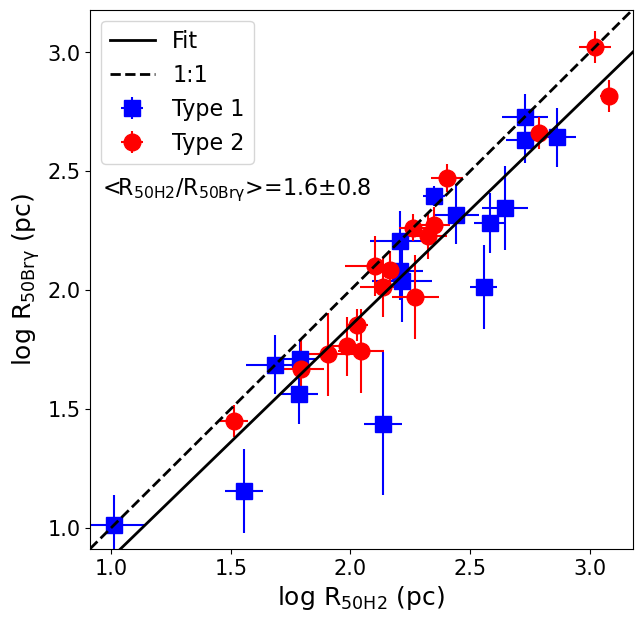
Figure 4: Comparison of the radii that contain 50 % of the total flux of H₂2.1218 $\mu$m and Br$\gamma$. The dashed line shows the 1:1 relation and the continuous line shows the best fit of the data by a first order polynomial, given by $\log{R_{\rm 50\,Br\gamma}}=(0.98\pm 0.20)\times\log{R_{\rm 50\,H_{2}}}-(0.10\pm 0.44)$.

We have compared the PA offset ($\Delta$PA) between the major axis of the large scale disk and the orientation of the Br$\gamma$ and H₂ flux distributions. Although the orientations of both flux distributions vary, the K-S test ($P_{\rm KS}=0.97)$ indicates the distributions of the corresponding $\Delta$PA for Br$\gamma$ and H₂ are not distinct. $\rm\Delta PA>30^{\circ}$ is usually used as a threshold to determine whether the stellar and gas disks are misaligned (Jin et al., 2016). We find $\Delta$PA larger than this value in 15 galaxies (42 %) for the Br$\gamma$ and in 16 galaxies (44 %) for H₂. These fractions are higher than those between the kinematic position angle of the stellar velocity field in the inner 3${}^{\prime\prime}\times$3^′′ and the major axis of the large scale disk, of $\sim$18 % (Riffel et al., 2017), suggesting an origin in non-circular motions in the gas. The distributions of the $\Delta$PA between the orientation of the H₂ and Br$\gamma$ flux distributions (PA_H2-PA_Brγ) for type 1 and type 2 AGN are similar. We find $\rm\Delta PA>30^{\circ}$ for 15 galaxies (45 %). 3 galaxies (NGC 1275, NGC 5548 and Mrk 766) of these show $\rm\Delta PA>60^{\circ}$, for which the H₂ emission is observed mainly along the major axis of the galaxy.

Table 2: (1) Galaxy name, (2) position angle of the large scale disk from Hyperleda database, (3) H₂ and (4) and Br$\gamma$ (4) position flux distribution position angles, (5) and (6) radii that contain half of the total flux of H₂ 2.1218$\mu$m and Br$\gamma$. All angles are measured east of north.

Galaxy	$\Psi_{0}$	PA${}_{\rm H_{2}}$	PABrγ	$R_{\rm 50H_{2}}$	$R_{\rm 50Br\gamma}$
	(deg)	(deg)	(deg)	(pc)	(pc)
(1)	(2)	(3)	(4)	(5)	(6)
type 2
NGC788	108.1	39.8 $\pm$ 1.6	89.4 $\pm$ 3.2	254 $\pm$ 42	296 $\pm$ 42
NGC1052	112.7	44.0 $\pm$ 1.8	162.0 $\pm$ 7.7	62 $\pm$ 15	46 $\pm$ 15
NGC1068	72.7	68.3 $\pm$ 1.2	28.3 $\pm$ 0.6	106 $\pm$ 11	71 $\pm$ 11
NGC1125	53.5	46.5 $\pm$ 1.4	56.7 $\pm$ 1.2	137 $\pm$ 34	102 $\pm$ 34
NGC1241	147.7	157.7 $\pm$ 4.6	46.9 $\pm$ 0.7	126 $\pm$ 42	126 $\pm$ 42
NGC2110	175.1	143.4 $\pm$ 2.2	152.5 $\pm$ 0.9	145 $\pm$ 24	121 $\pm$ 24
NGC4258	150.0	20.3 $\pm$ 2.6	13.2 $\pm$ 7.5	32 $\pm$ 4	28 $\pm$ 4
NGC4388	91.1	85.6 $\pm$ 1.0	54.3 $\pm$ 0.8	183 $\pm$ 26	183 $\pm$ 26
NGC5506	88.7	94.9 $\pm$ 1.3	92.8 $\pm$ 4.3	96 $\pm$ 19	57 $\pm$ 19
NGC5899	20.8	10.3 $\pm$ 1.0	170.7 $\pm$ 1.7	80 $\pm$ 26	53 $\pm$ 26
NGC6240	12.2	0.9 $\pm$ 0.7	178.5 $\pm$ 0.8	610 $\pm$ 76	458 $\pm$ 768
Mrk3	15.0	73.7 $\pm$ 1.3	80.9 $\pm$ 1.2	210 $\pm$ 42	168 $\pm$ 42
Mrk348	87.0	160.8 $\pm$ 2.2	7.5 $\pm$ 5.9	186 $\pm$ 46	93 $\pm$ 46
Mrk607	137.3	134.8 $\pm$ 1.2	140.6 $\pm$ 2.2	110 $\pm$ 27	55 $\pm$ 27
Mrk1066	112.3	118.8 $\pm$ 1.5	126.0 $\pm$ 0.3	224 $\pm$ 37	186 $\pm$ 37
ESO578-G009	27.6	29.9 $\pm$ 0.6	29.3 $\pm$ 0.7	1199 $\pm$ 109	654 $\pm$ 109
CygnusA	151.0	176.1 $\pm$ 1.8	140.6 $\pm$ 1.0	1049 $\pm$ 174	1049 $\pm$ 174
type 1
NGC1275	110.0	42.2 $\pm$ 6.1	137.9 $\pm$ 2.2	164 $\pm$ 54	109 $\pm$ 54
NGC3227	156.0	128.8 $\pm$ 3.1	153.1 $\pm$ 2.2	60 $\pm$ 12	36 $\pm$ 12
NGC3516	55.0	138.0 $\pm$ 4.0	–	$\pm$ 27	27 $\pm$ 27
NGC4051	139.4	96.9 $\pm$ 1.5	117.4 $\pm$ 4.6	35 $\pm$ 7	14 $\pm$ 7
NGC4151	50.0	100.0 $\pm$ 1.0	57.5 $\pm$ 0.4	61 $\pm$ 10	51 $\pm$ 10
NGC4235	49.0	43.4 $\pm$ 0.5	42.6 $\pm$ 0.6	224 $\pm$ 24	249 $\pm$ 24
NGC4395	127.8	106.4 $\pm$ 3.2	104.3 $\pm$ 5.2	10 $\pm$ 4	10 $\pm$ 4
NGC5548	118.2	146.0 $\pm$ 3.8	46.2 $\pm$ 2.3	160 $\pm$ 53	160 $\pm$ 53
NGC6814	107.6	121.2 $\pm$ 1.3	153.2 $\pm$ 1.3	48 $\pm$ 16	48 $\pm$ 16
Mrk79	73.0	176.2 $\pm$ 3.9	171.9 $\pm$ 35.1	276 $\pm$ 69	207 $\pm$ 69
Mrk509	80.0	139.4 $\pm$ 5.1	96.3 $\pm$ 4.3	536 $\pm$ 107	428 $\pm$ 107
Mrk618	85.0	39.4 $\pm$ 2.2	24.8 $\pm$ 3.9	442 $\pm$ 110	221 $\pm$ 110
Mrk766	73.1	62.0 $\pm$ 1.4	135.1 $\pm$ 1.1	160 $\pm$ 40	120 $\pm$ 40
Mrk926	104.1	71.7 $\pm$ 4.2	104.0 $\pm$ 2.9	730 $\pm$ 146	438 $\pm$ 146
Mrk1044	177.5	169.2 $\pm$ 2.2	6.5 $\pm$ 7.9	359 $\pm$ 51	102 $\pm$ 51
Mrk1048	80.3	135.4 $\pm$ 1.5	167.4 $\pm$ 3.0	536 $\pm$ 134	536 $\pm$ 134
MCG+08-11-01	90.0	163.6 $\pm$ 1.3	16.0 $\pm$ 2.4	383 $\pm$ 63	191 $\pm$ 63

3.1.2 Line ratios

The H${}_{2}\,2.1218\,\mu$m/Br$\gamma$ emission-line ratio is commonly used to investigate the main source of the H₂ excitation (Reunanen et al., 2002; Rodríguez-Ardila et al., 2004; Rodríguez-Ardila et al., 2005; Storchi-Bergmann et al., 2009; Riffel et al., 2010a, 2014; Riffel et al., 2013a; Riffel, 2020b; Colina et al., 2015; Schönell et al., 2014; Schönell et al., 2019; Dahmer-Hahn et al., 2019b; Fazeli et al., 2020). Small values ($\rm H_{2}/Br\gamma\lesssim 0.4$) are usually observed in H ii regions and star forming galaxies, while AGN present $\rm 0.4\lesssim H_{2}/Br\gamma\lesssim 6.0$ and higher values are usually observed in LINERs and shock-dominated regions (e.g. Riffel et al., 2013a; Colina et al., 2015; Riffel et al., 2021). In the near-IR the line ratio limits are empirical and their excitation mechanisms are less understood than those of the optical lines (e.g. Rodríguez-Ardila et al., 2004; Rodríguez-Ardila et al., 2005). However, it is worth mentioning that the H₂/Br$\gamma$ line ratio can be affected by the geometry of the Hii region (Puxley et al., 1990) and the velocity of the shock (Wilgenbus et al., 2000). Both properties affect the dissociation of the H₂ molecule, making the fraction of H₂, and the H₂/Br$\gamma$ ratio, to change. The H₂/Br$\gamma$ maps for our sample (Figs. 2, 3, 10 and 2) show values ranging from nearly zero, as seen in the rings of star forming regions of Mrk 1044 and for NGC 4151 – in which the H₂ emission decreases due to the dissociation of the molecule by the strong AGN radiation field (e.g. Storchi-Bergmann et al., 2009) – to values of up to $\rm H_{2}/Br\gamma\sim 30$ for NGC 1275, where the H₂ emission originates in shocks produced by AGN winds (Riffel, 2020a).

We build excitation maps (fifth column of Figs. 2, 3, 10 and 2) to spatially locate the regions where different excitation mechanisms may be occurring. All galaxies present spaxels dominated by AGN excitation ($0.4<\rm H_{2}/Br\gamma<6$), and in order to map the variation of this excitation, we have divided the AGN regions into low ($0.4\leq\rm H_{2}/Br\gamma<2$) and high excitation ($2\leq\rm H_{2}/Br\gamma<6$). This separation allow us to further investigate the origin of the H₂ emission in the AGN. A similar separation was done in Riffel et al. (2020) to split the high line ratio region in the H₂ 2.1218 $\mu$m/Br$\gamma$ vs. [Fe ii]1.2570 $\mu$m/Pa$\beta$ diagnostic diagram.

Table 3 presents the median H₂/Br$\gamma$ ratio over the whole FoV (H₂/Br$\gamma_{\rm MED}$) for each galaxy of our sample, the median value within $r<125$ pc (H₂/Br$\gamma_{r<125{\rm pc}}$), the nuclear ratio, computed using an aperture with radius equal to the angular resolution of the data for each galaxy (H₂/Br$\gamma_{\rm nuc}$), and the extra-nuclear line ratio, measured as the median value of spaxels located at distances from the galaxy nucleus larger than the angular resolution (H₂/Br$\gamma_{\rm extra}$). The median values of H₂/Br$\gamma$ are within the AGN range for 31 (91 %) galaxies of our sample. The exceptions are NGC 6240, NGC 1275 and Mrk 3 that show H₂/Br$\gamma$ median values of 11.76, 11.10 and 0.17, respectively. The high H₂/Br$\gamma_{\rm MED}$ values are consistent with shocks as the dominant H₂ excitation mechanism (Ilha et al., 2016; Müller-Sánchez et al., 2018a; Riffel, 2020a). The low ratios observed for Mrk 3, NGC 5506 and NGC 4151 may be explained by the dissociation of the H₂ molecule by the AGN radiation field in these galaxies as proposed by previous works (Gnilka et al., 2020; Storchi-Bergmann et al., 2009). As seen in Tab. 3, type 1 and type 2 AGN show similar values of H₂/Br$\gamma$ median values.

We use K-S statistics to test whether the distributions of H₂/Br$\gamma_{\rm MED}$ for type 1 and type 2 AGN are distinct. We find $P_{\rm KS}=0.96$, meaning that likely the H₂/Br$\gamma_{\rm MED}$ distributions of type 1 and type 2 AGN are drawn from the same underlying distribution. However, our observations cover spatial scales from a few tens of pc to a few kpc, and so, for the most distant objects the H₂/Br$\gamma_{\rm MED}$ is dominated by the extra-nuclear regions, while in the closest galaxies, the contribution of the nuclear emission is higher. In order to avoid this problem, we compute the H₂/Br$\gamma$ within the inner 125 pc radius for all objects. This aperture corresponds to the lowest spatial resolution in our sample (for ESO578-G009). For three galaxies (NGC 4258, NGC 4051 and NGC 4395) the FoV is smaller than 125 pc radius and thus, we use the whole FoV to compute the H₂/Br$\gamma$ in these cases. The K-S test indicates again that type 1 and type 2 AGN do not have distinct distributions of H₂/Br$\gamma$ within the inner 125 pc radius. Similarly, we do not find a statistically significant difference in the nuclear H₂/Br$\gamma$ distributions (computed for an aperture corresponding to the angular resolution of the data for each galaxy) for type 1 and type 2 AGN. Finally, we test whether H₂/Br$\gamma$ (median, within 125 pc radius and nuclear) and the hard X-ray luminosity are correlated using the Pearson test, resulting that these parameters do not present a statistically significant correlation.

Table 3: H₂/Br$\gamma$ line ratio: (1) galaxy name, (2) median values of the line ratio for the whole FoV (H₂/Br$\gamma_{\rm MED}$), (3) in the inner $r<125$ pc (H₂/Br$\gamma_{r<125\rm pc}$), (4) wihin the central angular resolution element (H₂/Br$\gamma_{\rm nuc}$) and (5) for spaxels at distances larger than the angular resolution radius (H₂/Br$\gamma_{\rm extra}$).

Galaxy	H2/Br$\gamma_{\rm MED}$	H2/Br$\gamma_{r<125\rm pc}$	H2/Br$\gamma_{\rm nuc}$	H2/Br$\gamma_{\rm extra}$
(1)	(2)	(3)	(4)	(5)
type 2
NGC788	0.96$\pm$0.91	0.82$\pm$0.35	0.53$\pm$0.05	0.96$\pm$0.91
NGC1052	2.32$\pm$1.07	2.32$\pm$1.07	2.15$\pm$0.27	2.36$\pm$1.09
NGC1068	1.78$\pm$3.18	1.30$\pm$3.72	0.54$\pm$0.10	1.79$\pm$3.18
NGC1125	0.78$\pm$0.62	0.39$\pm$0.06	0.38$\pm$0.04	0.88$\pm$0.62
NGC1241	3.11$\pm$2.21	3.21$\pm$1.58	2.67$\pm$0.09	3.18$\pm$2.24
NGC2110	3.61$\pm$1.57	3.15$\pm$1.57	1.36$\pm$0.38	3.65$\pm$1.55
NGC4258	1.84$\pm$0.90	1.84$\pm$0.90	2.59$\pm$1.47	1.81$\pm$0.85
NGC4388	1.25$\pm$1.16	1.31$\pm$0.38	1.15$\pm$0.16	1.26$\pm$1.17
NGC5506	0.51$\pm$0.68	0.43$\pm$0.45	0.09$\pm$0.02	0.51$\pm$0.68
NGC5899	4.35$\pm$4.13	4.27$\pm$4.38	2.40$\pm$0.13	4.41$\pm$4.15
NGC6240	11.78$\pm$7.49	8.55$\pm$4.70	8.65$\pm$3.96	11.95$\pm$7.86
Mrk3	0.17$\pm$0.15	0.07$\pm$0.04	0.04$\pm$0.01	0.18$\pm$0.15
Mrk348	1.30$\pm$0.84	0.89$\pm$0.28	0.56$\pm$0.09	1.34$\pm$0.83
Mrk607	1.06$\pm$0.69	0.93$\pm$0.37	0.51$\pm$0.06	1.08$\pm$0.69
Mrk1066	1.39$\pm$1.51	1.41$\pm$0.55	1.41$\pm$0.16	1.39$\pm$1.51
ESO578-G009	1.60$\pm$1.77	2.97$\pm$0.77	2.17$\pm$1.17	1.59$\pm$1.79
CygnusA	2.06$\pm$1.75	1.92$\pm$0.14	1.93$\pm$0.27	2.08$\pm$1.76
Mean	2.35$\pm$2.58	2.10$\pm$1.96	1.71$\pm$1.94	2.38$\pm$2.62
type 1
NGC1275	11.09$\pm$5.27	12.40$\pm$3.95	7.56$\pm$2.33	11.42$\pm$5.37
NGC3227	5.72$\pm$3.84	5.89$\pm$3.81	1.84$\pm$0.41	5.75$\pm$3.83
NGC3516	2.31$\pm$0.86	2.47$\pm$0.74	2.14$\pm$0.42	2.61$\pm$0.99
NGC4051	3.16$\pm$2.03	3.16$\pm$2.03	0.53$\pm$0.08	3.19$\pm$2.02
NGC4151	0.76$\pm$1.16	0.79$\pm$1.19	0.21$\pm$0.07	0.78$\pm$1.16
NGC4235	3.71$\pm$1.88	3.10$\pm$1.29	–	3.71$\pm$1.88
NGC4395	1.01$\pm$0.88	1.01$\pm$0.88	0.79$\pm$0.06	1.02$\pm$0.89
NGC5548	1.37$\pm$0.48	1.27$\pm$0.33	1.17$\pm$0.14	1.39$\pm$0.49
NGC6814	5.55$\pm$6.00	5.73$\pm$41.48	18.57$\pm$149.12	5.34$\pm$6.45
Mrk79	2.83$\pm$1.61	2.59$\pm$0.79	2.56$\pm$0.74	2.87$\pm$1.66
Mrk509	0.91$\pm$0.64	0.41$\pm$0.60	0.23$\pm$0.19	0.91$\pm$0.63
Mrk618	1.24$\pm$1.97	0.44$\pm$0.04	0.44$\pm$0.04	1.28$\pm$1.99
Mrk766	0.80$\pm$1.02	0.34$\pm$0.12	0.13$\pm$0.04	0.82$\pm$1.03
Mrk926	1.83$\pm$0.80	1.71$\pm$0.19	1.72$\pm$0.28	1.85$\pm$0.82
Mrk1044	0.68$\pm$0.52	0.05$\pm$0.01	–	0.68$\pm$0.52
Mrk1048	1.75$\pm$1.42	3.25$\pm$1.12	3.07$\pm$1.90	1.69$\pm$1.32
MCG+08-11-01	2.19$\pm$2.65	1.01$\pm$0.77	0.70$\pm$0.41	2.31$\pm$2.66
Mean	2.76$\pm$2.57	2.68$\pm$2.96	2.78$\pm$4.59	2.80$\pm$2.62

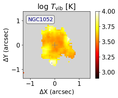
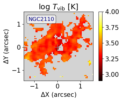
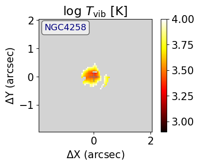
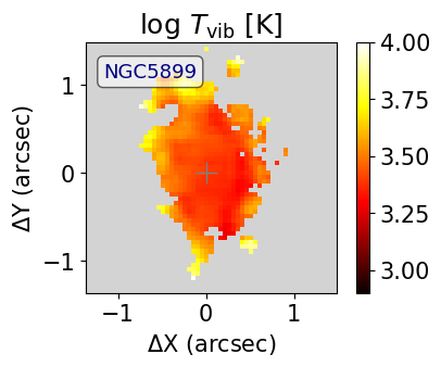
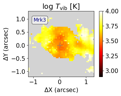
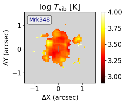
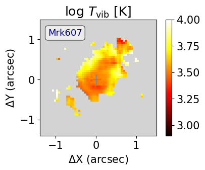
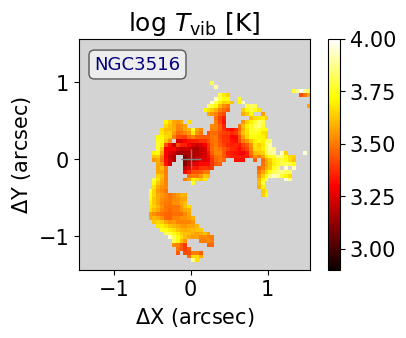
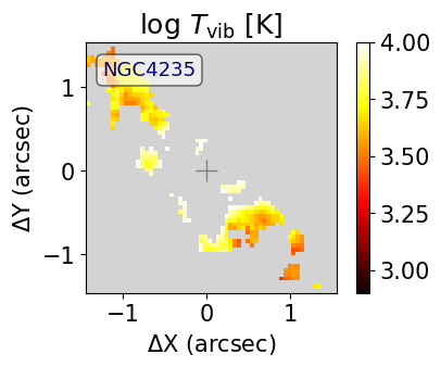
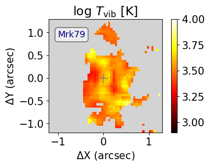
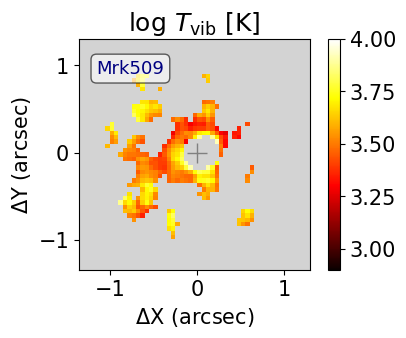
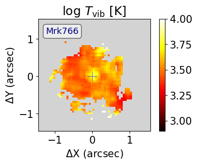
Figure 5: H₂ vibrational for objects where the H₂ 1–0 S(2) line is not detected.

Figure 5 shows the only distinct distributions we found: the H₂/Br$\gamma_{\rm nuc}$ and H₂/Br$\gamma_{\rm extra}$ ones. Using the K-S test we obtain $P_{\rm KS}=0.045$ indicating that the distributions are distinct: on average, the nucleus presents lower H₂/Br$\gamma$ ratios than the extra-nuclear regions.

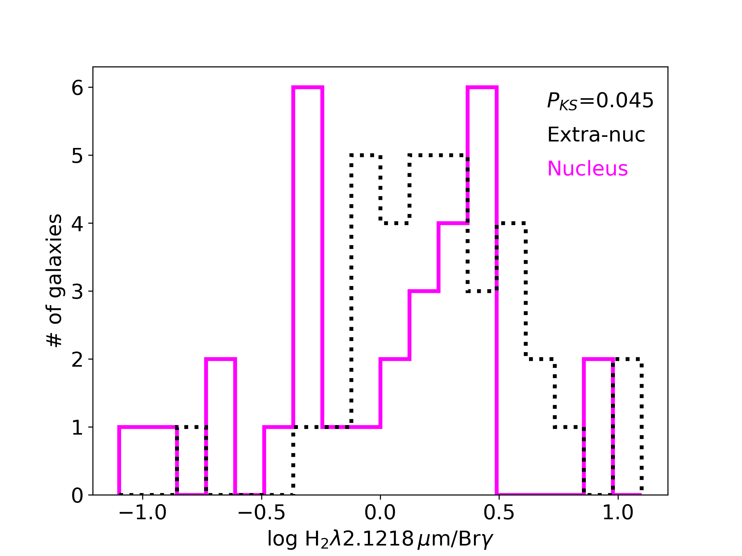
Figure 5: Nuclear (magenta) and extra-nuclear (dotted black) H₂/Br$\gamma$ distributions of the galaxies of our sample.

3.2 Br$\gamma$ Equivalent width maps

The fifth column of Figs. 2, 3, 10 and 2 shows the Br$\gamma$ equivalent width ($EqW_{\rm Br\gamma}$) maps. The emission structures are better seen in the $EqW_{\rm Br\gamma}$ than in the flux distribution maps, as the former measure the emission relative to the continuum. For example, in Mrk 3 (Fig. 10) the $EqW_{\rm Br\gamma}$ map shows knots of emission not easily observed in the Br$\gamma$ flux map. Young ($<$10 Myr) stellar populations present $EqW_{\rm Br\gamma}\gtrsim 50$ Å, as predicted by evolutionary photoionisation models (Dors et al., 2008; Riffel et al., 2009a). All galaxies of our sample clearly show smaller values ($EqW_{\rm Br\gamma}\lesssim 30$ Å) than those predicted for young stellar population models. Even galaxies with known active star-formation, as NGC 6240 (e.g. Keel, 1990; Lutz et al., 2003; Pasquali et al., 2004) and NGC 3227 (Gonzalez Delgado & Perez, 1997; Schinnerer et al., 2000), present low $EqW_{\rm Br\gamma}$ values, which suggest the near-infrared continuum is dominated by the contribution of old stellar populations and the AGN featureless continuum in the nucleus.

Differently from the Br$\gamma$ flux distributions, which usually present the emission peak at the nucleus, the highest values of $EqW_{\rm Br\gamma}$ are seen away from the nucleus in most galaxies of our sample. In addition, a visual inspection of the $EqW_{\rm Br\gamma}$ maps shows a drop in the $EqW_{\rm Br\gamma}$ values at the nucleus. This drop is more prominent in type 1 AGN than in type 2, possibly due to a stronger dilution of the Br$\gamma$ emission by the nuclear continuum.

We measure the $EqW_{\rm Br\gamma}$ values for the nucleus of each galaxy within an aperture corresponding to the angular resolution of the data and compare the $EqW_{\rm Br\gamma}$ distributions of type 1 and type 2 AGN and find that they follow distinct distributions ($P_{\rm KS}=0.011$). Figure 6 shows the $EqW_{\rm Br\gamma}$ distributions for type 1 AGN (in blue) and type 2 (in red) AGN. A slightly higher $P_{\rm KS}$ (0.045) is obtained by comparing the Br$\gamma$ equivalent widths within the same spatial region of all galaxies (125 pc radius) implying the null hypothesis in which type 1 and type 2 AGN follow the same underlying distribution is rejected at the 95 % confidence level. On the other hand, the comparison of the median $EqW_{\rm Br\gamma}$ distributions over the whole FoV results in $P_{\rm KS}=0.465$, meaning that the null hypothesis cannot be rejected and likely type 1 and type 2 AGN originate from the same underlying $EqW_{\rm Br\gamma}$ distribution. The Pearson test shows that $EqW_{\rm Br\gamma}$ does not correlate with $L_{\rm X}$. This result suggests that there is no intrinsic difference between these type 1 and type 2 AGN, just circunstantial due orientation so that, at larger scales, where the central source is not seen, no clear distinction can be made between the two.

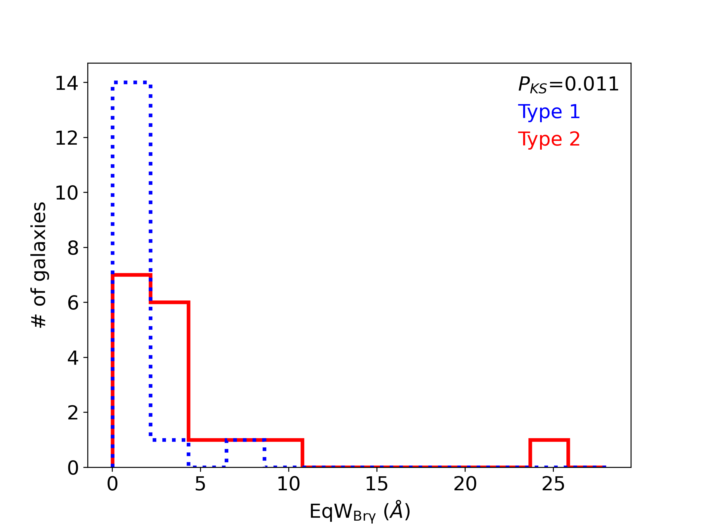
Figure 6: Nuclear Br$\gamma$ equivalent width distributions for the type 1 (dashed-blue lines) and type 2 (continuous-red lines) AGN in our sample. The equivalent widths are measured within apertures corresponding to the angular resolution of the data.

Table 4: Ionised and hot H₂ gas masses and H₂ excitation temperatures. (1) Name of the galaxy; (2 & 3) Hot Molecular and ionised hydrogen masses within the inner 125 pc radius and (4 & 5) in the whole field of view; (6 & 7) H₂ vibrational and rotational temperatures.

Galaxy	$M_{{\rm H_{2}}\,r<\rm 125pc}$	$M_{{\rm H\,II}\,r<125\rm pc}$	$M_{\rm H_{2}\,FoV}$	$M_{\rm HII\,FoV}$	$T_{\rm vib}$	$T_{\rm rot}$
	(101 M⊙)	(104 M⊙)	(101 M⊙)	(104 M⊙)	(K)	(K)
(1)	(2)	(3)	(4)	(5)	(6)	(7)
type 2
NGC788	12.8$\pm$0.5	19.5$\pm$0.6	59.0$\pm$5.6	83.4$\pm$9.2	2149$\pm$80	810$\pm$567
NGC1052	11.0$\pm$1.1	5.7$\pm$1.6	11.9$\pm$1.4	5.8$\pm$1.8	4233$\pm$306	–
NGC1068	202.5$\pm$2.2	193.1$\pm$3.8	288.6$\pm$4.2	222.2$\pm$6.2	2474$\pm$11	1551$\pm$332
NGC1125	21.3$\pm$0.7	64.1$\pm$0.8	41.7$\pm$3.9	94.1$\pm$6.4	3857$\pm$161	1345$\pm$633
NGC1241	34.9$\pm$0.7	13.0$\pm$0.9	51.0$\pm$5.4	19.4$\pm$4.3	3746$\pm$123	832$\pm$753
NGC2110	41.7$\pm$0.8	16.8$\pm$1.0	100.5$\pm$3.1	27.4$\pm$2.1	2512$\pm$23	–
NGC4258	–	–	0.7$\pm$0.1	0.3$\pm$0.1	5132$\pm$2490	–
NGC4388	40.0$\pm$1.1	35.3$\pm$1.5	119.6$\pm$5.8	101.5$\pm$6.4	2725$\pm$33	1065$\pm$593
NGC5506	45.7$\pm$0.7	174.1$\pm$1.4	66.8$\pm$2.0	204.8$\pm$4.3	2746$\pm$24	1154$\pm$358
NGC5899	17.8$\pm$0.8	6.6$\pm$1.1	21.4$\pm$2.4	7.1$\pm$3.5	2853$\pm$76	–
NGC6240	533.0$\pm$1.6	99.0$\pm$2.5	10926.4$\pm$88.5	992.5$\pm$34.2	2339$\pm$3	1247$\pm$74
Mrk3	23.6$\pm$2.7	498.09.5$\pm$4.9	99.6$\pm$8.9	1167.2$\pm$28.3	4953$\pm$139	–
Mrk348	17.6$\pm$0.6	27.3$\pm$0.9	42.6$\pm$6.1	39.4$\pm$4.7	2932$\pm$73	–
Mrk607	7.1$\pm$0.4	11.3$\pm$0.7	12.0$\pm$1.2	13.1$\pm$1.5	4079$\pm$301	–
Mrk1066	57.4$\pm$0.4	68.6$\pm$0.7	228.4$\pm$5.7	270.0$\pm$8.7	2614$\pm$19	–
ESO578-G009	0.4$\pm$0.3	1.2$\pm$1.3	251.6$\pm$37.5	83.0$\pm$19.3	4223$\pm$298	757$\pm$654
CygnusA	51.7$\pm$0.3	32.5$\pm$0.3	2163.2$\pm$63.4	1109.3$\pm$59.2	2777$\pm$32	1352$\pm$410
Mean	67.0$\pm$121.1	74.5$\pm$120.3	852.2$\pm$2494.1	261.7$\pm$393.1	3409$\pm$955	1096$\pm$302
type 1
NGC1275	1170.3$\pm$5.3	150.6$\pm$8.5	2327.5$\pm$56.7	229.8$\pm$20.5	2309$\pm$12	1021$\pm$351
NGC3227	52.1$\pm$1.3	11.5$\pm$1.2	53.7$\pm$1.5	11.8$\pm$1.3	2906$\pm$27	1909$\pm$586
NGC3516	8.7$\pm$2.2	2.0$\pm$0.3	16.2$\pm$2.7	2.1$\pm$1.9	3583$\pm$374	–
NGC4051	–	–	7.4$\pm$0.3	4.7$\pm$0.6	3596$\pm$88	1354$\pm$876
NGC4151	36.9$\pm$1.3	54.7$\pm$1.6	37.8$\pm$1.8	56.8$\pm$2.3	2495$\pm$45	1365$\pm$778
NGC4235	4.0$\pm$0.5	0.2$\pm$0.1	13.7$\pm$1.2	1.9$\pm$0.5	5055$\pm$1425	–
NGC4395	–	–	0.2$\pm$0.1	0.2$\pm$0.1	2866$\pm$70	2075$\pm$656
NGC5548	33.3$\pm$5.5	32.1$\pm$6.8	79.7$\pm$28.5	71.2$\pm$32.8	–	–
NGC6814	7.8$\pm$0.8	1.4$\pm$0.4	8.6$\pm$1.4	1.4$\pm$0.6	3093$\pm$115	1811$\pm$812
Mrk79	52.9$\pm$2.1	23.9$\pm$2.5	195.6$\pm$12.1	61.4$\pm$6.7	3392$\pm$95	–
Mrk509	8.2$\pm$10.1	21.0$\pm$9.3	213.8$\pm$26.0	226.9$\pm$22.3	3539$\pm$320	–
Mrk618	62.5$\pm$8.3	162.8$\pm$10.4	507.1$\pm$58.0	538.0$\pm$82.7	4009$\pm$291	752$\pm$703
Mrk766	23.3$\pm$2.0	112.2$\pm$3.7	60.5$\pm$7.3	166.5$\pm$17.7	3278$\pm$164	–
Mrk926	79.3$\pm$12.5	54.7$\pm$15.2	1340.8$\pm$106.5	507.2$\pm$53.0	3388$\pm$173	1498$\pm$932
Mrk1044	0.1$\pm$0.1	53.5$\pm$4.9	11.5$\pm$3.1	81.7$\pm$14.1	–	–
Mrk1048	23.4$\pm$5.8	10.3$\pm$8.2	620.6$\pm$71.7	313.0$\pm$67.3	3022$\pm$145	875$\pm$517
MCG+08-11-01	117.6$\pm$18.5	138.2$\pm$19.7	1080.3$\pm$56.8	424.8$\pm$44.4	2560$\pm$44	1212$\pm$675
Mean	99.3$\pm$269.6	49.0$\pm$54.8	386.8$\pm$622.2	158.8$\pm$179.5	3298$\pm$791	1254$\pm$570

3.3 Masses of hot molecular and ionised hydrogen

We use the fluxes of the H${}_{2}\,$2.12 $\mu$m and Br$\gamma$ emission lines to compute the mass of hot molecular ($M_{\rm H_{2}}$) and ionised ($M_{\rm H\,II}$) hydrogen. The mass of hot molecular gas ($M_{\rm H_{2}}$) can be estimated, under the assumptions of local thermal equilibrium and excitation temperature of 2000 K, by (e.g. Scoville et al., 1982; Riffel et al., 2014):

$$\left(\frac{M_{\rm H_{2}}}{M_{\odot}}\right)=5.0776\times 10^{13}\left(\frac{F_{\rm H_{2}\,2.1218}}{\rm erg\,s^{-1}\,cm^{-2}}\right)\left(\frac{D}{\rm Mpc}\right)^{2},$$ (1)

where $F_{\rm H_{2}\,2.1218}$ is the H${}_{2}\,2.1218\mu$m emission-line flux and $D$ is the distance to the galaxy.

Following Osterbrock & Ferland (2006) and Storchi-Bergmann et al. (2009), we estimate the mass of ionised gas $M_{\rm H\,II}$ by

$$\left(\frac{M_{\rm H\,II}}{M_{\odot}}\right)=3\times 10^{19}\left(\frac{F_{\rm Br\gamma}}{\rm erg\,cm^{-2}\,s^{-1}}\right)\left(\frac{D}{\rm Mpc}\right)^{2}\left(\frac{N_{e}}{\rm cm^{-3}}\right)^{-1},$$ (2)

where $F_{\rm Br\gamma}$ is the Br$\gamma$ flux (summing the fluxes of all spaxels) and $N_{e}$ is the electron density. Recent studies find that the electron densities in ionised outflows are underestimated using the [S ii] line ratio (Baron & Netzer, 2019; Davies et al., 2020). However, most of the Br$\gamma$ emission in the inner kpc of nearby Seyfert galaxies originate from gas rotating in the plane of the disk (e.g. Riffel et al., 2018; Schönell et al., 2019), and thus we adopt $N_{e}=500$ cm^-3, which is a typical value measured in AGN from the [S ii]$\lambda\lambda$6717,6730 lines (e.g. Dors et al., 2014, 2020; Brum et al., 2017; Freitas et al., 2018; Kakkad et al., 2018). The distances to the galaxies adopted here are based on the galaxy redshift (Table 1) for all targets.

Table 4 shows the mass of hot H₂ and ionised hydrogen for the galaxies of our sample computed in the whole NIFS FoV ($M_{\rm H_{2}FoV}$ and $M_{\rm H\,IIFoV}$) and within the inner 125 pc ($M_{{\rm H_{2}}\,r<125\rm pc}$ and $M_{{\rm H\,II}\,r<125\rm pc}$). The corresponding distributions are shown in Fig. 7. For three galaxies (NGC 4258, NGC 4041 and NGC 4395) the FoV is smaller than 250 pc and so, we do not calculate the mass within the inner 125 pc radius. We do not find statistically significant differences between the masses of ionised and molecular gas of type 1 and type 2 AGN.

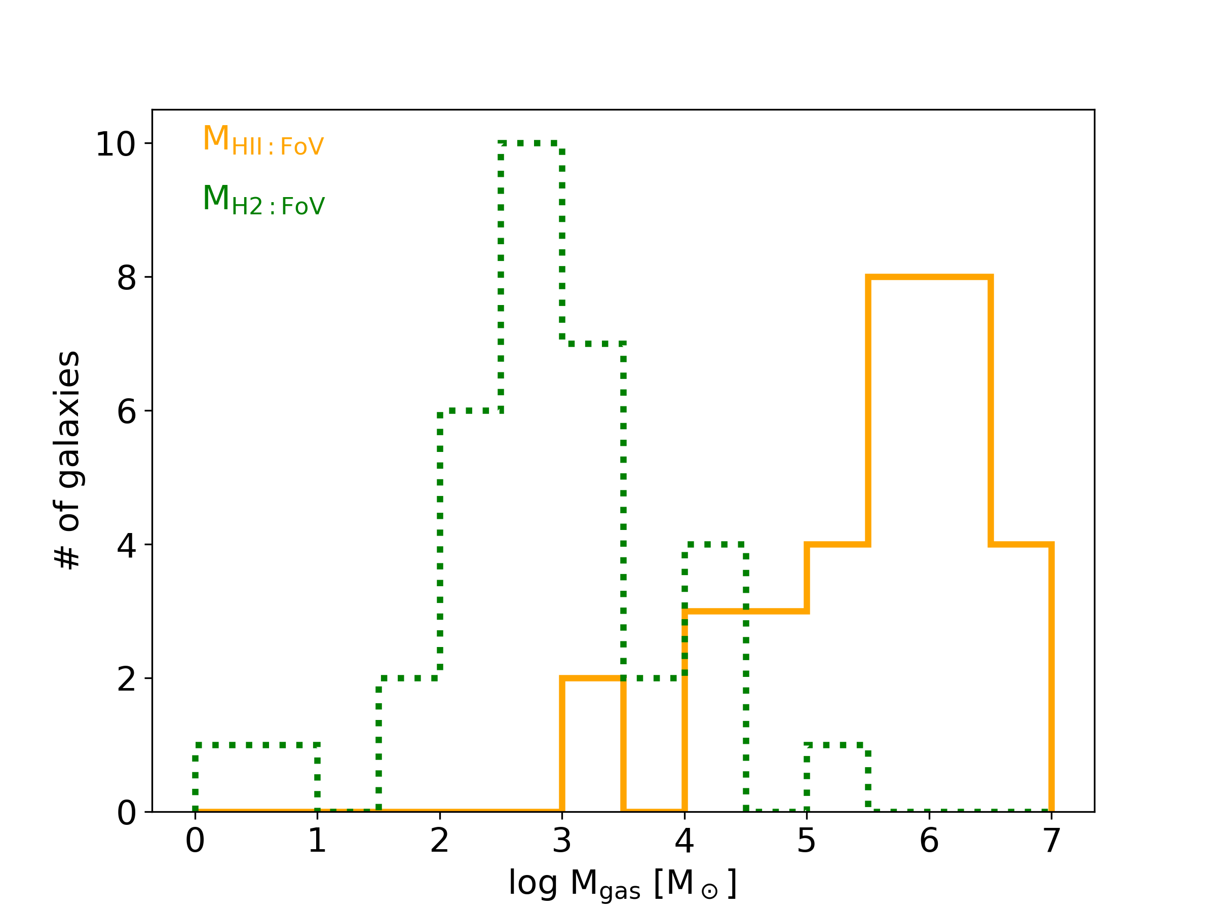
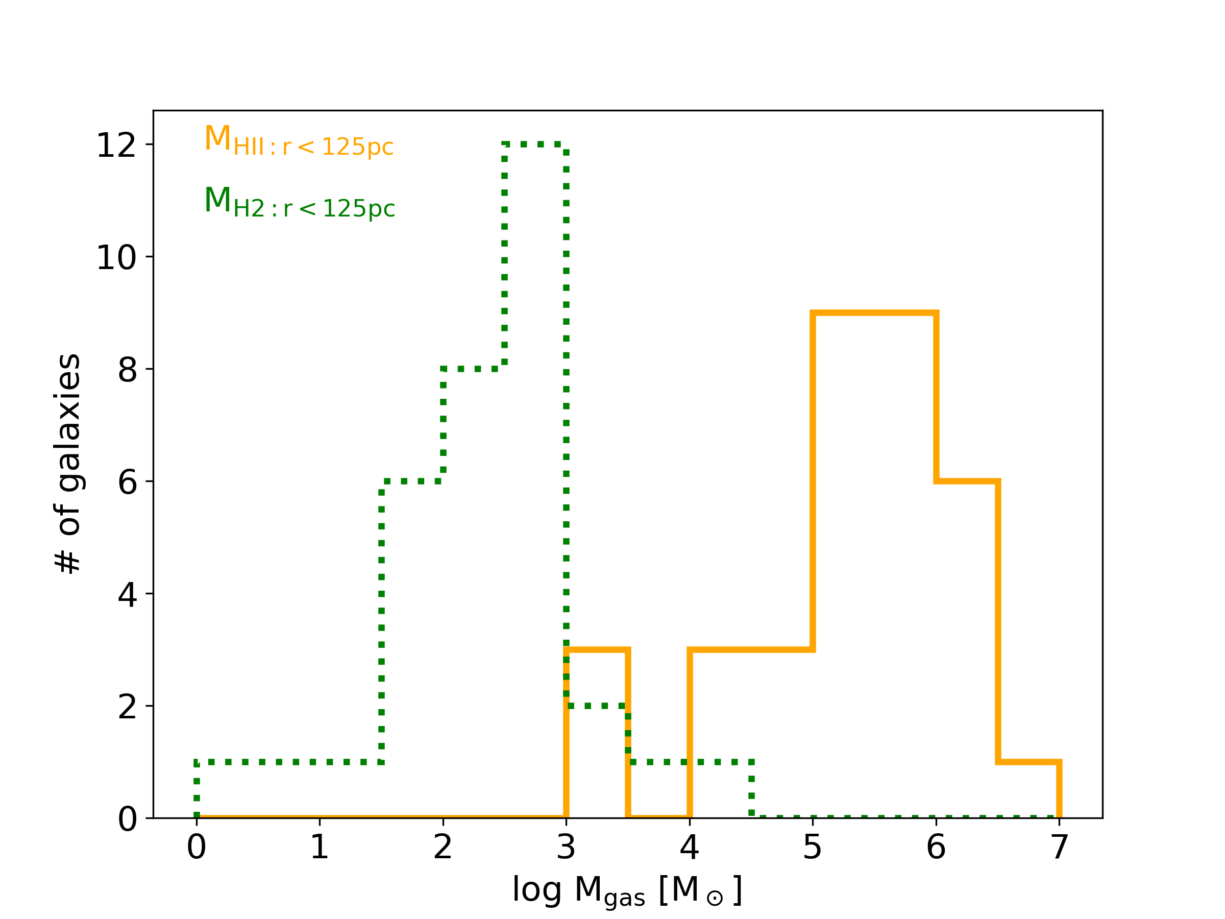
Figure 7: Molecular (green) and ionised (orange) hydrogen mass distributions for the galaxies of our sample, computed using the whole FoV (top) and the inner 125 pc radius (bottom).

3.4 H₂ vibrational and rotational temperatures

The H₂ 1–0 S(1)$\,2.1218\,\mu$m/2-1 S(1)$\,2.2477\,\mu$m and 1–0 S(2)$\,2.0338\,\mu$m/1–0 S(0)$\,2.2235\,\mu$m line ratios can be used to estimate the vibrational and rotational temperatures of H₂. Using $N_{i}/g_{i}=F_{i}\lambda_{i}/(A_{i}g_{i})={\rm exp}[-E_{i}/(k_{B}T_{\rm exc})]$, where $N_{i}$ are the column densities in the upper level, $g_{i}$ the statistical weights, $F_{i}$ and $\lambda_{i}$ are the line fluxes and wavelengths, $A_{i}$ are the transition probabilities, $E_{i}$ are the energies of the upper level, $T_{\rm exc}$ is the excitation temperature and $k_{B}$ is the Boltzmann constant. Using the transition probabilities from Turner et al. (1977), the rotational temperature is given by:

$$T_{\rm rot}\cong-{\frac{1113}{\ln\left(0.323\frac{F_{\rm H_{2}\,2.0338}}{F_{\rm H_{2}\,2.2235}}\right)}}$$ (3)

and the vibrational temperature by

$$T_{\rm vib}\cong{\frac{5594}{\ln\left(1.355\frac{F_{\rm H_{2}\,2.1218}}{F_{\rm H_{2}\,2.2477}}\right)}}.$$ (4)

We were able to estimate the H₂ vibrational temperature for 32 galaxies. For NGC 5548 and Mrk 1044 at least one of the H₂ emission lines used to determine $T_{\rm vib}$ is not detected in our NIFS data with an amplitude larger than twice the standard deviation of the adjacent continuum. We estimate the H₂ rotational temperature for 21 galaxies. 11 galaxies of our sample were observed using the K_long grating (Tab. 1), for which the spectral range does not include the H₂ 2.0338 $\mu$m emission line, needed to estimate the H₂ rotational temperature. In addition, this line is not detected for NGC 3516 and NGC 4235. In Figures 3 and 4 we show the maps of $T_{\rm rot}$ and $T_{\rm vib}$ for the type 2 and type 1 AGN and in Figure 5 we show the $T_{\rm vib}$ maps for the objects where the spectral range does not include the 1–0 S(2) line. Table 4 shows the median temperatures for each galaxy. The median values of the vibrational temperature are in the range from $\sim$2100 to $\sim$4300 K, while the rotational temperatures are in the range $\sim$450–1900 K. There is no difference between the mean temperatures in type 1 and type 2 AGN.

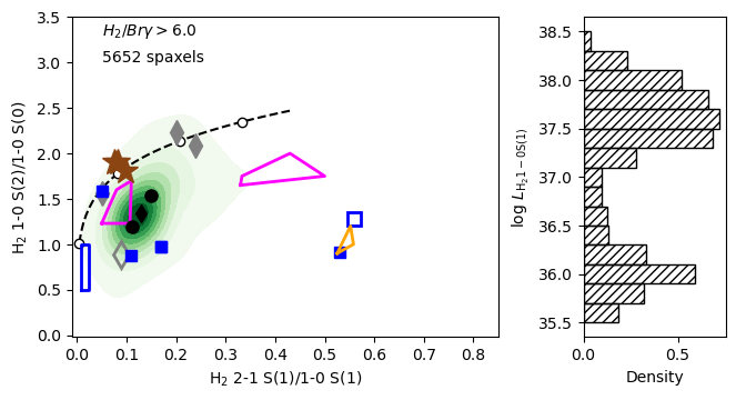
Figure 8: Density plots for the H₂ 2–1 S(1)/1–0 S(1) vs. 1–0 S(2)/1–0 S(0) diagnostic diagram for spaxels with H${}_{2}\,2.1218\,\mu$m/Br$\gamma>6.0$ (top left), $2.0<$H${}_{2}\,2.1218\,\mu$m/Br$\gamma<6.0$ (top right), $0.4<$H${}_{2}\,2.1218\,\mu$m/Br$\gamma<2.0$ (bottom left) and H${}_{2}\,2.1218\,\mu$m/Br$\gamma<0.4$ (botom right). Black circles in all diagrams correspond to the 25th percentile and 75th percentile of the observed line ratio. Black diamonds represent the median values.

The black dashed curve corresponds to the ratios for an isothermal and uniform density gas distribution for temperatures ranging from 1000 (left) to 4000 K (right) – the open circles identify the ratios in steps of 1000 K. The orange polygon represents the region occupied by the non-thermal UV excitation models of Black & van Dishoeck (1987) and the pink polygons cover the region of the photoionisation models of Dors et al. (2012). The blue rectangle covers the locus of the thermal UV excitation models of Sternberg & Dalgarno (1989), as computed by Mouri (1994) for gas densities ($n_{t}$) of 10⁵ and 10⁶ cm^-3 and UV scaling factors relative to the local interstellar radiation field $\chi$ from 10² to 10⁴. The filled blue squares are the UV thermal models from Davies et al. (2003) for $10^{3}<n_{t}<10^{6}$ cm^-3 and $10^{2}<\chi<10^{5}$, while the open blue square is from Sternberg & Dalgarno (1989) for $n_{t}=10^{3}$ cm^-3 and $\chi=10^{2}$. The brown stars are from the thermal X-ray models of Draine & Woods (1990), the gray open diamond is from the shock model of Kwan et al. (1977) and the gray filled diamonds represent the shock models from Smith (1995). The AGN photoionisation from Riffel et al. (2013a) span a wide range in both axes ($0\lesssim$H₂ 2–1 S(1)/1–0 S(1)$\lesssim 0.6$ and $0.5\lesssim$1–0 S(2)/1–0 S(0)$\lesssim 2.5$) and therefore is not shown in the figure. The right panels show the H${}_{2}\,2.1218\,\mu$m luminosity distributions for the spaxels used in the left panels, in logarithmic units of erg s^-1.

4 Discussion

4.1 Type 1 vs. type 2 AGN

According to the AGN Unification Model (Antonucci, 1993; Urry & Padovani, 1995), type 1 and type 2 AGN represent the same class of objects seen at distinct viewing angles. However, some recent results suggest these two classes may be intrinsically distinct objects (e.g., Elitzur, 2012; Elitzur et al., 2014; Villarroel & Korn, 2014; Prieto et al., 2014; Audibert et al., 2017), the tori of type 2 AGN having on average smaller opening angles and more clouds along the line of sight than for type 1 (Ramos Almeida et al., 2011).

Our sample presents the same number of type 1 and type 2 AGN and they follow similar luminosity and redshift distributions (Fig. 1), thus we can compare both AGN types in terms of the emission-line properties. We find the type 1 and type 2 AGN of our sample present similar H₂/Br$\gamma$ line ratios, ionised and hot molecular gas masses and H₂ excitation temperature distributions. They also present no difference in terms of the $\Delta$PA between the Br$\gamma$ and H₂ flux distributions and between the orientation of the major axis of the hosts and the emission-line flux distributions. These results support the unification scenario.

We find a statistically significant difference between type 1 and type 2 AGN only for the emission line equivalent widths at the nucleus (Fig. 6). Seyfert 1 nuclei show smaller equivalent widths than Seyfert 2 nuclei. The K-band continuum of AGN can present a strong contribution of hot dust emission from the inner border of the torus (e.g. Riffel et al., 2009c; Dumont et al., 2020). This component is present in about 90 per cent of Seyfert 1 nuclei, while only about 25 per cent of Seyfert 2 nuclei present this component (Riffel et al., 2009b). Thus, the smaller values of equivalent widths we observe in type 1 AGN may be due to stronger contributions of hot dust emission to the underlying continuum than those in type 2 AGN. Similar results are found for CO absorption-band heads at $\sim$2.3 $\mu$m, which can be diluted by the hot dust emission (Riffel et al., 2009b; Burtscher et al., 2015; Müller-Sánchez et al., 2018b). We find a decrease in the nuclear $EqW_{\rm Br\gamma}$ in 88% (15 objects) of Type 1 AGN, and in 47% (8 objects) of the type 2 AGN, as compared to the extra-nuclear $EqW_{\rm Br\gamma}$ values. The mean values of the ratio between the mean value of the nuclear $EqW_{\rm Br\gamma}$ (computed using an aperture with radius equal to the angular resolution of the data for each galaxy) and the mean extra-nuclear $EqW_{\rm Br\gamma}$ (computed using spaxels at distances larger than the angular resolution) is 1.35$\pm$0.27 and 0.58$\pm$0.14 for the type 2 and type 1 AGN in our sample, respectively. Considering only the galaxies that show a nuclear decrease in $EqW_{\rm Br\gamma}$, the mean ratios between the nuclear and extra-nuclear $EqW_{\rm Br\gamma}$ are 0.52$\pm$0.11 and 0.39$\pm$0.07 for type 2 and type 1 AGN, respectively.

The difference in the equivalent widths in type 1 and type 2 AGN can be reconciled with the AGN unification model, as in type 1 AGN we observe directly the contribution of the inner and hotter region of the dusty torus, while in type 2 AGN this structure is not visible in most objects. Smaller $EqW_{\rm Br\gamma}$ values at the nucleus compared to extra-nuclear regions could also be produced if the latter includes a larger contribution of young stellar populations than the former. Our results can be compared to those of Burtscher et al. (2015), who investigated the dilution of the K-band CO 2.3 $\mu$m absorption feature in a sample of nearby AGN hosts. They computed the intrinsic CO equivalent width (not affected by dilution) and found a wide range of values (from 6 to 14  Å), probably due to differences in the ages of the stellar populations in their sample. Our $EqW_{\rm Br\gamma}$ maps (Figs. 2,3,10 and 2) also show a wide range of values, which may be due to different stellar populations in the host galaxies. However, Burtscher et al. (2015) found no difference in the intrinsic CO equivalent widths of diluted and undiluted sources (see their Fig. 3), which provides a additional support that the nuclear decrease in $EqW_{\rm Br\gamma}$ in our sample is due to dilution of the line by the AGN continuum.

4.2 The origin of the H₂ emission

The origin of the H₂ near-IR emission lines in active galaxies has been investigated in several theoretical and observational studies (e.g Black & van Dishoeck, 1987; Hollenbach & McKee, 1989; Draine & Woods, 1990; Maloney et al., 1996; Rodríguez-Ardila et al., 2004; Rodríguez-Ardila et al., 2005; Lamperti et al., 2017), but it is still not clear which is the main excitation mechanism – if there is a dominant – of the H₂ molecule. In summary, three main processes can produce the H₂ emission: (i) fluorescent excitation by the absorption of soft-UV photons (912–1108 Å) in the Lyman and Werner bands (Black & van Dishoeck, 1987), (ii) excitation by shocks (Hollenbach & McKee, 1989) and (iii) excitation by X-ray illumination (Maloney et al., 1996). The first process is usually referred as non-thermal, while the latter two are commonly reported as thermal processes, where the H₂ emitting gas is in local thermodynamic equilibrium (LTE). In some cases, thermal and non-thermal processes are observed simultaneously with the H₂ 1–0 transitions in LTE, while the higher energy ones (H₂ 2–1 and H₂ 3–2) being due to fluorescent excitation of the dense gas (Davies et al., 2003, 2005).

In thermal processes, the rotational and vibrational temperatures are similar, as the gas is in LTE, while for fluorescent excitation the vibrational temperature is high ($T_{\rm vib}\sim$5000 K) and the rotational temperature is about a tenth of $T_{\rm vib}$, as the highest energy levels are overpopulated due to non-local UV photons compared to the prediction for a Maxwell-Boltzmann population (Sternberg & Dalgarno, 1989; Rodríguez-Ardila et al., 2004). As shown in Table 4, for all galaxies, but NGC 788, the median values of the rotational temperature are larger than 10 percent of the vibrational temperatures. On average, we find $\langle T_{\rm rot}/T_{\rm vib}\rangle=0.48\pm 0.31$. This value is consistent with measurements based on single aperture spectra of AGN (e.g. Rodríguez-Ardila et al., 2005; Riffel et al., 2013a).

The H₂/Br$\gamma$ line ratio is useful in the investigation of the origin of the H₂ emission. In star-forming regions and starburst galaxies, this ratio is usually smaller than 0.4, while AGN present $0.4<\rm H_{2}/Br\gamma<6.0$ and larger values are usually associated to shocks (Riffel et al., 2013a). We find the median values of H₂/Br$\gamma$ in our sample are within the range observed in AGN, but there is a trend of higher ratios being observed at larger distances from the nucleus for most galaxies, as seen in Tab. 3 and Figs. 2, 3, 10 and 2. Since the H₂ line intensity generally decreases with distance from the nucleus, an explanation for the higher values of the H₂/Br$\gamma$ away from the nucleus is that the Br$\gamma$ decreases faster with radius, i.e. it is enhanced very close around the AGN (excited primarily by the AGN) while the H₂ is excited by processes that operate on more extended spatial scales such as shocks.

In order to further investigate the H₂ emission origin, we construct the H₂ 2–1 S(1)/1–0 S(1) vs. 1–0 S(2)/1–0 S(0) diagnostic diagrams shown in Figure 8. The density plots show the observed line ratios for all spaxels where we were able to detect all H₂ emission lines. We separate the data into four diagrams, according to the H₂/Br$\gamma$ presented in the excitation maps (see Figs. 2, 3, 10, 2): H${}_{2}>6.0$ – indicative of shocks (top left panel), $2.0<\rm H_{2}/Br\gamma<6.0$ – high excitation AGN (top right panel), $0.4<\rm H_{2}/Br\gamma<2.0$ – low excitation AGN (bottom left panel) and H₂/Br$\gamma<0.4$ – typical value of starbursts (bottom right panel). The number of points in each plot is shown in the top-left corner of the corresponding panel.

The observed H₂ 2–1 S(1)/1–0 S(1) and 1–0 S(2)/1–0 S(0) line ratio distributions for H₂/Br$\gamma>0.4$ lie close to the region predicted by photoionisation (pink polygons) and shock models (gray symbols) suggesting thermal processes dominate the H₂ excitation. This result is in good agreement with previous works using single aperture measurements of the H₂ line fluxes (e.g. Rodríguez-Ardila et al., 2004; Rodríguez-Ardila et al., 2005; Riffel et al., 2013a). Here, we show not only the nuclear emission originates from thermal processes but that also the emission from locations furthest from the nucleus, as the vast majority (96 per cent) of the spaxels in our sample present H₂/Br$\gamma>$0.4.

Although the peak of the distributions of H₂ 2–1 S(1)/1–0 S(1) and 1–0 S(2)/1–0 S(0) is observed nearly at the same location for both spaxels with $0.4<\rm H_{2}/Br\gamma<2.0$, $2.0<\rm H_{2}/Br\gamma<6.0$ and H₂/Br$\gamma>6.0$, the distributions are distinct. For the $0.4<\rm H_{2}/Br\gamma<2.0$ (low excitation AGN) and $2.0<\rm H_{2}/Br\gamma<6.0$ (high excitation AGN) the luminosity distribution of the H₂2.1218$\mu$m is very similar and both H₂ 2–1 S(1)/1–0 S(1) and 1–0 S(2)/1–0 S(0) spread over a larger region in the diagnostic diagram. The peak in the diagnostic diagrams lie close to both the photoionisation model (pink polygons) and to the UV thermal models (filled blue squares) indicating that heating due to the AGN may be the cause of the gas excitation. Also, the fact that the points on the diagram are not distributed along the isothermal line indicates that the gas is not in LTE. For the typical AGN line ratio, $0.4<\rm H_{2}/Br\gamma<6.0$, the H₂ emission can either be produced by shocks (gray symbols) or by the AGN radiation field.

The H₂/Br$\gamma>6.0$ shows a more concentrated distribution in the diagnostic diagram and is particularly elongated towards higher values of 1–0 S(2)/1–0 S(0). The H₂2.1218$\mu$m distribution is concentrated towards higher values, indicating the higher ratios is due to the higher H₂ luminosity. This line ratio is more sensitive to shocks, as seen from the wider range of values predicted by distinct shock models for this ratio than for the 2–1 S(1)/1–0 S(1) (Kwan et al., 1977; Smith, 1995). Thus, the H₂ emission from locations with H₂/Br$\gamma>6.0$ likely originates from heating of the gas by shocks, as those produced by AGN winds (e.g. Riffel, 2020a).

For H₂/Br$\gamma<0.4$, typical of star-forming regions, the median values of 2–1 S(1)/1–0 S(1) and 1–0 S(2)/1–0 S(0) – 0.39 and 1.09, respectively – are close to the predicted values by the models of Black & van Dishoeck (1987) (orange polygon) for fluorescent excitation. The peak of the observed distribution of ratios is shifted to slightly lower values of 2–1 S(1)/1–0 S(1) than predicted by the models, but a large scatter is seen in both axes. This shift can be understood as a contamination of thermal excitation plus the dissociation of part of the H₂ molecules by the AGN radiation field, as seen in some objects (Storchi-Bergmann et al., 2009; Riffel et al., 2010a; Gnilka et al., 2020).

4.3 Mass reservoir in the central region and AGN feeding

The galaxies of our sample present masses of hot molecular gas ranging from a few tens of solar masses to 10⁴ M_⊙ and of ionised gas in the range $\sim 10^{3}-10^{7}$ M_⊙ within the inner 125 pc radius (Tab. 4). We can compare these masses with the mass accretion rate ($\dot{m}$) necessary to power the AGN, which is given by:

$$\dot{m}=\frac{L_{\rm bol}}{c^{2}\eta},$$ (5)

where $c$ is the light speed, $\eta$ is the efficiency of conversion of the rest mass energy of the accreted material into radiation assumed to be 0.1 (Frank et al., 2002) and $L_{\rm bol}$ is the AGN bolometric luminosity, which can be estimated from the hard X-ray (14-195 keV) luminosities ($L_{\rm X}$) listed in Tab. 1, by Ichikawa et al. (2017):

$$\log{L_{\rm bol}}=0.0378(\log{L_{\rm X}})^{2}-2.03\log{L_{\rm X}}+61.6.$$ (6)

Figure 9 shows the feeding time ($t_{f}={M_{\rm gas}/\dot{m}}$) distributions for the galaxies computed using the hot molecular and ionised gas masses calculated in the previous sections within the inner 125 pc. We find the mass of ionised gas alone can feed the central AGN for 10⁵–10⁸ yr at the current accretion rates. The mass of hot molecular gas is on average 3 orders of magnitude smaller than that of ionised gas. We emphasize that the feeding times estimated above should be treated as an upper limit, as they are based on the total line fluxes and we do not separate the components associated to non-circular motions (e.g. due to inflows and outflows).

The hot molecular and ionised gas masses represent only the “tip of the iceberg” of the the total gas mass in the center of galaxies. Dempsey & Zakamska (2018) find the mass of the NLR, measured from emission-line fluxes of the ionised gas, is underestimated because the gas behind the ionisation front is invisible in ionised transitions. This gas may be in the molecular phase, dominated by cold molecular gas, and we now know that the mass of cold molecular gas correlates with the H₂ 2.1218 $\mu$m luminosity – and thus with the hot H₂ mass (Dale et al., 2005; Müller Sánchez et al., 2006; Mazzalay et al., 2013). These studies found that the amount of cold molecular gas is 10⁵–10⁸ times that of hot H₂. Thus, the cold molecular gas could provide fuel necessary to power the AGN for an activity cycle of 10⁵ to 10⁶ yr (e.g. Novak et al., 2011) and still remain available to form new stars in the nuclear region.

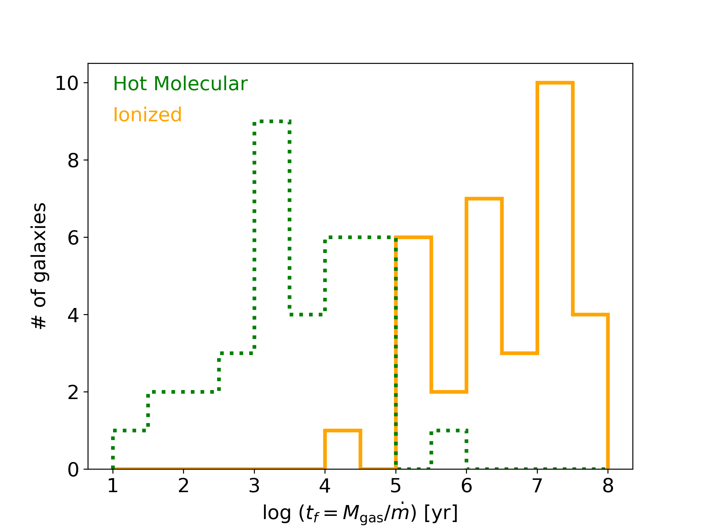
Figure 9: Distribution of the AGN feeding time with the available masses of hot molecular (green) and ionised (orange) hydrogen mass in the inner 125 pc radius.

5 Conclusions

We have used Gemini NIFS K-band observations to map the H₂ and Br$\gamma$ emission distribution within the inner 0.04–2 kpc of a sample of 36 active galaxies with $0.001\lesssim z\lesssim 0.056$ and hard X-ray luminosities in the range $41\lesssim\log L_{\rm X}/({\rm erg\,s^{-1}})\lesssim 45$. The spatial resolutions at the galaxies range from 6 to 250 pc and the field of view covers from the inner 75$\times$75 pc² to 3.6$\times$3.6 kpc². The main conclusions of this work are:

• Extended H${}_{2}\,2.1218\,\mu$m and Br$\gamma$ emission is observed in 34/36 galaxies of our sample. There is no statistically significant difference between the orientation of the H₂ and Br$\gamma$ flux distributions relative to the orientation of the major axis of the host galaxy ($\Delta$PA). We find $\Delta$PA larger than 30^∘ in 15 galaxies (42 %) for the Br$\gamma$ and in 16 galaxies (44 %) for H₂.

• The H₂ emission is usually more spread over the field of view, while the Br$\gamma$ shows a more collimated flux distribution in most cases and a steeper flux gradient, decreasing with the distance from the nucleus. We find offsets larger than 30^∘ between the orientations of the H${}_{2}\,$2.1218$\mu$m and Br$\gamma$ flux distributions in 45 % of our sample. On average, the radius that contains 50 per cent of the total H₂ emission is $\sim$60 per cent larger than that for Br$\gamma$.

• We derive the H₂ rotational and vibrational temperatures based on the observed H₂ 1-0 S(1)$\,2.1218\,\mu$m/2-1 S(1)$\,2.2477\,\mu$m and 1-0 S(2)$\,2.0338\,\mu$m/1-0S(0)$\,2.2235\,\mu$m line ratios. The median values are in the ranges 2100–4300 K and 450–1900 K for the vibrational and rotational temperatures, respectively, with the mean ratio between the two of 0.43$\pm$0.15, indicating dominant thermal excitation for the gas.

• Type 1 and type 2 AGN show similar emission-line flux distributions, ratios, H₂ excitation temperatures and gas masses, supporting the AGN unification scenario.

• Type 1 and 2 AGN differ only in their nuclear Br$\gamma$ equivalent widths, which are smaller in type 1 AGN due to larger contributions of hot dust emission to the K-band continuum in type 1 nuclei.

• The distribution of points in the H₂ 2–1 S(1)/1–0 S(1) vs. 1–0 S(2)/1–0 S(0) diagram in regions with H₂/Br$\gamma>0.4$ (96 % of all spaxels with flux measurements) are consistent with predictions of photoionisation and shock models, confirming that the main excitation mechanism of the H₂ molecule are thermal processes, not only at the nucleus but also in the extranuclear regions.

• The gas thermal excitation usually increases outwards with H₂/Br$\gamma$ values increasing from $<2$ in the nucleus to values up to 6 outwards.

• In locations with H₂/Br$\gamma>$6.0, the most likely H₂ excitation mechanism are shocks, as indicated by the H₂ 2–1 S(1)/1–0 S(1) and 1–0 S(2)/1–0 S(0) line ratios. This is observed mostly in locations away from the nucleus, for $\sim$40 per cent of the galaxies.

• Most of the regions with H₂/Br$\gamma<0.4$ (4 % of the spaxels with flux measurements) are consistent with fluorescent excitation of the H₂, but dissociation of the H₂ molecule by the AGN radiation cannot be ruled out in galaxies with small H₂/Br$\gamma$ nuclear values. This is observed in $\sim$25 per cent of the sample.

• The mass of hot molecular and ionised gas in the inner 125 pc radius are in the ranges $10^{1}-10^{4}$ M_⊙ and $10^{4}-10^{6}$ M_⊙, respectively. The masses computed for the whole NIFS field of view are about one order of magnitude larger.

• The mass of ionised gas within the inner 125 pc radius alone is more than enough to power the AGN in our sample for a duty cycle of $10^{6}$ yr at their current accretion rates.

Data availability

Most of the data used in this paper is available in the Gemini Science Archive at https://archive.gemini.edu/searchform with the project codes listed in Table 1. Processed datacubes used will be shared on reasonable request to the corresponding author.

Appendix A Gemini NIFS measurements

For all galaxies, north is up and east is to the left.

References

- Antonucci (1993) Antonucci R., 1993, ARA&A, 31, 473
- Audibert et al. (2017) Audibert A., Riffel R., Sales D. A., Pastoriza M. G., Ruschel-Dutra D., 2017, MNRAS, 464, 2139
- Barbosa et al. (2014) Barbosa F. K. B., Storchi-Bergmann T., McGregor P., Vale T. B., Rogemar Riffel A., 2014, MNRAS, 445, 2353
- Baron & Netzer (2019) Baron D., Netzer H., 2019, MNRAS, 486, 4290
- Barth et al. (1999) Barth A. J., Filippenko A. V., Moran E. C., 1999, ApJ, 515, L61
- Black & van Dishoeck (1987) Black J. H., van Dishoeck E. F., 1987, ApJ, 322, 412
- Brum et al. (2017) Brum C., Riffel R. A., Storchi-Bergmann T., Robinson A., Schnorr Müller A., Lena D., 2017, MNRAS, 469, 3405
- Brum et al. (2019) Brum C., et al., 2019, MNRAS, 486, 691
- Burtscher et al. (2015) Burtscher L., et al., 2015, A&A, 578, A47
- Caglar et al. (2020) Caglar T., et al., 2020, A&A, 634, A114
- Colina et al. (2015) Colina L., et al., 2015, A&A, 578, A48
- Daddi et al. (2010) Daddi E., et al., 2010, ApJ, 713, 686
- Dahmer-Hahn et al. (2019a) Dahmer-Hahn L. G., et al., 2019a, MNRAS, 482, 5211
- Dahmer-Hahn et al. (2019b) Dahmer-Hahn L. G., et al., 2019b, MNRAS, 489, 5653
- Dale et al. (2005) Dale D. A., Sheth K., Helou G., Regan M. W., Hüttemeister S., 2005, AJ, 129, 2197
- Davies et al. (2003) Davies R. I., Sternberg A., Lehnert M., Tacconi-Garman L. E., 2003, ApJ, 597, 907
- Davies et al. (2005) Davies R. I., Sternberg A., Lehnert M. D., Tacconi-Garman L. E., 2005, ApJ, 633, 105
- Davies et al. (2009) Davies R. I., Maciejewski W., Hicks E. K. S., Tacconi L. J., Genzel R., Engel H., 2009, ApJ, 702, 114
- Davies et al. (2014) Davies R. I., et al., 2014, ApJ, 792, 101
- Davies et al. (2015) Davies R. I., et al., 2015, ApJ, 806, 127
- Davies et al. (2020) Davies R., et al., 2020, MNRAS,
- Dempsey & Zakamska (2018) Dempsey R., Zakamska N. L., 2018, MNRAS, 477, 4615
- Diniz et al. (2015) Diniz M. R., Riffel R. A., Storchi-Bergmann T., Winge C., 2015, MNRAS, 453, 1727
- Diniz et al. (2018) Diniz M. R., Riffel R. A., Dors O. L., 2018, Research Notes of the American Astronomical Society, 2, 3
- Dors et al. (2008) Dors O. L. J., Storchi-Bergmann T., Riffel R. A., Schimdt A. A., 2008, A&A, 482, 59
- Dors et al. (2012) Dors Oli L. J., Riffel R. A., Cardaci M. V., Hägele G. F., Krabbe Á. C., Pérez-Montero E., Rodrigues I., 2012, MNRAS, 422, 252
- Dors et al. (2014) Dors O. L., Cardaci M. V., Hägele G. F., Krabbe Â. C., 2014, MNRAS, 443, 1291
- Dors et al. (2020) Dors O. L., Maiolino R., Cardaci M. V., Hägele G. F., Krabbe A. C., Pérez-Montero E., Armah M., 2020, MNRAS,
- Draine & Woods (1990) Draine B. T., Woods D. T., 1990, ApJ, 363, 464
- Drehmer et al. (2015) Drehmer D. A., Storchi-Bergmann T., Ferrari F., Cappellari M., Riffel R. A., 2015, MNRAS, 450, 128
- Dumont et al. (2020) Dumont A., Seth A. C., Strader J., Greene J. E., Burtscher L., Neumayer N., 2020, ApJ, 888, 19
- Durré & Mould (2014) Durré M., Mould J., 2014, ApJ, 784, 79
- Durré & Mould (2018) Durré M., Mould J., 2018, ApJ, 867, 149
- Elitzur (2012) Elitzur M., 2012, ApJ, 747, L33
- Elitzur et al. (2014) Elitzur M., Ho L. C., Trump J. R., 2014, MNRAS, 438, 3340
- Fazeli et al. (2020) Fazeli N., Eckart A., Busch G., Yttergren M., Combes F., Misquitta P., Straubmeier C., 2020, A&A, 638, A36
- Fischer et al. (2017) Fischer T. C., et al., 2017, ApJ, 834, 30
- Frank et al. (2002) Frank J., King A., Raine D. J., 2002, Accretion Power in Astrophysics: Third Edition
- Freitas et al. (2018) Freitas I. C., et al., 2018, MNRAS, 476, 2760
- Genzel et al. (2010) Genzel R., et al., 2010, MNRAS, 407, 2091
- Gnilka et al. (2020) Gnilka C. L., et al., 2020, ApJ, 893, 80
- Gonzalez Delgado & Perez (1997) Gonzalez Delgado R. M., Perez E., 1997, MNRAS, 284, 931
- Harrison (2017) Harrison C. M., 2017, Nature Astronomy, 1, 0165
- Harrison et al. (2018) Harrison C. M., Costa T., Tadhunter C. N., Flütsch A., Kakkad D., Perna M., Vietri G., 2018, Nature Astronomy, 2, 198
- Heckman (1980) Heckman T. M., 1980, A&A, 500, 187
- Heckman & Best (2014) Heckman T. M., Best P. N., 2014, ARA&A, 52, 589
- Hicks et al. (2009) Hicks E. K. S., Davies R. I., Malkan M. A., Genzel R., Tacconi L. J., Müller Sánchez F., Sternberg A., 2009, ApJ, 696, 448
- Ho et al. (1997) Ho L. C., Filippenko A. V., Sargent W. L. W., Peng C. Y., 1997, ApJS, 112, 391
- Hollenbach & McKee (1989) Hollenbach D., McKee C. F., 1989, ApJ, 342, 306
- Hopkins & Quataert (2010) Hopkins P. F., Quataert E., 2010, MNRAS, 407, 1529
- Husemann et al. (2019) Husemann B., et al., 2019, A&A, 627, A53
- Ichikawa et al. (2017) Ichikawa K., Ricci C., Ueda Y., Matsuoka K., Toba Y., Kawamuro T., Trakhtenbrot B., Koss M. J., 2017, ApJ, 835, 74
- Ilha et al. (2016) Ilha G. d. S., Bianchin M., Riffel R. A., 2016, Ap&SS, 361, 178
- Jin et al. (2016) Jin Y., et al., 2016, MNRAS, 463, 913
- Kakkad et al. (2018) Kakkad D., et al., 2018, A&A, 618, A6
- Keel (1990) Keel W. C., 1990, AJ, 100, 356
- Kormendy & Ho (2013) Kormendy J., Ho L. C., 2013, ARA&A, 51, 511
- Kwan et al. (1977) Kwan J. H., Gatley I., Merrill K. M., Probst R., Weintraub D. A., 1977, ApJ, 216, 713
- Lamperti et al. (2017) Lamperti I., et al., 2017, MNRAS, 467, 540
- Lin et al. (2018) Lin M.-Y., et al., 2018, MNRAS, 473, 4582
- Liu et al. (2013) Liu G., Zakamska N. L., Greene J. E., Nesvadba N. P. H., Liu X., 2013, MNRAS, 436, 2576
- Lutz et al. (2003) Lutz D., Sturm E., Genzel R., Spoon H. W. W., Moorwood A. F. M., Netzer H., Sternberg A., 2003, A&A, 409, 867
- Maloney et al. (1996) Maloney P. R., Hollenbach D. J., Tielens A. G. G. M., 1996, ApJ, 466, 561
- May & Steiner (2017) May D., Steiner J. E., 2017, MNRAS, 469, 994
- May et al. (2020) May D., Steiner J. E., Menezes R. B., Williams D. R. A., Wang J., 2020, MNRAS, 496, 1488
- Mazzalay et al. (2013) Mazzalay X., et al., 2013, MNRAS, 428, 2389
- McGregor et al. (2003) McGregor P. J., et al., 2003, Gemini near-infrared integral field spectrograph (NIFS). Proceedings of the SPIE, pp 1581–1591, doi:10.1117/12.459448
- Mouri (1994) Mouri H., 1994, ApJ, 427, 777
- Müller Sánchez et al. (2006) Müller Sánchez F., Davies R. I., Eisenhauer F., Tacconi L. J., Genzel R., Sternberg A., 2006, A&A, 454, 481
- Müller-Sánchez et al. (2018a) Müller-Sánchez F., Nevin R., Comerford J. M., Davies R. I., Privon G. C., Treister E., 2018a, Nature, 556, 345
- Müller-Sánchez et al. (2018b) Müller-Sánchez F., Hicks E. K. S., Malkan M., Davies R., Yu P. C., Shaver S., Davis B., 2018b, ApJ, 858, 48
- Novak et al. (2011) Novak G. S., Ostriker J. P., Ciotti L., 2011, ApJ, 737, 26
- Oh et al. (2018) Oh K., et al., 2018, ApJS, 235, 4
- Osterbrock & Ferland (2006) Osterbrock D. E., Ferland G. J., 2006, Astrophysics of gaseous nebulae and active galactic nuclei. University Science Books
- Pasquali et al. (2004) Pasquali A., Gallagher J. S., de Grijs R., 2004, A&A, 415, 103
- Paturel et al. (2003) Paturel G., Petit C., Prugniel P., Theureau G., Rousseau J., Brouty M., Dubois P., Cambrésy L., 2003, A&A, 412, 45
- Prieto et al. (2014) Prieto M. A., Mezcua M., Fernández-Ontiveros J. A., Schartmann M., 2014, MNRAS, 442, 2145
- Puxley et al. (1990) Puxley P. J., Hawarden T. G., Mountain C. M., 1990, ApJ, 364, 77
- Ramos Almeida et al. (2011) Ramos Almeida C., et al., 2011, ApJ, 731, 92
- Reunanen et al. (2002) Reunanen J., Kotilainen J. K., Prieto M. A., 2002, MNRAS, 331, 154
- Ricci et al. (2014) Ricci T. V., Steiner J. E., Menezes R. B., 2014, MNRAS, 440, 2419
- Riffel (2020a) Riffel R. A., 2020a, MNRAS, 494, 2004
- Riffel (2020b) Riffel R. A., 2020b, MNRAS, 494, 2004
- Riffel et al. (2006) Riffel R., Rodríguez-Ardila A., Pastoriza M. G., 2006, A&A, 457, 61
- Riffel et al. (2008) Riffel R. A., Storchi-Bergmann T., Winge C., McGregor P. J., Beck T., Schmitt H., 2008, MNRAS, 385, 1129
- Riffel et al. (2009a) Riffel R. A., Storchi-Bergmann T., Dors O. L., Winge C., 2009a, MNRAS, 393, 783
- Riffel et al. (2009b) Riffel R., Pastoriza M. G., Rodríguez-Ardila A., Bonatto C., 2009b, MNRAS, 400, 273
- Riffel et al. (2009c) Riffel R. A., Storchi-Bergmann T., McGregor P. J., 2009c, ApJ, 698, 1767
- Riffel et al. (2010a) Riffel R. A., Storchi-Bergmann T., Nagar N. M., 2010a, MNRAS, 404, 166
- Riffel et al. (2010b) Riffel R. A., Storchi-Bergmann T., Riffel R., Pastoriza M. G., 2010b, ApJ, 713, 469
- Riffel et al. (2013a) Riffel R., Rodríguez-Ardila A., Aleman I., Brotherton M. S., Pastoriza M. G., Bonatto C., Dors O. L., 2013a, MNRAS, 430, 2002
- Riffel et al. (2013b) Riffel R. A., Storchi-Bergmann T., Winge C., 2013b, MNRAS, 430, 2249
- Riffel et al. (2014) Riffel R. A., Vale T. B., Storchi-Bergmann T., McGregor P. J., 2014, MNRAS, 442, 656
- Riffel et al. (2017) Riffel R. A., Storchi-Bergmann T., Riffel R., Dahmer-Hahn L. G., Diniz M. R., Schönell A. J., Dametto N. Z., 2017, MNRAS, 470, 992
- Riffel et al. (2018) Riffel R. A., et al., 2018, MNRAS, 474, 1373
- Riffel et al. (2020) Riffel R. A., Storchi-Bergmann T., Zakamska N. L., Riffel R., 2020, MNRAS, 496, 4857
- Riffel et al. (2021) Riffel R. A., Bianchin M., Riffel R., Storchi-Bergmann T., Schönell A. J., Dahmer-Hahn L. G., Dametto N. Z., Diniz M. R., 2021, MNRAS,
- Rodríguez-Ardila et al. (2004) Rodríguez-Ardila A., Pastoriza M. G., Viegas S., Sigut T. A. A., Pradhan A. K., 2004, A&A, 425, 457
- Rodríguez-Ardila et al. (2005) Rodríguez-Ardila A., Riffel R., Pastoriza M. G., 2005, MNRAS, 364, 1041
- Rosario et al. (2019) Rosario D. J., Togi A., Burtscher L., Davies R. I., Shimizu T. T., Lutz D., 2019, ApJ, 875, L8
- Ruschel-Dutra (2020) Ruschel-Dutra D., 2020, danielrd6/ifscube v1.0, doi:10.5281/zenodo.3945237, https://doi.org/10.5281/zenodo.3945237
- Sargent et al. (2014) Sargent M. T., et al., 2014, ApJ, 793, 19
- Scharwächter et al. (2013) Scharwächter J., McGregor P. J., Dopita M. A., Beck T. L., 2013, MNRAS, 429, 2315
- Schinnerer et al. (2000) Schinnerer E., Eckart A., Tacconi L. J., 2000, ApJ, 533, 826
- Schönell et al. (2014) Schönell A. J., Riffel R. A., Storchi-Bergmann T., Winge C., 2014, MNRAS, 445, 414
- Schönell et al. (2017) Schönell Astor J. J., Storchi-Bergmann T., Riffel R. A., Riffel R., 2017, MNRAS, 464, 1771
- Schönell et al. (2019) Schönell A. J., Storchi-Bergmann T., Riffel R. A., Riffel R., Bianchin M., Dahmer-Hahn L. G., Diniz M. R., Dametto N. Z., 2019, MNRAS, 485, 2054
- Scoville et al. (1982) Scoville N. Z., Hall D. N. B., Ridgway S. T., Kleinmann S. G., 1982, ApJ, 253, 136
- Shimizu et al. (2019) Shimizu T. T., et al., 2019, MNRAS, 490, 5860
- Silverman et al. (2015) Silverman J. D., et al., 2015, ApJ, 812, L23
- Smith (1995) Smith M. D., 1995, A&A, 296, 789
- Sternberg & Dalgarno (1989) Sternberg A., Dalgarno A., 1989, ApJ, 338, 197
- Storchi-Bergmann & Schnorr-Müller (2019) Storchi-Bergmann T., Schnorr-Müller A., 2019, Nature Astronomy, 3, 48
- Storchi-Bergmann et al. (2009) Storchi-Bergmann T., McGregor P. J., Riffel R. A., Simões Lopes R., Beck T., Dopita M., 2009, MNRAS, 394, 1148
- Turner et al. (1977) Turner J., Kirby-Docken K., Dalgarno A., 1977, ApJS, 35, 281
- Urry & Padovani (1995) Urry C. M., Padovani P., 1995, PASP, 107, 803
- Villarroel & Korn (2014) Villarroel B., Korn A. J., 2014, Nature Physics, 10, 417
- Wilgenbus et al. (2000) Wilgenbus D., Cabrit S., Pineau des Forêts G., Flower D. R., 2000, A&A, 356, 1010
- de Vaucouleurs et al. (1991) de Vaucouleurs G., de Vaucouleurs A., Corwin Herold G. J., Buta R. J., Paturel G., Fouque P., 1991, Third Reference Catalogue of Bright Galaxies