Initial Perturbation of the Mean Curvature Flow for closed limit shrinker

Abstract.

This is a contribution to the program of dynamical approach to mean curvature flow initiated by Colding and Minicozzi. In this paper, we prove two main theorems. The first one is local in nature and the second one is global. In this first result, we pursue the stream of ideas of [CM3] and get a slight refinement of their results. We apply the invariant manifold theory from hyperbolic dynamics to study the dynamics close to a closed shrinker that is not a sphere. In the second theorem, we show that if a hypersurface under the rescaled mean curvature flow converges to a closed shrinker that is not a sphere, then a generic perturbation on initial data would make the flow leave a small neighborhood of the shrinker and never come back. The key is to prove that a positive perturbation would drift to the first eigenfunction direction under the linearized equation. This result can be viewed as a global unstable manifold theorem in the most unstable direction.

1. Introduction

A family of hypersurfaces $\{\mathbf{M}_{t}\}\subset\mathbb{R}^{n+1}$ is flow by mean curvature if they satisfy the equation

$$\partial_{t}x=-H\mathbf{n}.$$

Here $x$ is the position vector of $\mathbf{M}_{t}$, $H$ is the mean curvature of $\mathbf{M}_{t}$ and $\mathbf{n}$ is the outer unit normal vector field on $\mathbf{M}_{t}$.

Mean curvature flow (MCF) of closed hypersurfaces must generate finite time singularities, and the singularities are modeled by the tangent flow, see [H], [Wh1], [I]. The tangent flow at the singular space-time point can be characterized by the rescaled mean curvature flow (RMCF), which is a family of hypersurfaces $M_{t}$ satisfying the equation

$$\partial_{t}x=-\left(H-\frac{\langle x,\mathbf{n}\rangle}{2}\right)\mathbf{n}.$$

In particular, self-shrinkers, which are hypersurfaces satisfying the equation $H=\frac{\langle x,\mathbf{n}\rangle}{2}$ are static under RMCF. MCF and RMCF are equivalent to each other up to a space-time rescaling. In this paper, we only consider MCF and RMCF which are closed embedded hypersurfaces.

In this paper, we investigate the behaviour of MCF near a singularity modeled by a closed self-shrinker using a dynamical point of view. Our main results focus on two aspects: one is a local result, which focuses on the local behaviour of MCF near a singularity modeled by a closed self-shrinker; the other is a global result, which focuses on the behaviour of MCF near a singularity modeled by a closed self-shrinker after an initial positive perturbation.

Our first theorem generalizes a result of Colding-Minicozzi [CM3]. We give a characterization of local dynamics near a closed embedded self-shrinker. In Section 2, we shall introduce a Banach space $\mathcal{X}$ that is a refinement of $C^{2,\alpha}(\Sigma)$, so that $0\in\mathcal{X}$ corresponds to $\Sigma$ and we write a smooth $n$-manifold sufficiently close to $\Sigma$ in the $\mathcal{X}$-norm as a point in $\mathcal{X}$ close to zero. Roughly speaking, we prove the following theorem:

Theorem 1.1 (Theorem 2.1).

Let $\Sigma^{n}$ be an $n$-dimensional closed smooth embedded self-shrinker in $\mathbb{R}^{n+1}$. Then there exist local Lipschitz stable/unstable/center/center-unstable manifolds in a neighborhood of $0\in\mathcal{X}$ under the dynamics of truncated RMCF.

The precise statement of this theorem is quite technical, and we leave it to Section 2. Moreover, we obtain a number of properties of these stable/unstable/center/center-unstable manifolds.

The existence of invariant manifolds is crucial in the study of the dynamical stability of an evolutionary equation near a fixed point. This result gives a rather clear picture of the dynamics in a small neighborhood of the shrinker. For instance, for any orbit with an initial condition on the stable manifold, its forward orbit approaches $\Sigma$ exponentially under the RMCF, while for any orbit with an initial condition on the unstable manifold, its backward orbit approaches $\Sigma$ exponentially under the RMCF. The latter gives ancient solutions which were constructed in [ChM, CCMS1]. For a generic initial point, its orbit is shadowed by an orbit on the center-unstable manifold, which has a finite dimension.

There are various notions of stability near a self-shrinker. The $F$-stability and entropy stability introduced by Colding and Minicozzi in [CM1] are based on the variations of the $F$-functional (also known as Gaussian area) of a hypersurface $M$, defined by

$$F(M)=\int_{M}e^{-\frac{|x|^{2}}{4}}d\mu$$

and the entropy defined as the supremum of the $F$-functional of $M$ under all possible dilations and translations. i.e.

$$\lambda(M)=\sup_{x\in\mathbb{R}^{n+1},t\in(0,\infty)}F(t^{-1}(M-x)).$$

If we are interested in the dynamics of the RMCF in a neighborhood of the shrinker, we may use the following notion of dynamical stability. We say that $\Sigma$ is dynamically stable, if for every small neighborhood $U$ of zero in $\mathcal{X}$ there exists a small neighborhood $V$, such that every initial datum that are chosen in $U$ have forward orbits always staying in $V$. If $\Sigma$ is a compact self-shrinker but not a sphere, then no matter how small $U$ is, we can always choose an initial condition on the unstable manifold modulo the rigid transformation of $\Sigma$, such that its forward orbit escapes any small open set $V$. The dynamical instability for compact shrinkers agrees with $F$-instability and entropy instability defined by Colding and Minicozzi.

The problem is essentially reduced to constructing invariant manifolds for a nonlinear parabolic equation of the form $\partial_{t}u=L_{\Sigma}u+f(x,u,\nabla u,\nabla^{2}u)$, where $f=\mathcal{M}u-L_{\Sigma}u$ (c.f. Lemma A.3 for the notations). We may write the solution to the equation in terms of the DuHamel principle. However, the presence of $\nabla^{2}u$ in the nonlinear term $f$ makes the solution not $C^{1}$ in $t$. The way to overcome this difficulty is to invoke the theory of maximal regularity. We will discuss how this works in Section 3.2.

Next, we move from local dynamics to global dynamics. We remark that this second part on the global dynamics is totally independent of the first part on the invariant manifolds.

In [CM1], Colding-Minicozzi used $F$-stability to characterize the genericity of self-shrinkers. In particular, they proved that the sphere with radius $\sqrt{2n}$ is the only generic closed self-shrinker of mean curvature flow. We prove that we can avoid those non-generic closed singularities by perturbing the initial data.

Theorem 1.2.

Let $\{M_{t}\}_{t\in[0,\infty)}$ be a RMCF with $M_{t}\to\Sigma$ smoothly as $t\to\infty$ where $\Sigma$ is a compact shrinker that is not a sphere. Then there exists an open dense subset $\mathcal{S}$ of $\{v_{0}\in C^{2,\alpha}(M_{0})\ |\ \|v_{0}\|=1\}$, such that for any $v_{0}\in\mathcal{S}$, there exist $\varepsilon_{0}>0$ such that for all $0<\varepsilon<\varepsilon_{0}$, there exists $T>0$ such that for the perturbed flow $\{\widetilde{M}_{t}\}$ starting from $\{x+\varepsilon v_{0}(x)\mathbf{n}(x)\ |\ x\in M_{0}\}$, we have $\lambda(\widetilde{M}_{T})<\lambda(\Sigma).$

Here we emphasize that the initial perturbations are not necessarily positive. In [CCMS1], the authors studied initial perturbation using techniques from geometric measure theory, with a different notion of genericity. In the following, we use the word “generic” in the sense of Theorem 1.2. The equivalence of RMCF and MCF gives the following corollary.

Corollary 1.3.

Suppose $\{\mathbf{M}_{t}\}_{t\in[0,T)}$ is a MCF and the first time singularity is characterized by a multiplicity $1$ closed self-shrinker $\Sigma$ which is not a sphere. Then we can perturb $\mathbf{M}_{0}$ generically to a nearby hypersurface $\widetilde{\mathbf{M}}_{0}$ such that the MCF $\{\widetilde{\mathbf{M}}_{t}\}$ starting from $\widetilde{\mathbf{M}}_{0}$ will never encounter a singularity characterized by $\Sigma$.

This result is an attempt to solve Conjecture 8.2 in [CMP]. In [CMP], Colding-Minicozzi-Pedersen proposed that after a generic perturbation on the initial data of a MCF, the perturbed MCF will only encounter generic singularities. A consequence of our Corollary 1.3 is that, in $\mathbb{R}^{3}$, after a perturbation on the initial data, the perturbed MCF will encounter the first singularity either non-compact, or has higher multiplicity, or a sphere.

Corollary 1.4.

Consider MCF in $\mathbb{R}^{3}$. After a generic small perturbation on initial data, the first singularity of a MCF is modeled by either a sphere, or a non-compact self-shrinker, or a higher multiplicity self-shrinker.

The results are of some interest for the following reason. Consider the following finite dimensional dynamical system in $\mathbb{R}^{n}$ given by $x^{\prime}=F(x)$ with a fixed point $0$. Suppose for simplicity that $DF(0)$ is symmetric and has only negative and positive eigenvalues. We can construct local invariant manifolds for the nonlinear system in a small neighborhood of zero. Moreover, we can also construct global stable and unstable manifolds. The global stable manifold is constructed by taking the union of all the backward iterates of the local stable manifold, which has positive codimensions. It is quite clear that if an initial condition does not lie on the global stable manifold, then it will avoid the fixed point $0$.

The main difficulty in the case of RMCF (and other nonlinear heat equations) is that we are not allowed to run the flow backwardly, since a geometric heat flow is not reversible. Thus, it is not clear that whether the global stable manifold exists or not. Our generic perturbation theorem has a global nature, since we have to control the dynamics from a neighborhood of the initial conditions until a neighborhood of the shrinker, where the two neighborhoods may be quite far.

Compared with the previous work on generic perturbations of MCF like [CM1], [BS], [Su], our perturbation is applied to the initial data, while in the previous work the perturbations are applied to a moment very close to the singular time. Recently, Chodosh-Choi-Mantoulidis-Schulze also studied the perturbation of the initial data of a MCF in [CCMS1] and [CCMS2]. In particular, they proved that after a generic initial positive perturbation, the perturbed MCF will avoid any singularities modeled by non-generic closed and conical self-shrinkers. Compared with their work, our initial perturbations are not necessarily positive (in their terminology positive is “one-sided”). Our work focuses more on specifically the dynamical behaviour of the MCF near the singularity, and how they bypass those non-generic singularities from a dynamics view.

1.1. Singularities of MCF

RMCF was first introduced by Huisken in [H] to study the blow up of singularities of MCF. He also proved that if the blow up is of type I, namely suppose $T$ is the singular time of the MCF, and the curvature satisfies $\sup_{t<T}(T-t)|A|^{2}<\infty$, then there is a subsequence of the time slices of the RMCF converging to a limit self-shrinker $\Sigma$ smoothly. Later White [Wh1] and Ilmanen [I] dropped the type I curvature bound condition. Instead, the convergence is no longer smooth but in the sense of geometric measure theory. Moreover, by the regularity theory of Brakke (see [Br]; also see [Wh4]), if the convergence has multiplicity $1$, then the convergence is actually smooth.

The uniqueness of the tangent flow is necessary if we want to show that the whole RMCF but not a subsequence of time slices converge to a limit self-shrinker. In a series of works by Schulze [Sc], Colding-Minicozzi [CM2], Chodosh-Schulze [CS], the uniqueness of the tangent flow was proved for a large class of limit self-shrinkers. Therefore if $\Sigma$ is a closed self-shrinker, a cylinder or an asymptotically conical self-shrinker, and $M_{t}$ is a RMCF converging to $\Sigma$ as $t\to\infty$, then $M_{t}$ can be written as a graph over $\Sigma$ when $t$ sufficiently large.

Therefore the local dynamics of MCF near a multiplicity $1$ singularity is equivalent to the local dynamics of graphs under RMCF over the limit self-shrinker. This is the main motivation of our first theorem.

1.2. Generic singularities of MCF

The singularities of MCF are very complicated even for surfaces in $\mathbb{R}^{3}$. Although we know the singularities are modeled by self-shrinkers, there are so many self-shrinkers (see [Ngu], [KKM], [SWZ]), and it seems impossible to classify all self-shrinkers (see [Wa1], [Wa2]). Therefore it is very difficult to understand the singular behavior of MCF.

In [H], Huisken proved that the sphere is the only closed mean convex self-shrinker. He also conjectured (cf. [AIG] in $\mathbb{R}^{3}$) that mean convex self-shrinkers are the singularity models of MCF starting from a generic closed embedded hypersurface. This fact is also suggested by the study of mean convex MCF in a series of works by White in [Wh1], [Wh2], [Wh3].

It was first in [CM1] where Colding-Minicozzi established connections between mean convex self-shrinkers and genericity of MCF. Colding-Minicozzi introduced the entropy is invariant under dilations and translations of a hypersurface and by Huisken’s monotonicity formula ([H]) is non-increasing along with a mean curvature flow. Entropy is also lower semi-continuous in the space of hypersurfaces. Therefore, if $\Sigma$ is a self-shrinker and $\lambda(\Sigma)>\lambda(M_{t_{0}})$, then $\Sigma$ can never be the tangent flow of MCF $M_{t}$ starting from $M_{t_{0}}$.

Colding-Minicozzi studied the variation of entropy of a self-shrinker under small perturbations. A self-shrinker is entropy stable if after a small perturbation, the entropy of the self-shrinker can only increase. In [CM1], Colding-Minicozzi developed the variational theory of entropy. Moreover, they proved that only mean convex self-shrinkers are entropy stable. Furthermore, Colding-Minicozzi proved that the only mean convex self-shrinkers are spheres $\mathbb{S}^{n}(\sqrt{2n})$ and generalized cylinders $\mathbb{S}^{k}(\sqrt{2k})\times\mathbb{R}^{n-k}$. These self-shrinkers are called generic self-shrinkers. As a consequence, if a self-shrinker is not a sphere or a generalized cylinder, then we can always perturb it to reduce its entropy.

Based on this fact, Colding-Minicozzi provided the first perturbation process to avoid singularities modeled by non-generic closed self-shrinkers. if $M_{t}$ is a MCF such that $\Sigma$ is a closed non-generic self-shrinker which models the first-time singularity, the when $t$ approaches the singular time, $M_{t}$ becomes closer and closer to $\Sigma$, and one can inherit the entropy-decreasing perturbation on $\Sigma$ to reduce the entropy of $M_{t}$. In particular, after the perturbation, $M_{t}$ has entropy strictly less than $\Sigma$. Thus after the perturbation, $M_{t}$ can not generate a singularity modeled by $\Sigma$.

More recently, Colding-Minicozzi gave a refinement of this generic perturbation in [CM3] and [CM4]. They studied the local dynamics near a closed embedded self-shrinker in [CM3], and they proved a non-recurrence theory for the local dynamics of a non-generic closed self-shrinker in [CM4].

Local dynamics of singularities of MCF have been studied in other settings. Epstein-Weinstein studied the dynamics of singularities of curve shortening flows ($1$-dimensional MCF in the plane) in [EW], and they developed a theory of stable/unstable manifold near a self-shrinking curve under the RMCF of curves in the plane. The first-named author and Baldauf [BS] implemented Colding-Minicozzi’s generic perturbation of MCF in the case of immersed curves in the plane.

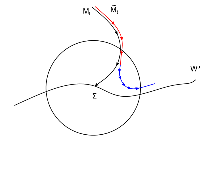
Figure 1. This figure explains the behaviour of the perturbed RMCF $\widetilde{M}_{t}$. In the figure, $M_{t}$ is a RMCF converging to the shrinker $\Sigma$. The circle is the $C^{2,\alpha}$ $\delta$-neighbourhood of $\Sigma$ where the hypersurfaces are graphical on large region of $\Sigma$. The red part of the orbit shows that $\widetilde{M}_{t}$ starts to move to the unstable manifold direction; the blue part of the orbit shows that $\widetilde{M}_{t}$ will move further to the unstable manifold direction, using the invariant cone argument discussed in Section 3.

1.3. Global generic dynamics

To extend the genericity to global dynamics, we need further delicate analysis on the RMCF and the local dynamics.

The dynamical approach of Colding-Minicozzi views the RMCF as the negative gradient flow of the $F$-functional and a shrinker as the fixed point of the RMCF as well as the critical point of $F$. It is natural to linearize the RMCF in a neighborhood of each shrinker and the linearized equation has the form $\partial_{t}u=L_{\Sigma}u$, where

$$L_{\Sigma}=\Delta_{\Sigma}-\frac{1}{2}\langle x,\nabla_{\Sigma}\ \cdot\rangle+(|A|^{2}+1/2)$$

is self-adjoint with respect to the $L^{2}$-inner product $\langle u,v\rangle=\int_{\Sigma}u(x)v(x)e^{-\frac{|x|^{2}}{4}}d\mu.$ The $L_{\Sigma}$-operator also appears naturally as the quadratic form when calculating the second variation of $F$ around a shrinker. An eigenfunction $\phi$ with eigenvalue $\mu$ is a function satisfying the equation $L\phi=\mu\phi$. The eigenfunctions with positive eigenvalues are unstable directions of $F$-functional, and the eigenfunction with the largest eigenvalue represents the most unstable direction. The infinitesimal translations and dilations of $\Sigma$ are eigenfunctions with positive eigenvalues, but the entropy does not decrease if we perturb $\Sigma$ in these directions. So naturally Colding and Minicozzi introduced the notions of $F$-stability and entropy stability to reflect the variational stability modulo the affine transformations [CM1]. From elliptic theory, the eigenfunction with the largest eigenvalue does not change sign. Therefore when $\Sigma$ is not mean convex, infinitesimal translations and dilations are not eigenfunctions with the largest eigenvalue. Thus there must be a positive eigenfunction with an eigenvalue strictly greater than the eigenvalues of infinitesimal translations and dilations, which decreases the entropy of $\Sigma$. Hence a non-mean convex self-shrinker is not entropy stable.

The linearized equation $\partial_{t}u=L_{\Sigma}u$ can be understood easily. To understand the dynamics of the RMCF in a neighborhood of the shrinker, we have to take into account the nonlinearity. The exponential decay given by the negative eigenvalues and the exponential growth given by the positive eigenvalues in the linearized equation represents the hyperbolicity of the system. The invariant manifold theory in the hyperbolic dynamics, in general, gives that the hyperbolicity persists under small perturbations. The dynamics of the RMCF in a neighborhood of the shrinker in general admits stable (unstable) manifold as perturbations of the negative (positive) eigenspace. The existence of invariant manifolds gives detailed information on the local dynamics. To develop the theory of invariant manifold in our setting, a main difficulty is the dependence on the second order derivative in the nonlinearity, which is overcome by using the theory of maximal regularity.

As we have explained before, the invariant manifold theory is only local, and does not give us the existence of a global stable manifold, so the proof of Theorem 1.2 needs essential new ingredients. Suppose we know that a RMCF $(M_{t})$ converging to a closed shrinker, we have to analyze the dynamics of nearby orbits, which leads naturally to the variational equation along the orbit $(M_{t})$

$$\partial_{t}v=L_{M_{t}}v.$$

This can be considered as the Jacobi field equation for the RMCF, which measures the difference of the RMCFs $(M_{t})$ and $(\widetilde{M}_{t})$ where the latter starts from $\widetilde{M}_{0}$ that is a normal graph of the function $\varepsilon v(0)$ over $M_{0}$. This dynamical interpretation of the heat-type equation is crucial for our proof of Theorem 1.2.

The proof of Theorem 1.2 then consists of the following two main steps. First, we develop a Li-Yau estimate to the variational equation to obtain a Harnack estimate for the positive solutions. When time $t=T$ is so large that $M_{t}$ is very close to $\Sigma$, we can identify the $L^{2}$-spaces on $M_{t}$ and $\Sigma.$ Since the leading eigenfunction $\phi_{1}$ of $L_{\Sigma}$ is strictly positive, this implies that $v(t)$ has a nontrivial projection to the $\phi_{1}$-direction. See the red curve in Figure 1. For not necessarily positive initial data, we show that either itself will drift to the first eigenfunction direction, or it drifts to the first eigenfunction after adding a small positive perturbation. In fact, we prove that drifting to the first eigenfunction direction is related to the growth rate of the function (see Lemma 3.12), and we can always make the solution grows sufficiently fast by adding a small positive perturbation.

In the second step, we show that if the difference $M_{T}$ and $\widetilde{M}_{T}$, when considered as a function on $\Sigma$, has a nontrivial projection to the $\phi_{1}$-direction, then the local dynamics will grow the $\phi_{1}$-component exponentially so that it dominates all the other Fourier modes. See the blue curve in Section 1. Thus we get a perturbation towards the $\phi_{1}$-direction on the limit shrinker by a positive perturbation on the initial condition, and [CM1] has proved that such a perturbation will cause entropy decrease.

1.4. Organization of paper

In Section 2, we set up and study the local dynamics. In Section 3, we prove the global genericity and study the RMCF with perturbations on initial data. In Section 4, we discuss how we can see the ancient solution arising from the perturbations on initial data. We also prove the necessary ingredients of the proof in Appendices.

1.5. Notations and conventions

Throughout this paper, whenever we discuss the RMCF, $u$ will be the graph function of a graphical RMCF over the limit shrinker $\Sigma$; $u^{\star}$ will be a solution to the linearized RMCF equation over $\Sigma$; $v$ will be the graph function of a graphical RMCF over the RMCF $M_{t}$, and $v^{\star}$ will be a solution to the linearized RMCF equation over $M_{t}$.

All the Sobolev spaces are defined with respect to Gaussian area. For example

$$\|u\|_{L^{2}(\Sigma)}:=\left(\int_{\Sigma}|u(x)|^{2}e^{-\frac{|x|^{2}}{4}}d\mu\right)^{1/2}.$$

We use the convention that $\lambda$ is an eigenvalue of the linearized operator $L$ if there exists a function $f$ such that $Lf=\lambda f$. We want to remind the readers that this convention is different from many contexts in MCF, such as [CM1]. We adopt this convention for the convenience of studying dynamics since the eigenvalues can be considered as Lyapunov exponents.

Acknowledgement

We would like to thank Professor Tobias Colding and Professor William Minicozzi for stimulating discussions. The work is deeply influenced by their insights. We would like to thank Professor Chongchun Zeng, from whom we learned the theory of maximal regularity. We want to thank Zhihan Wang for the enlightening discussion leading to Theorem 3.11. J.X. is supported by the grant NSFC (Significant project No.11790273) in China and by Beijing Natural Science Foundation (Z180003).

2. The setup and the invariant manifold theorem

Let $\Sigma\subset\mathbb{R}^{n+1}$ be a closed embedded smooth $n$-dimensional shrinker. Then the linearized operator $L:=\Delta_{\Sigma}-\frac{1}{2}\langle x,\nabla\rangle+\frac{1}{2}+|A|^{2}$ has infinitely many negative eigenvalues, finitely many zero eigenvalues and finitely many positive eigenvalues. We call the number of positive eigenvalues the Morse index, denoted by $I$. For a sphere, $I=n+2$; for a nonspherical shrinker, $I>n+2$.

Let $\mathcal{X}$ be the Banach space of the $C^{2,\alpha}$-closure of $C^{\infty}$ functions on $\Sigma$. More explicitly, $\mathcal{X}$ is the space of $C^{2,\alpha}$ functions satisfying in addition $Lu\in h^{\alpha}$ for all $u\in\mathcal{X}$, where

(1) $$h^{\alpha}:=\{u\in C^{\alpha}\ |\ \lim_{r\to 0_{+}}\sup_{|x-y|\leq r}r^{-\alpha}|u(x)-u(y)|=0\}$$

is called the little Hölder space. Each $u\in\mathcal{X}$ gives rise to a hypersurface $\{x+u(x)\mathbf{n}(x):\ x\in\Sigma\}$. We next introduce a splitting on $\mathcal{X}$. We denote by $\phi_{i}$ the eigenfunction of $L$ corresponding to the eigenvalue $\lambda_{i},\ i=1,2,\ldots$ and denote

$$\mathcal{X}^{c}:=\oplus_{\lambda_{i}=0}\phi_{i}\mathbb{R},\quad\mathcal{X}^{u}:=\oplus_{\lambda_{i}>0}\phi_{i}\mathbb{R}$$

We denote by $\Pi_{*}:\ \mathcal{X}\to\mathcal{X}^{*},\ *=c,u$ the $L^{2}$-projection and by $\Pi_{s}:=I-(\Pi_{c}+\Pi_{u})$. We next introduce $\mathcal{X}^{s}:=\Pi_{s}\mathcal{X}$. Let $v=v_{s}+v_{c}+v_{u}\in\mathcal{X}$ be the decomposition with respecting the splitting, then we introduce the norm on $\mathcal{X}$ as $\|v\|_{\mathcal{X}}:=\|v_{s}\|_{C^{2,\alpha}}+\|v_{c}\|_{C^{2,\alpha}}+\|v_{u}\|_{C^{2,\alpha}}$.

Our goal is to show that there exists a stable manifold $\mathcal{W}^{s}$ in $\mathcal{X}$ which can be written as a graph over $\mathcal{X}^{s}$ near zero consisting of points converging to zero as $t\to\infty$, and similarly there exists an unstable manifold $\mathcal{W}^{u}$ as a graph over $\mathcal{X}^{u}$ consisting of points converging to zero as $t\to-\infty$, a center-unstable manifold $\mathcal{W}^{cu}$ as a graph over $\mathcal{X}^{c}\oplus\mathcal{X}^{u}$ and center manifold $\mathcal{W}^{c}$ as a graph over $\mathcal{X}^{c}$. However, in general, the orbits on $\mathcal{W}^{c}$ may not converge to zero under forward or backward flows. In particular, in both the future direction and the past direction, these orbits may escape the small neighborhood where the linear approximation to the RMCF is valid. In general, the way to solve this problem is to choose a truncation of the flow such that outside a small neighborhood of 0 in $E$ the nonlinearity vanishes and the dynamics on the center manifold are trivial. The resulting center manifold of the modified system thus depends on the choice of the truncation which is quite flexible. Meanwhile, in a sufficiently small neighborhood of $0$, the stable and unstable manifolds, as well as those orbits on the center manifold converging to $0$ in the future or the past, do not depend on the truncation.

We choose a truncation as follows. We first pick a $C^{\infty}$ function $\chi:\ \mathbb{R}\to[0,1]$ such that $\chi(x)=1$ for $|x|\in[0,1]$ and $\chi(x)=0$ for $|x|\geq 2$ and $\chi$ is nonincreasing. We pick a small number $\delta>0$ whose value will be fixed below. Denoting the original rescaled mean curvature flow as $\dot{u}=Lu+\mathcal{Q}(u)$, where $\mathcal{Q}$ is given in Section 4 of [CM3]. In the following we work with the following truncated rescaled mean curvature flow ($\mathrm{TRMCF}$)

(2) $$\dot{u}=Lu+\chi(u/{\delta})\mathcal{Q}(u):=Lu+f(u).$$

We denote by $\Phi^{t}$ the flow generated by this equation.

The main theorem that we prove in this section is as follows.

Theorem 2.1.

Let $\Sigma^{n}$ be a smooth closed embedded shrinker in $\mathbb{R}^{n+1}$. Then there exists a sufficiently small $\delta$ such that in the $\delta$-ball $B_{\delta}(0)$ of $\mathcal{X}$, the following hold:

1. There is a Lipschitz manifold $\mathcal{W}^{s}$ that is the graph of a function $w^{s}:\ \mathcal{X}^{s}\cap B_{\delta}(0)\to\mathcal{X}^{c}\oplus\mathcal{X}^{u}$, with $w^{s}(0)=0$, $T_{0}\mathcal{W}^{s}=\mathcal{X}^{s}$, and every point on $\mathcal{W}^{s}$ has its forward orbit under the RMCF converges to $0$ exponentially.

2. There is a Lipschitz manifold $\mathcal{W}^{u}$ of dimension $I$, that is the graph of a function $w^{u}:\ \mathcal{X}^{u}\cap B_{\delta}(0)\to\mathcal{X}^{s}\oplus\mathcal{X}^{c}$, with $w^{u}(0)=0$, $T_{0}\mathcal{W}^{u}=\mathcal{X}^{u}$, and every point on $\mathcal{W}^{u}$ has its backward orbit under the RMCF converges to $0$ exponentially.

3. There is a Lipschitz manifold $\mathcal{W}^{cu}$ of finite dimension that is the graph of a function $w^{cu}:\ \mathcal{X}^{c}\oplus\mathcal{X}^{u}\cap B_{\delta}(0)\to\mathcal{X}^{s}$, with $w^{cu}(0)=0$, $T_{0}\mathcal{W}^{cu}=\mathcal{X}^{c}\oplus\mathcal{X}^{u}$. Moreover, there exist constants $C>0,\eta>0,$ such that for each orbit $u(t)$ of the TRMCF within $B_{\delta}$ we have the estimate

   $$\|\Pi_{s}u(t)-w^{cu}(\Pi_{cu}u(t))\|_{C^{2,\alpha}}\leq Ce^{-\eta t}\|\Pi_{s}u(0)-w^{cu}(\Pi_{cu}u(0))\|_{C^{2,\alpha}}.$$

4. There is a Lipschitz manifold $\mathcal{W}^{c}$ that is invariant under the TRMCF, and is the graph of a function $w^{c}:\ \mathcal{X}^{c}\cap B_{\delta}(0)\to\mathcal{X}^{s}\oplus\mathcal{X}^{u}$, with $w^{c}(0)=0$, $T_{0}\mathcal{W}^{c}=\mathcal{X}^{c}$.

Remark 2.1.

We have the following remarks.

1. This result generalizes the result of [EW] from rescaled curve shortening flow to MCF.

2. In Proposition 2.3 of [CM3], Colding-Minicozzi constructed a stable object $W$ whose manifold structure is unknown. The paper [CM3] has an important feather that is to modulo the Euclidean affine transformation group, which can also be incorporated into our local analysis here. We refer readers to [CM3] for more details.

3. In [ChM], Choi-Mantoulidis proved that for compact self-shrinkers the existence of ancient solutions that forms an $I$-parameter family where $I$ is the dimension of positive eigenvalues counting multiplicity. Our theorem recovers their result and proves, in addition, the manifold structure of these ancient solutions in the function space $C^{2,\alpha}$.

We next work on the proof of this theorem. As we have remarked in the introduction, the presence of the $\nabla^{2}u$ term in the nonlinearity makes the DuHamel principle not give a smooth solution to the RMCF equation. We invoke the theory of maximal regularity to remedy this situation by introducing certain interpolation spaces. The proof is adapted from [DL].

Definition 2.2.

Let $X$ be a Banach space and $D\subset X$ be a continuous embedding. An operator $L:\ D\to X$ is said to be sectorial if there exist constants $\omega\in\mathbb{R},\ \theta\in(\frac{\pi}{2},\pi),\ M>0$ such that the following hold:

1. the resolvent set of $L$ contains the sector $S:=\{\lambda\in\mathbb{C}\ |\ \lambda\neq\lambda_{0},\ |\mathrm{arg}(\lambda-\lambda_{0})|<\theta\}$;

2. $\|R(\lambda,L)\|_{L(X)}\leq\frac{M}{|\lambda-\lambda_{0}|},$ for all $\lambda\in S$, where $R(\lambda,L)=(\lambda-L)^{-1}$ is the resolvent.

Let $\bar{\lambda}=\sup\{\mathrm{Re}\lambda\ |\ \lambda\in\sigma(L)\}$ and $\omega$ be a number greater than $\bar{\lambda}$, and $L(X)$ be the space of linear operators densely defined on $X$ equipped with operator norm.

Lemma 2.3.

Let $L:\ D\to X$ be a sectorial operator. Then it generates an analytic semigroup $e^{tL}$ and there exist constants $C_{0},C_{1}$ such that for all $t>0$

$$\|e^{tL}\|_{L(X)}\leq C_{0}e^{\omega t},\quad\|Le^{tL}\|_{L(X)}\leq\frac{C_{1}}{t}e^{\omega t},$$

The proof of this lemma can be found in Proposition 2.1.1 of [Lu2].

In the following, we shall choose the operator $L$ to be $L:=L_{\Sigma}$ and three different choices of the pair $(D,X)$: $(C^{2}(\Sigma),C^{0}(\Sigma))$, $(C^{2,\alpha}(\Sigma),C^{\alpha}(\Sigma))$ and $(h^{2,\alpha}(\Sigma),h^{\alpha}(\Sigma))$, where $h^{\alpha}$ is the little Hölder space defined in (1) and $h^{2,\alpha}=\mathcal{X}$ is the space of functions such that $Lu\in h^{\alpha}$ for $u\in h^{2,\alpha}$. We shall choose $0<\alpha<1/2$ in the sequel. The sectorality of the operator $L$ on these three pair of spaces is proved in [Lu2] Theorem 3.1.14 and Corollary 3.1.32.

The following result gives an important characterization of the Hölder and little Hölder spaces in terms of the semigroup $e^{tL}$.

Proposition 2.4.

1. The $C^{\alpha}(\Sigma)$ space is norm equivalent to the space

   $$\mathcal{E}_{\alpha/2}:=\{u\in C^{0}(\Sigma)\ |\ \|u\|_{\alpha/2}<\infty\}$$

   where the norm $\|\cdot\|_{\alpha/2}$ is defined to be $\|u\|_{\alpha/2}:=\sup_{\xi>0}\xi^{1-\alpha/2}\|Le^{\xi L}u\|_{C^{0}}$ when $\omega<0$. In case of $\omega>0$, we replace $L$ by $L-2\omega$.

2. The $C^{2,\alpha}(\Sigma)$ space is norm equivalent to the space

   $$\mathcal{E}_{1+\alpha/2}:=\{u\in C^{2}(\Sigma)\ |\ \|Lu\|_{\alpha/2}<\infty\}$$

   and the norm $\|\cdot\|_{1+\alpha/2}=\|\cdot\|_{\alpha/2}+\|L\cdot\|_{\alpha/2}$.

3. The $h^{\alpha}(\Sigma)$ space is norm equivalent to the closure of $C^{2}(\Sigma)$ in the $\|\cdot\|_{\alpha/2}$ norm and the $h^{2,\alpha}(\Sigma)$ space is norm equivalent to the space of $C^{2}$ functions with $Lu\in h^{\alpha}$, $u\in C^{2}$.

The proof of these results can be found in Theorem 2.10 of [Lu1] and Chapter 3 (Theorem 3.1.12, 3.1.29, 3.1.30) of [Lu2].

We next study the RMCF equation using the theory of maximal regularity. We first formally write down the solution to the RMCF equation

(3) $$u(t)=e^{Lt}u_{0}+\int_{0}^{t}e^{L(t-s)}f(u(s))\,ds:=e^{Lt}u_{0}+V(t,u).$$

We have the following crucial proposition, which consists of Proposition 1.1 and 1.2 of [DL]). We include a proof since it is illuminating.

Proposition 2.5.

1. Let $f\in C([0,T),h^{\alpha})$, $T\in(0,\infty]$ be such that $\sup_{t\in[0,T)}\|e^{\eta t}f(t)\|_{C^{\alpha}}<\infty$. Let $\eta$ be such that $\eta+\omega<0$. Then we have

   $$\sup_{t\in[0,T)}\|e^{\eta t}\partial_{t}u(t)\|_{C^{\alpha}}+\sup_{t\in[0,T)}\|e^{\eta t}V(t,u)\|_{C^{2,\alpha}}\leq C\sup_{t\in[0,T)}\|e^{\eta t}f(t)\|_{C^{\alpha}}.$$

2. Suppose $f\in C((-\infty,0],h^{\alpha})$ with $\sup_{t}e^{\eta t}\|f(t)\|_{C^{\alpha}}<\infty$, where $\eta$ satisfies $\eta+\omega<0$. Denote $V_{-\infty}(t,u)=\int_{-\infty}^{t}e^{L(t-s)}f(u(s))\,ds$. Then we have

   $$\sup_{t\in\mathbb{R}_{\leq 0}}\|e^{\eta t}V_{-\infty}(t,u)\|_{C^{2,\alpha}}\leq C\sup_{t\in\mathbb{R}_{\leq 0}}\|e^{\eta t}f(t)\|_{C^{\alpha}}.$$

Proof.

We only give the proof of item (1), and that of item (2) is completely similar. We consider first the case of $\eta=0$. Using Proposition 2.4, we have

$$\|V(t,u)\|_{C^{2,\alpha}} \leq C\|V(t,u)\|_{1+\alpha/2}=C\|LV(t,u)\|_{\alpha/2}$$

$$=C\sup_{\xi}\left\|\xi^{1-\alpha/2}\int_{0}^{t}L^{2}e^{(\xi+t-s)L}f(u(s))\,ds\right\|_{\alpha/2}$$

$$=C\sup_{\xi}\xi^{1-\alpha/2}\int_{0}^{t}\left\|Le^{\frac{(\xi+t-s)}{2}L}Le^{\frac{(\xi+t-s)}{2}L}f(u(s))\right\|_{C^{0}}\,ds$$

$$\leq C\sup_{\xi}\xi^{1-\alpha/2}\int_{0}^{t}(\frac{\xi+t-s}{2})^{-1}\|Le^{\frac{(\xi+t-s)}{2}L}f(u(s))\|_{C^{0}}\,ds$$

$$\leq C\sup_{t}\|f(t)\|_{\alpha/2}\cdot\sup_{\xi}\int_{0}^{t}\xi^{1-\alpha/2}(\frac{\xi+t-s}{2})^{-2+\alpha/2}\,ds$$

$$\leq C\sup_{t}\|f(t)\|_{C^{\alpha}},$$

where in the second $\leq$, we use Lemma 2.3 and the fact $\omega<0$, and in the third $\leq$, we use the definition of the $\|\cdot\|_{\alpha/2}$ norm.

We next consider the case of general $\omega$ and $\eta$. We shall substitute $f_{\eta}(t)=e^{\eta t}$ and $L_{\eta}=L+\eta$. Then we reduce the general case to the above case. ∎

We next verify the regularity of the nonlinear term in (2).

Lemma 2.6.

The function $f:\ h^{2,\alpha}\to h^{\alpha}$ defined by $f(u):=F(x,u,\nabla u,\nabla^{2}u)=\chi(u/\delta)\mathcal{Q}(u)$ is uniformly Lipschitz: $\frac{\|f(u)-f(v)\|_{C^{\alpha}}}{\|u-v\|_{C^{2,\alpha}}}\leq C$. Moreover, the Lipschitz constant approaches zero as $\delta\to 0$.

Proof.

The explicit expression of $F$ is provided in [CM3] as well as [CCMS1]. Indeed, by fundamental theorem of calculus, we have

$$f(u)-f(v)= \left(\int_{0}^{1}\partial_{2}F(x,t\mathbf{u}+(1-t)\mathbf{v})dt\right)(u-v)+\left(\int_{0}^{1}\partial_{3}F(x,t\mathbf{u}+(1-t)\mathbf{v})dt\right)(\nabla u-\nabla v)$$

$$+\left(\int_{0}^{1}\partial_{4}F(x,t\mathbf{u}+(1-t)\mathbf{v})dt\right)(\nabla^{2}u-\nabla^{2}v)$$

where $\partial_{i}$ means the partial derivative with respect to the $i$-th variable of $F$, $i=2,3,4$ and $\mathbf{u}=(u,\nabla u,\nabla^{2}u),\ \mathbf{v}=(v,\nabla v,\nabla^{2}v)$. The statement of the lemma follows from the fact that $\partial_{i}F:h^{2,\alpha}\to h^{\alpha}$ is smooth. ∎

We are now ready to give the proof of Theorem 2.1.

Proof of Theorem 2.1 .

(1) We first show how to construct the stable manifold $\mathcal{W}^{s}$. Let $\mathcal{X}$ with the splitting $\mathcal{X}=\mathcal{X}^{s}\oplus\mathcal{X}^{c}\oplus\mathcal{X}^{u}$ be as in the statement. Let us further denote by $X_{1}=\mathcal{X}^{s}$ and $X_{2}=\mathcal{X}^{c}\oplus\mathcal{X}^{u}$, and denote by $\Pi_{i}$ the $L^{2}$ projection $\mathcal{X}$ to $X_{i}$, $i=1,2$. Instead of considering the operator $L$, we perturb it to $L+\varepsilon$ for some small $\varepsilon>0$. The perturbation is to make sure that $L+\varepsilon|_{X_{2}}$ has positive spectrum and $L+\varepsilon|_{X_{1}}$ has negative spectrum, which gives certain expansion on $X_{2}$ and contraction on $X_{1}$ for the semigroups. We will fix $\varepsilon$ in the following. We next denote by $L_{i}$ the restriction of $L+\varepsilon$ to $X_{i}$ when $i=1,2$. So the eigenvalues of $L_{1}$ are all negative and that of $L_{2}$ are all positive. We introduce $\omega_{1}<0$ and $\omega_{2}>0$ such that $\omega_{1}>\sup\{\sigma(L_{1})\}$ and $\omega_{2}>\sup\{\sigma(L_{2})\}$.

Note that $X_{2}$ is a finite dimensional space and $L_{2}$ is a finite dimensional linear operator, so we have for $u\in X_{2}$

(4) $$\|e^{L_{2}t}u\|_{1+\alpha/2} =\|Le^{L_{2}t}u\|_{\alpha/2}=\|L_{2}e^{L_{2}t}u\|_{\alpha/2}=\sup_{\xi}\xi^{1-\alpha}\|L_{2}^{2}e^{\xi L_{2}}e^{tL_{2}}u\|_{C^{0}}$$

$$\leq Ce^{\omega_{2}t}\sup_{\xi}\xi^{1-\alpha}\|L_{2}e^{\xi L_{2}}u\|_{C^{0}}=Ce^{\omega_{2}t}\|u\|_{\alpha/2}.$$

Let $u_{1}(0)\in X_{1}$ with $\|u_{1}(0)\|_{1+\alpha/2}<d$ for some sufficiently small $d$ to be determined later. We next introduce the operator

$$\Lambda u =e^{L_{1}t}u_{1}(0)+\int_{0}^{t}e^{(t-s)L_{1}}\Pi_{1}(e^{\varepsilon s}f(e^{-\varepsilon s}u(s)))\,ds$$

$$-\int_{t}^{\infty}e^{(t-s)L_{2}}\Pi_{2}(e^{\varepsilon s}f(e^{-\varepsilon s}u(s)))\,ds.$$

We next show that for small $a>0,$ the operator $\Lambda:\ \ Y_{a}\to Y_{a}$ is a contraction hence has a fixed point, where $Y_{a}$ is defined as the set

$$Y_{a}=\{z\in C(\mathbb{R}_{\geq 0},h^{2,\alpha})\ |\ \sup_{t\geq 0}e^{\eta t}\|z(t)\|_{1+\alpha/2}<a\},$$

where $\eta$ is a small positive number such that $\omega_{1}+\eta<0$. It is straightforward to check that a fixed point of $\Pi$ is a solution to the differential equation $\partial_{t}u=(L+\varepsilon)u+e^{\varepsilon t}f(e^{-\varepsilon t}u)$, hence $v=e^{-\varepsilon t}u$ is a solution of the equation $\partial_{t}v=Lv+f(v)$ with the same initial condition $u(0)=v(0)$.

We first show that $\Lambda$ is a map from $Y_{a}$ to $Y_{a}$ if we choose $d$ and $a$ sufficiently small. By Lemma 2.6 and by choosing $d$ small, we suppose $f:\ h^{2,\alpha}\cap B_{d}\to h^{\alpha}$ is $\delta$-Lipschitz where $B_{d}$ is the $d$-ball in $h^{2,\alpha}$.

Take $u\in Y_{a}$, then it is clear that $e^{-\varepsilon t}u(t)\in h^{2,\alpha}$ for all $t\geq 0$ by the definition of $Y_{a}$. We have

$$\|e^{\eta t}\Lambda u(t)\|_{1+\alpha}\leq C_{0}\|u_{1}(0)\|_{1+\alpha/2}+\sup_{t}\|e^{\eta t}\Pi_{1}e^{\varepsilon t}f(e^{-\varepsilon t}u(t))\|_{\alpha/2}$$

$$+\int_{t}^{\infty}Ce^{-\varepsilon(t-s)}e^{\eta s}\|\Pi_{2}e^{\varepsilon s}f(e^{-\varepsilon s}u(s))\|_{\alpha/2}\,ds$$

$$\leq C_{0}\|u_{1}(0)\|_{1+\alpha/2}+\delta\sup_{t}\|e^{\eta t}u(t)\|_{1+\alpha/2}+\frac{C\delta}{\varepsilon}\sup_{t}\|e^{\eta t}u(t)\|_{1+\alpha/2}$$

$$\leq C_{0}d+\frac{C\delta}{\varepsilon}a.$$

where in the first $\leq$ we use Lemma 2.3, Proposition 2.5 and (4), and in the second $\leq$, we use Lemma 2.6. For given $\varepsilon$, we choose $\delta$ and $d$ sufficiently small to get that $\Lambda u(t)\in Y_{a}$.

We next prove the contraction. Taking $u,v\in Y_{a}$ with the same initial condition $u_{1}(0)$ gives that

(5) $$\|e^{\eta t}\Lambda u(t)-e^{\eta t}\Lambda v(t)\|_{1+\alpha/2}$$

$$\leq\|e^{\eta t}\int_{0}^{t}e^{(t-s)L_{1}}\Pi_{1}(e^{\varepsilon s}f(e^{-\varepsilon s}u(s))-e^{\varepsilon s}f(e^{-\varepsilon s}v(s)))\,ds\|_{1+\alpha/2}$$

$$+e^{\eta t}\|\int_{t}^{\infty}e^{(t-s)L_{2}}\Pi_{2}(e^{\varepsilon s}f(e^{-\varepsilon s}u(s))-e^{\varepsilon s}f(e^{-\varepsilon s}v(s)))\,ds\|_{1+\alpha/2}$$

$$\leq C\sup_{t}\|e^{\eta t}\Pi_{1}e^{\varepsilon s}f(e^{-\varepsilon s}u(t))-\Pi_{1}e^{\varepsilon s}f(e^{-\varepsilon s}v(t))\|_{\alpha/2}$$

$$+C\int_{t}^{\infty}e^{\eta s}e^{(t-s)\varepsilon}\|\Pi_{2}(e^{\varepsilon s}f(e^{-\varepsilon s}u(s))-e^{\varepsilon s}f(e^{-\varepsilon s}v(s)))\|_{\alpha/2}\,ds$$

$$\leq C_{\varepsilon}\sup_{t}\|e^{\eta t}e^{\varepsilon s}f(e^{-\varepsilon s}u(t))-e^{\varepsilon s}f(e^{-\varepsilon s}v(t))\|_{\alpha/2}$$

$$\leq C_{\varepsilon}\delta\sup_{t}\|e^{\eta t}(u(t)-v(t))\|_{1+\alpha/2}$$

where in the second $\leq$, we use Proposition 2.5 and (4), and in the fourth $\leq$, we use Lemma 2.6.

The contraction implies that there exists a fixed point $u=\Lambda u$ with initial condition $u(0)=u_{1}(0)+\int_{0}^{\infty}e^{-sL_{2}}\Pi_{2}(e^{\varepsilon s}f(e^{-\varepsilon s}u(s)))ds$. We define the map

$$w^{s}:u_{1}(0)\mapsto\int_{0}^{\infty}e^{-sL_{2}}\Pi_{2}(e^{\varepsilon s}f(e^{-\varepsilon s}u(s))).$$

Repeating the calculation in (5), we see that the map $u_{1}(0)\mapsto u(t)$ going from $X_{1}\cap B_{d}$ to $Y_{a}$ is Lipschitz, i.e. we have

$$(1-C\delta)\sup_{t}\|e^{\eta t}(u(t)-v(t))\|_{1+\alpha/2}\leq C\|u_{1}(0)-v_{1}(0)\|_{1+\alpha/2}.$$

Then using the expression of $w^{s}$, we get

$$\|w^{s}(u_{1}(0))-w^{s}(v_{1}(0))\|_{1+\alpha/2}\leq C_{\varepsilon}\delta\sup_{t}\|e^{\eta t}(u(t)-v(t))\|_{1+\alpha/2}\leq C_{\varepsilon}\delta\|u_{1}(0)-v_{1}(0)\|_{1+\alpha/2}.$$

This means that $w^{s}$ is a $C\delta$-Lipschitz function and in particular is differentiable at zero. Then we realize the stable manifold $\mathcal{W}^{s}$ as the graph of $w^{s}$ over $X_{1}\cap B_{d}$. This proves part (1) of the theorem.

(2) To construction the unstable manifold, we consider instead the operator $L-2\varepsilon$ and introduce the spaces $X_{i}$ and $L_{i}$ according to the signs of the spectrum of $L-2\varepsilon$ similar as above. Taking $u_{2}(0)\in X_{2}$ with norm less than $d$, we introduce the following operator

$$\Lambda u =e^{L_{2}t}u_{2}(0)+\int_{0}^{t}e^{(t-s)L_{2}}\Pi_{2}(e^{-\varepsilon s}f(e^{\varepsilon s}u(s)))\,ds$$

$$+\int^{t}_{-\infty}e^{(t-s)L_{1}}\Pi_{1}(e^{-\varepsilon s}f(e^{\varepsilon s}u(s)))\,ds$$

and the space

$$Y_{a}=\{z\in C(\mathbb{R}_{\leq 0},h^{2,\alpha})\ |\ \sup_{t\leq 0}e^{-\eta t}\|z(t)\|_{1+\alpha/2}<a\}$$

where $\eta>0$ is such that $\eta-\bar{\omega}_{2}<0,\ \bar{\omega}_{2}=\sup\{\sigma(-L_{2})\}.$ We can then repeat the above argument to show that $\Lambda$ has a fixed point in $Y_{a}$. Hence the unstable manifold is constructed similarly. This proves part (2).

(3) The existence of a center-unstable manifold needs a slight variant of the above argument. We refer readers to Theorem 3.1 and 3.3 of [DL]. This gives part (3).

(4) We next work on the center manifold. We use the splitting $\mathcal{X}=\mathcal{X}^{s}\oplus\mathcal{X}^{c}\oplus\mathcal{X}^{u}$ and introduce the projections $\Pi_{*}:\ \mathcal{X}\to\mathcal{X}^{*}$ and the operators $L_{*}=L|_{\mathcal{X}^{*}},\ *=s,c,u.$ Let $u_{c}(0)\in\mathcal{X}^{c}$ with norm $\|u_{c}(0)\|_{1+\alpha/2}<d$ for some small $d$ to be determined later. We introduce the operator:

$$\Lambda_{c}u =u_{c}(0)+\int_{-\infty}^{t}e^{(t-s)L_{s}}\Pi_{s}(f(u(s)))\,ds+\int_{0}^{t}\Pi_{c}(f(u(s)))\,ds$$

$$-\int_{t}^{\infty}e^{(t-s)L_{u}}\Pi_{u}(f(u(s)))\,ds$$

defined on the space of slowing growing functions in both the future and the past

$$Y_{a}=\{z\in C(\mathbb{R},h^{2,\alpha})\ |\ \sup_{t\in\mathbb{R}}e^{-\eta|t|}\|z(t)\|_{1+\alpha/2}<a\}$$

where $\eta>0$ is a small number. We first show that $\Lambda_{c}$ maps $Y_{a}$ to $Y_{a}$. For simplicity, we do the estimate for $t\geq 0$. To do the similar argument for $t\leq 0$, it is enough to change $\eta$ to $-\eta$

$$\|e^{-\eta t}\Lambda_{c}u\|_{1+\alpha/2}$$

$$\leq\|e^{-\eta t}u_{c}(0)\|_{1+\alpha/2}+\left\|e^{-\eta t}\int_{-\infty}^{t}e^{(t-s)L_{s}}\Pi_{s}(f(u(s)))\,ds\right\|_{1+\alpha/2}$$

$$+\left\|e^{-\eta t}\int_{0}^{t}\Pi_{c}(f(u(s)))\,ds\right\|_{1+\alpha/2}+\left\|e^{-\eta t}\int_{t}^{\infty}e^{(t-s)L_{u}}\Pi_{u}(f(u(s)))\,ds\right\|_{1+\alpha/2}$$

$$\leq C\|u_{c}(0)\|_{1+\alpha}+\left\|e^{-\eta t}\Pi_{s}(f(u(t)))\right\|_{\alpha/2}+\left\|e^{-\eta t}\int_{0}^{t}\Pi_{c}(f(u(s)))\,ds\right\|_{\alpha/2}$$

$$+e^{-\eta t}\int_{t}^{\infty}e^{(t-s)\omega_{2}}\|\Pi_{u}(f(u(s)))\|_{\alpha/2}\,ds$$

$$\leq C\|u_{c}(0)\|_{1+\alpha}+\delta\left\|e^{-\eta t}u(t)\right\|_{1+\alpha/2}+e^{-\eta t}\int_{0}^{t}\delta e^{\eta s}\sup_{s}(e^{-\eta s}\left\|u(s)\right\|_{1+\alpha/2})\,ds$$

$$+e^{-\eta t}\int_{t}^{\infty}e^{(t-s)\omega_{2}}e^{\eta s}\delta\sup_{s}(e^{-\eta s}\|u(s)\|_{1+\alpha/2})\,ds$$

$$\leq C\|u_{0}(0)\|_{1+\alpha/2}+C\delta\sup_{s}(e^{-\eta s}\|u(s)\|_{1+\alpha/2}).$$

By choosing $a$ and $\|u_{0}(0)\|_{1+\alpha/2}$ small, we prove that $\Lambda_{c}$ maps $Y_{a}$ to $Y_{a}$. Similarly, we show that $\Lambda_{c}:\ Y_{a}\to Y_{a}$ is a contraction. The contraction yields a fixed point. The center manifold can be constructed similar to the stable manifold. This gives part (4). ∎

3. The global genericity theorem

In this section, we prove Theorem 1.2.

3.1. The variational equation and its main properties

Let $(M_{t})_{t\in[0,T]}$ be a smooth solution to the RMCF $x_{t}=-(H-\frac{\langle x,\mathbf{n}\rangle}{2})\mathbf{n}$ on the time interval $[0,T]$. Let $E(t)$ be the  Banach space of $C^{2,\alpha}$ functions on $M_{t},\ t\in[0,T]$. Thus each sufficiently small $v(t)\in E(t)$ gives rise to a hypersurface $N^{v(t)}:=\{x+v(t)\mathbf{n}_{t}(x)\ |\ x\in M_{t}\}$ where $\mathbf{n}_{t}$ is the outer normal vector field on $M_{t}$.

Let $\varepsilon v(0)\in E(0)$, which gives rise to a hypersurface $N^{\varepsilon v(0)}$ that is a graph over $M_{0}$. Flow $N^{\varepsilon v(0)}$ by the RMCF over time $[0,T]$ and denote by $(N_{\varepsilon,t})_{t\in[0,T]}$ this RMCF. Since there is no singularity of $(M_{t})$ on the time interval $[0,T]$, so is the flow $N_{\varepsilon,t}$ if $\varepsilon$ is sufficiently small, by the local well-posedness of the RMCF (c.f. Proposition 3.1). Denoting

$$N_{\varepsilon,t}=M_{t}+v_{\varepsilon}(t)\mathbf{n}_{t},\quad v_{\varepsilon}(t)\in E(t),$$

where the difference is taken along the outer normal $\mathbf{n}_{t}$ of $M_{t}$.

We let $\varepsilon\to 0$ and denote $\lim_{\varepsilon\to 0}\frac{v_{\varepsilon}(t)}{\varepsilon}=v^{\star}(t)$. Then to the leading order we obtain formally a linear equation called variational equation governing the evolution of $v^{\star}$. Explicitly, the variational equation reads (See Appendix A for the derivation. Also c.f. [CM3], Theorem 4.1, equation (4.7), (4.8))

$$\partial_{t}v^{\star}(t)=L_{M_{t}}v^{\star}(t),$$

where $L_{M_{t}}:=\Delta_{M_{t}}-\frac{1}{2}\langle x,\nabla_{M_{t}}\rangle+(|A|^{2}+\frac{1}{2})$ is the linearized operator associated to the hypersurface $M_{t}$. This equation is also called linearized RMCF equation or simply linearized equation.

We next study some basic properties of the variational equation.

Proposition 3.1.

Given a RMCF $M_{t}$ converging to a closed self-shrinker $\Sigma$, there exists $\delta_{0}>0$, $\alpha^{\prime}>0,\varepsilon_{0}>0$ and $C$ so that if $v_{0}:M_{T}\to\mathbb{R}$, for all $T\geq 0,$ satisfies

$$|v_{0}|+|\nabla v_{0}|\leq\delta\leq\delta_{0},\quad|\mathrm{Hess}_{v_{0}}|\leq 1,$$

then there exists a solution to the RMCF equation $v:\ \cup_{t\in[T,T+\varepsilon_{0}]}M_{t}\times\{t\}\to\mathbb{R}$ with $v(\cdot,T)=v_{0}$ and

• $|v|\leq C\delta$, $|\mathrm{Hess}_{v}|\leq C$, and $|\nabla v|^{2}\leq C\delta$ on $\cup_{t\in[T,T+\varepsilon_{0}]}M_{t}\times\{t\}$.

• $\|v(\cdot,T+\varepsilon_{0})\|_{C^{2,\alpha^{\prime}}}\leq C$.

• Given $\alpha\in[0,\alpha^{\prime})$, we have $\|v(\cdot,T+\varepsilon_{0})\|_{C^{2,\alpha}}\leq C\delta^{\frac{\alpha^{\prime}-\alpha}{2+\alpha^{\prime}}}.$

This proposition is an analogue of Proposition 3.28 of [CM3]. In Appendix A.1, we will work out the equations of motion for $N_{t}$ written as a graph of $v$ over a given RMCF $M_{t}$. After that, the proposition is proved by repeating the argument in Section 3 of [CM3]. We refer readers to Appendix A.1 and [CM3] for more details.

Suppose $v:\ M_{t}\to\mathbb{R}$ is such that $N^{v(t)}$ is a RMCF close to $M_{t}$ for some short time, and $v^{\star}$ satisfies the linearized equation on $M_{t}$. Define $w=v-v^{\star}$. Then $w$ satisfies the equation

$$\partial_{t}w=L_{M_{t}}w+\mathcal{Q}(v).$$

Notice that $\mathcal{Q}$ is of quadratic from the above proposition and the estimate in [CM3] (Lemma 3.5), see also Appendix A.1. Then from the parabolic Schauder theorem and previous analysis of the RMCF equation, we get the following proposition characterizing the difference between the RMCF and linearized equation in Hölder norm.

Proposition 3.2.

Given a RMCF $\{M_{t}\}_{t\in[0,\infty)}$ converging to a closed self-shrinker $\Sigma$ and $T>0$, there exists $\delta_{0}>0$, $\epsilon_{0}>0$ and $C$ so that, if $v(0):M_{0}\to\mathbb{R}$ satisfies

$$|v(0)|+|\nabla v(0)|\leq\delta\leq\delta_{0},\quad|\mathrm{Hess}_{v(0)}|\leq 1,$$

Then we have for $t\in[1,T]$

$$\|(v-v^{\star})(\cdot,t)\|_{C^{2,\alpha}}\leq C\delta^{1+\epsilon_{0}}.$$

The variational equation is a time-dependent linear parabolic equation. We are interested in its solutions with positive initial conditions. By the maximum principle, the solution remains positive for all time. Finer information about positive solutions is given by the following Li-Yau estimate and Harnack inequality. Since they are of independent interest, we study them systematically in Appendix B. The following is the analogous theorem in our setting.

Theorem 3.3.

Let $\{M_{t}\}_{t\in[0,1]}$ be a RMCF and $v^{\star}$ be a positive solution to the variational equation $\partial_{t}v^{\star}=L_{M_{t}}v^{\star}$. Then there exists $\delta>0$ and $C>0$ depending on $(M_{t})_{t\in[0,1]}$, such that

$$\partial_{t}(\log v^{\star})\geq\frac{|\nabla\log v^{\star}|^{2}}{2}-C-\frac{C}{t}\quad\text{on $(0,4\delta)$}.$$

Compared with the standard Li-Yau estimate in [LY], our Li-Yau estimate deals with the Bakry-Emery Laplacian $\Delta_{M_{t}}-\langle x,\nabla\rangle$ with a potential $|A|^{2}+\frac{1}{2}$. Our result differs from existing results (for instance [Lee, Li]) in that our $L_{M_{t}}$ operator is time-dependent.

The next ingredient is the following Harnack inequality. In general, the Harnack inequality derived from the Li-Yau estimate can only compare oscillations of solutions on different time slices, and the estimate blows up on the same time slice. The following Harnack inequality allows us to estimate the oscillation of positive solutions on each time slice.

Theorem 3.4.

Let $\{M_{t}\}_{t\in[0,\infty)}$ be a RMCF converging to a compact shrinker $\Sigma$ smoothly. There exist $\widetilde{t}>0$, $C>0$ such that the following is true: let $v^{\star}$ be a positive solution to the RMCF equation $\partial_{t}v^{\star}=L_{M_{t}}v^{\star}$ on the time interval $[0,\infty)$, then we have

$$\max v^{\star}(\cdot,t)\leq C\min v^{\star}(\cdot,t),\quad\forall\ t\geq\widetilde{t}.$$

We are interested in the case of $M_{t}\to\Sigma$ under the RMCF where $\Sigma$ is a compact shrinker. For $t$ sufficiently large, we assume that $M_{t}$ is sufficiently close to $\Sigma$ in the $C^{k}$ topology for any $k\geq 4$ so we can write $M_{t}$ as a graph over $\Sigma$. In fact, even only a subsequence of $M_{t}$ converge to $\Sigma$ in Lipschitz norm, the uniqueness of tangent flow proved by Schulze in [Sc] shows that $M_{t}$ converges to $\Sigma$ smoothly, independent the choice of subsequence.

Theorem 3.3 and Theorem 3.4 are proved in Appendix B.

At time $t$, a solution to the variational equation, is a function on $M_{t}$. We would like to apply the invariant manifold theory in a small neighborhood of the shrinker. For this purpose, when $t$ sufficiently large, we would like to write the graph of a function $v$ on $M_{t}$ as a graph over $\Sigma$. So we introduce the notion of transplantation.

Definition 3.5 (Transplantation).

Let $\Sigma$ be a closed embedded hypersurface and $\Sigma^{\prime}$ be a graph of function $f$ over $\Sigma$. Given a function $u$ on $\Sigma^{\prime}$, we say that $\bar{u}:\ \Sigma\to\mathbb{R}$ is a transplantation of $u$, if $\bar{u}(x)=u(x+f(x)\mathbf{n}(x))$.

We have the following theorem relating graphs on $M_{t}$ and graphs on the shrinker $\Sigma$.

Theorem 3.6.

Let $\Sigma$ be a fixed embedded closed hypersurface. Then given $\varepsilon>0$, there exists a constant $\mu(\varepsilon)>0$ with $\mu(\varepsilon)\to 0$ as $\varepsilon\to 0$, such that the following is true: Suppose

1. $\Sigma_{1}$ is the graph $\{x+f(x)\mathbf{n}(x):x\in\Sigma\}$ over $\Sigma$,

2. and $\Sigma_{2}$ is the graph $\{y+g(y)\mathbf{n}(y):y\in\Sigma_{1}\}$ over $\Sigma_{1}$,

3. and $\|f\|_{C^{4}(\Sigma)}\leq\mu$, $\|g\|_{C^{2,\alpha}(\Sigma_{1})}\leq\mu$,

then $\Sigma_{2}$ is a graph of a function $v$ on $\Sigma$, and

$$\|v-(f+\bar{g})\|_{C^{2,\alpha}(\Sigma)}\leq\varepsilon\|\bar{g}\|_{C^{2,\alpha}(\Sigma)}$$

where $\bar{g}(x)=g(x+f(x)\mathbf{n}(x))$ is the transplantation of $g$ to $\Sigma$.

This theorem will be proved in Appendix C.

Combining all the ingredients above we can prove that, after a sufficiently long time, the positive solution (after transplantation) to the linearized equation on $M_{t}$ will be close to the first eigenfunction direction on the limit shrinker. Let $\phi_{1}$ be the eigenfunction associated to the leading eigenvalue of the operator $L_{\Sigma}$, and we define $\Pi_{\phi_{1}}$ to be the $L^{2}$-projection to the space spanned by $\phi_{1}$.

Proposition 3.7.

Let $\{M_{t}\}_{t\in[0,\infty)}$ be a RMCF converging to the compact shrinker $\Sigma$ and $v^{\star}(t):\ M_{t}\to\mathbb{R}$ be a positive solution to the equation $\partial_{t}v^{\star}=L_{M_{t}}v^{\star}$. Then there exist $t^{\prime}$ sufficiently large and $C>0$ such that we have for all $t>t^{\prime}$

$$\|\overline{v^{\star}}(t)-\Pi_{\phi_{1}}\overline{v^{\star}}(t)\|_{C^{2,\alpha}(\Sigma)}\leq C\|\Pi_{\phi_{1}}\overline{v^{\star}}(t)\|_{C^{2,\alpha}(\Sigma)}.$$

where $\overline{v^{\star}}(t)$ is the transplantation of $v^{\star}(t)$ from $M_{t}$ to $\Sigma$.

This proposition will be proved in Section 3.3.

3.2. Dynamics in a neighborhood of the shrinker

Let $0<\lambda_{2}<\lambda_{1}$ be the first two eigenvalues of $L_{\Sigma}$ and we introduce numbers $\gamma,\beta,\eta,\omega$ such that

$$\lambda_{2}<\gamma<\beta<\lambda_{1}<\omega<-\eta.$$

This gives rise to a splitting for $\mathcal{X}=h^{2,\alpha}$, $\mathcal{X}=X_{-}\oplus X_{+}$ where $X_{+}=\phi_{1}\mathbb{R}$, $\phi_{1}$ is the eigenfunction associated to the leading eigenvalue, $X_{-}=(I-\Pi_{+})\mathcal{X}$ and $\Pi_{+}$ is the ($L^{2}$)-projection of $\mathcal{X}$ to $X_{+}$. The splitting is invariant under $L$ and $e^{Lt}$. We introduce $L_{\pm}$ as the restriction of $L$ to $X_{\pm}$ respectively.

On $X_{\pm}$, we use the $\|\cdot\|_{1+\alpha/2}$ norm, and on $\mathcal{X}$ we use the norm $\|u\|=\|u_{-}\|_{1+\alpha/2}+\|u_{+}\|_{1+\alpha/2}$ where $u=u_{-}+u_{+}$ respecting the splitting $\mathcal{X}=X_{-}\oplus X_{+}$. By Lemma 2.3, we have $\|e^{L_{-}t}u_{-}\|_{1+\alpha/2}\leq C_{-}e^{\gamma t}\|u_{-}\|_{1+\alpha/2}$. We can indeed introduce a norm $\|\cdot\|$ on $X_{-}$ called Lyapunov norm, that is equivalent to $\|\cdot\|_{1+\alpha/2}$ such that we have

$$\|e^{L_{-}t}u_{-}\|\leq e^{\gamma t}\|u_{-}\|$$

for all $u_{-}\in X_{-}$, i.e. we can indeed take $C_{-}=1$. Indeed, it is enough to define $\|u_{-}\|=\sup_{t\geq 0}e^{-\gamma t}\|e^{L_{-}t}u_{-}\|_{1+\alpha/2}$ (the equivalence is as follows, taking $t=0$, we get $\|u_{-}\|\geq\|u_{-}\|_{1+\alpha/2}$. From $\|e^{L_{-}t}u_{-}\|_{1+\alpha/2}\leq C_{-}e^{\gamma t}\|u_{-}\|_{1+\alpha}$, we get $\|u_{-}\|\leq C_{-}\|u_{-}\|_{1+\alpha/2}$). Similarly, we introduce such a norm on $X_{+}$ such that

$$\|e^{L_{+}t}u_{+}\|\geq e^{\beta t}\|u_{+}\|$$

for all $t\geq 0$ and $u_{+}\in X_{+}$. Then the norm on $\mathcal{X}$, still denoted by $\|\cdot\|,$ is taken to be the sum of the two new norms on $X_{\pm}$. With the new norm, we still have a constant $C_{1}$ such that

$$\|e^{Lt}u\|\leq C_{1}e^{\omega t}\|u\|$$

for all $t\geq 0$ and $u\in\mathcal{X}$.

Let $\kappa$ be a positive number, we define

(6) $$\mathcal{K}_{\kappa}=\{u=(u_{-},u_{+})\in X_{-}\oplus X_{+}\ |\ \kappa\|u_{-}\|<\|u_{+}\|\}.$$

The larger $\kappa$ is, the narrower is the cone around $X_{+}$. Denote by $\Phi^{1}$ the time-1 map defined by (3).

Lemma 3.8.

For all $c>0$, there exists $\delta_{0}>0$ such that for all $0<\delta<\delta_{0}$ and all $\kappa\in[c,\bar{\kappa}],\ \bar{\kappa}=\frac{1}{2C_{1}\delta}e^{\eta+\frac{\gamma}{2}}(e^{\frac{\beta}{2}}-e^{\frac{\gamma}{2}})=O(\delta^{-1}),$ we have the following:

1. the cone $\mathcal{K}_{\kappa}$ is mapped strictly inside $\mathcal{K}_{\min\{\bar{\kappa},\kappa\sqrt{e^{\beta-\gamma}\}}}$ under $\Phi^{1}$. Moroever, if $u(0)=(u_{-}(0),u_{+}(0))\in\mathcal{K}_{\kappa}$, then we have

   $$\|u_{+}(n)\|\geq\|u_{+}(0)\|e^{n(\beta-O(\delta))},\quad\forall\ n\geq 0,$$

   and $u(n)\in\mathcal{K}_{\min\{\bar{\kappa},\kappa e^{n(\beta-\gamma)/2}\}}$ provided the piece of orbit $\{u(t),\ t\in[0,n]\}\subset B_{\delta}\cap\mathcal{X}$.

2. If $u_{2}(0)\in u_{1}(0)+\mathcal{K}_{\kappa}$, then the corresponding solution satisfies $u_{2}(n)-u_{1}(n)\in\mathcal{K}_{\min\{\bar{\kappa},\kappa e^{n(\beta-\gamma)/2}\}}$ and

   $$\|u_{1,+}(n)-u_{2,+}(n)\|\geq\|u_{1,+}(0)-u_{2,+}(0)\|e^{n(\beta-O(\delta))},\quad\forall\ n\geq 0.$$

   provided the piece of orbits $\{u_{i}(t),\ t\in[0,n]\}\subset B_{\delta}\cap\mathcal{X},\ i=1,2$.

Proof.

We shall work only on the proof of part (1), since part (2) is completely similar.

Let $u=(u_{-},u_{+})$. By Proposition 2.5 and (3), we get

$$\sup_{0\leq t\leq 1}e^{\eta t}\|u(t)-e^{Lt}u(0)\|\leq\delta\sup_{0\leq t\leq 1}e^{\eta t}\|u(t)\|.$$

Estimating $\|u(t)\|$ by $\|u(t)\|\leq\|u(t)-e^{Lt}u(0)\|+\|e^{Lt}u(0)\|$, we then get

$$\sup_{0\leq t\leq 1}e^{\eta t}\|u(t)-e^{Lt}u(0)\|\leq\frac{\delta}{1-\delta}\sup_{0\leq t\leq 1}e^{\eta t}\|e^{Lt}u(0)\|.$$

By the choice of the Lyapunov norm, we get $e^{\eta t}\|e^{Lt}u(0)\|\leq e^{\eta t}e^{\omega t}C_{1}\|u(0)\|\leq C_{1}\|u(0)\|$. So we get the estimate for $t\in[0,1]$

$$\|u(t)-e^{Lt}u(0)\|\leq\frac{\delta C_{1}}{1-\delta}e^{-\eta}\|u(0)\|.$$

In particular, we get

$$\|u_{\pm}(t)-e^{Lt}u_{\pm}(0)\|\leq\frac{C_{1}\delta}{1-\delta}e^{-\eta}\|u(0)\|,$$

hence

$$\|u_{-}(t)\| \leq\|e^{L_{-}t}u_{-}(0)\|+\frac{C_{1}\delta}{1-\delta}e^{-\eta}\|u(0)\|,$$

$$\|u_{+}(t)\| \geq\|e^{L_{+}t}u_{+}(0)\|-\frac{C_{1}\delta}{1-\delta}e^{-\eta}\|u(0)\|.$$

Choosing $u(0)\in\partial\mathcal{K}_{\kappa}$, so we have $\kappa\|u_{-}(0)\|=\|u_{+}(0)\|$, then we get

$$\|u(0)\|=\|u_{-}(0)\|+\|u_{+}(0)\|=(1+\kappa)\|u_{-}(0)\|=(1+\kappa^{-1})\|u_{+}(0)\|.$$

So we get the estimate

$$\|u_{-}(1)\| \leq\left(e^{\gamma}+\frac{C_{1}\delta(1+\kappa)}{1-\delta}e^{-\eta}\right)\|u_{-}(0)\|$$

$$\|u_{+}(1)\| \geq\left(e^{\beta}-\frac{C_{1}\delta(1+\kappa^{-1})}{1-\delta}e^{-\eta}\right)\|u_{+}(0)\|.$$

Taking quotient, we get

$$\frac{\|u_{-}(1)\|}{\|u_{+}(1)\|}\leq\frac{e^{\gamma}+\frac{C_{1}\delta(1+\kappa)}{1-\delta}e^{-\eta}}{e^{\beta}-\frac{C_{1}\delta(1+\kappa^{-1})}{1-\delta}e^{-\eta}}\frac{\|u_{-}(0)\|}{\|u_{+}(0)\|}.$$

To make sure that the image of $\mathcal{K}_{\kappa}$ is mapped strictly inside $\mathcal{K}_{d\kappa}$ for some $d>1$ by $\Phi^{1}$, it is enough to require that

$$\frac{e^{\alpha}+\frac{C_{1}\delta(1+\kappa)}{1-\delta}e^{-\eta}}{e^{\beta}-\frac{C_{1}\delta(1+\kappa^{-1})}{1-\delta}e^{-\eta}}<\frac{1}{d}.$$

Taking $d=\sqrt{e^{\beta-\gamma}}$, we get the bound on $\kappa$ as $\kappa<\frac{1}{2C_{1}\delta}e^{\eta+\frac{\gamma}{2}}(e^{\beta/2}-e^{\gamma/2})$ for $\delta$ sufficiently small as a sufficient condition for the inequality.

Moreover, for $\kappa>c$, by choosing $\delta$ sufficiently small, we have

$$\|u_{+}(1)\|\geq\left(e^{\beta}-\frac{C_{1}\delta(1+c^{-1})}{1-\delta}e^{-\eta}\right)\|u_{+}(0)\|=e^{\beta}(1-O(\delta))\|u_{+}(0)\|.$$

∎

3.3. Projection to the $\phi_{1}$ component

In this section we are going to prove Proposition 3.7. Because $\|\cdot\|_{\mathcal{E}^{1+\alpha}}$ is equivalent to $\|\cdot\|_{C^{2,\alpha}}$ (see [Lu2, Theorem 3.1.29]), we only need to prove Proposition 3.7 for $C^{2,\alpha}$-norm.

Let $\phi_{1}(t)$ be the first eigenfunction of $L_{t}$ on $M_{t}$. Because when $t$ sufficiently large, $M_{t}$ is close to $\Sigma$, $\phi_{1}(t)$ have some uniform bound. Then we have the following inequality holds when $t$ is sufficiently large:

$$C^{-1}\leq\frac{\|\phi_{1}(t)\|_{C^{2,\alpha}(M_{t})}}{\|\phi_{1}(t)\|_{L^{2}(M_{t})}}\leq C$$

for some $C>0$. In fact, both sides are positive numbers so such $C$ must exist. We define $\Pi_{\phi_{1}(t)}$ be the projection operator to the linear subspace generated by $\phi_{1}(t)$. Then, we have the following estimate:

$$\|\Pi_{\phi_{1}(t)}f\|_{C^{2,\alpha}(M_{t})}\leq C\|\Pi_{\phi_{1}(t)}f\|_{L^{2}(M_{t})}.$$

In the following we denote by $\phi_{1}$, without $t$-dependence, the leading eigenfunction of the operator $L_{\Sigma}$ on the shrinker $\Sigma$.

In general, we can not say anything about the comparison between $\|\Pi_{\phi_{1}(t)}f\|_{C^{2,\alpha}}$ and $\|f\|_{C^{2,\alpha}}$. However, for $v^{\star}$ solves the linearized equation, we have the following estimate.

Lemma 3.9.

Suppose $v^{\star}>0$ solves the linearized equation $\partial_{t}v^{\star}=L_{M_{t}}v^{\star}$, then there exist $t^{\prime}>0$ and $C>0$, such that for all $t>t^{\prime}$ we have

$$\frac{1}{C}\leq\frac{\|\Pi_{\phi_{1}(t)}v^{\star}(\cdot,t)\|_{C^{2,\alpha}(M_{t})}}{\|v^{\star}(\cdot,t)\|_{C^{2,\alpha}(M_{t})}}\leq C.$$

Proof.

In the following $C$ varies line to line, but only depends on $M_{t}$. By the Li-Yau estimate Theorem B.6, there exist $\widetilde{t}>0,\tau>0$ and $C>0$, such that when $T>\widetilde{t}$ and $t\in[T+2\tau,T+3\tau]$, we have

$$\sup_{M_{t}}v^{\star}\leq C\inf_{M_{t}}v^{\star}.$$

As a consequence,

$$\sup_{t\in[T+2\tau,T+3\tau]}\|v^{\star}\|_{C^{0}}\leq C\sup_{t\in[T+2\tau,T+3\tau]}\|v^{\star}\|_{L^{2}}.$$

Recall the non-standard Schauder estimate of parabolic equation (see [CS] Theorem 3.6) implies that

$$\sup_{t\in[T+2.5\tau,T+3\tau]}\|v^{\star}(\cdot,t)\|_{C^{2,\alpha}}\leq C\sup_{t\in[T+2\tau,T+3\tau]}\|v^{\star}(\cdot,t)\|_{C^{0}}.$$

Therefore

$$\sup_{t\in[T+2.5\tau,T+3\tau]}\|v^{\star}(\cdot,t)\|_{C^{2,\alpha}}\leq C\sup_{t\in[T+2\tau,T+3\tau]}\|v^{\star}\|_{L^{2}}.$$

We also recall that $\sup_{M_{t}}v^{\star}\leq C\inf_{M_{t}}v^{\star}$ implies that

$$\|v^{\star}(\cdot,t)\|_{L^{2}}\leq C\|\Pi_{\phi_{1}(t)}v^{\star}(\cdot,t)\|_{L^{2}}.$$

Thus,

$$\begin{split}\sup_{t\in[T+2.5\tau,T+3\tau]}\|v^{\star}(\cdot,t)\|_{C^{2,\alpha}}\leq&C\sup_{t\in[T+2\tau,T+3\tau]}\|v^{\star}\|_{L^{2}}\\ \leq&C\|v^{\star}(\cdot,T+3\tau)\|_{L^{2}}\\ \leq&C\|\Pi_{\phi_{1}(T+3\tau)}v^{\star}(\cdot,T+3\tau)\|_{L^{2}}\\ \leq&C\|\Pi_{\phi_{1}(T+3\tau)}v^{\star}(\cdot,T+3\tau)\|_{C^{2,\alpha}},\end{split}$$

where the second inequality uses Corollary B.5. This implies that

$$\|v^{\star}(\cdot,T+3\tau)\|_{C^{2,\alpha}}\leq C\|\Pi_{\phi_{1}(T+3\tau)}v^{\star}(\cdot,T+3\tau)\|_{C^{2,\alpha}}.$$

The other direction is a consequence of

$$\|\Pi_{\phi_{1}(T+3\tau)}v^{\star}(\cdot,T+3\tau)\|_{C^{2,\alpha}} \leq C\|\Pi_{\phi_{1}(T+3\tau)}v^{\star}(\cdot,T+3\tau)\|_{L^{2}}$$

$$\leq C\|v^{\star}(\cdot,T+3\tau)\|_{L^{2}}$$

$$\leq C\|v^{\star}(\cdot,T+3\tau)\|_{C^{2,\alpha}}.$$

The statement follows since $T$ is an arbitrary time later than $\widetilde{t}.$ ∎

The following corollary is immediate by applying the triangle inequality.

Corollary 3.10.

Under the same assumption as Lemma 3.9, there exists $t^{\prime}$ sufficiently large and $C>0$ such that when $t>t^{\prime}$,

$$\|\Pi_{\phi_{1}(t)}v^{\star}(\cdot,t)\|_{C^{2,\alpha}(M_{t})}\geq C\|v^{\star}(\cdot,t)-\Pi_{\phi_{1}(t)}v^{\star}(\cdot,t)\|_{C^{2,\alpha}(M_{t})}.$$

Next we prove Proposition 3.7.

Proof of Proposition 3.7.

We assume that $t$ is sufficiently large such that $M_{t}$ can be written as a graph of function $f$ on $\Sigma$, with $\|f\|_{C^{4}(\Sigma)}$ sufficiently small. From Corollary 3.10, when $t$ is sufficiently large, we know that

$$\|\Pi_{\phi_{1}(t)}v^{\star}(\cdot,t)\|_{C^{2,\alpha}(M_{t})}\geq C\|v^{\star}(\cdot,t)-\Pi_{\phi_{1}(t)}v^{\star}(\cdot,t)\|_{C^{2,\alpha}(M_{t})}.$$

Because $M_{t}$ is sufficiently close to $\Sigma$, we have

$$\|\Pi_{\overline{\phi}_{1}(t)}\overline{v^{\star}}(\cdot,t)\|_{C^{2,\alpha}(\Sigma)}\geq C\|\overline{v^{\star}}(\cdot,t)-\Pi_{\overline{\phi}_{1}(t)}\overline{v^{\star}}(\cdot,t)\|_{C^{2,\alpha}(\Sigma)}.$$

Thus, we only need to prove that

$$\|\Pi_{\overline{\phi}_{1}(t)}\overline{v^{\star}}(\cdot,t)\|_{C^{2,\alpha}(\Sigma)}\leq C\|\Pi_{\phi_{1}}\overline{v^{\star}}(\cdot,t)\|_{C^{2,\alpha}(\Sigma)},$$

and

$$\|\Pi_{\overline{\phi}_{1}(t)}\overline{v^{\star}}(\cdot,t)-\Pi_{\phi_{1}}\overline{v^{\star}}(\cdot,t)\|_{C^{2,\alpha}(\Sigma)}\leq C\|\Pi_{\phi_{1}}\overline{v^{\star}}(\cdot,t)\|_{C^{2,\alpha}(\Sigma)}.$$

Since the first inequality implies the second one by triangle inequality, we only prove the first inequality.

When $t$ is sufficiently large, we have assumed $f$ whose $C^{4}$ norm is sufficiently small. Then $\overline{\phi_{1}}$, the first eigenfunction after transplantation, must converge to $\phi_{1}$ smoothly by Harnack inequality. In particular, by Harnack inequality, we know that when $t$ is sufficiently large, there must be a constant $C$ such that

$$\frac{1}{C}\leq\frac{\overline{\phi}_{1}(t)}{\phi_{1}}\leq C,\quad\|\overline{\phi}_{1}(t)\|_{C^{2,\alpha}}\leq C\|\phi_{1}\|_{C^{2,\alpha}}.$$

Notice that $\Pi_{\overline{\phi_{1}}(t)}\overline{v^{\star}}(\cdot,t)=\langle\overline{\phi}_{1}(t),\overline{v^{\star}}(\cdot,t)\rangle\overline{\phi}_{1}(t)$ and $\Pi_{{\phi_{1}}}\overline{v^{\star}}(\cdot,t)=\langle{\phi_{1}},\overline{v^{\star}}(\cdot,t)\rangle{\phi_{1}}$. Hence,

$$\|\Pi_{\overline{\phi}_{1}(t)}\overline{v^{\star}}(\cdot,t)\|_{C^{2,\alpha}}=\langle\overline{\phi}_{1}(t),\overline{v^{\star}}(\cdot,t)\rangle\|\overline{\phi}_{1}(t)\|_{C^{2,\alpha}}\leq C\langle\phi_{1},\overline{v^{\star}}(\cdot,t)\rangle\|\phi_{1}\|_{C^{2,\alpha}}=C\|\Pi_{{\phi_{1}}}\overline{v^{\star}}(\cdot,t)\|_{C^{2,\alpha}}.$$

∎

If the initial function $v^{\star}(0)$ is not positive, then it may not drift to the first eigenfunction as $t\to\infty$. However, if it adds a small positive function, the positive part will drift to the first eigenfunction direction, and finally dominates the whole function. More precisely, we have the following theorem:

Theorem 3.11.

There exists $C>0$ with the following significance. For any $C^{2,\alpha}$ initial condition $v^{\star}(0)$ and any positive function $w_{0}$, then for all but at most one $\varepsilon\in\mathbb{R}$ and $t_{i}\to\infty$ such that the solution to the linearized RMCF $(v^{\star})^{\prime}$ with initial condition $v^{\star}(0)+\varepsilon w_{0}$ satisfies $\overline{{v^{\star}}^{\prime}}(\cdot,t_{i})\in\mathcal{K}_{C}.$

The basic idea of the proof is the following: the positive part will drift to the first eigenfunction direction, and growth exponentially. Thus, it will dominate the other modes as time increases.

We first show that the growth rate of the linearized RMCF equation is related to the projection to the first eigenfunction direction.

Lemma 3.12.

There exists $C>0$ and $c>0$ with the following significance. Suppose $v^{\star}(\cdot,t)$ satisfies the linearized RMCF equation. Then $\lim_{t\to\infty}\frac{1}{t}\log\|\overline{v^{\star}}(\cdot,t)\|\geq\lambda_{1}(\Sigma)-c$ if and only if there is a sequence of $t_{i}\to\infty$ such that

$$\overline{v^{\star}}(\cdot,t_{i})\in\mathcal{K}_{C}.$$

Proof.

We only need to consider $t$ sufficiently large when $M_{t}$ can be written as a graph over $\Sigma$. Then we can write the linearized RMCF equation as an equation over $\Sigma$, after transplanted the solution. More precisely, $\overline{v^{\star}}$ satisfies the following equation

(7) $$\partial_{t}\overline{v^{\star}}=L_{\Sigma}\overline{v^{\star}}+g(x,t,\overline{v^{\star}},\nabla\overline{v^{\star}},\nabla^{2}\overline{v^{\star}}).$$

where $g$ is linear in $\overline{v^{\star}},\nabla\overline{v^{\star}},\nabla^{2}\overline{v^{\star}}$. Moreover, $g\to 0$ as $t\to\infty$, because $M_{t}$ converges to $\Sigma$ smoothly. Then we can repeat all the discussions in Section 2, by replacing the nonlinear term $f$ by $g$. In particular, Lemma 3.8 holds for the linearized RMCF equation after transplantation.

The only difference is that, in order to have smallness of the nonlinear term, in Section 2 and Lemma 3.8, we need a $\delta$-bound for the size of $\|u\|$. For the linearized RMCF equation after transplantation, the smallness of the “nonlinear” term depends on time $t$, but does not depend on the neighbourhood size of $\Sigma$. Thus, we can repeat the proof of Lemma 3.8 to see that once $v^{\star}(\cdot,t)\in\mathcal{K}_{C}$ for a sufficiently large $t$, it will lie in the cone with exponentially expanding rate, and the rate can be chosen as close to $\lambda_{1}$ as possible. In particular, $\lim_{t\to\infty}\frac{1}{t}\log\|\overline{v^{\star}}(\cdot,t)\|_{L^{2}(\Sigma)}\geq\lambda_{1}(\Sigma)-c$. This shows the “if” part.

Next we prove the “only if” part. We prove by contradiction. Suppose $\overline{v^{\star}}(\cdot,t)$ grows at the power at least $\lambda_{1}-c$, but $\overline{v^{\star}}(\cdot,t)\not\in\mathcal{K}_{C}$ for all $t>T$ for some $T>0$. Then $\|\overline{v^{\star}}(\cdot,t)\|\leq(1+C)\|\overline{v^{\star}}_{-}(\cdot,t)\|$, where $\overline{v^{\star}}_{-}(\cdot,t)$ is the projection of $\overline{v^{\star}}(\cdot,t)$ to $X_{-}$. Notice that we have the eigenvalue gap (See Section 3.2), and when $t$ is sufficiently large, $g$ is very small. So $\|\overline{v^{\star}}_{-}(\cdot,t)\|$ grows at most at the power $\lambda_{1}-2c$ when $t$ is sufficiently large, hence $\|\overline{v^{\star}}(\cdot,t)\|$ grows at most at the power $\lambda_{1}-2c<\lambda_{1}-c$. This contradicts to the growth rate. ∎

Proof of Theorem 3.11.

We have proved the case for $v^{\star}>0$. We have two cases. The first case is that $\|\overline{v^{\star}}\|$ grows at the power at least $\lambda_{1}-c$ as in Lemma 3.12. Then Lemma 3.12 suggests that $\overline{v^{\star}}(\cdot,t_{i})\in\mathcal{K}_{C}$ for a sequence of $t_{i}\to\infty$. The second case is that $\|\overline{v^{\star}}\|$ grows at the power less than $\lambda_{1}-c$. Then for all $\varepsilon>0$, $\varepsilon\overline{w(t)}$, the solution to the linearized equation starting from $\varepsilon w_{0}$, lies in $\mathcal{K}_{C}$ when $t$ is sufficiently large, and by Lemma 3.12, $\|\varepsilon w(t)\|$ grows at the power at least $\lambda_{1}-c$. Thus, $\|\overline{{v^{\star}}^{\prime}}\|\geq\|\varepsilon\overline{w(t)}\|-\|\overline{v^{\star}}\|$ grows at the power at least $\lambda_{1}-c$. Then Lemma 3.12 gives the desired result. ∎

3.4. Proof of Theorem 1.2

In this section, we give the proof of Theorem 1.2.

Proof of Theorem 1.2.

Openness in the genericity statement is trivial by the continuous dependence on the initial condition of the RMCF (c.f. Proposition 3.1). We only work on the density part. i.e. near a $C^{2,\alpha}$ small perturbation one can construct a perturbation to realize the statement. We will add a possibly small positive perturbation.

Step 1, the setup.

We pick a smooth function $v_{0}\in C^{2,\alpha}$ on $M_{0}$ and introduce a perturbation of $M_{0}$ denoted by $\widetilde{M}_{0}:=\{x+\eta v_{0}(t,x)\mathbf{n}_{t}(x)\ |\ x\in M_{t}\}$, where $\mathbf{n}_{t}$ is the outer normal of $M_{t}$. Denote by $\widetilde{M}_{t}$ the RMCF generated by the initial condition $\widetilde{M}_{0}$ and by $v(t):\ M_{t}\to\mathbb{R}$ such that $\widetilde{M}_{t}$ is the normal graph of the function $v(t)$ over $M_{t}$.

In the following, we will show that for a sufficiently small $\eta$, the perturbed initial hypersurface $\widetilde{M}_{0}$ satisfies the requirements in the statement.

Suppose $\phi_{1}$ is the first eigenfunction of $L_{\Sigma}$ on $\Sigma$. We next introduce a splitting $\mathcal{X}=X_{+}\oplus X_{-}$ as we did in Section 3.2. By the work of Colding-Minicozzi in [CM1], $\lambda_{1}>1$ since $\Sigma$ is not a sphere. The eigenvalues corresponding to rigid transformations are all less than or equal to 1, so $X_{+}$ does not contain generators of rigid transformations.

Step 2, fixing the localization time $T$ and cone entering time.

Let us first consider the case where $v_{0}>0$.

In the following, we will always assume that $T$ is a fixed time, sufficiently large, such that

1. $T>\tilde{t}$ in Theorem B.6 and $T>t^{\prime}$ in Proposition 3.7.

2. for all $t>T$, $M_{t}$ can be written as a graph of function $f(t)$ over $\Sigma$ for all future time with $\|f(t)\|_{C^{4}}\leq\frac{\delta}{10}$.

Over the time interval $[0,T]$, we apply Proposition 3.2 to get

$$\|v(\cdot,T)-v^{\star}(\cdot,T)\|_{C^{2,\alpha}}\leq C\eta^{1+\epsilon}$$

where $v^{\star}$ solves the variational equation $\partial_{t}v^{\star}=L_{M_{t}}v^{\star}$ over the time interval $[0,T]$ with the initial condition $v^{\star}(0)=\eta v_{0}$. Note that here the choice of $T$ is independent of $v_{0}$. This verifies the uniformity of $T$ in the statement of the theorem when $v_{0}>0$.

We next apply Proposition 3.7 to get

$$\|\overline{v^{\star}}(\cdot,T)-\Pi_{\phi_{1}}\overline{v^{\star}}(\cdot,T)\|_{C^{2,\alpha}}\leq C\|\Pi_{\phi_{1}}\overline{v^{\star}}(\cdot,T)\|_{C^{2,\alpha}(\Sigma)}.$$

So by choosing $\eta$ sufficiently small, we get

$$\|\overline{v}(\cdot,T)-\Pi_{\phi_{1}}\overline{v}(\cdot,T)\|_{C^{2,\alpha}}\leq C\|\Pi_{\phi_{1}}\overline{v}(\cdot,T)\|_{C^{2,\alpha}(\Sigma)}.$$

We next write $\widetilde{M}_{t}$ as a graph of a function $u(t)$ over $\Sigma$. By Theorem 3.6, we get

$$(1-\delta)\|\bar{v}(t)\|\leq\|(u(t)-f(t))\|_{C^{2,\alpha}}\leq(1+\delta)\|\bar{v}(t)\|.$$

These estimates give that $u(T)-f(T)\in\mathcal{K}_{\kappa}$ for some $\kappa$ independent of $\eta,\delta$.

If $v_{0}$ is not positive, Theorem 3.11 implies that for a positive $C^{2,\alpha}$ function $w_{0}$ and small $\varepsilon\geq 0$ (could be $0$), the solution $\overline{v^{\star}}$ to the linearized RMCF equation with initial value $v_{0}+\varepsilon w$ satisfies that $\overline{v^{\star}}(\cdot,t_{i})\in\mathcal{K}_{C}$ for a sequence $t_{i}\to\infty$. Then we only need to choose $T$ to be one of these $t_{i}$ and satisfies (1), (2) above. Then the argument is exactly the same as above.

Step 3, preservation of cone condition.

Now we only consider the RMCF starting from the above time $T$. By shifting the time, we may assume $T=0$.

We next apply item (2) of Lemma 3.8. Fixing $\delta$ sufficiently small with $\delta<\delta_{0}$ where $\delta_{0}$ is in Lemma 3.8 and such that the power $(\beta-O(\delta))$ in Lemma 3.8 is greater than $1$. Then Lemma 3.8(2) implies that if the orbit $\{u(t),t\in[0,n]\}\subset B_{\delta}\cap\mathcal{X}$ and $\kappa e^{n(\beta-\gamma)/2}\leq\bar{\kappa}$,

$$\|\Pi_{\phi_{1}}(u(n)-f(n))\|\geq\|\Pi_{\phi_{1}}(u(0)-f(0))\|e^{n(\lambda_{1}-O(\delta))}.$$

Moreover, since $f(n)$ converges to zero due to the convergence $M_{t}\to\Sigma$, for sufficiently small $\eta$, we have that $u(n)$ stays in $B_{\delta}$ for so long a time that $u(n)-f(n)\in\mathcal{K}_{\bar{\kappa}}$ and $\bar{\kappa}=O(\delta^{-1})$, in other words, the cone stabilizes as $\mathcal{K}_{\bar{\kappa}}$. We define $T^{\prime}$ as the exit time that is the time when $\|u(T^{\prime})\|\approx\delta$. This exit time exists due to the exponential growth of $\Pi_{\phi_{1}}(u(n)-f(n))$ and the decay of $f(n)$ and the stabilization of the cone where $u(n)-f(n)$ lies.

Now we rephrase the consequence of Step 3: for sufficiently small initial perturbation on $M_{0}$, there exists $T^{\prime}>0$, such that the perturbed RMCF $\widetilde{M}_{T^{\prime}}$ can be written as a graph of function $u(T^{\prime})$ over $\Sigma$, with $\|u(T^{\prime})\|\approx\delta$, $u(T^{\prime})\in\mathcal{K}_{\bar{\kappa}}$.

Step 4, entropy decrease.

The first three steps prove most of the statement in Theorem 1.2, besides the entropy argument. Namely, we want to show that $\widetilde{M}_{T^{\prime}}$ we obtained in Step 3 has entropy less than $\lambda(\Sigma)$ by a definite amount.

Denote by $u:\ \Sigma\to\mathbb{R}$ be such that $\widetilde{M}_{T^{\prime}}$ is written as a normal graph over $\Sigma$ and suppose $u$ has the Fourier expansion $u=\sum_{i\geq 1}\hat{u}_{i}\phi_{i}$, where $\phi_{i}$ is the eigenfunction associated to the $i$-th eigenvalue and normalized to have $L^{2}$-norm 1. Then we have by the second variation formula that

$$F(\widetilde{M}_{T^{\prime}})=F(\Sigma)-\sum\lambda_{i}\hat{u}_{i}^{2}+o(\|u\|_{C^{2,\alpha}}^{2}).$$

By Step 3, we have $\|u_{+}\|_{C^{2,\alpha}}\geq C\delta^{-1}\|u_{-}\|_{C^{2,\alpha}}$. Since $u_{+}=\hat{u}_{1}\phi_{1}$ and $u_{-}=\sum_{i\geq 2}\hat{u}_{i}\phi_{i}$, we have $\|u_{+}\|_{W^{1,2}}\geq C\|u_{+}\|_{C^{2,\alpha}}$ and $\|u_{-}\|_{W^{1,2}}\leq C\|u_{-}\|_{C^{2,\alpha}}$. This gives $\|u_{+}\|_{W^{1,2}}\geq C\delta^{-1}\|u_{-}\|_{W^{1,2}}$. This gives that

$$F(\widetilde{M}_{T^{\prime}})\leq F(\Sigma)-(1-C\delta^{-1})\lambda_{1}\|u_{+}\|^{2}_{L^{2}}<F(\Sigma)-\frac{\lambda_{1}}{2}\delta^{2}.$$

We will use the following observation by Colding-Minicozzi in [CM1]. Suppose $\Sigma$ is a closed self-shrinker, and $\phi_{1}>0$ is the first eigenfunction of $L_{\Sigma}$ on $\Sigma$. Colding-Minicozzi introduced a notion called $F$-unstable (see Section 4.3 of [CM1]), and they proved that $F$-unstable implies the entropy stable. More precisely, if $\Sigma$ is $F$-unstable in the direction of a function $f$, then $\lambda(\Sigma+sf\mathbf{n})<\lambda(\Sigma)$ for sufficiently small $s$. Moreover, if $\Sigma$ is not a sphere, the first eigenfunction $\phi_{1}$ is $F$-unstable direction, see Section 6 of [CM1]. Thus, $\lambda(\widetilde{M}_{t})<\lambda(\Sigma)$ for some sufficiently large $t$. This concludes the whole proof of Theorem 1.2. ∎

As a consequence of Theorem 1.2, we prove Corollary 1.4. This can be viewed as a baby version of Conjecture 8.2 in [CMP].

Proof of Corollary 1.4.

We use a compactness theorem of embedded self-shrinkers by Colding-Minicozzi in [CM0]. Let $\{M_{t}\}$ be a MCF, and the first singularity is $(0,0)$, modeled by a multiplicity $1$ closed self-shrinker $\Sigma$, which is not a sphere. Otherwise $\{M_{t}\}$ itself satisfies the requirement. From Theorem 1.2, we know that after a small initial positive perturbation, a perturbed MCF can only have singularities modeled by self-shrinkers with entropy strictly less than $\lambda(\Sigma)$.

Now let us argue by contradiction. Suppose after a small perturbation $\varepsilon u_{0}$ on initial data, for $\varepsilon\in[0,\varepsilon_{0}]$, the perturbed flow $\{M^{\varepsilon}_{t}\}$ only generates a singularity at $(x_{\varepsilon},t_{\varepsilon})$ modeled by a closed self-shrinker $\Sigma^{\varepsilon}$ which is not the sphere. Note that because the singularity is modeled by a closed self-shrinker, $M^{\varepsilon}_{t}$ must converge to a single point as $t\to t_{\varepsilon}$. Hence $t_{\varepsilon}>0$. By the lower semi-continuity of Gaussian denstiy for MCF spacetime, $(x_{\varepsilon},t_{\varepsilon})\to(0,0)$ as $\varepsilon\to 0$. By the compactness of self-shrinker in [CM0], a subsequence of $\Sigma_{\varepsilon}$ smoothly converges to a self-shrinker $\Sigma^{\prime}$.

If $\Sigma^{\prime}$ is compact, and $\lambda(\Sigma^{\prime})=\lambda(\Sigma)$, then by the Lojasiewicz-Simon inequality (see [Sc]), $\lambda(\Sigma^{\varepsilon})=\lambda(\Sigma)$ when $\varepsilon$ is sufficiently small, which is a contradiction. If $\Sigma^{\prime}$ is non-compact, then the diameter of $\Sigma_{\varepsilon}\to\infty$ as $\varepsilon\to 0$. This implies that $M_{t}^{\varepsilon}$ has a diameter lower bound at $t=0$, which contradicts to the fact that $M_{t}$ converges to $(0,0)$ as $t\to 0$.

Therefore, $\Sigma^{\prime}$ must be compact, has a diameter bound, and $\lambda(\Sigma^{\prime})<\lambda(\Sigma)$. This implies that $\Sigma^{\varepsilon}$ has a uniformly diameter bound. By Colding-Minicozzi’s compactness of self-shrinkers and Lojasiewicz-Simon inequality, $\Sigma^{\varepsilon}$ has only finitely many possible entropy values. Thus, after finitely many small positive perturbations on initial data, one can find a $\Sigma^{\varepsilon}=S^{n}$. This is a contradiction. ∎

4. Most unstable orbit and ancient solution

The first eigenfunction on $\Sigma$ induces the most unstable orbit in the unstable manifold. In [ChM], Choi-Mantoulidis provide a general construction of ancient solutions coming out from a stationary point of an elliptic integrand, in the unstable direction. In particular, their construction can be used to construct an ancient RMCF coming out of a self-shrinker in the first eigenfunction direction. In this section, we present that such a solution also can be seen from the initial perturbation of RMCF.

In the following, we fix a RMCF $\{M_{t}\}$ converging to $\Sigma$ smoothly as $t\to\infty$.

Theorem 4.1.

Suppose $u^{i}_{0}$ is a sequence of $C^{2,\alpha}$ functions on $M_{0}$, with $\|u^{i}_{0}\|_{C^{2,\alpha}(M_{0})}\to 0$ as $i\to\infty$. Let $\widetilde{M}_{t}^{i}$ be the corresponding RMCF starting from $M_{0}+u_{0}^{i}\mathbf{n}$. Then there exists a sequence of $T_{i}\to\infty$, such that

$$\widetilde{M}_{t-T_{i}}^{i}\to\widetilde{M}^{\infty}_{t}$$

subsequentially smoothly on any compact subset of $\mathbb{R}^{n+1}\times(-\infty,0]$, and $\widetilde{M}_{t}^{\infty}$ is an ancient RMCF, which is a graph of function $u^{\infty}(t)$ over $\Sigma$, and $u^{\infty}(t)>0$ for all $t\in(-\infty,0]$.

The idea is as follows: if the initial perturbation becomes smaller and smaller, the perturbed RMCF will be closer and closer to the orbit induced by the first eigenfunction direction when it leaves $B_{\delta}(0)\cap\mathcal{X}$. Therefore, after passing to a limit, the perturbed RMCF will converge to the orbit induced by the first eigenfunction.

Proof of Theorem 4.1.

Let us fix $\delta,\delta_{2}$ as in Step 4 in the proof of Theorem 1.2. For any $u_{0}^{i}$, with small $C^{2,\alpha}(M_{0})$ norm, we follow the Step 3 in the proof of Theorem 1.2 to find time $T_{i}$ (which is $T^{\prime\prime}$ there), such that $\widetilde{M}_{t}^{i}$ can be written as a graph of function $u^{i}(t)$ on $\Sigma$ for $t\in[T,T_{i}]$, $\|u^{i}(T_{i})\|\approx\delta$, and $u^{i}(t)\in\mathcal{K}_{\bar{\kappa}}$ where $\bar{k}$ depends on $\delta$ fixed in Step 3 in the proof of Theorem 1.2, and when $\delta$ become smaller, $\bar{\kappa}$ becomes larger.

First of all, we notice that $T_{i}-T\to\infty$ as $i\to\infty$. In fact, if $u_{0}^{i}$ has a small $C^{2,\alpha}$ norm, then it takes longer for the perturbed RMCF growth to have a certain distance from $M_{t}$, therefore it takes longer for the perturbed RMCF to become the graph over $\Sigma$ with a fixed amount of $C^{2,\alpha}$ norm. By precompactness of $C^{2,\alpha-\epsilon}$ in $C^{2,\alpha}$, we know that this means $u^{i}(t-T_{i})$ subsequentially converges to a limit $u^{\infty}(t)$ on any compact subset of $\mathbb{R}^{n+1}\times(-\infty,0]$, in $C^{2,\alpha-\epsilon}(\Sigma)$. Further using regularity theory of MCF (see [Wh4]) we know that the convergence is smooth. Thus, we get a limit RMCF $\{\widetilde{M}_{t}^{\infty}\}_{t\in(-\infty,0]}$ and

$$\widetilde{M}_{t-T_{i}}^{i}\to\widetilde{M}^{\infty}_{t}$$

smoothly. It remains to prove $u^{\infty}_{t}>0$ for $t\in(-\infty,0]$. Because $\phi_{1}>0$ on $\Sigma$, there exists a constant $K>0$ such that when $u\in\mathcal{K}_{K}$, $u$ is also positive on $\Sigma$. When $u_{0}$ is smaller, we can pick smaller $\delta^{\prime}$ and $\delta_{2}^{\prime}$, to conclude that $u^{i}_{t}$ gets into $\mathcal{K}_{K}$ earlier, when $\|u^{i}_{t}\|\approx\delta^{\prime}$. Thus, the limit $u_{t}^{\infty}$ is also in $\mathcal{K}_{K}$, and it can not be $0$. Hence $u_{t}^{\infty}$ is positive for all $t\in(-\infty,0]$. ∎

Remark 4.1.

This kind of ancient solution is called “one-sided” in [CCMS1]. From the uniqueness of the one-sided ancient RMCF theorem proved in [CCMS1], we know that this limit ancient flow is unique. Hence we do not have to take a subsequential limit.

Appendix A Perturbation of the RMCF

In this Appendix, we first derive the variational equation then prove some preliminary properties of it. The first part is a generalization of the analysis in [CM2, CM3, CM4, Appendix A] with the main difference being that in [CM2, CM3, CM4, Appendix A], Colding-Minicozzi study the RMCF as graphs over a fixed shrinker, which can be viewed as the local behavior of a gradient flow near the fixed point, while we study the behavior of a gradient flow near another gradient flow, so we need to study the RMCF as graphs over another RMCF.

Let us first state the settings. Given a hypersurface $M\subset\mathbb{R}^{n+1}$, let $u$ be a function over $M$, then its graph $M_{u}$ is defined to be

$$M_{u}=\{x+u(x)\mathbf{n}(x)\ |\ x\in M\}.$$

If $|u|$ is sufficiently small, then $M_{u}$ is contained in a tubular neighbourhood of $M$ where the exponential map is invertible. Let $e_{n+1}$ be the gradient of the signed distance function to $M$, normalized so that $e_{n+1}$ equals $\mathbf{n}$ on $M$. We define the following quantities:

• The relative area element $\nu_{u}(p)=\sqrt{\det g_{ij}^{u}(p)}/\sqrt{\det g_{ij}(p)},\ p\in M$, where $g_{ij}(p)$ is the metric for $M$ at $p$ and $g_{ij}^{u}(p)$ is the pull-back metric from $M_{u}$.

• The mean curvature $H_{u}(p)$ of $M_{u}$ at $(p+u(p)\mathbf{n}(p))$.

• The support function $\eta_{u}(p)=\langle p+u(p)\mathbf{n}(p),\mathbf{n}_{u}\rangle$, where $\mathbf{n}_{u}$ is the normal to $M_{u}$.

• The speed function $w_{u}(p)=\langle e_{n+1},\mathbf{n}_{u}\rangle^{-1}$ evaluated at the point $p+u(p)\mathbf{n}(p)$.

The following [CM2, Lemma A.3] is useful in the computation.

Lemma A.1.

([CM2, Lemma A.3]) There are functions $w,\nu,\eta$ depending on $(p,s,y)\in M\times\mathbb{R}\times T_{p}M$ that are smooth for $|s|$ small and depend smoothly on $M$ so that

$$w_{u}(p)=w(p,u(p),\nabla u(p))\text{, }\nu_{u}(p)=\nu(p,u(p),\nabla u(p))\text{ and }\eta_{u}(p)=\eta(p,u(p),\nabla u(p)).$$

The ratio $\frac{w}{\nu}$ depends only on $p$ and $s$. Finally, the functions $w,\nu,\eta$ satisfy

• $w(p,s,0)\equiv 1$, $\partial_{s}w(p,s,0)=0$, $\partial_{y_{\alpha}}w(p,s,0)=0$, and $\partial_{y_{\alpha}}\partial_{y_{\beta}}w(p,0,0)=\delta_{\alpha\beta}$.

• $\nu(p,0,0)=1$; the only non-zero first and second order terms are $\partial_{s}\nu(p,0,0)=H(p)$, $\partial_{p_{j}}\partial_{s}\nu(p,0,0)=H_{j}(p)$, $\partial_{s}^{2}\nu(p,0,0)=H^{2}(p)-|A|^{2}(p)$, and $\partial_{y_{\alpha}}\partial_{y_{\beta}}\nu(p,0,0)=\delta_{\alpha\beta}$.

• $\eta(p,0,0)=\langle p,\mathbf{n}\rangle$, $\partial_{s}\eta(p,0,0)=1$, and $\partial_{y_{\alpha}}(p,0,0)=-p_{\alpha}$.

A direct corollary computes the mean curvature $H_{u}$ ([CM2, Corollary A.30]).

Corollary A.2.

The mean curvature $H_{u}$ of $M_{u}$ is given by

$$H_{u}(p)=\frac{w}{\nu}[\partial_{s}\nu-\mathrm{div}_{M}(\partial_{y_{\alpha}}\nu)],$$

where $\nu$ and its derivatives are all evaluated at $(p,u(p),\nabla u(p))$.

A.1. Rescaled MCF as graphs

We use the above settings to view a RMCF as graphs over another RMCF. Given a RMCF $\{M_{t}\}$ defined for $t\in[0,T]$, let $u(p,t):\cup_{t\in[0,T]}M_{t}\times\{t\}\to\mathbb{R}$ be a function. Similarly, we can define $M_{u,t}$ to be a family of hypersurfaces, each $M_{u,t}$ is a graph of $u(\cdot,t)$ over $M_{t}$. We will use $w(t,\cdot)$, $\nu(t,\cdot)$, $\eta(t,\cdot)$ to denote $w,\nu,\eta$ on each $M_{t}$ respectively.

Most Lemmas in this section are can be proved verbatim so we omit the proof here.

The following Lemma is a generalization of [CM2, Lemma A.44].

Lemma A.3.

The graphs $M_{u,t}$ flow by RMCF if and only if $u$ satisfies

$$\partial_{t}u(p,t)=w(t,p,u(p,t),\nabla u(p,t))\left(\frac{1}{2}\eta(t,p,u(p,t),\nabla u(p,t))-\frac{1}{2}\eta(t,p,0,0)-H_{u}+H_{0}\right.\\ \left.-u\langle(\nabla(H_{0}-\frac{1}{2}\langle p,\mathbf{n}(p)\rangle),\mathbf{n}_{u}\rangle\right):=\mathcal{M}_{t}u.$$

Compared to [CM2, Lemma A.6], the only extra term in this equation of graphs is

$$\mathcal{P}_{t}(u)=-u\langle(\nabla(H_{0}-\frac{1}{2}\langle p,\mathbf{n}(p)\rangle),\mathbf{n}_{u}\rangle+(-\frac{1}{2}\langle p,\mathbf{n}\rangle+H_{0}).$$

Note $\mathcal{P}_{t}=0$ if $M_{t}$ is a self-shrinker. We also obtain the linearization of $\mathcal{M}_{t}u$ at $u=0$ similar to [CM3, Corollary A.8]:

A.2. Controlling the nonlinearity

Just like [CM3, Section A.2], we also define the nonlinearity

$$\mathcal{Q}_{t}(u)=\mathcal{M}_{t}u-L_{t}u.$$

Note our $\mathcal{Q}_{t}$ is $\mathcal{Q}$ defined by Colding-Minicozzi in [CM3, Section A.2] adding the term $\mathcal{P}_{t}$ at every time $t$. In [CM3, Proposition A.12], the authors express

$$\mathcal{Q}(u)=\bar{f}(p,u,\nabla u)+\mathrm{div}_{\Sigma}(\bar{W}(p,u,\nabla u))+\langle\nabla\bar{h},\bar{V}\rangle$$

with some properties $(P1$-$P4)$ therein, which are the main properties used in the proof of the $Q$-Lipschitz approximation property (Lemma 4.3 of [CM3]). In our case, we follow [CM3] to introduce $\bar{f},\bar{W}$, $\bar{h}$ and $\bar{V}$ as functions of $t,p,u,\nabla u$. The only difference is that here $u$ is a function on $M_{t}$ while in [CM3], $u$ is a function on the fixed shrinker $\Sigma$. Next, we introduce $\tilde{f}=\bar{f}+\mathcal{P}_{t}$, so that we have

$$\mathcal{Q}_{t}(u)=\tilde{f}(t,p,u,\nabla u)+\mathrm{div}_{M_{t}}(\bar{W}(t,p,u,\nabla u))+\langle\nabla\bar{h},\bar{V}\rangle.$$

We want to show that $\mathcal{Q}_{t}$ satisfies [CM3, Proposition A.12] with $\bar{f}$ replaced by $\tilde{f}$ here. It is enough to recover $(P1)$ in [CM3, Proposition A.12] since it is the only statement about $\bar{f}$. This is the content of the following lemma.

Lemma A.4.

$\tilde{f}$ satisfies $\tilde{f}(t,p,0,0)=\partial_{s}\tilde{f}(t,p,0,0)=\partial_{y_{\alpha}}\tilde{f}(t,p,0,0)=0.$

With this, every calculations in [CM3, Appendix A] can be adapted to $\mathcal{M}_{t}$ and $\mathcal{Q}_{t}$. So we conclude the following corollary.

Corollary A.5.

[CM3, Proposition A.12], [CM3, Lemma A.24], hence [CM3, Lemma 3.5], are valid for $\mathcal{M}_{t}$ and $\mathcal{Q}_{t}$.

Our final remark in this section is the following. All these functions discussed above are time-dependent, and they actually only depend on the geometry of the hypersurface $M_{t}$ at time $t$. The geometry of $M_{t}$ is uniformly controlled in our setting: when $t$ is large, $M_{t}$ is closed to the limit shrinker $\Sigma$. Therefore we conclude that all the functions we discussed above are uniformly bounded.

A.3. Time derivative of integral under RMCF

We also want to process the analysis in [CM3, Section 4] to our setting. The argument is almost the same, except that there is a time derivative involves in the calculation. If the RMCF is a fixed self-shrinker, these kinds of computations have appeared in [HP], [CM1], and [Wa1].

Proposition A.6.

Let $f(p,t):\cup_{t\in[0,\epsilon)}M_{t}\times\{t\}\to\mathbb{R}$. Then

$$\partial_{t}\int_{M_{t}}fe^{-\frac{|x|^{2}}{4}}d\mu_{t}=\int_{M_{t}}\left(\partial_{t}f-f(H-\frac{1}{2}\langle x,\mathbf{n}\rangle)^{2}\right)e^{-\frac{|x|^{2}}{4}}d\mu_{t}.$$

Proof.

By RMCF equation, we have $\partial_{t}x=-H\mathbf{n}+\frac{1}{2}\langle x,\mathbf{n}\rangle\mathbf{n},$ and together with the first variational formula, $\partial_{t}(d\mu)=(-H+\frac{1}{2}\langle x,\mathbf{n}\rangle)Hd\mu.$ So

$$\begin{split}\partial_{t}\int_{M_{t}}fe^{-\frac{|x|^{2}}{4}}d\mu_{t}=&\int_{M_{t}}\partial_{t}fe^{-\frac{|x|^{2}}{4}}d\mu_{t}+\int_{M_{t}}-f\frac{1}{2}\langle-H\mathbf{n}+\frac{1}{2}\langle x,\mathbf{n}\rangle\mathbf{n},x\rangle e^{-\frac{|x|^{2}}{4}}d\mu_{t}\\ &+\int_{M_{t}}fe^{-\frac{|x|^{2}}{4}}(-H+\frac{1}{2}\langle x,\mathbf{n}\rangle)Hd\mu_{t}\\ =&\int_{M_{t}}\left(\partial_{t}f-f(H-\frac{1}{2}\langle x,\mathbf{n}\rangle)^{2}\right)e^{-\frac{|x|^{2}}{4}}d\mu_{t}.\end{split}$$

∎

For the integral of the inner product of the gradient of two vectors, the time derivative also introduces extra terms which come from the evolution of the metric tensor under the RMCF. So we need to compute the inner product under the evolution.

Recall the shape operator $\mathcal{S}:T_{p}M\to T_{p}M$ is defined to be the symmetric linear operator by $\langle\mathcal{S}(X),Y\rangle=A(X,Y).$

Proposition A.7.

Let $f,h:M_{t}\to\mathbb{R}$. Then we have

$$\partial_{t}\nabla f=-(H-\frac{\langle x,\mathbf{n}\rangle}{2})\mathcal{S}(\nabla f)+\langle\nabla(-H+\frac{\langle x,\mathbf{n}\rangle}{2}),\nabla f\rangle\mathbf{n},$$

$$\partial_{t}\langle\nabla f,\nabla h\rangle=-2(H-\frac{\langle x,\mathbf{n}\rangle}{2})A(\nabla f,\nabla h).$$

Proof.

Let us work in a local geodesic coordinate chart near the point $p\in M_{t}$ for fixed $t$. Then we have

$$\partial_{t}\langle\nabla f,\nabla h\rangle=\partial_{t}(g^{ij}\partial_{i}f\partial_{j}h)=\partial_{t}(g^{ij})\partial_{i}f\partial_{j}h.$$

Suppose the RMCF is given by the map $F$ locally in short time. Then we have at $p$,

$$\partial_{t}g_{ij}=2(H-\frac{\langle x,\mathbf{n}\rangle}{2})a_{ij},\qquad\partial_{t}g^{ij}=-2(H-\frac{\langle x,\mathbf{n}\rangle}{2})a_{ij}.$$

As a result, we get $\partial_{t}\langle\nabla f,\nabla h\rangle=-2(H-\frac{\langle x,\mathbf{n}\rangle}{2})A(\nabla f,\nabla h).$ Similar computation gives the first identity. ∎

Together with Proposition A.6 we obtain the following time derivative.

Proposition A.8.

$$\frac{1}{2}\partial_{t}\int_{M_{t}}|\nabla u|^{2}e^{-\frac{|x|^{2}}{4}}=\int_{M_{t}}\left(\langle\nabla u_{t},u\rangle-(H-\frac{\langle x,\mathbf{n}\rangle}{2})A(\nabla u,\nabla u)-\frac{1}{2}|\nabla u|^{2}(H-\frac{\langle x,\mathbf{n}\rangle}{2})^{2}\right)e^{-\frac{|x|^{2}}{4}}$$

Proposition A.6 and Proposition A.7 implies the following corollary which is an adaptation of Lemma 4.19 of [CM3] to our setting.

Corollary A.9.

Given a RMCF $M_{t}$ which converges to a closed self-shrinker $\Sigma$ smoothly, then there exists $C$ so that if $u$ satisfies the equation $\partial_{t}u=L_{M_{t}}u$ for $t\in[\hat{t},\hat{t}+1]$ for $\hat{t}$ sufficiently large, then we have

$$\int_{M_{t}}|u(x,t)|^{2}e^{-\frac{|x|^{2}}{4}}\leq e^{C(t-\hat{t})}\int_{M_{\hat{t}}}|u(x,\hat{t})|^{2}e^{-\frac{|x|^{2}}{4}},$$

$$\int_{0}^{1}\int_{M_{t}}|\nabla u(x,t)|^{2}e^{-\frac{|x|^{2}}{4}}\leq C\int_{M_{\hat{t}}}|u(x,\hat{t})|^{2}e^{-\frac{|x|^{2}}{4}}.$$

Proof.

We first have the calculation

$$\frac{1}{2}\partial_{t}\int_{M_{t}}|u(x,t)|^{2}e^{-\frac{|x|^{2}}{4}} =\int_{M_{t}}u\partial_{t}u-(H-\frac{1}{2}\langle x,\mathbf{n}\rangle)^{2}u^{2}e^{-\frac{|x|^{2}}{4}}$$

$$\leq\int_{M_{t}}uL_{M_{t}}ue^{-\frac{|x|^{2}}{4}}$$

$$=\int_{M_{t}}-|\nabla u|^{2}+(|A|^{2}+\frac{1}{2})u^{2}e^{-\frac{|x|^{2}}{4}}.$$

Then both item follows since we have a uniform bound of $|A|^{2}$.

∎

Finally, we compute the evolution of Laplacian along the RMCF. It will be used in next section.

Proposition A.10.

$$\partial_{t}(\Delta)=2(H-\frac{\langle x,\mathbf{n}\rangle}{2})\mathrm{div}\mathcal{S}(\nabla\cdot)+2\langle\nabla(H-\frac{\langle x,\mathbf{n}\rangle}{2}),\nabla\cdot\rangle-\langle\nabla[(H-\frac{\langle x,\mathbf{n}\rangle}{2})H],\nabla\cdot\rangle.$$

Proof.

Let $f,h$ be two smooth function on $M_{t}$. Then

$$\int_{M_{t}}f\Delta hd\mu=-\int_{M_{t}}\langle\nabla f,\nabla h\rangle d\mu.$$

Take time derivative on both sides

$$\begin{split}&\int_{M_{t}}f(\Delta)_{t}hd\mu-\int_{M_{t}}f\Delta h(H-\frac{\langle x,\mathbf{n}\rangle}{2})Hd\mu\\ =&-2\int_{M_{t}}(H-\frac{\langle x,\mathbf{n}\rangle}{2})A(\nabla f,\nabla h)d\mu+\int_{M_{t}}\langle\nabla f,\nabla h\rangle(H-\frac{\langle x,\mathbf{n}\rangle}{2})Hd\mu\\ =&-2\int_{M_{t}}(H-\frac{\langle x,\mathbf{n}\rangle}{2})\langle\nabla f,\mathcal{S}(\nabla h)\rangle d\mu+\int_{M_{t}}\langle\nabla f,\nabla h\rangle(H-\frac{\langle x,\mathbf{n}\rangle}{2})Hd\mu.\end{split}$$

Integration by parts gives

$$\int_{M_{t}}f(\Delta)_{t}h=2\int_{M_{t}}f\langle\nabla h,\nabla(H-\frac{\langle x,\mathbf{n}\rangle}{2})\rangle+2\int_{M_{t}}f(H-\frac{\langle x,\mathbf{n}\rangle}{2})\mathrm{div}\mathcal{S}(\nabla h)\\ -\int_{M_{t}}f\langle\nabla h,\nabla[(H-\frac{\langle x,\mathbf{n}\rangle}{2})H]\rangle.$$

Since the test functions $f,h$ are arbitrary, we conclude that

$$\partial_{t}(\Delta)=2(H-\frac{\langle x,\mathbf{n}\rangle}{2})\mathrm{div}\mathcal{S}(\nabla\cdot)+2\langle\nabla(H-\frac{\langle x,\mathbf{n}\rangle}{2}),\nabla\cdot\rangle-\langle\nabla[(H-\frac{\langle x,\mathbf{n}\rangle}{2})H],\nabla\cdot\rangle.$$

∎

Remark A.1.

In local coordinate, one can check that $\mathrm{div}\mathcal{S}(\nabla f)=a_{ij}f_{ij}.$ Therefore if $(H-\frac{\langle x,\mathbf{n}\rangle}{2})$ is sufficiently small (i.e. $M_{t}$ is sufficiently closed to $\Sigma$), we have

$$|2(H-\frac{\langle x,\mathbf{n}\rangle}{2})\mathrm{div}\mathcal{S}(\nabla f)|\leq\frac{1}{2}|\mathrm{Hess}f|.$$

Appendix B Li-Yau estimate and Harnack inequality for linearized RMCF

In this section, we follow the famous Li-Yau estimate in [LY] to develop a Harnack inequality for positive solutions to the linearized equation of RMCF.

B.1. Generalized Li-Yau estimate

In this section, we recall a generalized Li-Yau estimate developed by Paul Lee in [Lee]. This estimate admits the first-order term and zeroth order term in the heat equation on a Ricci non-negative manifold. In our application, the self-shrinker may have negative (but bounded from below) Ricci curvature. So we need to slightly improve the Theorem. We do not need the sharpness of [Lee, Theorem 1.1], so our statement does not take care of the precise values of the constants.

Theorem B.1 (Improvement of [Lee] Theorem 1.1).

Assume the Ricci curvature of a closed Riemannian manifold $M$ is bounded from below by $-K$. Let $U_{1},U_{2}$ be two smooth functions on $M$, and let $V=\Delta U_{1}+\frac{1}{2}|U_{1}|^{2}-2U_{2}.$ Assume $|V|$, $|\nabla V|$ and $|\Delta V|$ are both bounded by $k$. Suppose $u$ is a positive solution of the equation $u_{t}=\Delta u+\langle\nabla U_{1},\nabla u\rangle+U_{2}u.$ Then there is $\tau>0$ depending on $k,K$ and the geometry of $M$, such that $u$ satisfies

$$\partial_{t}(\log u)\geq\frac{|\nabla(\log u)|^{2}}{2}-\frac{|\nabla U_{1}|^{2}}{8}-\frac{V}{4}-\frac{n}{t}-2nK-k/2\quad\text{on $(0,4\tau)$.}$$

Proof.

We follow the idea in [Lee, Section 9]. Define $f=\log u+\frac{1}{2}U_{1}.$ Then

$$\begin{split}f_{t}=&|\nabla f|^{2}+U_{2}-\frac{1}{4}|\nabla U_{1}|^{2}-\frac{1}{2}\Delta U_{1}+\Delta f=|\nabla f|^{2}+\Delta f-\frac{1}{2}V,\\ f_{tt}=&\Delta f_{t}+2\langle\nabla f,\nabla f_{t}\rangle.\end{split}$$

We also compute that

(8) $$\begin{split}&\partial_{t}|\nabla f|^{2}-\Delta|\nabla f|^{2}-2\langle\nabla f,\nabla|\nabla f|^{2}\rangle\\ =&2\langle\nabla f_{t},\nabla f\rangle-\Delta|\nabla f|^{2}-2\langle\nabla f,\nabla|\nabla f|^{2}\rangle\\ =&-2|\mathrm{Hess}f|^{2}-2\mathrm{Ric}(\nabla f,\nabla f)-\langle\nabla V,\nabla f\rangle\\ \leq&-\langle\nabla V,\nabla f\rangle-\frac{2}{n}(\Delta f)^{2}+2K|\nabla f|^{2}\\ =&-\langle\nabla V,\nabla f\rangle-\frac{2}{n}\left(f_{t}-|\nabla f|^{2}+\frac{1}{2}V\right)^{2}+2K|\nabla f|^{2}\end{split}$$

Define $F=-2af_{t}+a|\nabla f|^{2}-\frac{a}{2}V+b,$ where $a,b$ to be determined, but we assume $a>0$ and $b\leq 0$ and we will finally choose $a,b$ satisfying these conditions.

Then we compute that

$$\begin{split}F_{t}-\Delta F-2\langle\nabla f,\nabla F\rangle\leq&-a\langle\nabla V,\nabla f\rangle-\frac{2a}{n}\left(f_{t}-|\nabla f|^{2}+\frac{1}{2}V\right)^{2}+2aK|\nabla f|^{2}\\ &+\frac{a}{2}\Delta V+a\langle\nabla f,\nabla V\rangle-2a^{\prime}f_{t}+a^{\prime}|\nabla f|^{2}-\frac{a^{\prime}}{2}V+b^{\prime}\\ =&-\frac{2a}{n}\left(\frac{1}{2a}F+\frac{1}{2}|\nabla f|^{2}-\frac{b}{2a}-\frac{V}{4}\right)^{2}+2aK|\nabla f|^{2}\\ &+\frac{a}{2}\Delta V+b^{\prime}+\frac{a^{\prime}}{a}F-\frac{a^{\prime}b}{a}\\ =&-\frac{2a}{n}\left(\frac{1}{2a}F+\frac{1}{2}|\nabla f|^{2}-\frac{b}{2a}-\frac{V}{4}-nK\right)^{2}\\ &-2KF+2bK+2anK^{2}+\frac{a}{2}\Delta V+b^{\prime}+\frac{a^{\prime}}{a}F-\frac{a^{\prime}b}{a}+aKV\\ \end{split}$$

Now we pick $a=e^{(2K-1)t},\ b=-\frac{2ne^{(2K-1)t}}{t}.$ Note then if we let

$$g=\frac{b}{a}=-\frac{2n}{t},\quad g^{\prime}=\frac{2n}{t^{2}}=\frac{1}{2n}g^{2}$$

Then we have two cases:

Case 1. If $\max F\leq 2a(nK+k/4)=2(nK+k/4)e^{(2K-1)t}$ on $(0,4\tau]$ for some $\tau$ to be determined, then $F$ satisfies the desired bound.

Case 2. If $\max F>2a(nK+k/4)$ on $(0,4\tau]$, then

$$\begin{split}F_{t}-\Delta F-2\langle\nabla f,\nabla F\rangle\leq&-\frac{2a}{n}\left(\frac{b}{2a}\right)^{2}+\left(\frac{a^{\prime}}{a}-2K\right)F+aKk+2anK^{2}+\frac{a}{2}k+2bK+b^{\prime}-\frac{a^{\prime}b}{a}.\end{split}$$

Consider $F$ achieves its maximum at some point. Since $\max F>2a(nK+k/4)>0$, and $\lim_{t\to 0}b=-\infty$, this maximum point must be achieved at somewhere such that

$$\nabla F=0,\quad\Delta F\leq 0,\quad\partial_{t}F\geq 0.$$

Therefore at this maximum point,

$$-\frac{2a}{n}\left(\frac{b}{2a}\right)^{2}+\left(\frac{a^{\prime}}{a}-2K\right)F+aKk+2anK^{2}+\frac{a}{2}k+2bK+b^{\prime}-\frac{a^{\prime}b}{a}\geq 0.$$

Recall that $g=\frac{b}{a}$. Plug in $a,b$ and divide the equation by $a$ we get

$$-\frac{F}{a}+(Kk+2nK^{2}+\frac{k}{2})-\frac{1}{2n}g^{2}+2Kg+g^{\prime}\geq 0,$$

Hence

$$\frac{F}{a}\leq(Kk+2nK^{2}+\frac{k}{2})+2Kg.$$

Again, since $\lim_{t\to 0}g(t)=-\infty$, so there is a time interval $(0,4\tau]$ such that on this interval, $(Kk+2nK^{2}+\frac{k}{2})+2Kg\leq 0$. This is the desired $\tau$. Then if we restricted on this interval, at the maximum point, $F\leq 0$, which is a contradiction to $F>2anK$. So we conclude the proof.

∎

Remark B.1.

Although this is not important in our application, we can make $4\tau=\frac{2Kk+4nK^{2}+k}{8Kn}$ in the statement of the theorem.

Corollary B.2.

Given the assumptions in Theorem B.1, we also assume $|V|$, $|\nabla U_{1}|$ are uniformly bounded by a constant $C_{1}$. Then there is a uniform constant $C$ only depending on the geometry of $M$, $K$, $k$, $C_{1}$ and $\tau$, such that for $x_{1},x_{2}\in M$, $\tau\leq t_{1}\leq t_{2}\leq 4\tau$, $t_{2}-t_{1}\geq\tau$,

$$u(x_{1},t_{1})\leq Cu(x_{2},t_{2}).$$

Proof.

We pick a shortest geodesic $\gamma$ connecting $x_{1},x_{2}$, parametrized by $[t_{1},t_{2}]$. Since the diameter of the manifold is uniformly bounded by some constant, $|\dot{\gamma}|$ is uniformly bounded by some constant depending on the diameter of $M$ and $\tau$. Then we compute

$$\begin{split}\frac{d}{dt}\log(u(\gamma(t),t))=&\frac{\partial}{\partial t}(\log u(\gamma(t),t))+\langle\nabla\log u(\gamma(t),t),\dot{\gamma}\rangle\\ \text{by (\ref{Eq: Generalized Harnack})}\geq&\frac{|\nabla(\log u)|^{2}}{2}-\frac{|\nabla U_{1}|^{2}}{8}-\frac{V}{4}-\frac{n}{t}+2nK+\langle\nabla\log u(\gamma(t),t),\dot{\gamma}\rangle\\ \text{Cauchy-Schwartz}\geq&\frac{|\nabla(\log u)|^{2}}{2}-C_{2}-\frac{n}{t}-\frac{|\nabla(\log u)|^{2}}{2}-|\dot{\gamma}|^{2}\\ \geq&-\frac{n}{t}-C_{2}\end{split}$$

Here $C_{2}$ is a uniformly bounded constant. Then we conclude that

$$\log(u(x_{2},t_{2}))-\log(u(x_{1},t_{1}))=\int_{t_{1}}^{t_{2}}\frac{d}{ds}\log(u(s,\gamma(s)))\geq-n(\log(t_{2})-\log t_{1})-C_{2}(t_{2}-t_{1}).$$

Since $t_{1},t_{2}\in[\tau,4\tau]$, this number is bounded from below by some constant $C_{3}$. Thus,

$$\frac{u(x_{2},t_{2})}{u(x_{1},t_{1})}\geq e^{C_{3}}=C.$$

Where $C$ is a constant depending on the geometry of $M$, $K$, $k$, $C_{1}$. ∎

Finally we will apply this Harnack inequality to the linearized RMCF on a self-shrinker.

Corollary B.3.

Suppose $\Sigma$ is a closed embedded self-shrinker. Then there exists a constant $\varepsilon$ such that the following is true: Suppose $M$ is a graph of function $v$ over $\Sigma$, with $\|v\|_{C^{4}}\leq\varepsilon$. Then there exists $\tau$ and $C$, such that for any positive solutions $u$ on $M\times[0,4\tau]$ to the equation $\partial_{t}u=Lu,$ and any $x_{1},x_{2}\in M$, $\tau\leq t_{1}\leq t_{2}\leq 4\tau$, $t_{2}-t_{1}\geq\tau$, we have

$$u(x_{1},t_{1})\leq Cu(x_{2},t_{2}).$$

Proof.

Pick $U_{1}=-\frac{|x|^{2}}{4}$ and $U_{2}=\frac{1}{2}+|A|^{2}$, then we can apply Theorem B.1 and Corollary B.2 to the equation $\partial_{t}u=Lu$. Since $v$ has uniformly bounded $C^{4}$-norm, up to second derivative of $U_{1}$ and $U_{2}$ are bounded (hence $V$ is bounded), as well as the Ricci curvature of $M$, the diameter of $M$, are all uniformly bounded. Then the statement follows from Corollary B.2. ∎

B.2. Time dependence analysis to RMCF

We want to get a Harnack inequality for our linearized RMCF on a given RMCF. Hence we want to generalize the above Harnack inequality to a time-dependence heat equation.

From now on we will assume our manifold has some uniformly bounded geometry, i.e. its diameter, curvature, … are uniformly bounded by some constant. Then the equation we want to study is

$$u_{t}=\Delta_{t}u+\langle\nabla U_{1},\nabla u\rangle+U_{2}u,$$

where $U_{1}=-\frac{|x|^{2}}{4}$, $U_{2}=(\frac{1}{2}+|A|^{2})$, which are both time-dependent. The Laplacian, the inner product, the gradient are also time-dependent, and we have already computed them in Proposition A.6, Proposition A.7, Proposition A.10.

We will always assume our analysis is on the RMCF $M_{t}$ for $t$ sufficiently large. Therefore we will assume all the derivatives up to the second order of $U_{1},U_{2}$, curvature, etc. are uniformly bounded. Recall the Simon type inequality of curvature flow (See [HP, Lemma 7.6]) shows that the time derivative of the curvature terms can be bounded by the higher-order (space) derivative of the curvature terms. Therefore, we may also assume the time derivatives of these quantities are uniformly bounded when $t$ sufficiently large.

Theorem B.4.

Let $u$ be a positive solution of the linearized equation $\partial_{t}u=L_{M_{t}}u$ where $(M_{t})$ is a RMCF converging to a compact shrinker $\Sigma$. Then there exists $\widetilde{t}>0$ sufficiently large, $\tau>0$ and $C>0$ such that for all $T>\widetilde{t}$ and all $t\in(T,T+4\tau)$ we have

$$\partial_{t}(\log u)\geq\frac{|\nabla\log u|^{2}}{2}-C-\frac{C}{t-T}.$$

Proof.

The proof is the same, here we just point out the necessary modifications. Again we define $f=\log u+\frac{1}{2}U_{1}.$ and $V=\Delta U_{1}+\frac{1}{2}|U_{1}|^{2}-2U_{2}-\partial_{t}U_{1}$. Then we still have

$$f_{t}=|\nabla f|^{2}+\Delta f-\frac{1}{2}V.$$

However, we do not have $f_{tt}=\Delta f_{t}+2\langle\nabla f,\nabla f_{t}\rangle$. Instead, we will have extra term coming from time derivative:

$$\begin{split}f_{tt}-\Delta f_{t}-2\langle\nabla f,\nabla f_{t}\rangle=&(\Delta)^{\prime}f-\frac{1}{2}V_{t}-2A(\nabla f,\nabla f)\\ \leq&C_{1}|\nabla f|^{2}+\frac{1}{2}|\mathrm{Hess}f|^{2}+C_{2}\\ \end{split}$$

Here we use Cauchy-Schwartz, Proposition A.10, and notice the Remark after it. Similarly we have (c.f. (8))

$$\begin{split}\partial_{t}|\nabla f|^{2}-\Delta|\nabla f|^{2}-2\langle\nabla f,\nabla|\nabla f|^{2}\rangle\leq&-\langle\nabla V,\nabla f\rangle-2|\mathrm{Hess}f|^{2}+2K|\nabla f|^{2}+C_{3}|\nabla f|^{2}\\ \leq&-\langle\nabla V,\nabla f\rangle-2|\mathrm{Hess}f|^{2}+C_{4}|\nabla f|^{2}.\end{split}$$

Here we use Proposition A.7. Therefore, if we define

$$F=-2af_{t}+a|\nabla f|^{2}-\frac{a}{2}V+b$$

again, then we have the similar inequality

$$F_{t}-\Delta F-2\langle\nabla f,\nabla F\rangle\\ \leq-a\langle\nabla V,\nabla f\rangle-\frac{a}{n}\left(f_{t}-|\nabla f|^{2}+\frac{1}{2}V\right)^{2}+C_{5}a|\nabla f|^{2}+(C_{6}+2C_{2})a+b^{\prime}+\frac{a^{\prime}}{a}F-\frac{a^{\prime}b}{a}.$$

Then by exactly the same argument as in the proof of Theorem B.1, we can prove that

$$F\leq C_{7}a,\quad a=e^{C_{8}t},\quad b=-C_{9}\frac{1}{t-T}.$$

for some constants $C_{7},C_{8},C_{9}$. So we obtain a Harnack inequality similar to (B.1):

$$\partial_{t}(\log u)\geq|\nabla(\log u)|^{2}-C_{10}-C_{9}\frac{1}{t-T}.$$

∎

Then exactly the same argument as in Corollary B.2 shows the following Corollary for linearized RMCF.

Corollary B.5.

Let $M_{t}$ be a RMCF converging to $\Sigma$ smoothly. There exist $\widetilde{t}>0$, $\tau>0$, $C>0$ such that the following is true: Suppose $u$ is a positive solution to the RMCF equation $\partial_{t}=L_{t}u$ on the time interval $[t,t+4\tau]$ for $t\geq\widetilde{t}$, then for $x_{1}\in M_{t_{1}},\ x_{2}\in M_{t_{2}}$ and $t+\tau\leq t_{1}\leq t_{2}\leq t+4\tau$, $t_{2}-t_{1}\geq\tau$, we have

$$u(x_{1},t_{1})\leq Cu(x_{2},t_{2}).$$

Together with Lemma 4.19 of [CM3] in the RMCF version (see Proposition A.9), we can prove the following important averaging property of the positive solutions to the linearized RMCF.

Theorem B.6.

Let $M_{t}$ be a RMCF converging to $\Sigma$ smoothly. There exists $\widetilde{t}>0$, $C>0$ such that the following is true: Suppose $u$ is a positive solution to the linearized RMCF equation $\partial_{t}u=L_{M_{t}}u$, then we have for $t>\widetilde{t}$

$$\max u(\cdot,t)\leq C\min u(\cdot,t).$$

Proof of Theorem B.6.

In the proof, $C$ may vary line to line, but it is always some universal constant. First we assume $t$ is sufficiently large so that we can use Corollary B.5. Then for $s\in[t+2\tau,t+3\tau]$, assume

$$\max u(\cdot,s)=u(y,s),\quad\min u(\cdot,s)=u(z,s).$$

Then by integrating $u(x,t+\tau)\leq Cu(z,s)$ we obtain

$$\int_{M_{t+\tau}}|u(x,t+\tau)|^{2}e^{-\frac{|x|^{2}}{4}}\leq C(u(z,s))^{2}.$$

Monotonicity formula (c.f. Proposition A.9) implies that

$$\int_{M_{t+4\tau}}|u(x,t+4\tau)|^{2}e^{-\frac{|x|^{2}}{4}}\leq C\int_{M_{t+\tau}}|u(x,t+\tau)|^{2}e^{-\frac{|x|^{2}}{4}}.$$

By integrating $u(z,s)\leq Cu(x,t+4\tau)$ we obtain

$$(u(y,s))^{2}\leq C\int_{M_{t+4\tau}}|u(x,t+4\tau)|^{2}e^{-\frac{|x|^{2}}{4}}.$$

So we conclude $u(y,s)\leq Cu(z,s).$ ∎

Appendix C Closeness of graphs

In this appendix we prove Theorem 3.6 and discuss the properties of the transplanted functions. Since the Banach space $\mathcal{E}_{1+\alpha}$ is equivalent to the Banach space $C^{2,2\alpha}(\Sigma)$ (see Proposition 2.4, we only need to prove the Theorem 3.6 for $C^{2,\alpha}$ norm.

Let us recall the statement. Let $\Sigma$ be a closed embedded hypersurface, let $\Sigma^{f}$ be the hypersurface $\{x+f(x)\mathbf{n}(x):x\in\Sigma\}$. Suppose $g\in C^{2,\alpha}(\Sigma^{f})$, then we use $\bar{g}$ to denote the the function transplant to $C^{2,\alpha}(\Sigma)$, i.e. $\bar{g}(x)=g(x+f(x)\mathbf{n}(x)).$

The following Lemma implies that some function norms would not change much after the transplantation.

Lemma C.1.

Given $\varepsilon>0$ sufficiently small, there exists $C>0$ only depending on $\Sigma$ such that the following is true. If $\|f\|_{C^{4}}\leq\varepsilon$, then

$$(1-\varepsilon C)\|g\|_{C^{2,\alpha}(\Sigma^{f})}\leq\|\bar{g}\|_{C^{2,\alpha}(\Sigma)}\leq(1+\varepsilon C)\|g\|_{C^{2,\alpha}(\Sigma^{f})}.$$

Proof.

We can identify $\Sigma^{f}$ with $\Sigma$ by sending $x+f(x)\mathbf{n}(x)$ to $x$. Then $\Sigma^{f}$ and $\Sigma$ are two metrics on the same manifold. Standard graph estimate (c.f. Appendix A) shows that The metric, the gradient, and the second-order derivative operator are all $C^{0}$ closed on $\Sigma^{f}$ and $\Sigma$. Therefore, we obtain the desired closeness in the statement of the Lemma. ∎

Theorem C.2.

Let $\Sigma$ be a fixed embedded closed hypersurface. Then given $\varepsilon>0$, there exists a constant $\mu(\varepsilon)>0$ such that the following is true: Suppose $\Sigma_{1}$ is the graph $\{x+f\mathbf{n}(x):x\in\Sigma\}$ over $\Sigma$, and $\Sigma_{2}$ is the graph $\{y+g\mathbf{n}(y):y\in\Sigma_{1}\}$ over $\Sigma_{1}$, and $\|f\|_{C^{4}(\Sigma)}\leq\mu$, $\|g\|_{C^{2,\alpha}(\Sigma_{1})}\leq\mu$, then $\Sigma_{2}$ is a graph of a function $v$ on $\Sigma$, and

$$\|v-(f+g)\|_{C^{2,\alpha}(\Sigma)}\leq\varepsilon\|g\|_{C^{2,\alpha}(\Sigma_{1})}.$$

Here we transplant $g$ on $\Sigma_{1}$ to a function on $\Sigma$, and still use $g$ to denote it.

Proof.

In the proof, the constant $C$ may vary line to line, but only depending on $\Sigma$ and $\mu$. We will first fix a tubular neighborhood $\mathcal{N}$ of $\Sigma$ such that the projection map is well-defined. Let us use $\Pi:\mathcal{N}\to\Sigma$ to denote this projection, and assume $\|\Pi\|_{C^{3}(\mathcal{N})}$ is bounded by a constant $C$.

We will use $\mathbf{n}^{f}$ to denote the unit normal vector on $\Sigma_{1}=\Sigma+f\mathbf{n}$. From now on we will transplant every functions ($g$, normal vectors, etc.) on $\Sigma_{1}$ to $\Sigma$ by Lemma C.1, and we will drop the bar notation if there is no ambiguity. We will assume $\|f\|_{C^{2}},\|g\|_{C^{2}}$ are sufficiently small such that $\Sigma+f\mathbf{n}$, $\Sigma+(f+g)\mathbf{n}$ and $(\Sigma+f\mathbf{n})+g\mathbf{n}^{f}$ belongs to $\mathcal{N}$. Then we have

$$\begin{split}&v\left(\Pi((x+f(x)\mathbf{n}(x))+g(x)\mathbf{n}^{f}(x))\right)\\ &=\left\langle x+f(x)\mathbf{n}(x)+g(x)\mathbf{n}^{f}(x),\mathbf{n}\left(\Pi(x+f(x)\mathbf{n}(x)+g(x)\mathbf{n}^{f}(x))\right)\right\rangle\\ &-\left\langle\Pi(x+f(x)\mathbf{n}(x)+g(x)\mathbf{n}^{f}(x)),\mathbf{n}\left(\Pi(x+f(x)\mathbf{n}(x)+g(x)\mathbf{n}^{f}(x))\right)\right\rangle.\end{split}$$

Note that

$$\begin{split}(f+g)(x)=&\left\langle x+f(x)\mathbf{n}(x)+g(x)\mathbf{n}(x),\mathbf{n}\left(\Pi(x+f(x)\mathbf{n}(x)+g(x)\mathbf{n}(x))\right)\right\rangle\\ &-\left\langle\Pi(x+f(x)\mathbf{n}(x)+g(x)\mathbf{n}(x)),\mathbf{n}\left(\Pi(x+f(x)\mathbf{n}(x)+g(x)\mathbf{n}(x))\right)\right\rangle.\end{split}$$

If we write $x^{\prime}=\Pi(x+f(x)\mathbf{n}(x)+g(x)\mathbf{n}^{f}(x))$, and we wrtie

$$\begin{split}F(x,V)=&\left\langle x+f(x)\mathbf{n}(x)+V,\mathbf{n}\left(\Pi(x+f(x)\mathbf{n}(x)+V)\right)\right\rangle\\ &-\left\langle\Pi(x+f(x)\mathbf{n}(x)+V),\mathbf{n}\left(\Pi(x+f(x)\mathbf{n}(x)+V)\right)\right\rangle.\end{split}$$

Then by fundamental theorem of calculus, we have

$$v(x^{\prime})-(f+g)(x)=\int_{0}^{1}\langle\nabla_{V}F(x,(s\mathbf{n}^{f}(x)+(1-s)\mathbf{n}(x))g(x)),g(x)(\mathbf{n}^{f}(x)-\mathbf{n}(x))\rangle ds.$$

Thus,

$$|v\left(x^{\prime}\right)-(f+g)(x)|\leq C|g(x)|\|\mathbf{n}^{f}-\mathbf{n}\|_{C^{0}}\leq C\mu\|g\|_{C^{0}}.$$

Here we use the closeness of $\|\mathbf{n}^{f}-\mathbf{n}\|_{C^{1}}$ controlled by $\|f\|_{C^{2}}$ from Appendix A (the quantity $w$ in Lemma A.1). Next we write $G(x,V)=(f+g)(\Pi(x+f(x)\mathbf{n}(x)+V)),$ Then fundamental theorem of calculus implies that

$$(f+g)(x)-(f+g)(x^{\prime})=\int_{0}^{1}\langle\nabla_{V}G(x,(s\mathbf{n}^{f}(x)+(1-s)\mathbf{n}(x))g(x)),g(x)(\mathbf{n}^{f}(x)-\mathbf{n}(x))\rangle ds.$$

Thus we have

$$\begin{split}|(f+g)(x)-(f+g)\left(x^{\prime}\right)|\leq C\mu\|\mathbf{n}^{f}-\mathbf{n}\|_{C^{1}}|g(x)|\leq C\mu\|g\|_{C^{0}}.\end{split}$$

Therefore, we conclude that

$$|v\left(\Pi((x+f(x)\mathbf{n}(x))+g(x)\mathbf{n}^{f}(x))\right)-(f+g)\left(\Pi((x+f(x)\mathbf{n}(x))+g(x)\mathbf{n}^{f}(x))\right)|\leq C\mu\|g\|_{C^{0}}.$$

To get higher order bound, we first notice that when $x$ is close to $y$,

$$|(x-y)-(\Pi((x+f(x)\mathbf{n}(x))+g(x)\mathbf{n}^{f}(x))-\Pi((y+f(y)\mathbf{n}(y))+g(y)\mathbf{n}^{f}(y)))|\leq C\mu|x-y|.$$

Therefore, when $\mu$ is sufficiently small, we have $|x-y|\approx|x^{\prime}-y^{\prime}|.$ Thus, if we use the distance defined on the ambient Euclidean space, the distance does not change too much. Thus, we can differentiate the above expressions of the fundamental theorem of calculus in the Euclidean space. Then standard composition property of Hölder norm implies the $C^{2,\alpha}$-estimate

$$\begin{split}\|v\left(\Pi((x+f(x)\mathbf{n}(x))+g(x)\mathbf{n}^{f}(x))\right)-&(f+g)\left(\Pi((x+f(x)\mathbf{n}(x))+g(x)\mathbf{n}^{f}(x))\right)\|_{C^{2,\alpha}}\\ &\leq C\mu\|g\|_{C^{2,\alpha}}\end{split}$$

and a further smaller $\mu$ with Lemma C.1 shows the desired estimate. ∎

References

• [AIG] Angenent, S.; Ilmanen, T.; Chopp, D. L. A computed example of nonuniqueness of mean curvature flow in $R^{3}$. Comm. Partial Differential Equations 20 (1995)
• [BS] Baldauf, Julius, and Ao Sun. Sharp entropy bounds for plane curves and dynamics of the curve shortening flow. arXiv preprint arXiv:1808.03936 (2018) To appear in CAG.
• [Br] Brakke, Kenneth A. The motion of a surface by its mean curvature. Mathematical Notes.
• [CCMS1] Chodosh, Otis, and Choi, Kyeongsu, and Mantoulidis, Christos, and Schulze, Felix. Mean curvature flow with generic initial data. arXiv preprint arXiv:2003.14344
• [CCMS2] Chodosh, Otis and Choi, Kyeongsu, and Mantoulidis, Christos, and Schulze, Felix. Mean curvature flow with generic low-entropy initial data. arXiv preprint arXiv:2102.11978
• [CS] Chodosh, Otis, and Schulze, Felix. Uniqueness of asymptotically conical tangent flows. arXiv preprint arXiv:1901.06369 (2019). To appear in Duke Journal of Mathemetics.
• [ChM] Choi, Kyeongsu and Mantoulidis, Christos. Ancient gradient flows of elliptic functionals. arXiv preprint arXiv:1902.07697, 2019.
• [CM0] Colding, Tobias H., and William P. Minicozzi. Smooth compactness of self-shrinkers. Comment. Math. Helv. 87 (2012), no. 2, 463-475.
• [CM1] Colding, Tobias H., and William P. Minicozzi. Generic mean curvature flow I; generic singularities. Annals of mathematics (2012): 755-833.
• [CM2] Colding, Tobias Holck, and William P. Minicozzi. Uniqueness of blowups and Lojasiewicz inequalities. Annals of Mathematics (2015): 221-285.
• [CM3] Colding, Tobias Holck, I. I. Minicozzi, and P. William. Dynamics of closed singularities. arXiv preprint arXiv:1808.03219 (2018).
• [CM4] Holck Colding, Tobias, and William P. Minicozzi. Wandering Singularities. arXiv preprint arXiv:1809.03585 (2018).
• [CMP] Colding, Tobias Holck; Minicozzi, William P., II; Pedersen, Erik Kjær. Mean curvature flow. Bull. Amer. Math. Soc. (N.S.) 52 (2015), no. 2, 297-333.
• [DL] Giuseppe Da Prato, Alessandra Lunardi. Stability, instability and center manifold theorem for fully nonlinear autonomous parabolic equations in Banach space. Arch. Rational Mech. Anal. 101 (1988), no. 2, 115-141.
• [DS] Stryker, Douglas, and Ao Sun. Construction of High Codimension Ancient Mean Curvature Flows. arXiv preprint arXiv:1908.02688 (2019). To appear in Communications in Contemporary Mathematics.
• [EW] Epstein, Charles L., and Michael I. Weinstein. A stable manifold theorem for the curve shortening equation. Communications on pure and applied mathematics 40.1 (1987): 119-139.
• [HK] Haslhofer, Robert; Kleiner, Bruce Mean curvature flow of mean convex hypersurfaces. Comm. Pure Appl. Math. 70 (2017), no. 3, 511?546.
• [H] Huisken, Gerhard. Asymptotic behavior for singularities of the mean curvature flow. J. Differential Geom. 31 (1990), no. 1, 285-299.
• [HP] Huisken, Gerhard and Polden, Alexander. Geometric evolution equations for hypersurfaces. Calculus of variations and geometric evolution problems.
• [I] Ilmanen, Tom. Singularities of mean curvature flow of surfaces. preprint (1995).
• [KKM] Kapouleas, Nikolaos; Kleene, Stephen James; M$\phi$ ller, Niels Martin. Mean curvature self-shrinkers of high genus: non-compact examples. J. Reine Angew. Math. 739 (2018), 1-39.
• [Lee] Lee, Paul WY. Generalized Li-Yau estimates and Huisken’s monotonicity formula. ESAIM: Control, Optimisation and Calculus of Variations 23.3 (2017): 827-850.
• [Li] Yi, Li. Li-Yau-Hamilton estimates and Bakry-Emery-Ricci curvature. Nonlinear Anal. 113 (2015), 1-32.
• [Lu1] Lunardi, Alessandra. Interpolation spaces between domains of elliptic operators and spaces of continuous functions with applications to nonlinear parabolic equations. Math. Nachr. 121 (1985), 295-318.
• [Lu2] Lunardi, Alessandra. Analytic semigroups and optimal regularity in parabolic problems. Progress in Nonlinear Differential Equations and their Applications, 16. Birkhäuser Verlag, Basel, 1995. xviii+424 pp. ISBN: 3-7643-5172-1
• [LY] Li, Peter, and Shing Tung Yau. On the parabolic kernel of the Schrödinger operator. Acta Mathematica 156.1 (1986): 153-201.
• [Liu] Liu, Zihan Hans. The index of shrinkers of the mean curvature flow. arXiv preprint arXiv:1603.06539.
• [Ngu] Nguyen, Xuan Hien. Construction of complete embedded self-similar surfaces under mean curvature flow, Part III. Duke Math. J. 163 (2014)
• [Sc] Schulze, Felix. Uniqueness of compact tangent flows in mean curvature flow. Journal für die reine und angewandte Mathematik (Crelles Journal) 2014.690 (2014): 163-172.
• [Su] Sun, Ao. Local entropy and generic multiplicity one singularities of mean curvature flow of surfaces. arXiv preprint arXiv:1810.08114 (2018).
• [SWZ] Sun, Ao, and Wang, Zhichao, and Zhou, Xin. Multiplicity one for min-max theory in compact manifolds with boundary and its applications. arXiv preprint arXiv:2011.04136.
• [Wa1] Wang, Lu. Uniqueness of self-similar shrinkers with asymptotically conical ends.
• [Wa2] Wang, Lu. Asymptotic structure of self-shrinkers. arXiv preprint arXiv:1610.04904 (2016).
• [Wh1] White, Brian. Partial regularity of mean-convex hypersurfaces flowing by mean curvature. Internat. Math. Res. Notices 1994, no. 4, 186 ff., approx. 8 pp.
• [Wh2] White, Brian. The size of the singular set in mean curvature flow of mean-convex sets. J. Amer. Math. Soc. 13 (2000), no. 3, 665?695.
• [Wh3] White, Brian. The nature of singularities in mean curvature flow of mean-convex sets. J. Amer. Math. Soc. 16 (2003), no. 1, 123?138.
• [Wh4] White, Brian A local regularity theorem for mean curvature flow. Ann. of Math. (2) 161 (2005), no. 3, 1487-1519.