Resurgence of the QCD Adler function
We study the QCD Adler function in the energy region GeV, in which the non-perturbative effects become dominant. Our analysis is a renormalon-based evaluation using transseries within the resurgence of the Renormalization-Group-Equation and does not require the Operator-Product-Expansion.
1 Introduction
Perturbation theory is still the best available tool to deal with Quantum Chromodynamics (QCD) at high energies, where the theory is weakly coupled due to asymptotic freedom [1, 2]. However, at low energy, perturbation theory fails because of the infrared (IR) divergences and the so-called renormalons [3, 4, 5]. Traditionally, these divergences have been interpreted as the necessity to add non-perturbative information for QCD processes, important in the IR limit. An emblematic example is the one of the Adler function [6], which despite not being observable, can be reconstructed from data by using dispersion relations [7, 8]. The Adler function plays an important role in particle physics, especially in the annihilation into hadrons and inclusive lepton decay – see Ref. [9] for a recent comprehensive review.
On top of numerical simulations, such as lattice QCD, there are analytical methods to deal with QCD in the IR limit, which use perturbative information together with an integral representation [10, 11, 12]. Other approaches are based on the Operator-Product-Expansion (OPE) [13, 14] in which power corrections, motivated by renormalon singularities are considered together with perturbative calculations [15, 16].
In this work, we also propose a new renormalon-based evaluation of the Adler function in the IR region. However, instead of employing corrections due to non-renormalizable operators, we use resurgent techniques. Resurgence [17] is a way to perform a unique analytic continuation of a non-Borel-summable function using its asymptotic expansion. In general, given an asymptotic –divergent– expansion, it is not possible to assign a unique function to it. However, if we consider certain types of asymptotic expansions, which are (for example) solutions of a particular type of differential equation, we can assign this unique function. Moreover, the resurgence theory generalizes the concept of Borel-Laplace resummation, potentially fixing the ambiguities of the Laplace integral, and has been proposed as a unified framework for perturbative and non-perturbative QFT [18]. Related ideas have been developed in the context of resurgence [19, 20, 21], resurgent extrapolations [22, 23], renormalons for multi-coupling models [24], beyond Gevrey-1 formal series [25] and combinatorics in Feynman diagrams [26].
We shall employ the proposal of Refs. [27, 28], in the specific framework of resurgence for non-linear, ordinary differential equations (ODEs) [29, 30]. The resummation of the renormalons is guaranteed to work because Green functions satisfy the Renormalization Group Equation (RGE). For instance, the ultra-violet (UV) renormalons in the -model can be resummed in terms of a single-parameter transseries [27], and such resummation is justified by the underlying ODE derived from the RGE [28]. The concept is further elaborated in Refs. [31, 32]. As a result, the infinite ambiguities due to the renormalons are reduced to a single unknown arbitrary constant appearing in the transseries expansion of the solution to the RGE. This constant cannot be calculated due to the lack of a semi-classical limit for renormalons. Nevertheless, it can be matched with data to fix it. We shall do this procedure for the IR renormalons of the Adler function in QCD, which is related to the two-point Green function of two massless quark currents.
2 Renormalization group equation and renormalons in the two-point correlation function
We implement the resurgence of the renormalization group equation (RRGE), proposed in Refs. [27, 28], for the QCD Adler function. The basic idea is that the two-point Green function is an analyzable function satisfying the RGE and its renormalon singularities can be resummed [27].
Consider the two-point correlation function of two massless quark currents
| (1) |
where . Defining , the function obeys RGE, namely 111As shown in Refs. [33, 34, 35], in the -scheme the conserved current has a non-zero anomalous dimension.
| (2) |
where . Without any loss of generality one can define
| (3) |
The series represents the perturbative expansion and the function is the perturbative finite part, which does not vanish when ; the function is a non-perturbative correction to the two-point Green function. The expression (3) was also suggested in Refs. [36, 37].
Notice that in perturbation theory is finite and hence the renormalization condition is well defined. This does not hold at the non-perturbative level, and in particular, it does not hold for the renormalon contributions, which give a and hence an ill-defined expression 222This is nothing but the manifestation of the impossibility of defining the pole mass at the non-perturbative level [38, 39].. In order to stress this last point, we have defined Eq. (3) in a slightly different way from the original Ref. [28].
From Eq. (2), it is straightforward to derive the following equation for the function
| (4) |
where the anomalous dimension , its perutbative part , in agreement with Ref. [28]; finally .
The Borel transform of the solution to Eq. (4) has an infinite number of singularities at . The coefficient of the term , which we shall denote , determines the kind of pole in as follows . The non-linearity in , whose explicit form is irrelevant for our purpose, is the source of the infinite number of poles in . Furthermore, the non-linearity in Eq. (4) leads also to logarithmic branch points: if one starts with a pole , the non-linear term recursively generates a pole and a 333See Refs. [30, 40] for the analysis of this kind of equations. In particular, and have to be identified with the expansion variables and of Ref. [30] respectively..
The parameters (and ) in Eq. (4) are not calculable a priori but can be found by matching with an explicit computation. Since the bubble computation of Ref. [5] exhibits the same type of singularities of the solution to Eq.(4), one must thus identify with: the Borel-Ecalle resummation (synthesis in Ref. [27]) of the ultraviolet (UV) renormalons for non-asymptotically free models when ; the synthesis of the IR renormalons for an asymptotically free model when . In this work, we are interested in the IR case. The parameter depends on the particular model under consideration and will be discussed for QCD in what follows.
In summary, the solution of Eq. (4) can be written in terms of a single-parameter transseries [30]. As a consequence, the two-point Green function can be reconstructed up to an arbitrary constant due to the unknown initial condition of Eq. (4). This new approach reduces the infinite number of arbitrary constants 444 Which are usually parameterized using the OPE e.g. see Ref. [14]. stemming from the renormalons to one parameter that we shall denote .
3 The Adler function and the resurgence of the renormalization group equation
The Adler function is
| (5) |
where is defined in Eq. (1). The Adler function can be written at any order in perturbation theory as follows
| (6) |
The perturbative expression is known up to [41, 42, 43] i.e. up to (see table 4 of Ref. [15]). In this paper, we consider the contribution of the so-called “fermion bubble graphs” to the Adler function. Since the renormalons dominate the large order behavior of the perturbative coefficients [15], they can be used to estimate the leading contributions to the Adler function. This approach is known in the literature as “Naive non-Abelianization”. In practice, we use the full perturbative expression for up to and, for the higher-order corrections, we assume the fermion bubble diagrams dominate – i.e. for . This procedure allows us to estimate to all orders in perturbation theory. The Borel transform for the fermion-bubble contribution to the Adler function is given by [37],
| (7) |
where , in the -scheme and is an overall, arbitrary constant of the large order behavior.
Resurgent approach:
Eq. (4) dictates the position and the nature of the singularities in the Borel transform. For instance, correspond to simple and quadratic poles in the Borel transform, respectively. As we shall see, from the direct computation of the fermion-bubble diagram contribution to the Adler function in QCD [44], one sees an infinite string of quadratic poles starting at , thus we have to set in Eq. (4) and identify the function with the synthesis of the quadratic poles. The remaining simple pole at cannot be included in the generalized resummation procedure, and its associated ambiguity is then parameterized in terms of one arbitrary constant after the Laplace transform (which we call ) as follows
| (8) |
The expression in Eq. (7) is not suitable for the RRGE since it would need to be written as a sum over the singularities in the Borel real axis. To this end, we take the original integral representation given by Neubert [44] and rewrite it as 555We find the UV renormalon contribution to the Adler function negligibly small in the energy range considered and we omit it in Eq. (3). Although the first UV renormalon is the closest singularity to the origin, it does not lead to ambiguities in the Laplace transform. An improvement to perturbation theory was done in Ref. [45] using the conformal mapping for UV renormalons.
where . This expression reproduces the IR renormalon structure in Eq. (7) – choosing the renormalization scale . According to the RRGE, the solution of Eq. (4) comes from the leading poles in the Borel transform. Therefore, we have to consider only the quadratic poles and, separately, the first simple pole at :
In the RRGE approach, the Adler function can be written at leading order as
| (11) |
where contains the perturbative expression plus the higher order corrections due to the fermion-bubble diagrams, which are proportional to and are regularized by taking the principal value of the Laplace integral of Eq. (3). The constant . In what follows, we will neglect the two-loop corrections proportional to . The function is found from [27] using resurgent relations, and we get from Eq. (3) the following expression for the disconnected part of the Adler function (choosing the renormalization scale )
| (12) |
In the above expression, we substitute the one-loop expression for the running coupling , such that . We use [46].
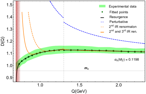
Our strategy is to find both the overall normalization of the large order expression , the non-perturbative constant , and by fitting the “experimental” values of the Adler function using the Eqs. (11) and (12). We show our main result in Fig. 1: the red shaded area indicates the energy region where the coupling approaches the Landau pole. The dashed orange line is the contribution assuming the IR renormalon at dominates the large order behavior; the solid orange line shows the improvement including also the IR renormalon at (we name the associated ambiguity as , consistent with the parametrization in Eq. (8)). Finally, the black line is our new result using the RRGE.
As can be seen from Fig. 1, the approximations with one and two IR renormalons drastically improve the perturbative result but they fail below the threshold. Conversely, our improvement fits the experimental values of the Adler function in the range between GeV, up to the region in which the coupling approaches the Landau pole. For higher energy, the non-perturbative corrections are exponentially suppressed and perturbation theory is recovered. In particular, it is worth appreciating the difference between the resurgent result (black line) and the two renormalon case (solid orange line) because both require three unknown constants to be fitted ( and , respectively). Thus, since both examples have the same number of inputs, the comparison clearly illustrates our improvement. The value for the , and from our fit are given by
| (13) |
The different values of and at the charm quark mass are due to the discontinuous change in the number of active flavors when the energy reach GeV. For completeness, when only the renormalon at (dashed orange line) is considered for and for . When only the first two renormalons at and are considered (solid orange line) for and for .
Remarks.
Let us discuss now possible issues and interpretations of our result within the RRGE.
-
•
Our approach requires the presence of the first IR renormalon because the structure of the Borel transform of Eq. (4) is characterized by poles at , being an integer between [28]. In particular, since the renormalon diagrams [44] gives quadratic poles, the Borel transform of the Adler function should be of the form
(14) However, the first IR renormalon at does not appear in the explicit calculation of the renormalon diagrams [5, 44], i.e. . This is the well-known first renormalon puzzle. As argued in Ref. [47], its presence must be related to UV effects and would then justify why it is not found in the IR expansion done in Ref. [44]. Furthermore, the explicit computation of Ref. [44] gives as well. We argue that the absence of is due to the incompleteness of the computation of Ref. [44] since it was done in the large (number of fermions) limit and does not include the gauge boson contributions. In conclusion and following well-known results, we have set in the resummation of the Adler function.
-
•
The Borel transform of Eq. (4) has poles at , which turn out to be quadratic for the specific case considered in this work. However, notice the coefficient receives a contribution proportional to [28] (see also below Eq. (4)), in agreement with the known renormalon structure [14, 48]. This leads to the appearance of multiple non-perturbative sectors corresponding to higher powers of in Eq. (11). These higher order terms are expected to be subleading in the energy range under consideration – below corrections to the leading result. Three and higher loop terms of the beta function do not enter in the transseries (11) since, as emphasized in Refs. [27, 28], only and are relevant for Eq. (4), making the transseries of Eq. (11) scheme-independent.
4 Summary
In this work, we propose a renormalon-based approximation of the QCD Adler function using a Borel-Ecalle resummation procedure. We provide an improvement to perturbation theory and as a result, we get a function that accurately follows the behavior of the data up to the Landau pole energy scale GeV. Around this scale, the coupling diverges and the transseries expansion ceases to work. In contrast to the operator-product-expansion, there are three unknown constants within this new approach, whereby the model is predictive. Notice that in this sense, it could have been wrong (which by itself is an achievement) and in fact, it starts failing outside the energy region of applicability. Finally, since we have fixed the constant in the transseries expansion of the Adler function in Eq. (11), the corrections to the heavy quark masses of Refs. [38, 39] can be unambiguously computed. It might also be interesting to merge our approach with the analytic one of Refs. [10, 11, 12]. These issues are left for future work.
Acknowledgement
AM was partially supported by the Croatian Science Foundation project number 4418. JCV was supported in part under the U.S. Department of Energy contract DE-SC0015376.
References and Notes
- [1] D. J. Gross and F. Wilczek, Ultraviolet behavior of non-abelian gauge theories, Phys. Rev. Lett. 30 (Jun, 1973) 1343–1346.
- [2] H. D. Politzer, Reliable perturbative results for strong interactions?, Phys. Rev. Lett. 30 (Jun, 1973) 1346–1349.
- [3] D. J. Gross and A. Neveu, Dynamical symmetry breaking in asymptotically free field theories, Phys. Rev. D 10 (Nov, 1974) 3235–3253.
- [4] B. Lautrup, On high order estimates in qed, Physics Letters B 69 (1977) 109–111.
- [5] G. ’t Hooft, Can We Make Sense Out of Quantum Chromodynamics?, Subnucl. Ser. 15 (1979) 943.
- [6] S. L. Adler, Some simple vacuum-polarization phenomenology: ; the muonic-atom x-ray discrepancy and , Phys. Rev. D 10 (Dec, 1974) 3714–3728.
- [7] S. Eidelman and F. Jegerlehner, Hadronic contributions to g-2 of the leptons and to the effective fine structure constant alpha (M(z)**2), Z. Phys. C 67 (1995) 585–602, [hep-ph/9502298].
- [8] S. Eidelman, F. Jegerlehner, A. L. Kataev and O. Veretin, Testing nonperturbative strong interaction effects via the Adler function, Phys. Lett. B 454 (1999) 369–380, [hep-ph/9812521].
- [9] A. Pich, Precision physics with inclusive QCD processes, Prog. Part. Nucl. Phys. 117 (2021) 103846, [2012.04716].
- [10] D. V. Shirkov and I. L. Solovtsov, Analytic model for the QCD running coupling with universal alpha-s (0) value, Phys. Rev. Lett. 79 (1997) 1209–1212, [hep-ph/9704333].
- [11] A. V. Nesterenko, Adler function in the analytic approach to QCD, eConf C0706044 (2007) 25, [0710.5878].
- [12] G. Cvetic and C. Valenzuela, Analytic QCD: A Short review, Braz. J. Phys. 38 (2008) 371–380, [0804.0872].
- [13] K. G. Wilson and W. Zimmermann, Operator product expansions and composite field operators in the general framework of quantum field theory, Comm. Math. Phys. 24 (1972) 87–106.
- [14] G. Parisi, The Borel Transform and the Renormalization Group, Phys. Rept. 49 (1979) 215–219.
- [15] M. Beneke, Renormalons, Phys. Rept. 317 (1999) 1–142, [hep-ph/9807443].
- [16] G. Cvetič, Renormalon-motivated evaluation of QCD observables, Phys. Rev. D 99 (2019) 014028, [1812.01580].
- [17] J. Écalle, Six lectures on transseries, analysable functions and the constructive proof of dulac’s conjecture, .
- [18] G. V. Dunne and M. Unsal, Resurgence and Trans-series in Quantum Field Theory: The CP(N-1) Model, JHEP 11 (2012) 170, [1210.2423].
- [19] P. J. Clavier, Borel-Ecalle resummation of a two-point function, 1912.03237.
- [20] M. Borinsky and G. V. Dunne, Non-Perturbative Completion of Hopf-Algebraic Dyson-Schwinger Equations, Nucl. Phys. B 957 (2020) 115096, [2005.04265].
- [21] T. Fujimori, M. Honda, S. Kamata, T. Misumi, N. Sakai and T. Yoda, Quantum phase transition and Resurgence: Lessons from 3d SQED, 2103.13654.
- [22] O. Costin and G. V. Dunne, Resurgent extrapolation: rebuilding a function from asymptotic data. Painlevé I, J. Phys. A 52 (2019) 445205, [1904.11593].
- [23] O. Costin and G. V. Dunne, Physical Resurgent Extrapolation, Phys. Lett. B 808 (2020) 135627, [2003.07451].
- [24] A. Maiezza and J. C. Vasquez, Renormalons in a general Quantum Field Theory, Annals Phys. 394 (2018) 84–97, [1802.06022].
- [25] E. Cavalcanti, Renormalons beyond the Borel plane, Phys. Rev. D 103 (2021) 025019, [2011.11175].
- [26] A. A. Mahmoud and K. Yeats, Connected Chord Diagrams and the Combinatorics of Asymptotic Expansions, 2010.06550.
- [27] A. Maiezza and J. C. Vasquez, Non-local Lagrangians from Renormalons and Analyzable Functions, Annals Phys. 407 (2019) 78–91, [1902.05847].
- [28] J. Bersini, A. Maiezza and J. C. Vasquez, Resurgence of the Renormalization Group Equation, Annals Phys. 415 (2020) 168126, [1910.14507].
- [29] O. CostinInternational Mathematics Research Notices 1995 (1995) 377.
- [30] O. Costin, Asymptotics and Borel Summability. Monographs and Surveys in Pure and Applied Mathematics. Chapman and Hall/CRC (2008), .
- [31] A. Maiezza and J. C. Vasquez, Non-Wilsonian ultraviolet completion via transseries, Int. J. Mod. Phys. A 36 (2021) 2150016, [2007.01270].
- [32] A. Maiezza and J. C. Vasquez, On Haag’s theorem and renormalization ambiguities, 2011.08875.
- [33] B. G. Weeks, The Apparent Double Valuedness of the Electric Charge in QED, .
- [34] M. Beneke and S. Jager, Spectator scattering at NLO in non-leptonic B decays: Leading penguin amplitudes, Nucl. Phys. B 768 (2007) 51–84, [hep-ph/0610322].
- [35] J. C. Collins, A. V. Manohar and M. B. Wise, Renormalization of the vector current in QED, Phys. Rev. D 73 (2006) 105019, [hep-th/0512187].
- [36] E. De Rafael and J. Rosner, Short-distance behavior of quantum electrodynamics and the callan-symanzik equation for the photon propagator, Annals Phys. 82 (1974) 369–406.
- [37] D. J. Broadhurst, Large N expansion of QED: Asymptotic photon propagator and contributions to the muon anomaly, for any number of loops, Z. Phys. C 58 (1993) 339–346.
- [38] I. I. Y. Bigi, M. A. Shifman, N. G. Uraltsev and A. I. Vainshtein, The Pole mass of the heavy quark. Perturbation theory and beyond, Phys. Rev. D 50 (1994) 2234–2246, [hep-ph/9402360].
- [39] M. Beneke and V. M. Braun, Heavy quark effective theory beyond perturbation theory: Renormalons, the pole mass and the residual mass term, Nucl. Phys. B 426 (1994) 301–343, [hep-ph/9402364].
- [40] D. Dorigoni, An Introduction to Resurgence, Trans-Series and Alien Calculus, Annals Phys. 409 (2019) 167914, [1411.3585].
- [41] S. G. Gorishnii, A. L. Kataev and S. A. Larin, The -corrections to and in QCD, Phys. Lett. B 259 (1991) 144–150.
- [42] L. R. Surguladze and M. A. Samuel, Total hadronic cross-section in e+ e- annihilation at the four loop level of perturbative QCD, Phys. Rev. Lett. 66 (1991) 560–563.
- [43] A. L. Kataev and V. V. Starshenko, Estimates of the higher order QCD corrections to R(s), R(tau) and deep inelastic scattering sum rules, Mod. Phys. Lett. A 10 (1995) 235–250, [hep-ph/9502348].
- [44] M. Neubert, Scale setting in QCD and the momentum flow in Feynman diagrams, Phys. Rev. D 51 (1995) 5924–5941, [hep-ph/9412265].
- [45] I. Caprini, Conformal mapping of the Borel plane: going beyond perturbative QCD, Phys. Rev. D 102 (2020) 054017, [2006.16605].
- [46] Particle Data Group collaboration, P. A. Zyla et al., Review of Particle Physics, PTEP 2020 (2020) 083C01.
- [47] V. I. Zakharov, Renormalons as a Bridge between Perturbative and Non-Perturbative Physics, Progress of Theoretical Physics Supplement 131 (02, 1998) 107–127, [https://academic.oup.com/ptps/article-pdf/doi/10.1143/PTPS.131.107/5430861/131-107.pdf].
- [48] E. Gardi and G. Grunberg, Conformal expansions and renormalons, Phys. Lett. B 517 (2001) 215–221, [hep-ph/0107300].