Co-clustering of time-dependent data
via Shape Invariant Model

Abstract

Multivariate time-dependent data, where multiple features are observed over time for a set of individuals, are increasingly widespread in many application domains. To model these data we need to account for relations among both time instants and variables and, at the same time, for subjects heterogeneity. We propose a new co-clustering methodology for clustering individuals and variables simultaneously that is designed to handle both functional and longitudinal data. Our approach borrows some concepts from the curve registration framework by embedding the Shape Invariant Model in the Latent Block Model, estimated via a suitable modification of the SEM-Gibbs algorithm. The resulting procedure allows for several user-defined specifications of the notion of cluster that could be chosen on substantive grounds and provides parsimonious summaries of complex longitudinal or functional data by partitioning data matrices into homogeneous blocks.

Keywords: co-clustering, curve registration, latent block model, stochastic EM

1 Introduction

Time dependent data, arising when measurements are taken on a set of units at different time occasions, are pervasive in a plethora of different fields. Examples include, but are not limited to, time evolution of asset prices and volatility in finance, growth of countries as measured by economic indices, heart or brain activities as monitored by medical instruments, disease evolution evaluated by suitable bio-markers in epidemiology. When analyzing such data, we need strategies modelling typical time courses by accounting for the individual correlation over time. In fact, while nomenclature and taxonomy in this setting are not always consistent, we might highlight some relevant differences, subsequently implying different challenges in the modelling process, in time-dependent data structures. On opposite poles, we may distinguish functional from longitudinal data analysis. In the former case the quantity of interest is supposed to vary over a continuum and usually a large number of regularly sampled observations is available, allowing to treat each element of the sample as a function. On the other hand, in longitudinal studies, time observations are often shorter with sparse and irregular measurements. Readers may refer to Rice (2004) for a thorough comparison and discussion about differences and similarities between functional and longitudinal data analysis.

Early development in these areas mainly aimed to describe individual-specific curves by properly accounting for the correlation between measurements for each subject (see e.g. Diggle et al., 2002; Ramsay and Silverman, 2005, and references therein) with the subjects themselves often considered to be independent. Nonetheless this is not always the case. Therefore, more recently, there has been an increased attention towards clustering methodologies aimed at describing heterogeneity among time-dependent observed trajectories; see Erosheva et al. (2014) for a recent review of related methods used in criminology and developmental psychology. From a functional standpoint, different approaches have been studied and readers may refer to the works by Bouveyron and Jacques (2011), Bouveyron et al. (2015) and Bouveyron et al. (2020) or to Jacques and Preda (2014) for a review. On the other hand, from a longitudinal point of view, model-based clustering approaches have been proposed by De la Cruz-Mesía et al. (2008), McNicholas and Murphy (2010). Lastly a review from a more general time-series data perspective may be found in Liao (2005) and Frühwirth-Schnatter (2011).

The methods cited so far usually deal with situations where a single feature is measured over time for a number of subjects, where therefore the data are represented by a $n\times T$ matrix, with $n$ and $T$ being the number of subjects and of observed time occasions. Nonetheless it is increasingly common to encounter multivariate time-dependent data, where several variables are measured over time for different individuals. These data may be represented according to three-way $n\times d\times T$ matrices, with $d$ being the number of time-dependent features; a graphical illustration of such structure is displayed in Figure 1. The introduction of an additional layer entails new challenges that have to be faced by clustering tools. In fact, as noted by Anderlucci and Viroli (2015), models have to account for three different aspects, being the correlation across different time observations, the relationships between the variables and the heterogeneity among the units, each one of them arising from a different layer of the three-way data structure.

Figure 1: Example of multivariate time-dependent data: $d=4$ variables are measured for $n=8$ individuals over $T=15$ time instants, giving rise to the displayed curves.

To extract useful information and unveil patterns from such complex structured and high-dimensional data, standard clustering strategies would require specification and estimation of severely parameterized models. In this situation, parsimony has often been induced by somehow neglecting the correlation structure among variables. A possible clever workaround, specifically proposed in a parametric setting, is represented by the contributions of Viroli (2011a, b) where, in order to handle three-way data, mixtures of Gaussian matrix-variate distributions are exploited.

In the present work, a different direction is taken, and a co-clustering strategy is pursued to address the mentioned issues. The term co-clustering refers to those methods aimed to find simultaneously row and column clusters of a data matrix. These techniques are particularly useful in high-dimensional settings where standard clustering methods may fall short in uncovering meaningful and interpretable row groups because of the high number of variables. By searching for homogeneous blocks in large matrices, co-clustering tools provide parsimonious summaries possibly useful both as dimensionality reduction and as exploratory steps. These techniques are particularly appropriate when relations among the observed variables are of interest. Note that, even in the co-clustering context, the usual dualism between distance-based and density-based strategies can be found. We pursue the latter approach which embeds co-clustering in probabilistic framework, builds a common framework to handle different types of data and reflects the idea of a density resulting from a mixture model. Specifically, we propose a parametric model for time-dependent data and a new estimation strategy to handle the distinctive characteristics of the model. Parametric co-clustering of time-dependent data has been pursued by Ben Slimen et al. (2018) and Bouveyron et al. (2018) in the functional setting, by mapping the original curves to the space spanned by the coefficients of a basis expansion. Unlike these contributions, we build on the idea that individual curves within a cluster arise as transformations of a common shape function which is modeled in such a way as to handle both functional and longitudinal data. Our co-clustering framework allows for easy interpretation and cluster description but also for specification of different notions of clusters which, depending on subject matter application, may be more desirable and interpretable by subject matter experts.

The rest of the paper is organized as follows. In Section 2, we provide the background needed for the specification of the proposed model which is described in Section 3, along with the estimation procedure. In Section 4, the model performances are illustrated both on simulated and real examples. We conclude the paper by summarizing our contributions and pointing to some future research directions.

2 Modelling time-dependent data

When dealing with the heterogeneous time dependent data landscape, outlined in the previous section, a variety of modelling approaches are sensible to be pursued. The route we follow in this work borrows its rationale from the curve registration framework (Ramsay and Li, 1998), according to which observed curves often exhibit common patterns but with some variations. Methods for curve registration, also known as curve alignment or time warping, are based on the idea of aligning prominent features in a set of curves via either an amplitude variation, a phase variation or a combination of the two. The first one is concerned with vertical variations while the latter regards horizontal, hence time related, ones. As an example it is possible to think about modelling the evolution of a specific disease. Here the observable heterogeneity of the raw curves can often be disentangled in two distinct sources: on the one hand, it could depend on differences in the intensities of the disease among subjects whereas, on the other hand, there could be different ages of onset, i.e. the age at which an individual experiences the first symptoms. After properly taking into account these causes of variation, the curves result to be more homogeneously behaving, with a so called warping function, which synchronizes the observed curves and allows for visualization and estimation of a common mean shape curve.

Coherently with the aforementioned rationale, in this work time dependency is accounted for via a self-modelling regression approach (Lawton et al., 1972) and, more specifically, via an extension to the so called Shape Invariant Model (SIM, Lindstrom, 1995), based on the idea that an individual curve arises as a simple transformation of a common shape function.
Let $\mathcal{X}=\{x_{i}({\bf t_{i}})\}_{1\leq i\leq n}$ be the set of curves, observed on $n$ individuals, with $x_{i}(t)$ being the level of the i-th curve at time $t$ and $t\in{\bf t_{i}}=(t_{1},\dots,T_{n_{i}})$, hence with the number of observed measurements allowed to be subject-specific. Stemming from the SIM, $x_{i}(t)$ is modelled as

$$x_{i}(t)=\alpha_{i,1}+\text{e}^{\alpha_{i,2}}m(t-\alpha_{i,3})+\epsilon_{i}(t)\;$$ (1)

where

• $m(\cdot)$ denotes a general common shape function whose specification is arbitrary. In the following we consider B-spline basis functions (De Boor, 1978), i.e. giving $m(t)=m(t;\beta)=\mathcal{B}(t)\beta,$ where $\mathcal{B}(t)$ and $\beta$ are respectively a vector of B-spline basis evaluated at time $t$ and a vector of basis coefficients whose dimensions allow for different degrees of flexibility;

• $\alpha_{i}=(\alpha_{i,1},\alpha_{i,2},\alpha_{i,3})\sim\mathcal{N}_{3}(\mu^{\alpha},\Sigma^{\alpha})$ for $i=1,\dots,n$ is a vector of subject-specific normally distributed random effects. These random effects are responsible for the individual specific transformations of the mean shape curve $m(\cdot)$ assumed to generate the observed ones. In particular $\alpha_{i,1}$ and $\alpha_{i,3}$ govern respectively amplitude and phase variations while $\alpha_{i,2}$ describes possible scale transformations. Random effects also allow accounting for the correlation among observations on the same subject measured at different time points. Following Lindstrom (1995), the parameter $\alpha_{i,2}$ is here optimized in the log-scale to avoid identifiability issues;

• $\epsilon_{i}(t)\sim\mathcal{N}(0,\sigma^{2}_{\epsilon})$ is a Gaussian distributed error term.

Due to its flexibility, the SIM has already been considered as a stepping stone to model functional as well as longitudinal time-dependent data (Telesca and Inoue, 2008; Telesca et al., 2012). Indeed, on the one hand, the smoothing involved in the specification of $m(\cdot;\beta)$ allows to handle function-like data. On the other hand, random effects, which borrow information across curves, make this approach fruitful even with short, irregular and sparsely sampled time series; readers may refer to Erosheva et al. (2014) for an illustration of this capabilities in the context of behavioral trajectories. Therefore, we find model (1) particularly appealing and suitable for our aims, potentially able to handle time-dependent data in a comprehensive way.

3 Time-dependent Latent Block Model

3.1 Latent Block Model

In the parametric, or model-based, co-clustering framework, the Latent Block Model (LBM, Govaert and Nadif, 2013) is the most popular approach. Data are represented in a matrix form $\mathcal{X}=\{x_{ij}\}_{1\leq i\leq n,1\leq j\leq d}$, where by now we should intend $x_{ij}$ as a generic random variable. To aid the definition of the model, and in accordance with the parametric approach to clustering (Fraley and Raftery, 2002; Bouveyron et al., 2019), two latent random vectors $\mathbf{z}=\{z_{i}\}_{1\leq i\leq n}$, and $\mathbf{w}=\{w_{j}\}_{1\leq j\leq d}$, with $z_{i}=(z_{i1},\dots,z_{iK})$, $w_{j}=(w_{j1},\dots,w_{jL})$, are introduced, indicating respectively the row and column memberships, with $K$ and $L$ the number of row and column clusters. A standard binary notation is used for the latent variables, i.e. $z_{ik}=1$ if the i-th observation belongs to the k-th row cluster and 0 otherwise and, likewise, $w_{jl}=1$ if the j-th variable belongs to the l-th column cluster and 0 otherwise. The model formulation relies on a local independence assumption, i.e. the $n\times d$ random variables $\{x_{ij}\}_{1\leq i\leq n,1\leq j\leq d}$ are assumed to be independent conditionally on $\mathbf{z}$ and $\mathbf{w},$ in turn supposed to be independent. The LBM can be thus written as

$$p(\mathcal{X};\Theta)=\sum_{z\in Z}\sum_{w\in W}p(\mathbf{z};\Theta)p(\mathbf{w};\Theta)p(\mathcal{X}|\mathbf{z},\mathbf{w};\Theta)\;,$$ (2)

where

• $Z$ and $W$ are the sets of all the possible partitions of rows and columns respectively in $K$ and $L$ groups;

• the latent vectors $\mathbf{z},\mathbf{w}$ are assumed to be multinomial, with $p(\mathbf{z};\Theta)=\prod_{ik}\pi_{k}^{z_{ik}}$ and $p(\mathbf{w};\Theta)=\prod_{jl}\rho_{l}^{w_{jl}}$ where $\pi_{k},\rho_{l}>0$ are the row and column mixture proportions, $\sum_{k}\pi_{k}=\sum_{l}\rho_{l}=1$;

• as a consequence of the local independence assumption, $p(\mathcal{X}|\mathbf{z},\mathbf{w};\Theta)=\prod_{ijkl}p(x_{ij};\theta_{kl})^{z_{ik}w_{jl}}$ where $\theta_{kl}$ is the vector of parameters specific to block $(k,l)$;

• $\Theta=(\pi_{k},\rho_{l},\theta_{kl})_{1\leq k\leq K,1\leq l\leq L}$ is the full parameter vector of the model.

The LBM is particularly flexible in modelling different data types, as handled by a proper specification of the marginal density $p(x_{ij};\theta_{kl})$ for binary (Govaert and Nadif, 2003), count (Govaert and Nadif, 2010), continuous (Lomet, 2012), categorical (Keribin et al., 2015), ordinal (Jacques and Biernacki, 2018; Corneli et al., 2020), and even mixed-type data (Selosse et al., 2020).

3.2 Model specification

Once the LBM structure has been properly defined, extending its rationale to handle time-dependent data in a co-clustering framework boils down to a suitable specification of $p(x_{ij};\theta_{kl})$. Note that this reveals one of the main advantage of such an highly-structured model, consisting in the chance to search for patterns in multivariate and complex data by specifying only the model for the variable $x_{ij}$. As introduced in Section 1, multidimensional time-dependent data may be represented according to a three-way structure where the third mode accounts for the time evolution. The observed data assume an array configuration $\mathcal{X}=\{x_{ij}({\bf t_{i}})\}_{1\leq i\leq n,1\leq j\leq d}$ with ${\bf t_{i}}=(t_{1},\dots,T_{n_{i}})$ as outlined in Section 2; different observational lengths can be handled by a suitable use of missing entries. Consistently with (1), we consider as a generative model for the curve in the $(i,j)$-th entry, belonging to the generic block $(k,l)$, the following

$$x_{ij}(t)|_{z_{ik}=1,w_{jl}=1}=\alpha_{ij,1}^{kl}+\text{e}^{\alpha_{ij,2}^{kl}}m(t-\alpha_{ij,3}^{kl};\beta_{kl})+\epsilon_{ij}(t)\;$$ (3)

with $t\in{\bf t_{i}}$ a generic time instant. A relevant difference with respect to the original SIM consists, coherently with the co-clustering setting, in the parameters being block-specific since the generative model is specified conditionally to the block membership of the cell. As a consequence:

• $m(t;\beta_{kl})=\mathcal{B}(t)\beta_{kl}$ where the quantities are defined as in Section 2, with the only difference that $\beta_{kl}$ is a vector of block-specific basis coefficients, hence allowing different mean shape curves across different blocks;

• $\alpha_{ij}^{kl}=(\alpha_{ij,1}^{kl},\alpha_{ij,2}^{kl},\alpha_{ij,3}^{kl})\sim\mathcal{N}_{3}(\mu_{kl}^{\alpha},\Sigma_{kl}^{\alpha})$ is a vector of cell-specific random effects distributed according to a block-specific Gaussian distribution;

• $\epsilon_{ij}(t)\sim\mathcal{N}(0,\sigma^{2}_{\epsilon,kl})$ is the error term distributed as a block-specific Gaussian;

• $\theta_{kl}=(\mu_{kl}^{\alpha},\Sigma_{kl}^{\alpha},\sigma^{2}_{\epsilon,kl},\beta_{kl})$.

Note that the ideas borrowed from the curve registration framework are here embedded in a clustering setting. Therefore, while curve alignment aims to synchronize the curves to estimate a common mean shape, in our setting the SIM works as a suitable tool to model the heterogeneity inside a block and to introduce a flexible notion of cluster. The rationale behind considering the SIM in a co-clustering framework consists in looking for blocks characterized by a different mean shape function $m(\cdot;\beta_{kl})$. Curves within the same block arise as random shifts and scale transformations of $m(\cdot;\beta_{kl}),$ driven by the block-specifically distributed random effects. Let consider the small panels on the left side of Figure 2, displaying a number of curves which arise as transformations induced by non-zero values of $\alpha_{ij,1},$ $\alpha_{ij,2},$ or $\alpha_{ij,3}$. Beyond the sample variability, the curves differ for a (phase) random shift on the $x-$axes, an amplitude shift on the $y-$ axes, and a scale factor. According to model (3), all those curves belong to the same cluster, since they share the same mean shape function (Figure 2, right panel).

Figure 2: In the left panels, curves in dotted line arise as random fluctuations of the superimposed red curve, but they are all time, amplitude or scale transformations of the same mean-shape function on the right panel.

In fact, further flexibility can be naturally introduced within the model by “switching off” one or more random effects, depending on subject-matter considerations and on the concept of cluster one has in mind. If there are reasons to support that similar time evolutions associated to different intensities are, in fact, expression of different clusters, it makes sense to switch off the random intercept $\alpha_{ij,1}$. In the example illustrated in Figure 2 this ideally leads to a two-clusters structure (Figure 3, left panels). Similarly, switching off the random effect $\alpha_{ij,3}$ would lead to blocks characterized by a shifted time evolution (Figure 3, right panels), while removing $\alpha_{ij,2}$ determines different blocks varying for a scale factor (Figure 3, middle panels).

FTT

TFT

TTF

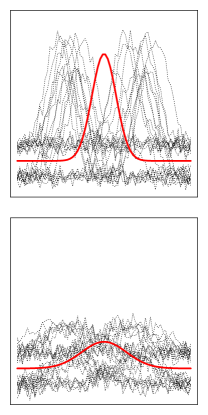
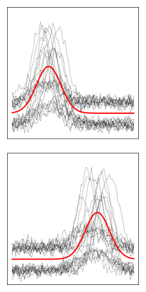
Figure 3: Pairs of plots in each column represent the two-cluster configurations arising from switching off, from left to right $\alpha_{ij,1}$, $\alpha_{ij,2},$ $\alpha_{ij,3}$. In the names of the models, as used in the rest of the paper, T indicates a switched on random effect while F a switched off one.

3.3 Model estimation

To estimate the LBM several approaches have been proposed, as for example Bayesian (Wyse and Friel, 2012), greedy search (Wyse et al., 2017) and likelihood-based ones (Govaert and Nadif, 2008). In this work we focus on the latter class of methods. In principle, the estimation strategy would aim to maximize the log-likelihood $\ell(\Theta)=\log p(\mathcal{X};\Theta)$ with $p(\mathcal{X};\theta)$ defined as in (2); nonetheless, the missing structure of the data makes this maximization impractical. For this reason the complete data log-likelihood is usually considered as the objective function to optimize, being defined as

$$\ell_{c}(\Theta,\mathbf{z},\mathbf{w})=\sum_{ik}z_{ik}\log\pi_{k}+\sum_{jl}w_{jl}\log\rho_{l}+\sum_{ijkl}z_{ik}w_{jl}\log p(x_{ij};\theta_{kl})$$ (4)

where the first two terms account for the proportions of row and column clusters while the third one depends on the probability density function of each block.

As a general solution, to maximize (4) and obtain an estimate of $\hat{\Theta}$ when dealing with situations where latent variables are involved, one would instinctively resort to the Expectation-Maximization algorithm (EM, Dempster et al., 1977). The basic idea underlying the EM algorithm consists in finding a lower bound of the log-likelihood and optimizing it via an iterative scheme in order to create a converging series of $\hat{\Theta}^{(h)}$ (see Wu, 1983, for more details about the convergence properties of the algorithm). In the co-clustering framework, this lower bound can be easily exhibited by rewriting the log-likelihood as follows

$$\ell(\Theta)=\mathcal{L}(q;\Theta)+\zeta$$

where $\mathcal{L}(q;\Theta)=\sum_{{\bf z},{\bf w}}q({\bf z},{\bf w})\log(p(\mathcal{X},{\bf z},{\bf w}|\theta)/q({\bf z},{\bf w}))$ with $q({\bf z},{\bf w})$ being a generic probability mass function on the support of $({\bf z},{\bf w})$ while $\zeta$ is a positive constant not depending on $\Theta$.

The E step of the algorithm maximizes the lower bound $\mathcal{L}$ over $q$ for a given value of $\Theta$. Straightforward calculations show that $\mathcal{L}$ is maximized for $q^{*}({\bf z},{\bf w})=p({\bf z},{\bf w}|\mathcal{X},\theta)$. Unfortunately, in a co-clustering scenario, the joint posterior distribution $p({\bf z},{\bf w}|\mathcal{X},\Theta)$ is not tractable, as it involves terms that cannot be factorized as it conversely happens in a standard mixture model framework. As a consequence, several modifications have been explored, searching for viable solutions when performing the E step (see Govaert and Nadif, 2013, for a more detailed tractation); examples are the Classification EM (CEM) and the Variational EM (VEM). Here we propose to make use of a Gibbs sampler within the E step to approximate the posterior distribution $p({\bf z},{\bf w}|\mathcal{X},\Theta)$. This results in a stochastic version of the EM algorithm, which will be called SEM-Gibbs in the following. Given an initial column partition ${\bf w^{(0)}}$ and an initial value for the parameters $\Theta^{(0)}$, at the $h$-th iteration the algorithm proceeds as follows

• SE step: $q^{*}({\bf z},{\bf w})\simeq p({\bf z},{\bf w}|\mathcal{X},\Theta^{(h-1)})$ is approximated with a Gibbs sampler. The Gibbs sampler consists in sampling alternatively ${\bf z}$ and ${\bf w}$ from their conditional distributions a certain number of times before to retain new values for ${\bf z}^{(h)}$ and ${\bf w}^{(h)}$,

• M step: $\mathcal{L}(q^{*}({\bf z},{\bf w}),\Theta^{(h-1)})$ is then maximized over $\Theta$, where

  $$\mathcal{L}(q^{*}({\bf z},{\bf w}),\Theta^{(h-1)}) \simeq\sum_{z,w}p({\bf z},{\bf w}|\mathcal{X},\Theta^{(h-1)})\log(p(\mathcal{X},{\bf z},{\bf w}|\Theta)/p({\bf z},{\bf w}|\mathcal{X},\Theta^{(h-1)}))$$

  $$\simeq E[\ell_{c}(\Theta,{\bf z}^{(h)},{\bf w}^{(h)})|\Theta^{(h-1)}]+\xi,$$

  $\xi$ not depending on $\Theta$. This step therefore reduces to the maximization of the conditional expectation of the complete data log-likelihood (4) given $\bf{z}^{(h)}$ and ${\bf w}^{(h)}$.

In the proposed framework, due to the presence of the random effects, some additional challenges have to be faced. In fact, the maximization of the conditional expectation of (4) associated to model (3) requires a cumbersome multidimensional integration in order to compute the marginal density defined as

$$p(x_{ij};\theta_{kl})=\int p(x_{ij}|\alpha_{ij}^{kl};\theta_{kl})p(\alpha_{ij}^{kl};\theta_{kl})\,d\alpha_{ij}^{kl}\;.$$ (5)

Note that, with a slight abuse of notation, we suppress here the dependency on the time $t$, i.e. $x_{ij}$ has to be intended as $x_{ij}({\bf t_{i}})$. In the SE step, on the other hand, the evaluation of (5) is needed for all the possible configurations of $\{z_{i}\}_{i=1,\dots,n}$ and $\{w_{j}\}_{j=1,\dots,d}$. These quantities are straightforwardly obtained when considering the SEM-Gibbs to estimate models without any random effect involved, while their computation is more troublesome in our scenario.

For these reasons, we propose a modification of the SEM-Gibbs algorithm, called Marginalized SEM-Gibbs (M-SEM), where an additional Marginalization step is introduced to properly account for the random effects. Given an initial value for the parameters $\Theta^{(0)}$ and an initial column partition $\mathbf{w}^{(0)}$, the $h$-th iteration of the M-SEM algorithm alternates the following steps:

• Marginalization step: The single cell contributions in (5) to the complete data log-likelihood are computed by means of a Monte Carlo integration scheme as follows

  $$p(x_{ij};\theta_{kl}^{(q)})\simeq\frac{1}{M}\sum_{m=1}^{M}p(x_{ij};\alpha_{ij}^{kl,(m)},\theta_{kl}^{(h-1)})\;$$ (6)

  for $i=1,\dots,n$, $j=1,\dots,d$, $k=1,\dots,K$ and $l=1,\dots,L$ and being $M$ the number of Monte Carlo samples. The values of the vectors $\alpha_{ij}^{kl,(1)},\dots,\alpha_{ij}^{kl,(M)}$ are drawn from a Gaussian distribution $\mathcal{N}_{3}(\mu_{kl}^{\alpha,(h-1)},\Sigma_{kl}^{\alpha,(h-1)})$; note that this choice amounts to a random version of the Gaussian quadrature rule (see e.g. Pinheiro and Bates, 2006);

• SE step: $p({\bf z},{\bf w}|\mathcal{X},\Theta^{(h-1)})$ is approximated by repeating, for a number of iterations, the following Gibbs sampling steps

  1. generate the row partition $z_{i}^{(h)}=(z_{i1}^{(h)},\dots,z_{iK}^{(h)}),\;i=1,\dots,n$ according to a multinomial distribution $z_{i}^{(h)}\sim\mathcal{M}(1,\tilde{z}_{i1},\dots,\tilde{z}_{iK})$, with

     $$\tilde{z}_{ik} = p(z_{ik}=1|\mathcal{X},\mathbf{w}^{(h-1)};\Theta^{(h-1)})$$

     $$= \frac{\pi_{k}^{(h-1)}p_{k}(\mathbf{x}_{i}|\*w^{(h-1)};\Theta^{(h-1)})}{\sum_{k^{\prime}}\pi_{k^{\prime}}^{(h-1)}p_{k^{\prime}}(\mathbf{x}_{i}|\*w^{(h-1)};\Theta^{(h-1)})}\;,$$

     for $k=1,\dots,K$, $\mathbf{x}_{i}=\{x_{ij}\}_{1\leq j\leq d}$ and $p_{k}(\mathbf{x}_{i}|\mathbf{w}^{(h-1)};\Theta^{(h-1)})=\prod_{jl}p(x_{ij};\theta_{kl}^{(h-1)})^{w_{jl}^{(h-1)}}$.

  2. generate the column partition $w_{j}^{(h)}=(w_{j1}^{(h)},\dots,w_{jL}^{(h)}),\;j=1,\dots,d$ according to a multinomial distribution $w_{j}^{(h)}\sim\mathcal{M}(1,\tilde{w}_{j1},\dots,\tilde{w}_{jL})$, with

     $$\tilde{w}_{jl} = p(w_{jl}=1|\mathcal{X},\mathbf{z}^{(h)};\Theta^{(h-1)})$$

     $$= \frac{\rho_{l}^{(q)}p_{l}(\mathbf{x}_{j}|\mathbf{z}^{(h)};\Theta^{(h-1)})}{\sum_{l^{\prime}}\rho_{l^{\prime}}^{(h-1)}p_{l^{\prime}}(\mathbf{x}_{j}|\mathbf{z}^{(h)};\Theta^{(h-1)})}\;,$$

     for $l=1,\dots,L$, $\mathbf{x}_{j}=\{x_{ij}\}_{1\leq i\leq n}$ and $p_{l}(\mathbf{x}_{j}|\mathbf{z}^{(h)};\Theta^{(h-1)})=\prod_{ik}p(x_{ij};\Theta_{kl}^{(h-1)})^{z_{ik}^{(h)}}$.

• M step: Estimate $\Theta^{(h)}$ by maximizing $E[\ell_{c}(\Theta,{\bf z}^{(h)},{\bf w}^{(h)})|\Theta^{(h-1)}]$.
  Mixture proportions are updated as $\pi_{k}^{(h)}=\frac{1}{n}\sum_{i}z_{ik}^{(h)}$ and $\rho_{l}^{(h)}=\frac{1}{d}\sum_{j}w_{jl}^{(h)}$. The estimate of $\theta_{kl}=(\mu_{kl}^{\alpha},\Sigma_{kl}^{\alpha},\sigma^{2}_{\epsilon,kl},\beta_{kl})$ is obtained by exploiting the non-linear mixed effect model specification in (3) and considering the approximate maximum likelihood formulation proposed in Lindstrom and Bates (1990); the variance and the mean components are estimated by approximating and maximizing the marginal density of the latter near the mode of the posterior distribution of the random effects. Conditional or shrinkage estimates are then used for the estimation of the random effects.

The M-SEM algorithm is run for a certain number of iterations until a convergence criterion on the complete data log-likelihood is met. Since a burn-in period is considered, the final estimate for $\Theta$, denoted as $\hat{\Theta}$, is given by the mean of the sample distribution. A sample of $(\mathbf{z},\mathbf{w})$ is then generated according to the SE step as illustrated above with $\Theta=\hat{\Theta}$. The final block-partition $(\hat{\mathbf{z}},\hat{\mathbf{w}})$ is then obtained as the mode of their sample distribution.

3.4 Model selection

The choice of the number of groups is considered here as a model selection problem. Operationally several models, corresponding to different combinations of $K$ and $L$ and, in our case, to different configurations of the random effects, are estimated and the best one is selected according to an information criterion. Note that the model selection step is more troublesome in this setting with respect to a standard clustering one, since we need to select not only the number of row clusters $K$ but also the number of column ones $L$. Standard choices, such as the AIC and the BIC, are not directly available in the co-clustering framework where, as noted by Keribin et al. (2015), the computation of the likelihood of the LBM is challenging, even when the parameters are properly estimated. Therefore, as a viable alternative, we consider an approximated version of the ICL (Biernacki et al., 2000) that, relying on the complete data log-likelihood, does not suffer from the same issues, and which reads as follows

$$\text{ICL}=\ell_{c}(\hat{\Theta},\hat{z},\hat{w})-\frac{K-1}{2}\log n-\frac{L-1}{2}\log d-\frac{KL\nu}{2}\log nd\;,$$ (7)

where $\nu$ denotes number of specific parameters for each block while $\ell_{c}(\hat{\Theta},\hat{z},\hat{w})$ is defined as in (4) with $\Theta$, $z$ and $w$ being replaced by their estimates. The model associated with the highest value of the ICL is then selected.

Even if the use of this criterion is a well-established practice in co-clustering applications, Keribin et al. (2015) noted that its consistency has not been proved yet to estimate the number of blocks of a LBM. Additionally, Nagin (2009) and Corneli and Erosheva (2020) point out a bias of the ICL towards overestimation of the number of clusters in the longitudinal context. The validity of the ICL could be additionally undermined by the presence of random effects. As noted by Delattre et al. (2014), standard information criteria have unclear definitions in a mixed effect model framework, since the definition of the actual sample size is not trivial. Given that, common asymptotic approximations are not valid anymore. Even if a proper exploration of the problem from a co-clustering perspective is still missing, we believe that the mentioned issues might have an impact also on the derivation of the criterion in (7). The development of valid model selection tools for LBM when random effects are involved is out of scope of this work, therefore, operationally, we consider the ICL. Nonetheless, the analyses in Section 4 have to be interpreted with full awareness of the limitations described above.

3.5 Remarks

The model introduced so far inherits the advantages of both the building ingredients, namely the LBM and the SIM, it embeds. Thanks to the local independence assumption of the LBM, it allows handling multivariate, possibly high-dimensional complex data structures in a relatively parsimonious way. Differences among the subjects are captured by the random effects, while curve summaries can be expressed as a functional of the mean shape curve. Additionally, resorting to a smoother when modeling the mean shape function, it allows for a flexible handling of functional data whereas the presence of random effects make the model effective also in a longitudinal setting. Finally, clustering is pursued directly on the observed curves, without resorting to intermediate transformation steps, as it is done in Bouveyron et al. (2018), where clustering is performed on the basis expansion coefficients used to transform the original data.

The attractive features of the model go hand in hand with some difficulties that require caution –namely, likelihood multimodality, the associated convergence issues, and the curse of flexibility– that we discuss below in turn.

• Initialization The M-SEM algorithm encloses different numerical steps which require the suitable specification of starting values. First, the convergence of EM-type algorithms towards a global maximum is not guaranteed; as a consequence they are known to be sensitive to the initialization with a proper one being crucial to avoid local solutions. Assuming $K$ and $L$ to be known, the M-SEM algorithm requires starting values for $\mathbf{z}$ and $\mathbf{w}$ in order to implement the first M step. A standard strategy resorts to multiple random initializations: the row and column partitions are sampled independently from multinomial distributions with uniform weights and the one eventually leading to the highest value of the complete data log-likelihood is retained. An alternative approach, possibly accelerating the convergence, is given by a k-means initialization, where two k-means algorithms are independently run for the rows and the columns of $\mathcal{X}$ and the M-SEM algorithm is initialized with the obtained partitions. It has been pointed out (see e.g. Govaert and Nadif, 2013) that the SEM-Gibbs, being a stochastic algorithm, can attenuate in practice the impact of the initialization on the resulting estimates. Finally, note that a further initialization is required, to estimate the nonlinear mean shape function within the M step.

• Convergence and other numerical problems. Although the benefits of including random effects in the considered framework are undeniable, parameters estimation is known not to be straightforward in mixed effect models, especially in the nonlinear setting (see, e.g. Harring and Liu, 2016). As noted above the nonlinear dependence of the conditional mean of the response on the random effects requires multidimensional integration to derive the marginal distribution of the data. While several methods have been proposed to compute the integral, convergence issues are often encountered. In such situations, some strategies can be employed to help with convergence of the estimation algorithm. Examples are to try different sets of starting values, to scale the data prior to the modeling step, or to simplify the structure of the model (e.g. by reducing the number of knots of the B-splines). Addressing these issues often results in considerable computational times even when convergence is eventually achieved. Depending on the specific data at hand, it is also possible to consider alternative mean shape formulations, such as polynomial functions, which result in easier estimation procedures. Lastly note that, if available, prior knowledge about the time evolution of the observed phenomenon may be incorporated in the models as it could introduce some constraints possibly simplifying the estimation process (see e.g. Telesca et al., 2012).

• Curse of flexibility. Including random effects for both phase and amplitude shifts and scale transformations might allow for a virtually excellent fitting of various arbitrarily shaped curve. This flexibility, albeit desirable, sometimes achieve excessive extents, possibly leading to estimation troubles. This is especially true in a clustering framework, where data are expected to exhibit a remarkable heterogeneity. From a practical point of view, our experience suggests that the estimation of the parameters $\alpha_{ij,2}$ turns out to be the most troublesome, sometimes leading to convergence issues and instability in the resulting estimates.

4 Numerical experiments

Before moving forward to the interest of the proposed approach on real-world situations, this section presents some numerical experiments illustrating its main features on simulated data.

4.1 Synthetic data

This section examines the main features of the proposed approach on some synthetic data. The aim of the simulation study is twofold. The first and primary goal of the analyses consists in exploring the capability of the proposed method to properly partition the data into blocks, also in comparison with some competitors such as the one proposed by Bouveyron et al. (2018) (funLBM in the following) and a double k-means approach, where row and column partitions are obtained separately and subsequently merged to produce blocks. As for the second aim of the simulations, we evaluate the performances of the ICL in the developed framework to select both the number $(K,L)$ of blocks and the random effect configuration.

All the analyes have been conducted in the R environment (R Core Team, 2019) with the aid of nlme package (Pinheiro et al., 2019), used to estimate the parameters in the M-step, and the splines package, used to handle the B-spline involved in the specification of the common shape function. The code implementing the proposed procedure is available upon request.

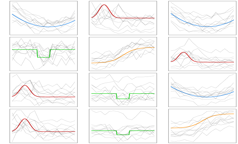
Figure 4: Subsample of simulated curves (black dashed lines) with over-imposed block specific mean shape curves (colored continue lines) employed in the numerical study

The examined simulation setup is defined as follows. We generated $B=100$ Monte Carlo samples of curves according to the general specification (3), with block-specific mean shape function $m_{kl}(\cdot)$ and both the parameters involved in the error term and the ones describing the random effects distribution being constant across the blocks. In fact, in the light of the considerations made in Section 3.5, the random scale parameter is switched off in the data generative mechanism, i.e. $\alpha_{ij,2}$ is constrained to be degenerate in zero. The number of row and column clusters has been fixed to $K_{\text{true}}=4$ and $L_{\text{true}}=3$. The mean shape functions $m_{kl}(\cdot)$ are chosen among four different curves, namely $m_{11}=m_{13}=m_{33}=m_{1}$, $m_{12}=m_{32}=m_{31}=m_{41}=m_{2}$, $m_{21}=m_{32}=m_{42}=m_{3}$ and $m_{22}=m_{43}=m_{4}$, as illustrated in Figure 4 with different color lines, and specified as follows:

$$m_{1}(t) \propto 6t^{2}-7t+1\hskip 85.35826ptm_{2}(t)\propto\phi(t;0.2,0.008)$$

$$m_{3}(t) \propto 0.75-0.8\mathbbm{1}_{\{t\in(0.4,0.6)\}}\hskip 39.83368ptm_{4}(t)\propto\frac{1}{(1+\exp(-10t+5))}$$

The other parameters involved have been set to $\sigma_{\epsilon,kl}=0.3$, $\mu_{kl}^{\alpha}=(0,0,0)$ and $\Sigma_{kl}^{\alpha}=\text{diag}(1,0,0.1)$ $\forall k=1,\dots,K_{\text{true}},l=1,\dots,L_{\text{true}}$. Three different scenarios are considered with generated curves consisting of $T=15$ equi-spaced observations ranging in $[0,1]$. As a first baseline scenario, we set the number of rows to $n=100$ and the number of columns to $d=20$. The other scenarios are considered in order to obtain insights and indications on the performances of the proposed method when dealing with larger matrices. Coherently in the second scenario $n=500$ and $d=20$ while in the third one $n=100$ and $d=50$ thus increasing respectively the number of samples and features.

As for the first goal of the simulation study, we explore the performances of our proposal in terms of the Co-clustering Adjusted Rand Index (CARI, Robert et al., 2020). This criterion generalizes the Adjusted Rand Index (Hubert and Arabie, 1985) to the co-clustering framework, and takes the value 1 when the blocks partitions perfectly agree up to a permutation. In order to have a fair comparison with the double k-means approach, for which selecting the number of blocks does not admit an obvious solution, and to separate the uncertainty due to model selection from the one due to cluster detection, models are compared by considering the number of blocks as known and equal to $(K_{\text{true}},L_{\text{true}})$. Consistently, we estimate our model only for the TFT random effects configuration, being the one generating the data. This is made possible by constraining mean and variance estimates of the scale-random effect to be equal to zero.

Results are reported in Table 1. The proposed method claims excellent performances in all the considered settings, with results notably featured by a very limited variability. No clear-cut indications arise from the comparison with funLBM as the two methodologies lead to comparable results. Conversely, the use of an approach which is not specifically conceived for co-clustering, like the the double k-means, leads to a strong degradation of the quality of the partitions. Unlike the results obtained with our method and with funLBM, being insensitive to changes in the dimensions of the data, the double k-means behaves better with an increased number of variables or observations.

Table 1: Mean (and std error) of the CARI computed over the simulated samples in the three scenarios. Partitions are obtained using the proposed approach (tdLBM), funLBM and a double k-means approach.

	$n=100,d=20$	$n=100,d=50$	$n=500,d=20$
CARI${}_{\text{{tdLBM}}}$	0.972 (0.044)	0.988 (0.051)	0.981 (0.020)
CARI${}_{\text{{funLBM}}}$	0.981 (0.066)	0.986 (0.053)	0.986 (0.060)
CARI${}_{\text{{kmeans}}}$	0.761 (0.158)	0.842 (0.182)	0.809 (0.169)

Table 2: Rate of selection of $(K,L)$ configurations for the different scenarios considered obtained using the proposed approach.

$n=100,d=20$	$n=100,d=50$	$n=500,d=20$

As for the performances of the ICL, Table 2 shows the fractions of samples where the criterion has led to the selection of each of the considered configurations of $(K,L)$, with $K,L=2,\dots,5$, for models estimated with the proposed method. In all the considered settings, the actual number of co-clusters is the most frequently selected by the ICL criterion. In fact, a non-negligible tendency to favor overparameterized models, especially for larger sample size, is witnessed, consistently with the comments in Corneli et al. (2020).

Similar considerations may be drawn from the exploration of the performances of the ICL when used to select the random effect configuration (Table 3). Here, the performances seem to be less influenced by the data dimensionality, and ICL selects the true configuration for the majority of the samples in two scenarios while, in the third one, the true model is selected approximately one out of two samples. Nonetheless, also in this case, a tendency to overestimation is visible, with the TTT configuration frequently selected in all the scenarios. In general, the penalization term in (7) seems to be too weak and overall not completely able to account for the presence of random effects. These results, along with the remarks at the end of Section 3.3, provide a suggestion about a possibly fruitful research direction which consists in proposing some suitable adjustments.

In fact, it is worth noting that when the selection of the number of clusters is the aim, the observed behavior is overall preferable with respect to underestimation since it does not undermine the homogeneity within a block, being the final aim of cluster analysis; this has been confirmed by further analyses suggesting that the additional groups are usually small and arising because of the presence of outliers. As for the random effect configuration, we believe that since the choice impacts the notion of cluster one aims to identify, it should be driven by subject-matter knowledge rather than by automatic criteria. Additionally, the reported analyses are exploratory in nature, aiming to provide general insights on the characteristics of the proposed approach. To limit computational time required to run the large number of models involved in Tables 2 and 3, for demonstration of our method, we did not use multiple initializations and we have pre-selected the number of knots for the block-specific mean functions. In practice, we recommend, at a minimum, using multiple starting values and carrying out sensitivity analyses on the number of knots to ensure that substantive conclusions are not affected.

Table 3: Rate of selection for each random effects configuration in the considered scenarios. T means that the corresponding random effect is switched on while F means that is switched off. As an example FTT represent a model where $\alpha_{ij,1}$ is constrained to be a random variable with degenerate distribution in zero. Bold cells represents the true data generative model (TFT), blank ones represent percentages equal to zero.

		FFF	TFF	FTF	FFT	TTF	TFT	FTT	TTT
	$n=100,d=20$					1%	58%		41%
% of selection	$n=100,d=50$		2%			1%	62%		35%
	$n=500,d=20$		1%			5%	47%		47%

4.2 Applications to real world problems

4.2.1 French Pollen Data

The data we consider in this section are provided by the Réseau National de Surveillance Aérobio-
logique (RNSA), the French institute which analyzes the biological particles content of the air and studies their impact on the human health. RNSA collects data on concentration of pollens and moulds in the air, along with some clinical data, in more than 70 municipalities in France.

The analyzed dataset contains daily observations of the concentration of 21 pollens for 71 cities in France in 2016. Concentration is measured as the number of pollens detected over a cubic meter of air and carried on by means of some pollen traps located in central urban positions over the roof of buildings, in order to be representative of the trend air quality.

The aim of the analysis is to identify homogeneous trends in the pollen concentration over the year and across different geographic areas. For this reason, we focus on finding groups of pollens differentiating one from the others for either the period of maximum exhibition or the time span they are present. Consistently with this choice, only models with the y-axis shift parameter $\alpha_{ij,1}$ are estimated (i.e. $\alpha_{ij,2}$ and $\alpha_{ij,3}$ are switched off), for varying number of row and column clusters, and the best one selected via ICL. We consider monthly data by averaging the observed daily concentrations over each month. The resulting dataset may be represented as a matrix with $n=71$ rows (cities), $p=21$ columns (pollens) where each entry is a sequence of $T=12$ time-indexed measurements. Moreover, to practically apply our proposed procedure on the data, a preprocessing step has been carried out. We work on a logarithmic scale and, in order to improve the stability of the estimation procedure, the data have been standardized.

Results are graphically displayed in Figure 5. The ICL selects a model with $K=3$ row clusters and $L=5$ column ones. A first visual inspection of the pollen time evolutions reveals that the procedure is able to discriminate the pollens according to their seasonality. Pollens in the first two column groups are mainly present during the summer, with a difference in the intensity of the concentration. In the remaining three groups pollens are more active, roughly speaking, during winter and spring months but with a different time persistence and evolution.

Digging deeper substantially in the cluster configuration obtained is beyond the scope of this work and may benefit from insights from experts of botanical and geographical disciplines. Anyway it stands out that column clusters are roughly grouping together trees pollens, distinguishing them from weed and grass ones (right panel of Table 4). Results align with the usually considered typical seasons, with groups of pollens from trees mostly present in winter and spring while the ones from grass spreading in the air mainly during the summer months. With respect to the row partition, displayed in the left panel of Table 4, three clusters have been detected, with one roughly corresponding to the Mediterranean region. The situation, for what it concerns the other two clusters, appears to be more heterogeneous. One of these groups tends to gather cities in the northern region and on the Atlantic coast while the other covers mainly the central and continental part of the country. Again the results appear promising but it may be beneficial a cross analysis with some climate scientists in order to get a more informative and substantiated point of view.

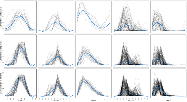
Figure 5: French Pollen Data results. Curves belonging to each single block with superimposed the corresponding block specific mean curve (in light blue).

Table 4: French map with overimposed the points indicating the cities colored according to their row cluster memberships (left) and Pollens organized by the column cluster memberships (right).

Row groups (Cities)	Column groups (Pollens)
	1	Gramineae, Urticaceae
	2	Chestnut, Plantain
	3	Cypress
	4	Ragweed, Mugwort, Birch, Beech,
		Morus, Olive, Platanus, Oak, Sorrel
		Linden
	5	Alder, Hornbeam, Hazel, Ash,
		Poplar, Willow

4.2.2 COVID-19 evolution across countries

At the time of writing this paper, an outbreak of infection with severe acute respiratory syndrome coronavirus 2 (SARS-CoV-2) has severely harmed the whole world. Countries all over the world have undertaken measures to reduce the spread of the virus: quarantine and social distancing practices have been implemented, collective events have been canceled or postponed, business and educational activities have been either interrupted or moved online.

While the outbreak has led to a global social and economic disruption, its spreading and evolution, also in relation to the aforementioned non pharmaceutical interventions, have not been the same all over the world (see Flaxman et al., 2020; Brauner et al., 2021, for an account of this in the first months of the pandemic). With this regard, the goal of the analysis is to evaluate differences and similarities among the countries and for different aspects of the pandemic.

Being the overall situation still evolving, and given that testing strategies have significantly changed across waves, we refer to the first wave of infection, considering the data from the 1st of March to the 4th of July 2020, in order to guarantee the consistency of the disease metrics used in the co-clustering. Moreover we restrict the analysis to the European countries. Data have been collected by the Oxford COVID-19 Government Response Tracker (OxCGRT, Hale et al., 2020) and originally refer to daily observations of the number of confirmed cases and deaths for COVID-19 in each country. We also select two indicators tracking the individual country intervention in response to the pandemic: the Stringency index and the Government response index. Both indicators are recorded on a 0-100 ordinal scale that represents the level of strictness of the policy and accounts for containment and closure policies. The latter indicator also reflects Health system policies such as information campaigns, testing strategies and contact tracing.

Data have been pre-processed as follows: daily values have been converted into weekly averages in order to reduce the impact of short term fluctuations and the number of time observations. Rates per 1000 inhabitants have been evaluated from the number of confirmed cases and deaths, and the logarithms applied to reduce the data skewness. All the variables have been standardized.

The resulting dataset is a matrix with $n=38$ rows (countries), $p$= 4 columns (variables describing the pandemic evolution and containment), observed over a period of $T=18$ weeks. Unlike the French Pollen data, here there is no strong reason to favour one random effect configuration over the others. Conversely, different configurations of random effects would entail different ideas of similarity of virus evolution. Thus, while the presence of random effects would allow to cluster together similar trends yet associated to different intensities, speed of evolution and time of onset, switching the random effects off could result in enhancing such differences via the separation of the trends.

Models have been run for $K=1,\ldots,6$ row clusters and $L=1,2,3$ column clusters, and all the 8 possible configurations of random effects. The behaviour of the resulting ICL values supports the remark in Section 4.1, as the criterion favours highly parameterized models. This holds particularly true with regard to the random effects configuration where the larger the number of random effects switched on, the highest the corresponding ICL. Thus, models with all the random effects switched on stand out among the others, with a preference for $K=2$ and $L=3$ whose results are displayed in Figure 6. The obtained partition is easily interpretable: in the column partition, reported on the right panel of Table 5, the containment indexes are grouped together into the same cluster whereas the log-rate of positiveness and death are singleton clusters. Consistently with the random effect configuration, row clusters exhibit a different evolution in terms of cases, deaths and undertaken containment measures: one cluster gathers countries where the virus has spread earlier and caused more losses; here, more severe control measures have been adopted, whose effect is likely seen in a general decreasing of cases and deaths after achieving a peak. The second row cluster collects countries for which the death toll of the pandemic seems to be more contained. The virus outbreak generally shows a delayed onset and a slower growth, which does not show a steep decline after reaching the peak, although the containment policies remain high for a long period. Notably, the row partition is also geographical, with the countries with higher mortality all belonging to the West Europe (see the left panel in Table 5).

To properly show the benefits of considering different random effects configurations in terms of notion and interpretation of the clusters, we also illustrate the partition produced by another model estimated having the three random effects switched off (Figure 7). Here we consider $K=L=3$: the column partition remains unchanged with respect to the best model, with the row partition still separating countries by the severity of the impact, with the third additional cluster having intermediate characteristics. According to this model, two row clusters feature countries with a similar right-skewed bell-shaped trend of cases and similar policies of containment, yet with a notable difference in the virus lethality. Indeed, the effect of switching $\alpha_{2}$ off is clearly noted in the log-rate of death fitting, with two mean curves having similar shapes but different scales. The additional intermediate cluster, less impacted in terms of death rate, is populated by countries from the central-east Europe. The apparent smaller impact of the first wave of the pandemic on the eastern European countries could be explained by several factors ranging from demographic characteristic and more timely closure policies to a different international mobility pattern. Additionally, other factors such as the general economic and health conditions might have prevented accurate testing and tracking policies, so that the actual spreading of the pandemic might have been underestimated.

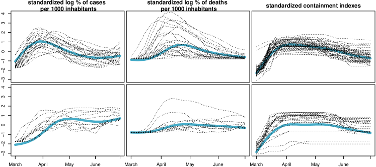
Figure 6: COVID-19 outgrowth results of the best model, with $K=2,$ $L=3$ and the three random effects on. Curves belonging to each single block with superimposed the associated block specific mean curve (in light blue).

Table 5: Europe map with countries colored according to their row cluster memberships (left) and variables organized by the column cluster membership (right) for the best ICL model.

Row groups (Countries)	Column groups (COVID-19 spreading and containment)
	1	log % of cases per 1000 inhabitants
	2	log % of deaths per 1000 inhabitants
	3	Stringency index, Government response index

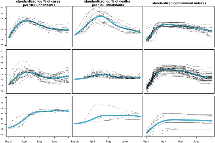
Figure 7: COVID-19 outgrowth results of the model with $K=3,$ $L=3$ and the three random effects off.

5 Conclusions

Modeling multivariate time-dependent data requires accounting for heterogeneity among subjects, capturing similarities and differences among variables, as well as correlations between repeated measures. Our work has tackled these challenges by proposing a new parametric co-clustering methodology, recasting the widely known Latent Block Model in a time-dependent fashion. The co-clustering model, by simultaneously searching for row and column clusters, partitions three-way matrices in blocks of homogeneous curves. Such approach takes into account the mentioned features of the data while building parsimonious and meaningful summaries. As a data generative mechanism for a single curve, we have considered the Shap Invariant Model that has turned out to be particularly flexible when embedded in a co-clustering context. The model allows to describe arbitrary time evolution patterns while adequately capturing dependencies among different temporal instants. The proposed method compares favorably with the few existing competitors for the simultaneous clustering of subjects and variables with time-dependent data. Our proposal, while producing co-partitions with comparable quality as measured by objective criteria, applies to both functional and longitudinal data, and has relevant advantages in terms of interpretability. The option of “switching off” some of the random effects, although in principle simplifying the model structure, increases its flexibility, as it allows to encompass different concepts of cluster possibly depending on the specific applications and on subject-matter considerations.

While further analyses are required to increase our understanding about the general performance of the proposed model, its application to both simulated and real data has provided overall satisfactory results and highlighted some aspects which worth further investigation. One interesting direction for future research is studying possible alternatives to the ICL to be used as selection tools when the model specification in the LBM framework involves random effects. Moreover, alternative choices, for example, for specifying the block mean curves, could be considered and compared with the choices adopted here. A further direction for future work would be exploring a fully Bayesian approach to model specification and estimation, possibly handling more easily the random parameters in the model.

References

- Anderlucci and Viroli [2015] L. Anderlucci and C. Viroli. Covariance pattern mixture models for the analysis of multivariate heterogeneous longitudinal data. The Annals of Applied Statistics, 9(2):777–800, 2015.
- Ben Slimen et al. [2018] Y.S. Ben Slimen, S. Allio, and J. Jacques. Model-based co-clustering for functional data. Neurocomputing, 291:97–108, 2018.
- Biernacki et al. [2000] C. Biernacki, G. Celeux, and G. Govaert. Assessing a mixture model for clustering with the integrated completed likelihood. IEEE transactions on pattern analysis and machine intelligence, 22(7):719–725, 2000.
- Bouveyron and Jacques [2011] C. Bouveyron and J. Jacques. Model-based clustering of time series in group-specific functional subspaces. Advances in Data Analysis and Classification, 5(4):281–300, 2011.
- Bouveyron et al. [2015] C. Bouveyron, E. Côme, and J. Jacques. The discriminative functional mixture model for a comparative analysis of bike sharing systems. The Annals of Applied Statistics, 9(4):1726–1760, 2015.
- Bouveyron et al. [2018] C. Bouveyron, L. Bozzi, J. Jacques, and F.X. Jollois. The functional latent block model for the co-clustering of electricity consumption curves. Journal of the Royal Statistical Society: Series C (Applied Statistics), 67(4):897–915, 2018.
- Bouveyron et al. [2019] C. Bouveyron, G. Celeux, T.B. Murphy, and A.E. Raftery. Model-Based Clustering and Classification for Data Science: With Applications in R. Cambridge University Press, 2019.
- Bouveyron et al. [2020] C. Bouveyron, J. Jacques, A. Schmutz, F. Simoes, and S. Bottini. Co-clustering of multivariate functional data for the analysis of air pollution in the south of france. HAL preprint hal-02862177, 2020.
- Brauner et al. [2021] J.M. Brauner, S. Mindermann, M. Sharma, D. Johnston, J. Salvatier, T. Gavenčiak, A.B. Stephenson, G. Leech, G. Altman, V. Mikulik, et al. Inferring the effectiveness of government interventions against COVID-19. Science, 371(6531), 2021.
- Corneli and Erosheva [2020] M. Corneli and E. Erosheva. A Bayesian approach for clustering and exact finite-sample model selection in longitudinal data mixtures. HAL preprint hal-02310069v2, 2020.
- Corneli et al. [2020] M. Corneli, C. Bouveyron, and P. Latouche. Co-clustering of ordinal data via latent continuous random variables and not missing at random entries. Journal of Computational and Graphical Statistics, 29(4):771–785, 2020.
- De Boor [1978] C. De Boor. A practical guide to splines. Springer-Verlag, New York, 1978.
- De la Cruz-Mesía et al. [2008] R. De la Cruz-Mesía, F. A Quintana, and G. Marshall. Model-based clustering for longitudinal data. Computational Statistics & Data Analysis, 52(3):1441–1457, 2008.
- Delattre et al. [2014] M. Delattre, M. Lavielle, and M. Poursat. A note on BIC in mixed-effects models. Electronic journal of statistics, 8(1):456–475, 2014.
- Dempster et al. [1977] A.P. Dempster, Nan M. Laird, and D.B. Rubin. Maximum likelihood from incomplete data via the em algorithm. Journal of the Royal Statistical Society: Series B (Methodological), 39(1):1–22, 1977.
- Diggle et al. [2002] P.J. Diggle, P. Heagerty, K.Y. Liang, P.J. Heagerty, and S. Zeger. Analysis of longitudinal data. Oxford University Press, 2002.
- Erosheva et al. [2014] E. Erosheva, R.L. Matsueda, and D. Telesca. Breaking bad: Two decades of life-course data analysis in criminology, developmental psychology, and beyond. Annual Review of Statistics and Its Application, 1:301–332, 2014.
- Flaxman et al. [2020] S. Flaxman, S. Mishra, A. Gandy, H.J.T. Unwin, T.A. Mellan, H. Coupland, C. Whittaker, H. Zhu, T. Berah, J.W. Eaton, et al. Estimating the effects of non-pharmaceutical interventions on COVID-19 in europe. Nature, 584(7820):257–261, 2020.
- Fraley and Raftery [2002] C. Fraley and A.E. Raftery. Model-based clustering, discriminant analysis, and density estimation. Journal of the American statistical Association, 97(458):611–631, 2002.
- Frühwirth-Schnatter [2011] S. Frühwirth-Schnatter. Panel data analysis: a survey on model-based clustering of time series. Advances in Data Analysis and Classification, 5(4):251–280, 2011.
- Govaert and Nadif [2003] G. Govaert and M. Nadif. Clustering with block mixture models. Pattern Recognition, 36(2):463–473, 2003.
- Govaert and Nadif [2008] G. Govaert and M. Nadif. Block clustering with bernoulli mixture models: Comparison of different approaches. Computational Statistics & Data Analysis, 52(6):3233–3245, 2008.
- Govaert and Nadif [2010] G. Govaert and M. Nadif. Latent block model for contingency table. Communications in Statistics - Theory and Methods, 39(3):416–425, 2010.
- Govaert and Nadif [2013] G. Govaert and M. Nadif. Co-clustering: models, algorithms and applications. John Wiley & Sons, 2013.
- Hale et al. [2020] T. Hale, N. Angrist, E. Cameron-Blake, L. Hallas, B. Kira, S. Majumdar, T. Petherick, A. Phillips, H. Tatlow, and S. Webster. Oxford COVID-19 Government Response Tracker, Blavatnik School of Government, 2020. URL https://www.bsg.ox.ac.uk/research/research-projects/coronavirus-government-response-tracker.
- Harring and Liu [2016] J.R. Harring and J. Liu. A comparison of estimation methods for nonlinear mixed-effects models under model misspecification and data sparseness: A simulation study. Journal of Modern Applied Statistical Methods, 15(1):27, 2016.
- Hubert and Arabie [1985] L. Hubert and P. Arabie. Comparing partitions. Journal of Classification, 2(1):193–218, 1985.
- Jacques and Biernacki [2018] J. Jacques and C. Biernacki. Model-based co-clustering for ordinal data. Computational Statistics & Data Analysis, 123:101–115, 2018.
- Jacques and Preda [2014] J. Jacques and C. Preda. Functional data clustering: a survey. Advances in Data Analysis and Classification, 8(3):231–255, 2014.
- Keribin et al. [2015] C. Keribin, V. Brault, G. Celeux, and G. Govaert. Estimation and selection for the latent block model on categorical data. Statistics and Computing, 25(6):1201–1216, 2015.
- Lawton et al. [1972] W.H. Lawton, E.A. Sylvestre, and M.S. Maggio. Self modeling nonlinear regression. Technometrics, 14(3):513–532, 1972.
- Liao [2005] T.W. Liao. Clustering of time series data - a survey. Pattern recognition, 38(11):1857–1874, 2005.
- Lindstrom [1995] M.J. Lindstrom. Self-modelling with random shift and scale parameters and a free-knot spline shape function. Statistics in Medicine, 14(18):2009–2021, 1995.
- Lindstrom and Bates [1990] M.J. Lindstrom and D. Bates. Nonlinear mixed effects models for repeated measures data. Biometrics, 46(3):673–687, 1990.
- Lomet [2012] A. Lomet. Sélection de modèle pour la classification croisée de données continues. PhD thesis, Compiègne, 2012.
- McNicholas and Murphy [2010] P.D. McNicholas and T.B. Murphy. Model-based clustering of longitudinal data. Canadian Journal of Statistics, 38(1):153–168, 2010.
- Nagin [2009] D. Nagin. Group-based modeling of development. Harvard University Press, 2009.
- Pinheiro and Bates [2006] J. Pinheiro and D. Bates. Mixed-effects models in S and S-PLUS. Springer Science & Business Media, 2006.
- Pinheiro et al. [2019] J. Pinheiro, D. Bates, S. DebRoy, D. Sarkar, and R Core Team. nlme: Linear and Nonlinear Mixed Effects Models, 2019. URL https://CRAN.R-project.org/package=nlme. R package version 3.1-139.
- R Core Team [2019] R Core Team. R: A Language and Environment for Statistical Computing. R Foundation for Statistical Computing, Vienna, Austria, 2019. URL https://www.R-project.org/.
- Ramsay and Li [1998] J.O. Ramsay and X. Li. Curve registration. Journal of the Royal Statistical Society: Series B (Methodological), 60(2):351–363, 1998.
- Ramsay and Silverman [2005] J.O. Ramsay and B.W. Silverman. Functional data analysis. Springer, New York, 2005.
- Rice [2004] J.A. Rice. Functional and longitudinal data analysis: perspectives on smoothing. Statistica Sinica, pages 631–647, 2004.
- Robert et al. [2020] V. Robert, Y. Vasseur, and V. Brault. Comparing high-dimensional partitions with the co-clustering adjusted rand index. Journal of Classification, pages 1–29, 2020.
- Selosse et al. [2020] M. Selosse, J. Jacques, and C. Biernacki. Model-based co-clustering for mixed type data. Computational Statistics & Data Analysis, 144:106866, 2020.
- Telesca and Inoue [2008] D. Telesca and L.Y.T. Inoue. Bayesian hierarchical curve registration. Journal of the American Statistical Association, 103(481):328–339, 2008.
- Telesca et al. [2012] D. Telesca, E. Erosheva, D. A Kreager, and R.L. Matsueda. Modeling criminal careers as departures from a unimodal population age–crime curve: the case of marijuana use. Journal of the American Statistical Association, 107(500):1427–1440, 2012.
- Viroli [2011a] C. Viroli. Finite mixtures of matrix normal distributions for classifying three-way data. Statistics and Computing, 21(4):511–522, 2011a.
- Viroli [2011b] C. Viroli. Model based clustering for three-way data structures. Bayesian Analysis, 6(4):573–602, 2011b.
- Wu [1983] C.J. Wu. On the convergence properties of the em algorithm. The Annals of statistics, pages 95–103, 1983.
- Wyse and Friel [2012] J. Wyse and N. Friel. Block clustering with collapsed latent block models. Statistics and Computing, 22(2):415–428, 2012.
- Wyse et al. [2017] J. Wyse, N. Friel, and P. Latouche. Inferring structure in bipartite networks using the latent blockmodel and exact ICL. Network Science, 5(1):45–69, 2017.