Concentration Inequalities for Two-Sample Rank Processes with Application to Bipartite Ranking

Abstract

The $\rm ROC$ curve is the gold standard for measuring the performance of a test/scoring statistic regarding its capacity to discriminate between two statistical populations in a wide variety of applications, ranging from anomaly detection in signal processing to information retrieval, through medical diagnosis. Most practical performance measures used in scoring/ranking applications such as the $\rm AUC$, the local $\rm AUC$, the $p$-norm push, the $\mathop{\rm DCG}$ and others, can be viewed as summaries of the $\rm ROC$ curve. In this paper, the fact that most of these empirical criteria can be expressed as two-sample linear rank statistics is highlighted and concentration inequalities for collections of such random variables, referred to as two-sample rank processes here, are proved, when indexed by VC classes of scoring functions. Based on these nonasymptotic bounds, the generalization capacity of empirical maximizers of a wide class of ranking performance criteria is next investigated from a theoretical perspective. It is also supported by empirical evidence through convincing numerical experiments.

1 Introduction

In the context of ranking, a variety of performance measures can be considered. In the simplest framework of bipartite ranking, where two independent i.i.d. samples $\mathbf{X}_{1},\;\ldots,\;\mathbf{X}_{n}$ and $\mathbf{Y}_{1},\;\ldots,\;\mathbf{Y}_{m}$ defined on the same probability space $(\Omega,\;\mathcal{F},\;\mathbb{P})$, valued in the same space ${\cal Z}$, say $\mathbb{R}^{d}$ with $d\geq 1$ for instance, and drawn from probability distributions $G$ and $H$ respectively (referred to as the ’positive distribution’ and the ’negative distribution’ respectively), the goal pursued is to learn a preorder on ${\cal Z}$ defined through a scoring function $s:{\cal Z}\rightarrow\mathbb{R}$ (which transports the natural order on the real line onto the feature space ${\cal Z}$) such that, for any random observation $\mathbf{Z}\in{\cal Z}$ sampled from a distribution that is equal either to the ’positive distribution’ or to the ’negative one’, the larger the score $s(z)$, the likelier it is drawn from the ’positive distribution’ $G$. Though easy to formulate, this simple framework encompasses many practical problems from the design of search engines in Information Retrieval (in this case, for a specific request, $G$ is the distribution of the relevant digitized documents, while $H$ is that of the irrelevant ones) to the elaboration of decision support tools in personalized medicine for instance. In spite of its simplicity there is not one and only one natural scalar criterion for evaluating the performance of a scoring rule $s(z)$, but many possible options. The Receiving Operator Characteric curve (the $\rm ROC$ curve in abbreviated form), i.e. the PP-plot of the false positive rate vs the true positive rate:

$$t\in\mathbb{R}\mapsto\left(\mathbb{P}\{s(\mathbf{Y})>t\},\;\mathbb{P}\{s(\mathbf{X})>t\}\right),$$

denoting by $\mathbf{X}$ and $\mathbf{Y}$ two generic r.v. with distributions $G$ and $H$ respectively, provides an exhaustive description of the performance of any scoring rule candidate $s$. However, its functional nature renders direct optimization strategies rather complex, see e.g. [10]. Empirical risk minimization methods (ERM) are thus generally based on summaries of the $\rm ROC$ curve, which take the form of empirical risk functionals where the averages involved are no longer taken over i.i.d. sequences. The most popular choice is undoubtedly the $\rm AUC$ criterion ($\rm AUC$ standing for Area Under the $\rm ROC$ Curve), see [1] or [4] for instance, but when focus is on top-ranked instances, various choices can be considered, e.g. the Discounted Cumulative Gain or DCG (see [11]), the $p$-norm push (see [30]), the local $\rm AUC$ (refer to [7]) or other variants such as those recently introduced in [26]. The present paper starts from the simple observation that most of these summary criteria have a common feature: they belong to the class of two-sample linear rank statistics. Such statistics have been extensively studied in the mathematical statistics literature because of their optimality properties in hypothesis testing, see [19]. They are widely used in order to test whether two samples are drawn from the same distribution against the alternative stipulating that the distribution of one of the samples is stochastically larger than the other. For instance, the empirical counterpart of the $\rm AUC$ of a scoring function $s(z)$ corresponds to the popular Mann-Withney-Wilcoxon statistic based on the two (univariate) samples $s(\mathbf{X}_{1}),\;\ldots,\;s(\mathbf{X}_{n})$ and $s(\mathbf{Y}_{1}),\;\ldots,\;s(\mathbf{Y}_{m})$. Other rank statistics can be considered, corresponding to other ways of measuring how the distribution of the ’positive score’ $s(\mathbf{X})$ is (possibly) stochastically larger than that of the ’negative score’ $s(\mathbf{Y})$. Now, in the statistical learning view, with the importance of excess risk bounds, the Empirical Risk Minimization paradigm must be revisited and new problems, mainly related to the uniform control of the fluctuations of collections of two-sample linear rank statistics, termed rank processes throughout the article, and to the measure of the complexity of nonparametric classes of scoring functions, come up. The arguments required to deal with risk functionals based on two-sample linear rank statistics have been sketched in [7] in a very special case.

In the present paper, we relate two-sample linear rank statistics to performance measures relevant for the ranking problem by showing that the target of ranking algorithms corresponds to optimal ordering rules in this sense and show that the generic structure of two-sample linear rank statistics as an orthogonal decomposition after projection onto the space of sums of i.i.d. random variables is the key to all statistical results related to maximizers of such criteria: consistency, rates of convergence or model selection. Notice incidentally that the empirical $\rm AUC$ is also a $U$-statistic and a decomposition method akin to that considered in this paper (though much less general) has been used in order to handle this specific dependence structure in [4]. In this article, concentration properties of two-sample rank processes (i.e. collections of two-sample linear rank statistics) are investigated using the linearization technique aforementioned. While interesting in themselves, the concentration inequalities established for this class of stochastic processes, when indexed by Vapnik-Chervonenkis classes (abbreviated with VC-classes) of scoring functions, are next applied to study the generalization capacity of empirical maximizers of a large collection of performance criteria based on two-sample linear rank statistics. Notice finally that a preliminary version of this work is briefly outlined in the conference paper [8]. This article presents a much deeper analysis of bipartite ranking via maximization of two-sample linear rank statistics. In particular, it offers a complete and detailed study of the concentration properties of two-sample rank processes (in a slightly different framework, stipulating that two independent i.i.d. samples, positive and negative, are observed, rather than classification data), provides model selection results and, from a practical perspective, tackles the issue of smoothing the risk functionals under study here with statistical learning guarantees.

The paper is organized as follows. In Section 2, the main notations are set out, the bipartite ranking problem is formulated as a statistical learning task in a rigorous probabilistic framework and the concept of two-sample linear rank statistic is briefly recalled. It is also explained that, unsurprisingly, natural performance criteria in bipartite ranking are of the form of two-sample (linear) rank statistics. Concentration results for rank processes, are established in Section 3. By means of the latter, performance of bipartite ranking rules obtained by maximizing two-sample linear rank statistics are investigated in Section 4. Finally, Section 5 displays illustrative experimental results, supporting the theoretical analysis carried out in the present article. Proofs, technical details and additional numerical results are deferred to the Appendix section.

2 Motivation and Preliminaries

We start with recalling key notions pertaining to $\rm ROC$ analysis and bipartite ranking, which essentially motivates the theoretical analysis carried out in the subsequent section. We next recall at length the definition of two-sample linear rank statistics, which have been intensively used to design statistical (homogeneity) testing procedures in the univariate setup, and finally highlight that many scalar summaries of empirical $\rm ROC$ curves, commonly used as ranking performance criteria, are precisely of this form. Here and throughout, the indicator function of any event $\mathcal{E}$ is denoted by $\mathbb{I}\{\mathcal{E}\}$, the Dirac mass at any point $x$ by $\delta_{x}$, the generalized inverse of any cumulative distribution function $W(t)$ on $\mathbb{R}\cup\{+\infty\}$ by $W^{-1}(u)=\inf\{t\in]-\infty,\;+\infty]:\;W(t)\geq u\}$, $u\in[0,1]$. We also denote the floor and ceiling functions by $u\in\mathbb{R}\mapsto\lfloor u\rfloor$ and by $u\in\mathbb{R}\mapsto\lceil u\rceil$ respectively.

2.1 Bipartite Ranking and $\rm ROC$ Analysis

As recalled in the Introduction section, the goal of bipartite ranking is to learn, based on independent ’positive’ and ’negative’ random samples $\{\mathbf{X}_{1},\;\ldots,\;\mathbf{X}_{n}\}$ and $\{\mathbf{Y}_{1},\;\ldots,\;\mathbf{Y}_{m}\}$, how to score any new observations $\mathbf{Z}_{1},\;\ldots,\;\mathbf{Z}_{k}$, being each either ’positive’ or else ’negative’, that is to say drawn either from $G$ or else from $H$, without prior knowledge, so that positive instances are mostly at the top of the resulting list with large probability. A natural way of defining a total preorder on ${\cal Z}$ is to map it with the natural order on $\mathbb{R}\cup\{+\infty\}$ by means of a scoring rule, i.e. a measurable mapping $s:{\cal Z}\rightarrow]-\infty,\;\infty]$. By $\mathcal{S}$ is denoted the set of all scoring rules. It is by means of $\rm ROC$ analysis that the capacity of a scoring rule candidate $s(z)$ to discriminate between the positive and negative statistical populations is generally evaluated.

$\rm ROC$ curves. The $\rm ROC$ curve is a gold standard to describe the dissimilarity between two univariate probability distributions $G$ and $H$. This criterion of functional nature, $\rm ROC_{H,G}$, can be defined as the parametrized curve in $[0,1]^{2}$:

$$t\in\mathbb{R}\mapsto\left(1-H(t),\;1-G(t)\right),$$

where possible jumps are connected by line segments, so as to ensure that the resulting curve is continuous. With this convention, one may then see the $\rm ROC$ curve related to the pair of d.f. $(H,G)$ as the graph of a càd-làg (i.e. right-continuous and left-limited) non decreasing mapping valued in $[0,1]$, defined by:

$$\alpha\in(0,1)\mapsto 1-G\circ H^{-1}(1-\alpha)~{},$$

at points $\alpha$ such that $G\circ H^{-1}(1-\alpha)=1-\alpha$. Denoting by ${\cal Z}_{H}$ and ${\cal Z}_{G}$ the supports of $H$ and $G$ respectively, observe that it connects the point $(0,1-G({\cal Z}_{H}))$ to $(H({\cal Z}_{G}),1)$ in the unit square $[0,1]^{2}$ and that, in absence of plateau (which we assume here for simplicity, rather than restricting the feature space to $G$’s support), the curve $\alpha\in(0,1)\mapsto\rm ROC_{G,H}(\alpha)$ is the image of $\alpha\in(0,1)\mapsto\rm ROC_{H,G}(\alpha)$ by the reflection with the main diagonal of the Euclidean plane (i.e. the line of equation ’$\beta=\alpha$’) as axis. Notice that the curve $\rm ROC_{H,G}$ coincides with the main diagonal of $[0,1]^{2}$ if and only if the two distributions $H$ and $G$ are equal. Hence, the concept of $\rm ROC$ curve offers a visual tool to examine the differences between two distributions in a pivotal manner, see Fig. 1. For instance, the univariate distribution $G(dt)$ is stochastically larger than $H(dt)$ if and only if the curve $\rm ROC_{H,G}$ is everywhere above the main diagonal and $\rm ROC_{H,G}$ coincides with the left upper corner of the unit square iff the essential supremum of the distribution $H$ is smaller than the essential infimum of the distribution $G$.

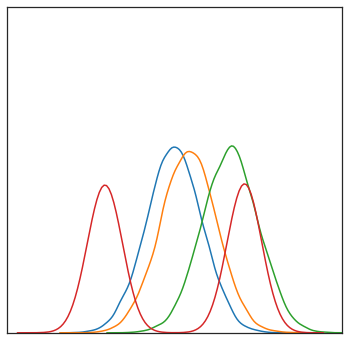
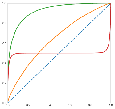
a. Probability distributions b. $\rm ROC$ curves

Figure 1: Examples of pairs of distributions and their related $\rm ROC$ curves. The ’negative’ distribution $H$ is represented in blue and three examples of ’positive’ distributions are represented in red, orange and green, like the associated $\rm ROC$ curves.

Another advantage of the $\rm ROC$ curve lies in the probabilistic interpretation of the popular $\rm ROC$ curve summary, referred to as the Area Under the $\rm ROC$ Curve ($\rm AUC$ in short)

$$\rm AUC_{H,G}\overset{def}{=}\int_{0}^{1}\rm ROC_{H,G}(\alpha)d\alpha=\mathbb{P}\left\{Y<X\right\}+\frac{1}{2}\mathbb{P}\left\{X=Y\right\},$$ (2.1)

where $(X,Y)$ denotes a pair of independent r.v.’s with respective marginal distributions $H$ and $G$.

Bipartite Ranking as $\rm ROC$ curve optimization. Going back to the multivariate setup, where $H$ and $G$ are probability distributions on ${\cal Z}$, say ${\cal Z}=\mathbb{R}^{d}$ with arbitrary dimension $d\geq 1$, the goal pursued in bipartite ranking can be phrased as that of building a scoring rule $s(z)$ such that the (univariate) distribution $G_{s}$ of $s(\mathbf{X})$ is ’as stochastically larger as possible’ than the the distribution $H_{s}$ of $s(\mathbf{Y})$. Hence, the capacity of a candidate $s(z)$ to discriminate between the positive and negative statistical populations can be evaluated by plotting the $\rm ROC$ curve $\alpha\in(0,1)\mapsto\rm ROC(s,\alpha)=\rm ROC_{H_{s},G_{s}}(\alpha)$: the closer to the left upper corner of the unit square the curve $\rm ROC(s,.)$, the better the scoring rule $s$. Therefore, the $\rm ROC$ curve conveys a partial preorder on the set of all scoring functions: for all pairs of scoring functions $s_{1}$ and $s_{2}$, one says that $s_{2}$ is more accurate than $s_{1}$ when $\rm ROC(s_{1},\alpha)\leq\rm ROC(s_{2},\alpha)$ for all $\alpha\in[0,1]$. It follows from a standard Neyman-Pearson argument that the most accurate scoring rules are increasing transforms of the likelihood ratio $\Psi(z)=dG/dH(z)$. Precisely, it is shown in [9] (see Proposition 2 therein) that the optimal scoring rules are the elements of the set:

$${\cal S}^{*}=\left\{s\in{\cal S}\;\text{ {s.t.} for all }z,\;z^{\prime}\text{ in }\mathbb{R}^{d}:\;\;\Psi(z)<\Psi(z^{\prime})\Rightarrow s^{*}(z)<s^{*}(z^{\prime})\right\}.$$ (2.2)

We denote by $\rm ROC^{*}(.)=\rm ROC(\Psi,\;.)$ and recall incidentally that this optimal curve is non-decreasing and concave and thus always above the main diagonal of the unit square. Now, the bipartite ranking task can be reformulated in a more quantitative manner: the objective pursued is to build a scoring function $s(z)$, based on the training examples $\{\mathbf{X}_{1},\;\ldots,\;\mathbf{X}_{n}\}\text{ and }\{\mathbf{Y}_{1},\;\ldots,\;\mathbf{Y}_{m}\}$, with a $\rm ROC$ curve as close as possible to $\rm ROC^{*}$. A typical way of measuring the deviation between the two curves is to consider the distance in $\sup$ norm:

$$d_{\infty}(s,s^{*})=\sup_{\alpha\in(0,1)}\left|\rm ROC(s,\alpha)-\rm ROC^{*}(\alpha)\right|~{}.$$ (2.3)

Attention should be paid that this quantity is a distance between $\rm ROC$ curves (or between the related equivalence classes of scoring functions, the $\rm ROC$ curve of any scoring function being invariant by strictly increasing transform) not between the scoring functions themselves. Since the curve $\rm ROC^{*}$ is unknown in practice, the major difficulty lies in the fact that no straightforward statistical counterpart of the (functional) loss (2.3) is available. In [9] (see also [10]), it has been however shown that bipartite ranking can be viewed as a superposition of cost-sensitive classification problems and somehow ’discretized’ in an adaptive manner, so as to apply empirical risk minimization with statistical guarantees in the $d_{\infty}$-sense, at the price of an additional bias term inherent to the approximation step. Alternatively, the performance of a candidate scoring rule $s$ can be measured by means of the $L_{1}$-norm in the $\rm ROC$ space. Observing that, in this case, the loss can be decomposed as follows:

$$d_{1}(s,s^{*})=\int_{0}^{1}|\rm ROC(s,\alpha)-\rm ROC^{*}(\alpha)|d\alpha=\int_{0}^{1}\rm ROC^{*}(\alpha)d\alpha-\int_{0}^{1}\rm ROC(s,\alpha)d\alpha~{},$$ (2.4)

minimizing the $L_{1}$-distance to the optimal $\rm ROC$ curve boils down to maximizing the area under the curve $\rm ROC(s,\;.)$, that is to say

$$\rm AUC(s)\overset{def}{=}\rm AUC_{H_{s},G_{s}}=\mathbb{P}\{s(\mathbf{Y})<s(\mathbf{X})\}+\frac{1}{2}\mathbb{P}\{s(\mathbf{Y})=s(\mathbf{X})\}~{},$$ (2.5)

where $\mathbf{X}$ and $\mathbf{Y}$ are random variables defined on the same probability space, independent, with respective distributions $G$ and $H$, denoting by $G_{s}$ and $H_{s}$ the distributions of $s(\mathbf{X})$ and $s(\mathbf{Y})$ respectively. The scalar performance criterion $\rm AUC(s)$ defines a total preorder on $\mathcal{S}$ and its maximal value is denoted by $\rm AUC^{*}=\rm AUC(s^{*})$, with $s^{*}\in{\cal S}^{*}$. Bipartite ranking through maximization of empirical versions of the $\rm AUC$ criterion has been studied in several articles, including [1] or [4]. Extension to multipartite ranking (i.e. when the number of samples/distributions under study is larger than $3$) is considered in [6], see also [5]. In contrast to [9] or [10], where the task of learning scoring rules with statistical guarantees in $\sup$ norm in the $\rm ROC$ space is considered, the present article focuses on optimization of summary scalar empirical criteria generalizing the $\rm AUC$ that takes the form of two-sample linear rank statistics, as could be naturally expected when addressing ranking problems.

2.2 Two-Sample Linear Rank Statistics

If the curve $\rm ROC_{H,G}$ is the appropriate tool to examine to which extent a univariate distribution $G$ is stochastically larger than another one $H$, practical decisions are generally made on the basis of the observations of two univariate independent random i.i.d. samples $\{X_{1},\;\ldots,\;X_{n}\}$ and $\{Y_{1},\;\ldots,\;Y_{m}\}$, drawn from $G$ and $H$ respectively. Computing the empirical cumulative distribution functions $\widehat{H}_{m}(t)=(1/m)\sum_{j=1}^{m}\mathbb{I}\{Y_{j}\leq t\}$ and $\widehat{G}_{n}(t)=(1/n)\sum_{i=1}^{n}\mathbb{I}\{X_{i}\leq t\}$ for $t\in\mathbb{R}$, one can plot the empirical $\rm ROC$ curve:

$$\widehat{\rm ROC}=\rm ROC_{\widehat{H}_{m},\;\widehat{G}_{n}}.$$ (2.6)

Observe that the $\rm ROC$ curve (2.6) is an increasing broken line connecting $(0,0)$ to $(1,1)$ in the unit square $[0,1]^{2}$ and is fully determined by the set of ranks occupied by the positive instances within the pooled sample $\{\mathop{\rm Rank}(X_{i}):\;i=1,\;\ldots,\;n\}$, where:

$$\forall i\in\{1,\;\ldots,\;n\}\quad\mathop{\rm Rank}(X_{i})=N\widehat{F}_{N}(X_{i})~{},$$ (2.7)

with $\widehat{F}_{N}(t)=(1/N)\sum_{i=1}^{n}\mathbb{I}\{X_{i}\leq t\}+(1/N)\sum_{j=1}^{m}\mathbb{I}\{Y_{j}\leq t\}$ and $N=n+m$. Breakpoints of the piecewise linear curve (2.6) necessarily belong to the set of gridpoints $\left\{\left(j/m,\;i/n\right):\;j\in\{1,\;\ldots,\;m-1\}\text{ and }i\in\{1,\;\ldots,\;n-1\}\right\}$. Denote by $X_{(i)}$ the order statistics related to the sample $\{X_{1},\;\ldots,\;X_{n}\}$, i.e. $\mathop{\rm Rank}(X_{(n)})>\cdots>\mathop{\rm Rank}(X_{(1)})$, and by $Y_{(j)}$ those related to the sample $\{Y_{1},\;\ldots,\;Y_{m}\}$. Consider the càd-làg step function:

$$\alpha\in[0,1]\mapsto\sum_{j=1}^{m}\widehat{\gamma}_{j}\cdot\mathbb{I}\{\alpha\in[(j-1)/m,\;j/m[\}~{},$$ (2.8)

where, for all $j\in\{1,\;\ldots,\;m\}$, we set:

$$\widehat{\gamma}_{j}=\frac{1}{n}\sum_{i=1}^{n}\mathbb{I}\{X_{i}>Y_{(m-j+1)}\}=\frac{1}{n}\sum_{i=1}^{n}\mathbb{I}\{\mathop{\rm Rank}(X_{(n-i+1)})>\mathop{\rm Rank}(Y_{(m-j+1)})\}\\ =\frac{1}{n}\sum_{i=1}^{n}\mathbb{I}\{j\geq N-\mathop{\rm Rank}(X_{(n-i+1)})-i+2\}~{}.$$

The $\rm ROC$ curve (2.6) is the continuous broken line that connects the jump points of the step curve (2.8) and can thus be expressed as a function of the ’positive ranks’ i.e. the $\mathop{\rm Rank}(X_{i})$’s only. As a consequence, any summary of the empirical $\rm ROC$ curve, is a two-sample rank statistic, that is a measurable function of the ’positive ranks’. In particular, the empirical $\rm AUC$, i.e. the $\rm AUC$ of the empirical $\rm ROC$ curve (2.6), also termed the rate of concording pairs or the Mann-Whitney statistic, can be easily shown to coincide, up to an affine transform, with the sum of ’positive ranks’, the well-known rank-sum Wilcoxon statistic [37]:

$$\widehat{W}_{n,m}=\sum_{i=1}^{n}\mathop{\rm Rank}(X_{i})~{}.$$ (2.9)

Indeed, we have:

$$\widehat{W}_{n,m}=nm\rm AUC_{\widehat{H}_{m},\widehat{G}_{n}}+\frac{n(n+1)}{2}~{}.$$

However, two-sample rank statistics (i.e. functions of the $\mathop{\rm Rank}(X_{i})$’s) form a very rich collection of statistics and this is by no means the sole possible choice to summarize the empirical $\rm ROC$ curve.

Definition. 1.

(Two-sample linear rank statistics) Let $\phi:[0,1]\rightarrow\mathbb{R}$ be a nondecreasing function. The two-sample linear rank statistics with ’score-generating function’ $\phi(u)$ based on the random samples $\{X_{1},\;\ldots,\;X_{n}\}$ and $\{Y_{1},\;\ldots,\;Y_{m}\}$ is given by:

$$\widehat{W}^{\phi}_{n,m}=\sum_{i=1}^{n}\phi\left(\frac{\mathop{\rm Rank}(X_{i})}{N+1}\right).$$ (2.10)

The statistics (2.10) defined above are all distribution-free when $H=G$ and are, for this reason, particularly useful to detect differences between the distributions $H$ and $G$ and widely used to perform homogeneity tests in the univariate setup. Tabulating their distribution under the null assumption, they can be used to design unbiased tests at certain levels $\alpha$ in $(0,1)$. The choice of the score-generating function $\phi$ can be guided by the type of difference between the two distributions (e.g. in scale, in location) one possibly expects, and may then lead to locally most powerful testing procedures, capable of detecting ’small’ deviations from the homogeneous situation. More generally, depending on the statistical test to perform, one may use particular function $\phi$, Figure 2 shows classic score-generating functions broadly used for two-sample statistical tests (refer to [17]). One may refer to Chapter 9 in [31] or to Chapter 13 in [35] for an account of the (asymptotic) theory of rank statistics. In the present paper, two-sample linear rank statistics are used for a very different purpose, as empirical performance measures in bipartite ranking based on two independent multivariate samples $\{\mathbf{X}_{1},\;\ldots,\;\mathbf{X}_{n}\}$ and $\{\mathbf{Y}_{1},\;\ldots,\;\mathbf{Y}_{m}\}$. The analysis of the bipartite ranking problem carried out in Section 4, based on the concentration inequalities established in Section 3, shows the relevance of evaluating the ranking performance of a scoring rule candidate $s(z)$ by computing a two-sample linear rank statistic based on the univariate samples obtained after scoring $\{s(\mathbf{X}_{1}),\;\ldots,\;s(\mathbf{X}_{n})\}$ and $\{s(\mathbf{Y}_{1}),\;\ldots,\;s(\mathbf{Y}_{m})\}$ and establishes statistical guarantees for the generalization capacity of scoring rules built by optimizing such an empirical criterion.

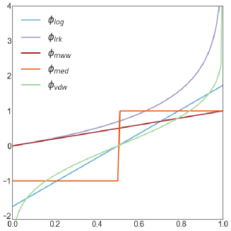
Figure 2: Curves of two-sample score-generating functions with the associated statistical test: Logistic test $\phi_{log}(u)=2\sqrt{3}(u-1/2)$ in blue, Logrank test $\phi_{lrk}(u)=-\log(1-x)$ in purple, Mann-Whitney-Wilcoxon test $\phi_{mww}(u)=u$ in red, Median test $\phi_{med}(u)=\mathop{\rm sgn}(u-1/2)$ in orange, Van der Waerden test $\phi_{vdw}(u)=\Phi^{-1}(u)$ in green, $\Phi$ being the normal quantile function.

2.3 Bipartite Ranking as Maximization of Two-Sample Rank Statistics

As foreshadowed above, empirical performance measures in bipartite ranking should be unsurprisingly based on ranks. We propose here to evaluate empirically the ranking performance of any scoring function candidate $s(z)$ in $\mathcal{S}$ by means of statistics of the type:

$$\widehat{W}^{\phi}_{n,m}(s)=\sum_{i=1}^{n}\phi\left(\frac{\mathop{\rm Rank}(s(\mathbf{X}_{i}))}{N+1}\right),$$ (2.11)

where $N=n+m$, $\phi:[0,1]\to\mathbb{R}$ is some Borelian nondecreasing function. This quantity is a two-sample linear rank statistic (see Definition 1) related to the score-generating function $\phi(u)$ and the samples $\{s(\mathbf{X}_{1}),\;\ldots,\;s(\mathbf{X}_{n})\}$ and $\{s(\mathbf{Y}_{1}),\;\ldots,\;s(\mathbf{Y}_{m})\}$. This statistic is invariant by increasing transform of the scoring function $s$, just like the (empirical) $\rm ROC$ curve and, as recalled in the previous section, it is a natural and common choice to quantify differences in distribution between the univariate samples $\{s(\mathbf{X}_{1}),\;\ldots,\;s(\mathbf{X}_{n})\}$ and $\{s(\mathbf{Y}_{1}),\;\ldots,\;s(\mathbf{Y}_{m})\}$, to evaluate to which extent the distribution of the first sample is stochastically larger than that of the second sample in particular. It consequently appears as legitimate to learn a scoring function $s$ by maximizing the criterion (2.11). Whereas rigorous arguments are developed in Section 4, we highlight here that, for specific choices of the score-generating function $\phi$, many relevant criteria considered in the ranking literature can be accurately approximated by statistics of this form:

• $\phi(u)=u$ - this choice leads to the celebrated Wilcoxon-Mann-Whitney statistic which is related to the empirical version of the $\rm AUC$.

• $\phi(u)=u\mathbb{I}\{u\geq u_{0}\}$, for some $u_{0}\in(0,1)$ - such a score-generating function corresponds to the local $\rm AUC$ criterion, introduced recently in [7]. Such a criterion is of interest when one wants to focus on the highest ranks.

• $\phi(u)=u^{q}$ - this is another choice which puts emphasis on high ranks but in a smoother way than the previous one. This is related to the $q$-norm push approach taken in [30]. However, we point out that the criterion studied in the latter work relies on a different definition of the rank of an observation. Namely, the rank of positive instances among negative instances (and not in the pooled sample) is used. This choice permits to use independence which makes the technical part much simpler, at the price of increasing the variance of the criterion.

• $\phi(u)=\phi_{N}(u)=c\left((N+1)u\right)\mathbb{I}\{u\geq k/(N+1)\}$ - this corresponds to the $\mathop{\rm DCG}$ criterion in the bipartite setup (see [11]), one of the ’gold standard quality measure’ in information retrieval, when grades are binary. The $c(i)$’s denote the discount factors, $c(i)$ measuring the importance of rank $i$. The integer $k$ denotes the number of top-ranked instances to take into account. Notice that, with our indexation, top positions correspond to the largest ranks and the sequence $\{c(i)\}_{i\leq N}$ should be chosen increasing.

Depending on the choice of the score-generating function $\phi$, some specific patterns of the preorder induced by a scoring function $s(z)$ can be either enhanced by the criterion (2.11) or else completely disappear: for instance, the value of (2.11) is essentially determined by the possible presence of positive instances among top-ranked observations, when considering a score generating function $\phi$ that rapidly vanishes near $0$ and takes much higher values near $1$.

Investigating the performance of maximizers of the criterion (2.11) from a nonasymptotic perspective is however far from straightforward, due to the complexity of the latter (i.e. a sum of strongly dependent random variables). It requires in particular to prove concentration inequalities for collections of two-sample linear rank statistics, indexed by classes of scoring functions of controlled complexity (i.e. of VC-type), referred to as two-sample rank processes throughout the article. It is the purpose of the next section to establish such results.

3 Concentration Inequalities for Two-Sample Rank Processes

This section is devoted to prove concentration bounds for collections of two-sample linear rank statistics (2.11), indexed by classes $\mathcal{S}_{0}\subset\mathcal{S}$ of scoring functions. In order to study the fluctuations of (2.11) as the full sample size $N$ increases, it is of course required to control the fraction of ’positive’/’negative’ observations in the pooled dataset. Let $p\in(0,1)$ be the ’theoretical’ fraction of positive instances. For $N\geq 1/p$, we suppose that $n=\lfloor pN\rfloor$ and $m=\lceil(1-p)N\rceil=N-n$. Define the mixture probability distribution $F=pG+(1-p)H$. For any $s\in\mathcal{S}$, the distribution of $s(\mathbf{X})$ (i.e. the image of $G$ by $s$) is denoted by $G_{s}$, that of $s(\mathbf{Y})$ (i.e. the image of $H$ by $s$) by $H_{s}$. We also denote by $F_{s}$ the image of distribution $F$ by $s$. For simplicity, the same notations are used to mean the related cumulative distribution functions. We also introduce their statistical versions $\widehat{G}_{s,n}(t)=(1/n)\sum_{i=1}^{n}\mathbb{I}\{s(\mathbf{X}_{i})\leq t\}$ and $\widehat{H}_{s,m}(t)=(1/m)\sum_{j=1}^{m}\mathbb{I}\{s(\mathbf{Y}_{j})\leq t\}$ and define:

$$\widehat{F}_{s,N}(t)=(n/N)\widehat{G}_{s,n}(t)+(m/N)\widehat{H}_{s,m}(t)~{}.$$ (3.1)

Since $n/N\rightarrow p$ as $N$ tends to infinity, the quantity above is a natural estimator of the c.d.f. $F_{s}$. Equipped with these notations, we can write:

$$\frac{1}{n}\widehat{W}^{\phi}_{n,m}(s)=\frac{1}{n}\sum_{i=1}^{n}\phi\left(\frac{N}{N+1}\widehat{F}_{s,N}(s(\mathbf{X}_{i}))\right).$$ (3.2)

Hence, the statistic (3.2) can be naturally seen as an empirical version of the quantity defined below, around which it fluctuates.

Definition. 2.

For a given score-generating function $\phi$, the functional

$$W_{\phi}(s)=\mathbb{E}[(\phi\circ F_{s})(s(\mathbf{X}))]~{},$$ (3.3)

is referred to as the ”$W_{\phi}$-ranking performance measure”.

Indeed, replacing $\widehat{F}_{s,N}(s(\mathbf{X}_{i}))$ in (3.2) by $F_{s}(s(\mathbf{X}_{i}))$ and taking next the expectation permits to recover $\eqref{eq:Wtrue}$. Observe in addition that, for $\phi(u)=u$, the quantity (3.3) is equal to $\rm AUC(s)$ (2.5) a soon as the distribution $F_{s}$ is continuous. The next lemma reveals that the criterion (3.3) can be viewed as a scalar summary of the $\rm ROC$ curve.

Lemma. 3.

Let $\phi$ be a score-generating function. We have, for all $s$ in ${\cal S}$,

$$W_{\phi}(s)=\frac{1}{p}\int_{0}^{1}\phi(u)du-\frac{1-p}{p}\int_{0}^{1}\phi\left(p(1-\rm ROC(s,\alpha))+(1-p)(1-\alpha)\right)~{}d\alpha~{}.$$ (3.4)

proof. Using the decomposition $F_{s}=pG_{s}+(1-p)H_{s}$, we are led to the following expression:

$$pW_{\phi}(s)=\int_{0}^{1}\phi(u)~{}du-(1-p)\mathbb{E}[(\phi\circ F_{s})(s(\mathbf{Y}))]~{}.$$

Then, using a change of variable, we get:

$$\mathbb{E}[(\phi\circ F_{s})(s(\mathbf{Y}))]=\int_{0}^{1}\phi(p(1-\rm ROC(s,\alpha))+(1-p)(1-\alpha))~{}d\alpha~{}.$$

As revealed by Eq. (3.4), a score-generating function $\phi$ that takes much higher values near $1$ than near $0$ defines a criterion (3.3) that mainly summarizes the behavior of the $\rm ROC$ curve near the origin, i.e. the preorder on the set of instances with highest scores.

Below, we investigate the concentration properties of the process:

$$\left\{\frac{1}{n}\widehat{W}^{\phi}_{n,m}(s)-W_{\phi}(s)\right\}_{s\in\mathcal{S}_{0}}.$$ (3.5)

As a first go, we prove, by means of linearization techniques, that two-sample linear rank statistics can be uniformly approximated by much simpler quantities, involving i.i.d. averages and two-sample $U$-statistics. This will be key to establish probability bounds for the maximal deviation:

$$\sup_{s\in\mathcal{S}_{0}}\left|\frac{1}{n}\widehat{W}^{\phi}_{n,m}(s)-W_{\phi}(s)\right|,$$ (3.6)

under adequate complexity assumptions for the class $\mathcal{S}_{0}$ of scoring functions considered and to study next the generalization ability of maximizers of the empirical criterion (3.2) in terms of $W_{\phi}$-ranking performance. Throughout the article, all the suprema considered, such as (3.6), are assumed to be measurable and we refer to Chapter 2.3 in [36] for more details on the formulation in terms of outer measure/expectation that guarantees measurability.

Uniform approximation of two-sample linear rank statistics. Whereas statistical guarantees for Empirical Risk Minimization in the context of classification or regression can be directly obtained by means of classic concentration results for empirical processes (i.e. averages of i.i.d. random variables), the study of the fluctuations of the process (3.5) is far from straightforward, insofar as the terms averaged in (3.2) are not independent. For averages of non-i.i.d. random variables, the underlying statistical structure can be revealed by orthogonal projections onto the space of sums of i.i.d. random variables in many situations. This projection argument was the key for the study of empirical $\rm AUC$ maximization or that of within cluster point scatter, which involved $U$-processes, see [4] and [3]. In the case of $U$-statistics, this orthogonal decomposition is known as the Hoeffding decomposition and the remainder may be expressed as a degenerate $U$-statistic, see [20]. For rank statistics, a similar though more complex decomposition can be considered. We refer to [18] for a systematic use of the projection method for investigating the asymptotic properties of general statistics. From the perspective of ERM in statistical learning theory, through the projection method, well-known concentration results for standard empirical processes and $U$-processes may carry over to more complex collections of random variables such as two-sample linear rank processes, as revealed by the approximation result stated below. It holds true under the following technical assumptions.

Assumption 1.

Let $M>0$. For all $s\in{\cal S}_{0}$, the random variables $s(\mathbf{X})$ and $s(\mathbf{Y})$ are continuous, with density functions that are twice differentiable and have Sobolev $\mathcal{W}^{2,\infty}$-norms bounded by $M<+\infty$.

Assumption 2.

The score-generating function $\phi:[0,1]\mapsto\mathbb{R}$, is nondecreasing and twice continuously differentiable.

Assumption 3.

The class of scoring functions ${\cal S}_{0}$ is a VC class of finite VC dimension ${\cal V}<+\infty$.

For the definition of VC classes of functions, one may refer to e.g. [36], see section 2.6.2 therein, and also recalled in Appendix section A.3. By means of the proposition below, the study of the fluctuations of the two-sample linear rank process (3.5) boils down to that of basic empirical processes.

Proposition. 4.

Suppose that Assumptions 1-3 are fulfilled. The two-sample linear rank process (3.5) can be linearized/decomposed as follows. For all $s\in{\cal S}_{0}$,

$$\widehat{W}_{n,m}^{\phi}(s)=n\widehat{W}_{\phi}(s)+\left(\widehat{V}_{n}^{X}(s)-\mathbb{E}\left[\widehat{V}_{n}^{X}(s)\right]\right)+\left(\widehat{V}_{m}^{Y}(s)-\mathbb{E}\left[\widehat{V}_{m}^{Y}(s)\right]\right)+\mathcal{R}_{n,m}(s)~{},$$ (3.7)

where

$$\widehat{W}_{\phi}(s) = \frac{1}{n}\sum_{i=1}^{n}\left(\phi\circ F_{s}\right)(s(\mathbf{X}_{i}))~{},$$

$$\widehat{V}_{n}^{X}(s) = \frac{n-1}{N+1}\sum_{i=1}^{n}\int_{s(\mathbf{X}_{i})}^{+\infty}(\phi^{\prime}\circ F_{s})(u)dG_{s}(u)~{},$$

$$\widehat{V}_{m}^{Y}(s) = \frac{n}{N+1}\sum_{j=1}^{m}\int_{s(\mathbf{Y}_{j})}^{+\infty}(\phi^{\prime}\circ F_{s})(u)dG_{s}(u)~{}.$$

For any $\delta\in(0,1)$, there exist constants $c_{1},\;c_{3}>0,\;c_{2}\geq 1,\;c_{4}>6,\;c_{5}>3$, depending on $\phi$ and ${\cal V}$, such that

$$\mathbb{P}\left\{\sup_{s\in{\cal S}_{0}}|\mathcal{R}_{n,m}(s)|<t\right\}\geq 1-\delta~{},$$ (3.8)

where $t=c_{1}+c_{2}\log(c_{4}/\delta)$ as soon as $N\geq(c_{3}/p)\log(c_{5}/\delta)$.

The proof of this linearization result is detailed in the Appendix section B.1 (refer to it for a description of the constants involved in the bound stated above). Its main argument consists in decomposing (3.2) by means of a Taylor expansion at order two of the score generating function $\phi(u)$ and applying next the Hájek orthogonal projection technique (recalled at length in the Introduction Lemma A.1 for completeness) to the component corresponding to the first order term. The quantity $\mathcal{R}_{n,m}(s)$ is then formed by bringing together the remainder of the Hájek projection and the component corresponding to the second order term of the Taylor expansion, while the probabilistic control of its order of magnitude is established by means of concentration results for (degenerate) one/two-sample $U$-processes (see the Appendix section A.4 for more details). It follows from decomposition (3.7) combined with triangular inequality that:

$$\sup_{s\in{\cal S}_{0}}\left|\frac{1}{n}\widehat{W}_{n,m}^{\phi}(s)-W_{\phi}(s)\right|\leq\sup_{s\in{\cal S}_{0}}\left|\widehat{W}_{\phi}(s)-W_{\phi}(s)\right|\\ +\sup_{s\in{\cal S}_{0}}\frac{1}{n}\left|\widehat{V}_{n}^{X}(s)-\mathbb{E}\left[\widehat{V}_{n}^{X}(s)\right]\right|+\sup_{s\in{\cal S}_{0}}\frac{1}{n}\left|\widehat{V}_{m}^{Y}(s)-\mathbb{E}\left[\widehat{V}_{m}^{Y}(s)\right]\right|\\ +\sup_{s\in{\cal S}_{0}}\frac{1}{n}\left|\mathcal{R}_{n,m}(s)\right|.$$ (3.9)

Hence, nonasymptotic bounds for the maximal deviation of the process (3.5) can be deduced from concentration inequalities for standard empirical processes, as shall be seen below. Before this, a few comments are in order.

Remark 1.

(On the complexity assumption) We point out that alternative complexity measures could be naturally considered, such as those based on Rademacher averages, see e.g. [22]. However, as different types of stochastic process (i.e. empirical process, degenerate one-sample $U$-process and degenerate two-sample $U$-process) are involved in the present nonasymptotic study, different types of Rademacher complexities (see e.g. [4]) should be introduced to control their fluctuations as well. For the sake of simplicity, the concept of VC-type class of functions is used here.

Remark 2.

(Smooth score-generating functions) The subsequent analysis is restricted to the case of smooth score-generating functions for simplification purposes. We nevertheless point out that, although one may always build smooth approximants of irregular score generating functions, the theoretical results established below can be directly extended to non-smooth situations, at the price of a significantly greater technical complexity.

The theorem below provides a concentration bound for the two-sample rank process (3.5). The proof is based on the uniform approximation result precedingly established, refer to the Appendix section B.3 for technical details.

Theorem. 5.

Suppose that the assumptions of Proposition 4 are fulfilled. Then, there exist constants $C_{1},\;C_{2}\geq 24$, depending on $\phi,\;{\cal V}$, such that for all $C_{4}\geq C_{1}$ depending on $\phi$, and $t$:

$$\mathbb{P}\left\{\sup_{s\in{\cal S}_{0}}\bigg{|}\frac{1}{n}\widehat{W}^{\phi}_{n,m}(s)-W_{\phi}(s)\bigg{|}>t\right\}\leq C_{2}e^{-pC_{3}Nt^{2}}~{},$$ (3.10)

as soon as $C_{1}/\sqrt{pN}\leq t\leq C_{4}\min(p,1-p)$, where $C_{3}=\log(1+C_{4}/(4C_{2}))/(C_{2}C_{4})$ depends on $\phi,\;{\cal V}$.

The concentration inequalities stated above are extensively used in the next section to study the ranking bipartite learning problem, when formulated as $W_{\phi}$-ranking performance maximization.

4 Performance of Maximizers of Two-Sample Rank Statistics in Bipartite Ranking

This section provides a theoretical analysis of bipartite ranking methods, based on maximization of the empirical ranking performance measure (2.11). While the concentration inequalities established in the previous section are the key technical tools to derive nonasymptotic bounds for the deficit of $W_{\phi}$-ranking performance measure of empirical maximizers, we start by showing that the criterion (3.3) is relevant to measure ranking performance, whatever the score generating function $\phi$ is chosen, beyond the examples listed in Subsection 2.3.

Optimal elements. The next result states that optimal scoring functions do maximize the $W_{\phi}$-ranking performance and form a collection that coincides with the set $\mathcal{S}^{*}_{\phi}$ of maximizers of (3.3), provided that the score-generating function $\phi$ is strictly increasing on $(0,1)$.

Proposition. 6.

Let $\phi$ be a score-generating function. The assertions below hold true.

• For all $(s,\;s^{*})\in{\cal S}\times{\cal S}^{*}$, we have $W_{\phi}(s)\leq W_{\phi}(s^{*})=W_{\phi}^{*}$, where $W_{\phi}^{*}\overset{def}{=}W_{\phi}(\Psi)$.

• Assuming in addition that the score-generating function $\phi$ is strictly increasing on $(0,1)$, we have: $\mathcal{S}^{*}_{\phi}={\cal S}^{*}$.

The proof immediately results from (3.4) combined with the fact that the $\rm ROC$ curve of increasing transforms of the likelihood ratio $\Psi(z)$ dominates everywhere any other $\rm ROC$ curve, as recalled in Section 2.1: $\forall(s,\;s^{*})\in{\cal S}\times{\cal S}^{*}$, $\forall\alpha\in(0,\;1)$, $\rm ROC(s,\alpha)\leq\rm ROC(s^{*},\alpha)=\rm ROC^{*}(\alpha)$. Details are left to the reader.

Remark 3.

(On plug-in ranking rules) Theoretically, a possible approach to bipartite ranking is the plug-in method ([12]), which consists of using an estimate $\hat{\Psi}$ of the likelihood function as a scoring function. As shown by the subsequent bound, when $\phi$ is differentiable with a bounded derivative, when $\hat{\Psi}$ is close to $\Psi$ in the $L_{1}$-sense, it leads to a nearly optimal ordering in terms of W-ranking criterion:

$$W_{\phi}^{*}-W_{\phi}\left(\widehat{\Psi}\right)\leq(1-p)||\phi^{\prime}||_{\infty}{\mathbb{E}}[|\widehat{\Psi}(\mathbf{X})-\Psi(\mathbf{X})|]~{}.$$

However, the bound above may be loose and the plug-in approach faces computational difficulties when dealing with high-dimensional data, see [16], which provide the motivation for exploring algorithms based on $W_{\phi}$-ranking performance maximization.

Remark 4.

(Alternative probabilistic framework) We point out that the present analysis can be extended to the alternative setup, where, rather than assuming that two samples of sizes $n$ and $m$, ’positive’ and ’negative’, are available for the learning tasks considered in this paper, the i.i.d. observations $Z$ are supposed to come with a random label $Y$ either equal to $+1$ or else to $-1$, indicating whether $Z$ is distributed according to $G$ or $H$. If $p$ denotes the probability that the label $Y$ is equal to $1$, the number $n$ of positive observations among a training sample of size $N$ is then random, distributed as a binomial of size $N$ with parameter $p$.

Consider any maximizer of the empirical $W_{\phi}$-ranking performance measure over a class $\mathcal{S}_{0}\subset\mathcal{S}$ of scoring rules:

$$\widehat{s}\in\mathop{\rm arg\,max}_{s\in\mathcal{S}_{0}}\widehat{W}^{\phi}_{n,m}(s)~{}.$$ (4.1)

Since we obviously have:

$$W^{*}_{\phi}-W_{\phi}(\widehat{s})\leq 2\sup_{s\in\mathcal{S}_{0}}\left|\frac{1}{n}\widehat{W}^{\phi}_{n,m}(s)-W_{\phi}(s)\right|+\left(W^{*}_{\phi}-\sup_{s\in\mathcal{S}_{0}}W_{\phi}(s)\right),$$ (4.2)

the control of deficit of $W$-ranking performance of empirical maximizers of (3.2) can be deduced from the concentration properties of the process (3.5).

4.1 Generalization Error Bounds and Model Selection

The corollary below describes the generalization capacity of scoring rules based on empirical maximization of $W_{\phi}$-ranking performance criteria. It straightforwardly results from Theorem 5 combined with the bound (4.2).

Corollary. 7.

Let $\hat{s}$ be an empirical $W_{\phi}$-ranking performance maximizer over the class ${\cal S}_{0}$, i.e. $\hat{s}\in\mathop{\rm arg\,max}_{s\in{\cal S}_{0}}\widehat{W}_{n,m}^{\phi}(s)$. Under the assumptions of Proposition 4, for any $\delta\in(0,1)$, we have with probability at least $1-\delta$:

$$W^{*}_{\phi}-W_{\phi}(\hat{s})\leq 2\sqrt{\frac{\log(C_{2}/\delta)}{pC_{3}N}}+\left(W^{*}_{\phi}-\sup_{s\in\mathcal{S}_{0}}W_{\phi}(s)\right),$$ (4.3)

as soon as $N\geq 1/(p\min(p,1-p)^{2}C_{3}C_{4}^{2})\log(C_{2}/\delta)$ and $\delta\leq C_{2}e^{-C_{1}^{2}C_{3}}$ where the constants $C_{i},\;i\leq 4$, being the same as those involved in Theorem 5.

The result above establishes that maximizers of the empirical criterion (2.11) achieve a classic learning rate bound of order $O_{\mathbb{P}}(1/\sqrt{N})$ when based on a training data set of size $N$, just like in standard classification, see e.g. [12]. Refer to the Appendix section B.4 for the proof of an additional result, that provides a bound in expectation for the deficit of $W_{\phi}$-ranking performance measure, similar to that established in the subsequent analysis, devoted to the model selection issue.

Model selection by complexity penalization. We have investigated the issue of approximately recovering the best scoring rule in a given class $\mathcal{S}_{0}$ in the sense of the $W_{\phi}$-ranking performance measure (3.3), which is satisfactory only when the minimum achieved over $\mathcal{S}_{0}$ is close to $W_{\phi}^{*}$ of course. We now address the problem of model selection, that is the problem of selecting a good scoring function from one of a collection of VC classes ${\cal S}_{k},\;k\geq 1$. A model selection method is a data-based procedure that aims at achieving a trade-off regarding two contradictory objectives, i.e. at finding a class ${\cal S}_{k}$ rich enough to include a reasonable approximant of an element of ${\cal S}^{*}$, while being not too complex so that the performance of the empirical minimizer over it $\hat{s}_{k}=\mathop{\rm arg\,max}_{s\in{\cal S}_{k}}\;\widehat{W}^{\phi}_{n,m}(s)$ can be statistically guaranteed. We suppose that all class candidates ${\cal S}_{k}$, $k\geq 1$, fulfill the assumptions of Proposition 4 and denote by $\mathcal{V}_{k}$ the VC dimension of the class ${\cal S}_{k}$. Various model selection techniques, based on (re-)sampling or data-splitting procedures, could be naturally considered for this purpose. Here, in order to avoid overfitting, we focus on a complexity regularization approach, of which study can be directly derived from the rate bound analysis previously carried out, that consists in substracting to the empirical ranking performance measure the penalty term (increasing with $\mathcal{V}_{k}$) given by:

$$\text{pen}(N,k)=B_{1}\sqrt{\frac{{\cal V}_{k}}{pN}}+\sqrt{\frac{2C\log k}{p^{2}N}}~{},$$ (4.4)

for $pN\geq B_{2}{\cal V}_{k}$ where the constants $B_{1}$ and $B_{2}$ are those involved in Proposition 21 and $C=6(\|\phi\|_{\infty}^{2}+9\|\phi^{\prime}\|_{\infty}^{2}+9||\phi^{\prime\prime}||_{\infty}^{2})$. The scoring function selected maximizes the penalized empirical ranking performance measure, it is $\hat{s}_{\hat{k}}(z)$ where:

$$\hat{k}=\mathop{\rm arg\,max}_{k\geq 1}\left\{\frac{1}{n}\widehat{W}^{\phi}_{n,m}(s)-\text{pen}(N,k)\right\}~{}.$$ (4.5)

The result below shows that the scoring rule $\hat{s}_{\hat{k}}$ nearly achieves the expected deficit of $W_{\phi}$-ranking performance that would have been attained with the help of an oracle, revealing the model minimizing $W^{*}_{\phi}-\mathbb{E}[W_{\phi}(\hat{s}_{k})]$.

Proposition. 8.

Suppose that the assumptions of Proposition 4 are fulfilled for any class ${\cal S}_{k}$ with $k\geq 1$ and that $\sup_{k\geq 1}{\cal V}_{k}<+\infty$. Then, we have:

$$W_{\phi}^{*}-\mathbb{E}\left[W_{\phi}(\hat{s}_{\hat{k}})\right]\leq\\ \underset{k\geq 1}{\min}\left\{2\text{pen}(N,k)+\left(W^{*}_{\phi}-\sup_{s\in{\cal S}_{k}}W_{\phi}(s)\right)\right\}+2\sqrt{\frac{C}{p^{2}N}}~{},$$ (4.6)

as soon as $pN\geq B_{2}\sup_{k\geq 1}{\cal V}_{k}$, where the constant $B_{2}>0$ is the same as that involved in Proposition 21 and $C=6(\|\phi\|_{\infty}^{2}+9\|\phi^{\prime}\|_{\infty}^{2}+9||\phi^{\prime\prime}||_{\infty}^{2})$.

Refer to the Appendix section B.5 for the technical proof.

4.2 Kernel Regularization for Ranking Performance Maximization

Many successful algorithmic approaches to statistical learning (e.g. boosting, support vector machines, neural networks) consist in smoothing the empirical risk/performance functional to be optimized, so as to use computationally feasible techniques based on gradient descent/ascent methods. Concerning the empirical criterion (2.11), although one may choose a regular score generating function $\phi$ (cf Remark 2), smoothness issues arise when replacing $F_{s}$ in (3.3) by the raw empirical c.d.f.  (3.1). A classic remedy involves using a kernel-smoothed version of the empirical c.d.f.  instead. Let $K:\mathbb{R}\to\mathbb{R}$ be a second-order Parzen-Rosenblatt kernel i.e. a Borelian symmetric function, integrable w.r.t.  the Lebesgue measure such that $\int K(t)dt=1$ and $\int t^{2}K(t)dt<+\infty$. Precisely, for any $h>0$ and all $t\in\mathbb{R}$, define the smoothed approximation of the c.d.f.  $F_{s}(t)$:

$$\widetilde{F}_{s,h}(t)=\int_{\mathbb{R}}\kappa\left(\frac{t-u}{h}\right)F_{s}(du)~{},$$ (4.7)

where $\kappa(t)=\int_{-\infty}^{t}K(u)du$ and $h>0$ is the bandwidth that determines the degree of smoothing, see e.g. [27]. The uniform integrated error $\sup_{s\in{\cal S}_{0}}\int|\widetilde{F}_{s,h}(t)-F_{s}(t)|dt$ is shown to be of order $O(h^{2})$ under the assumptions recalled below, see [21].

Assumption 4.

Let $R>0$. For all $s$ in ${\cal S}_{0}$, the cumulative distribution function $F_{s}$ is differentiable with derivative $f_{s}$ such that $\int(f_{s}^{\prime}(t))^{2}dt\leq R$.

Assumption 5.

The kernel function $K$ is of the form $K_{1}\circ K_{2}$, where $K_{1}$ is a function of bounded variation and $K_{2}$ is a polynomial.

Notice that Assumption 4 is fulfilled as soon as Assumption 1 is satisfied with $R\geq M$. The statistical counterpart of (4.7) is then:

$$\widehat{F}_{s,N,h}(t)=\frac{1}{N}\sum_{i=1}^{n}\kappa\left(\frac{t-s(\mathbf{X}_{i})}{h}\right)+\frac{1}{N}\sum_{j=1}^{m}\kappa\left(\frac{t-s(\mathbf{Y}_{j})}{h}\right).$$ (4.8)

A smooth version of the theoretical criterion (3.3) is given by:

$$\widetilde{W}_{\phi,h}(s)=\mathbb{E}[(\phi\circ\widetilde{F}_{s,h})(s(\mathbf{X}))]~{},$$ (4.9)

for all $s\in\mathcal{S}$ and an empirical version of the latter is $\widehat{W}^{\phi}_{n,m,h}(s)/n$, where:

$$\widehat{W}^{\phi}_{n,m,h}(s)=\sum_{i=1}^{n}(\phi\circ\widehat{F}_{s,N,h})(s(\mathbf{X}_{i}))~{}.$$ (4.10)

For any maximizer $\tilde{s}$ of (4.10) over the class ${\cal S}_{0}$ of scoring function candidates, we almost-surely have:

$$W_{\phi}^{*}-W_{\phi}\left(\tilde{s}\right)\leq 2\sup_{s\in{\cal S}_{0}}\left|\frac{1}{n}\widehat{W}^{\phi}_{n,m,h}(s)-\widetilde{W}_{\phi,h}(s)\right|+\sup_{s\in{\cal S}_{0}}\left|\widetilde{W}_{\phi,h}(s)-W_{\phi}(s)\right|\\ +\left\{W_{\phi}^{*}-\sup_{s\in{\cal S}_{0}}W_{\phi}(s)\right\}~{}.$$ (4.11)

This decomposition is similar to that obtained in (4.2) for maximizers of the criterion (2.11), apart from the additional bias term. Since the latter can be shown to be of order $O(h^{2})$ under appropriate regularity conditions and the first term on the right hand side of the equation above can be controlled like in Theorem 5, one may bound the deficit of $W_{\phi}$-ranking performance measure of $\tilde{s}$ as follows.

Proposition. 9.

Suppose that the assumptions of Proposition 4 are fulfilled, as well as Assumptions 4 and 5. Let $\tilde{s}$ be any maximizer of the smoothed criterion (4.10) over the class ${\cal S}_{0}$. Then, for any $\delta\in(0,1)$, there exist constants $C_{1},\;C_{3}>0,\;C_{2}\geq 24$ depending on $\phi,\;K,\;R,\;{\cal V}$, $C_{4}\geq C_{1}$, and $C_{5}>0$ is a constant depending on $\phi$, $K$ and $R$, such that we have with probability at least $1-\delta$:

$$W^{*}_{\phi}-W_{\phi}(\tilde{s})\leq 2\sqrt{\frac{\log(C_{2}/\delta)}{pC_{3}N}}+C_{5}h^{2}+\left\{W^{*}_{\phi}-\sup_{s\in\mathcal{S}_{0}}W_{\phi}(s)\right\},$$ (4.12)

as soon as $N\geq 1/(p\min(p,1-p)^{2}C_{3}C_{4}^{2})\log(C_{2}/\delta)$ and $\delta\leq C_{2}e^{-C_{1}^{2}C_{3}}$, with $C_{3}=\log(1+C_{4}/(4C_{2}))/(C_{2}C_{4})$.

The proof is detailed in the Appendix section B.6.

5 Numerical Experiments

It is the purpose of this section to illustrate empirically various points highlighted by the theoretical analysis previously carried out: in particular, the capacity of ranking rules obtained by maximization of empirical $W_{\phi}$-performance measures to generalize well and the impact of the choice of the score generating function $\phi$ on ranking performance from the perspective of $\rm ROC$ analysis. Some practical issues, concerning the maximization of smoothed versions of the empirical $W_{\phi}$-performance criterion, are also discussed through numerical experiments. Additional experimental results can be found in the Appendix section C. All experiments displayed in this article can be reproduced using the code available at https://github.com/MyrtoLimnios/grad_2sample.

5.1 A Gradient-Based Algorithmic Approach

We start by describing the gradient ascent method (GA) used in the experiments in order to maximize the smoothed criterion (4.10) obtained by kernel smoothing over the class of scoring functions ${\cal S}_{0}$ considered, as proposed in section 4.2, see Algorithm 1. Precisely, suppose that ${\cal S}_{0}$ is a parametric class, indexed by a parameter space $\Theta\subset\mathbb{R}^{d}$ with $d\geq 1$ say: ${\cal S}_{0}=\{s_{\theta}:{\cal X}\rightarrow\mathbb{R},\;\;\theta\in\Theta\}$. Assume also that, for all $z\in{\cal Z}$, the mapping $\theta\in\Theta\mapsto s_{\theta}(z)$ is of class $\mathcal{C}^{1}$ (i.e. continuously differentiable) with gradient $\partial_{\theta}s_{\theta}(z)$ and that the score-generating function $\phi$ fulfills Assumption 2. The gradient of the smoothed ranking performance measure of $s_{\theta}$ w.r.t. to the parameter $\theta$, is given by: for all $\theta\in\Theta,\;h>0$,

$$\nabla_{\theta}\left(\widehat{W}^{\phi}_{n,m,h}(s_{\theta})\right)=\sum_{i=1}^{n}\phi^{\prime}\left(\widehat{F}_{s_{\theta},N,h}(s_{\theta}(\mathbf{X}_{i}))\right)\nabla_{\theta}\left(\widehat{F}_{s_{\theta},N,h}(s_{\theta}(\mathbf{X}_{i}))\right)~{},$$ (5.1)

where the gradient of $\widehat{F}_{s_{\theta},N,h}(s_{\theta}(z))$ w.r.t. to $\theta$ is:

$$\nabla_{\theta}\left(\widehat{F}_{s_{\theta},N,h}(s_{\theta}(z))\right)=\frac{1}{Nh}\sum_{i=1}^{n}K\left(\frac{s_{\theta}(z)-s_{\theta}(\mathbf{X}_{i})}{h}\right)\left(\partial_{\theta}s_{\theta}(z)-\partial_{\theta}s_{\theta}(\mathbf{X}_{i})\right)\\ +\frac{1}{Nh}\sum_{j=1}^{m}K\left(\frac{s_{\theta}(z)-s_{\theta}(\mathbf{Y}_{j})}{h}\right)\left(\partial_{\theta}s_{\theta}(z)-\partial_{\theta}s_{\theta}(\mathbf{Y}_{j})\right)~{},$$ (5.2)

for any $z\in{\cal Z}$, using the fact that $\kappa^{\prime}=K$.

1

Data: Independent i.i.d. samples $\{\mathbf{X}_{i}\}_{i\leq n}$ and $\{\mathbf{Y}_{j}\}_{j\leq m}$.

Input: Score-generating function $\phi$, kernel $K$, bandwidth $h>0$, number of iterations $T\geq 1$, step size $\eta>0$.

2

Result: Scoring rule $s_{\widehat{\theta}_{n,m}}(z)$.

3

4Choose the initial point $\theta^{(0)}$ in $\Theta$;

5

6for $t=0,\ldots,\;T-1$ do

7        compute the gradient estimate $\nabla_{\theta}\left(\widehat{W}^{\phi}_{n,m,h}(s_{\theta^{(t)}})\right)$ ;

8       

9       update the parameter $\theta^{(t+1)}=\theta^{(t)}+\eta\nabla_{\theta}\left(\widehat{W}^{\phi}_{n,m,h}(s_{\theta^{(t)}})\right)$ ;

10       

11 end for

Set $\widehat{\theta}_{n,m}=\theta^{(T)}$.

Algorithm 1 Gradient Ascent for $W$-ranking performance maximization

In practice, the iterations are continued until the order of magnitude of the variations $||\theta^{(t+1)}-\theta^{(t)}||$ becomes negligible. Then, the approximate maximum $s_{\widehat{\theta}_{n,m}}(z)$ output by Algorithm 1 is next used to rank test data. Averages over several Monte-Carlo replications are computed in order to produce the results displayed in Subsection 5.3.

5.2 Synthetic Data Generation

We now describe the data generating models used in the simulation experiments, as well as the parametric class of scoring functions, which the learning algorithm previously described is applied to.

Score-generating functions.

To illustrate the importance of the function $\phi$ in the $W_{\phi}$-performance ranking criterion, we successively consider $\phi_{MWW}(u)=u$ (MWW), $\phi_{Pol}(u)=u^{q},\;q\in\mathbb{N}^{*}$ (Pol, [30]) and $\phi_{RTB}(u)=\text{SoftPlus}(u-u_{0})+u_{0}\text{Sigmoid}(u-u_{0})$, $u_{0}\in(0,1)$ (RTB, smoothed version of [7]), where the activation functions are defined by: $\text{SoftPlus}(u)=(1/\beta)\log(1+\exp(\beta u))$ and $\text{Sigmoid}(u)=1/(1+\exp(-\lambda u))$, $\beta,\lambda>0$ being hyperparameters to fit and control the derivative’s slope.

Figure 3: Curves of the three score-generating functions under study: $\phi_{MWW}(u)=u$ in blue, $\phi_{Pol}(u)=u^{3}$ in orange, $\phi_{RTB}(u)=\text{SoftPlus}(u-u_{0})+u_{0}\text{Sigmoid}(u-u_{0})$ the smoothed version of $u\mapsto u\mathbb{I}\{u\geq u_{0}\}$ in green, vertical line at $x=u_{0}$ in black.

Probabilistic models.

Two classic two-sample statistical models are used here, namely the location and the scale models, where both samples are drawn from multivariate Gaussian distributions. We denote by $S_{d}^{+}(\mathbb{R})$ the set of positive definite matrices of dimension $d\times d$, by ${\mathbb{I}}_{d}$ the identity matrix.

Location model.

Inspired by the optimality properties of linear rank statistics regarding shift detection in the univariate setup (cf Subsection 2.2), the model considered stipulates that $\mathbf{X}\sim{\cal N}_{d}(\mu_{X},\Sigma)$ and $\mathbf{Y}\sim{\cal N}_{d}(\mu_{Y},\Sigma)$ where $\Sigma\in S_{d}^{+}(\mathbb{R})$ and the mean/location parameters $\mu_{X}$ and $\mu_{Y}$ differ. The Algorithm 1 is implemented here with ${\cal Z}=\mathbb{R}^{d}=\Theta$ and ${\cal S}_{0}=\{s_{\theta}(\cdot)=\langle\cdot,\theta\rangle,\;\;\theta\in\Theta\}$ as class of scoring functions, where $\langle\cdot,\cdot\rangle$ denotes the Euclidean scalar product on the feature space $\mathbb{R}^{d}$, and consequently exhibits no bias caused by the model. Indeed, by computing the $\log$likelihood ratio, one may easily check that the function $\langle\theta^{*},\;\cdot\rangle$, where $\theta^{*}=\Sigma^{-1}(\mu_{X}-\mu_{Y})$, is an optimal scoring function for the related bipartite ranking problem. Denoting by $\Delta(t)=(1/\sqrt{2\pi})\int_{-\infty}^{t}\exp(-u^{2}/2)du$, $t\in\mathbb{R}$, the c.d.f.  of the centered standard univariate Gaussian distribution, one may immediately check that the optimal $\rm ROC$ curve is given by:

$$\forall\alpha\in(0,1),\;\;\rm ROC^{*}(\alpha)=1-\Delta\left(\Delta^{-1}(1-\alpha)+\sqrt{(\mu_{X}-\mu_{Y})^{T}\Sigma^{-1}(\mu_{X}-\mu_{Y})}\right).$$

Three levels of difficulty are tested through the implementations Loc1, Loc2 and Loc3. The nearly diagonal covariance matrix of the three models has its eigenvalues in $[0.5,1.5]$ and $\mu_{X}=(1+\varepsilon)\mu_{Y}$ with $\varepsilon=0.10$ (resp. $\varepsilon=0.20$ and $\varepsilon=0.30$) for Loc1 (resp. Loc2 and Loc3). The empirical $\rm ROC$ curves over the test pooled samples and additional curves are depicted in Fig. 10, 4, 11 for resp. Loc1, 2 and 3. The averaged $\rm ROC$ curves and the best one are gathered for the three models in Fig. 5. In Fig. 6, the evolution of the averaged empirical value of the $W_{\phi}$-criteria on the train set during the algorithm is computed. Fig. 14 shows the results for Loc2 and 3 for three different parameters of the RTB model with $u_{0}\in\{0.70,\;0.90,\;0.95\}$.

Scale model.

Consider now the situation where $\mathbf{X}\sim{\cal N}_{d}(\mu,\Sigma_{X})$ and $\mathbf{Y}\sim{\cal N}_{d}(\mu,\Sigma_{Y})$, the distributions having the same location vector $\mu\in\mathbb{R}^{d}$ but different scale parameters $\Sigma_{X}$ and $\Sigma_{Y}$ in $S_{d}^{+}(\mathbb{R})$. The Algorithm 1 is implemented with ${\cal Z}=\mathbb{R}^{d}$, $\Theta=S_{d}^{+}(\mathbb{R})$ and ${\cal S}_{0}=\{s_{\theta}(z)=\langle z,\theta^{-1}z\rangle,\;\;\text{for all}\quad z\in{\cal Z},\;\;\theta\in\Theta\}$, with the notations previously introduced. By computing the likelihood ratio, one immediately checks that $s_{\theta^{*}}(\cdot)$, with $\theta^{*}=\Sigma_{X}^{-1}-\Sigma_{Y}^{-1}$, is an optimal scoring function for the related scale model. For models Scale1, Scale2 and Scale3, observations are centered, $\Sigma_{Y}={\mathbb{I}}_{d}$ and $\Sigma_{X}={\mathbb{I}}_{d}+(\varepsilon/d)H$, where $\varepsilon$ is taken equal to $0.70$, $0.80$ and $0.90$ respectively and $H$ a $d\times d$ symmetric matrix with real entries such that all the eigenvalues of $\Sigma_{X}\in S_{d}^{+}(\mathbb{R})$ are close to $1$.

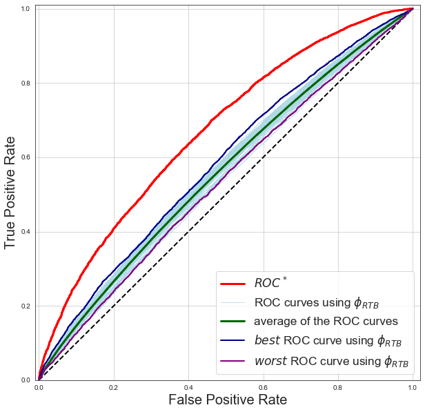
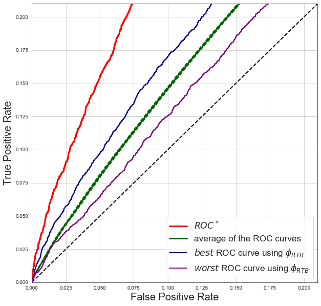
3.c. $\phi_{RTB}(u)=u\mathbb{I}\{u\geq 0.9\}$ 3.c. $\phi_{RTB}(u)=u\mathbb{I}\{u\geq 0.9\}$

Figure 7: Empirical $\rm ROC$ curves and average $\rm ROC$ curve for Scale1 ($\varepsilon=0.70$). Samples are drawn from multivariate Gaussian distributions according to section 5.2, scored with early-stopped GA algorithm’s optimal parameter for the class of scoring functions. Hyperparameters: $u_{0}=0.9$, $q=3$, $B=50$, $T=50$. Parameters for the training set: $n=m=150$; $d=15$; for the testing set: $n=m=10^{6}$; $d=15$. Figures $1,2,3$ correspond resp. to the models MMW, Pol, RTB. Light blue curves are the $B(=50)$ $\rm ROC$ curves that are averaged in green (solid line) with $+/-$ its standard deviation (dashed green lines). The dark blue and purple curves correspond to the best and worst scoring functions in the sense of minimization and maximization of the generalization error among the $B$ curves. The red curve corresponds to $\rm ROC^{*}$.

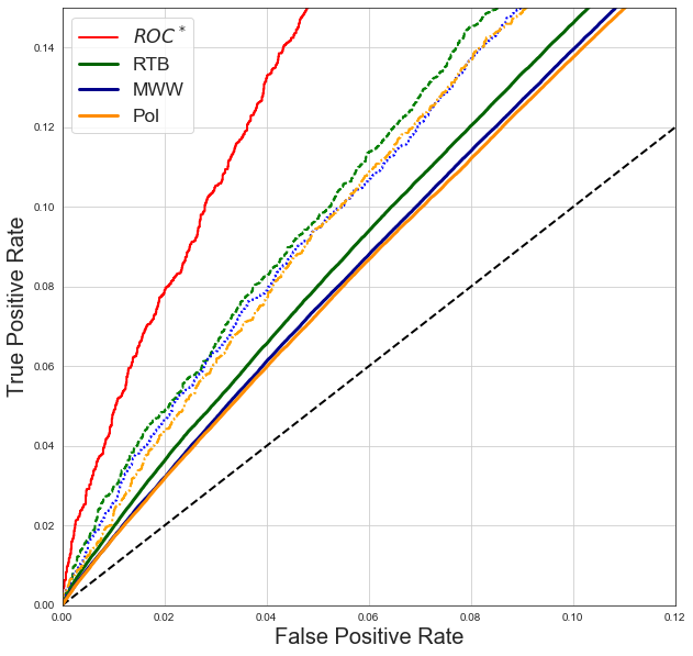
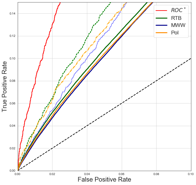
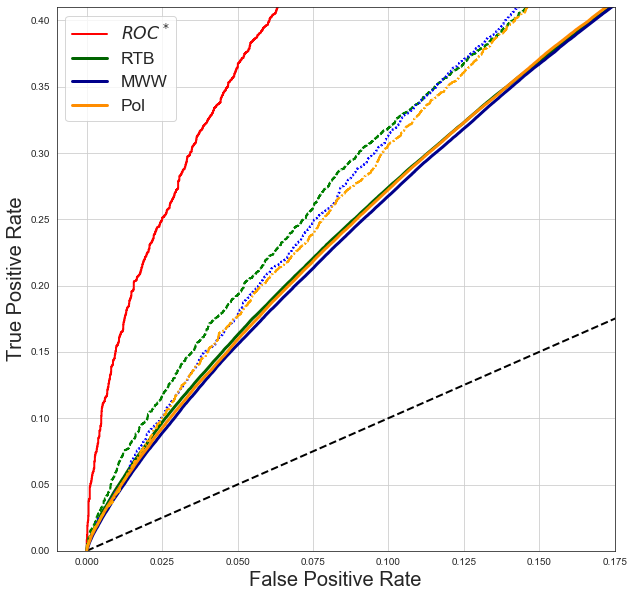
1. Scale1, $\varepsilon=0.70$ 2. Scale2, $\varepsilon=0.90$ 3. Scale3, $\varepsilon=1.10$

Figure 8: Average of the $\rm ROC$ curves (solid line), best $\rm ROC$ curves (dashed line) for the three scale models Scale1, Scale2 and Scale3. In blue for MWW, orange for Pol, green for RTB, red for $\rm ROC^{*}$. Samples are drawn from multivariate Gaussian distributions according to section 5.2, scored with early-stopped GA algorithm’s optimal parameter for the class of scoring functions and averaged after $B=50$ loops. Hyperparameters: $u_{0}=0.9$; $q=3$, $B=50$, $T=50$. Parameters for the training set: $n=m=150$; $d=15$; for the testing set: $n=m=10^{6}$; $d=15$.

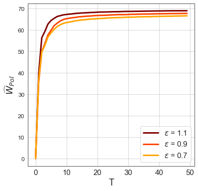
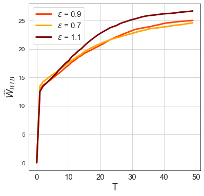
1. $\phi_{MWW}(u)=u$ 2. $\phi_{Pol}(u)=u^{3}$ 3. $\phi_{RTB}(u)=u\mathbb{I}\{u\geq 0.9\}$

Figure 9: Average of the empirical $W_{\phi}$- ranking performance measure over the $B=50$ loops for the three location models Loc1, Loc2 and Loc3. Samples are drawn from multivariate Gaussian distributions according to section 5.2, scored with early-stopped GA algorithm’s optimal parameter for the class of scoring functions and averaged after $B=50$ loops. Hyperparameters: $u_{0}=0.9$; $q=3$, $B=50$, $T=50$. Parameters for the training set: $n=m=150$; $d=15$; for the testing set: $n=m=10^{6}$; $d=15$.

Similar to the location models, the empirical $\rm ROC$ curves over the test pooled samples and additional curves are depicted in Fig. 7, 12, 13 for resp. Scale1, 2 and 3. The averaged $\rm ROC$ curves and the best one are gathered for the three models in Fig. 8. In Fig. 9, the evolution of the averaged empirical value of the $W_{\phi}$-criteria on the train set during the Algorithm is computed. Fig. 15 shows the results for Scale2 for three different parameters of the RTB model with $u_{0}\in\{0.60,\;0.70,\;0.80\}$.

Experimental parameters.

In all the experiments below, the pooled train sample is balanced, i.e. $n=m=150$ and the dimension of the feature space is $d=15$. Similarly for the test sample with $n=m=10^{6}$ and $d=15$. Concerning the score-generating functions, we consider $q=3$ (Pol) and $u_{0}=0.9$ (RTB). We use the Gaussian smoothing kernel $K(u)=(1/\sqrt{2\pi})\exp\{-u^{2}/2\}$ with a bandwidth $h\sim N^{-1/5}$, yielding an (asymptotically) optimal trade-off between bias and variance. Algorithm 1 is implemented with $T=50$ and a learning step size $\eta$ of order $1/\sqrt{T}$. For each model, $B=50$ Monte-Carlo replications of the train pooled sample. Based on the latter, a standard deviation for the test average ROC curve is computed for each model.

Evaluation of the criteria.

In order to evaluate the performance of the scoring function produced by an early-stopped version of Algorithm 1 depending on the score-generating function chosen, it is used to score the test sample and the corresponding $\rm ROC$ curves and its average are compared to those of the optimal scoring function $s_{\theta^{*}}(z)$. Also we consider the best/worst curves in the sense of resp. the minimization/maximization of the generalization error of the set of $\rm ROC$ curves obtained computed over the test pooled sample. Particular attention is paid to the behavior of these curves near the origin, which reflects the ranking performance for the instances with highest score values.

5.3 Results and Discussion

We now analyze the experimental results, by commenting on the test $\rm ROC$ curves obtained after learning the scoring functions, using the early-stopped version of the Algorithm 1 described above, that maximize the chosen (smoothed variant of the) $W_{\phi}$-performance measure: MWW, Pol and RTB. We compare them with $\rm ROC^{*}$. All the experiments were run using Python.

For both the location and scale models, we ran the algorithm for three increasing levels of difficulty defined by the decreasing value of the parameter $\varepsilon$. Figures 5 (location) and 8 (scale) show that the three methods (MWW, Pol, RTB) learn an empirical parameter $\widehat{\theta}_{n,m}$ such that the corresponding $\rm ROC$ curve gets close to $\rm ROC^{*}$ (red curves) and the more $\varepsilon$ increases and the more the scoring rule learned generalizes well. Fig. 6 (location) and 9 (scale) reveal the monotonicity of the evolution of the empirical criteria, as the number of iterative steps of Algorithm 1 increases. Unsurprisingly, all the results show an increasing ability to learn a scoring function that maximizes the three $W_{\phi}$-performance measures, as $\varepsilon$ increases (i.e. when the distribution $G$ and $H$ are significantly more different from each other).

Analyzing the average of the empirical $\rm ROC$ curves obtained, MWW performs better for the location model as its corresponding curve converges faster to $\rm ROC^{*}$ for all $\varepsilon$. This phenomenon was expected due to the well-known high power of the related Mann-Whitney-Wilcoxon test statistic in this modeling. The aggregated $\rm ROC$ curve for the Pol method also performs well, while RTB’s presents a low performance compared to MWW, see Fig. 5. Indeed, considering only the best ranked observations at each iteration in the learning procedure, does not always achieve a good scoring parameter and is enhanced by the early-stopped rule. It results in a higher variance and a larger spectrum of the empirical curves both at the same time, see the light blue curves in Fig. 4.3. and 11.3. (Loc2 and Loc3). The slow convergence for the RTB method is illustrated with Loc1, where almost both samples are blended/coincide, for which only the $\rm ROC$ curves above the diagonal were kept. For the scale model, the aggregated $\rm ROC$ curves are comparable for the three methods with a slightly higher performance obtained by RTB and we note the faster convergence of the algorithm for this model, see Fig. 9.

Looking at the best $\rm ROC$ curves (dark blue lines), defined as those obtained by the scoring function minimizing the generalization error for each criterion, RTB yields to a scoring function that generalizes best for most of the models. In particular, when focussing on the ’best’ instances in the learning procedure, the obtained empirical scoring functions have higher performance at the beginning of the $\rm ROC$ curves, see the zoomed plots. Also, choosing the optimal proportion $1-u_{0}$ of observations to consider for the score-generating function results in different performance measures. Figure 14 gathers the resulting plots for models Loc2 and 3 with $u_{0}$ in $\{0.7,0.9,0.95\}$ while Fig. 15 depicts the scale model 2 with $u_{0}$ in $\{0.6,0.7,0.8\}$ and a higher number of loops $T=70$. Considering the best $\rm ROC$ curves for all models shows that when $u_{0}$ tends to one, the beginning of the curve is accurately learned. Incidentally, note that the proportion of observations considered has to be large enough, so that the optimization algorithm performs well.

1.a. $\phi_{MWW}(u)=u$ 2.b. $\phi_{Pol}(u)=u^{3}$ 1.a. $\phi_{MWW}(u)=u$ 2.b. $\phi_{Pol}(u)=u^{3}$

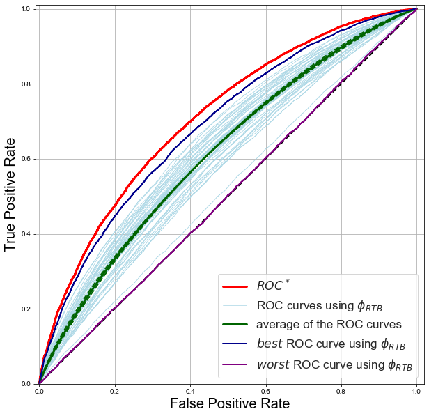
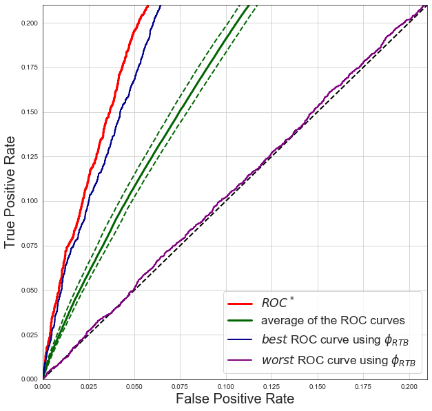
3.c. $\phi_{RTB}(u)=u\mathbb{I}\{u\geq 0.9\}$ 3.c. $\phi_{RTB}(u)=u\mathbb{I}\{u\geq 0.9\}$

Figure 4: Empirical $\rm ROC$ curves and average $\rm ROC$ curve for Loc2 ($\varepsilon=0.20$). Samples are drawn from multivariate Gaussian distributions according to section 5.2, scored with early-stopped GA algorithm’s optimal parameter for the class of scoring functions. Hyperparameters: $u_{0}=0.9$, $q=3$, $B=50$, $T=50$. Parameters for the training set: $n=m=150$; $d=15$; for the testing set: $n=m=10^{6}$; $d=15$. Figures $1,2,3$ correspond resp. to the models MMW, Pol, RTB. Light blue curves are the $B(=50)$ $\rm ROC$ curves that are averaged in green (solid line) with $+/-$ its standard deviation (dashed green lines). The dark blue and purple curves correspond to the best and worst scoring functions in the sense of minimization and maximization of the generalization error among the $B$ curves. The red curve corresponds to $\rm ROC^{*}$.

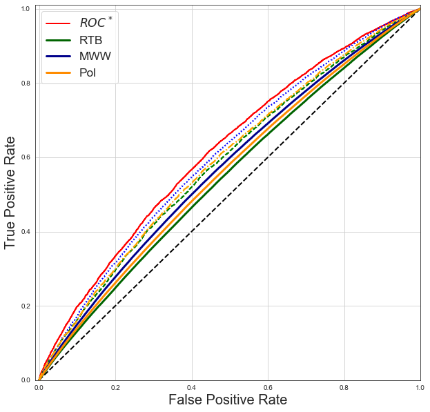
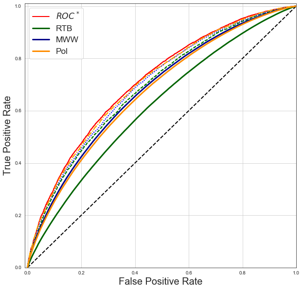
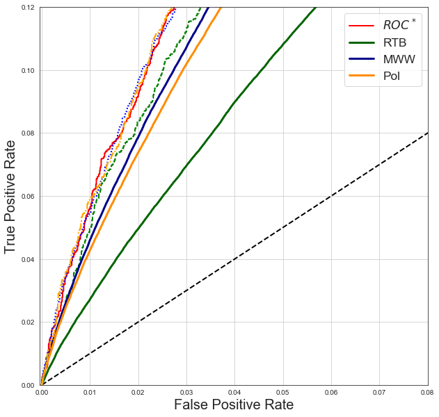
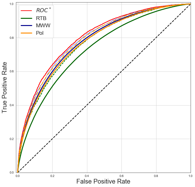
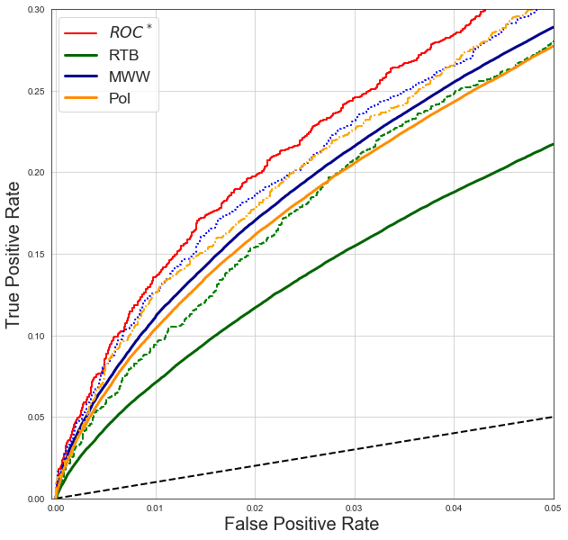
1. Loc1, $\varepsilon=0.10$ 2. Loc2, $\varepsilon=0.20$ 3. Loc3, $\varepsilon=0.30$

Figure 5: Average of the $\rm ROC$ curves (solid line), best $\rm ROC$ curves (dashed line) for the three location models Loc1, Loc2 and Loc3. In blue for MWW, orange for Pol, green for RTB, red for $\rm ROC^{*}$. Samples are drawn from multivariate Gaussian distributions according to section 5.2, scored with early-stopped GA algorithm’s optimal parameter for the class of scoring functions and averaged after $B=50$ loops. Hyperparameters: $u_{0}=0.9$; $q=3$, $B=50$, $T=50$. Parameters for the training set: $n=m=150$; $d=15$; for the testing set: $n=m=10^{6}$; $d=15$.

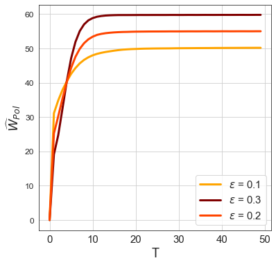
1. $\phi_{MWW}(u)=u$ 2. $\phi_{Pol}(u)=u^{3}$ 3. $\phi_{RTB}(u)=u\mathbb{I}\{u\geq 0.9\}$

Figure 6: Average of the empirical $W_{\phi}$-ranking performance measure over the $B=50$ loops for the three location models Loc1, Loc2 and Loc3. Samples are drawn from multivariate Gaussian distributions according to section 5.2, scored with early-stopped GA algorithm’s optimal parameter for the class of scoring functions and averaged after $B=50$ loops. Hyperparameters: $u_{0}=0.9$; $q=3$, $B=50$, $T=50$. Parameters for the training set: $n=m=150$; $d=15$; for the testing set: $n=m=10^{6}$; $d=15$.

1.a. $\phi_{MWW}(u)=u$ 2.b. $\phi_{Pol}(u)=u^{3}$ 1.a. $\phi_{MWW}(u)=u$ 2.b. $\phi_{Pol}(u)=u^{3}$

6 Conclusion

This article argues that two-sample linear rank statistics provide a very flexible and natural class of empirical performance measures for bipartite ranking. We have showed that it encompasses in particular well-known criteria used in medical diagnosis and information retrieval and proved that, in expectation, these criteria are maximized by optimal scoring functions and put the emphasis on specific parts of their ROC curves, depending on the score generating function involved in the criterion considered. We have established concentration results for collections of such statistics, referred to as two-sample rank processes here, under general assumptions and have deduced from them statistical learning guarantees for the maximizers of such ranking criteria in the form of a generalization bound of order $O_{\mathbb{P}}(1/\sqrt{N})$, where $N$ means the size of the pooled training sample. Algorithmic issues concerning practical maximization have also been investigated and we have displayed numerical results supporting the theoretical analysis carried out.

Appendix A Definitions and Preliminary Results

For the sake of clarity, crucial concepts and results extensively used in the technical analysis subsequently carried out are first recalled.

A.1 Hájek Projection Method

The Hájek projection method introduced in the seminal contribution [18] aims at decomposing (linearizing) any (possibly complex) square integrable statistic based on independent observations, so as to express it as an average of independent r.v.’s plus an uncorrelated term. The proof of Proposition 4 crucially relies on this technique. For completeness, it is described in the following lemma, one may refer to Chapter 11 in [35] for further details.

Lemma. 10.

(Hájek projection, [18]) Let $Z_{1},\;\ldots,\;Z_{n}$ be independent r.v.’s and $T_{n}=T_{n}(Z_{1},\;\ldots,\;Z_{n})$ be a real-valued square integrable statistic. The Hájek projection of $T_{n}$ is defined as $\widehat{T}_{n}=\sum_{i=1}^{n}\mathbb{E}[T_{n}\mid Z_{i}]-(n-1)\mathbb{E}[T]$. It is the orthogonal projection of the square integrable r.v. $T_{n}$ onto the subspace of all variables of the form $\sum_{i=1}^{n}g_{i}(Z_{i})$, for arbitrary measurable functions $g_{i}$ s.t. $\mathbb{E}[g^{2}_{i}(Z_{i})]<+\infty$.

A.2 $U$-statistics and $U$-processes

As mentioned in Section 3, (degenerate) one/two-sample $U$-statistics are involved in the definition of the residual term introduced in Proposition 4. We recall the definition of such statistics generalizing basic i.i.d. sample averages, as well as some of their properties. See e.g. [23] for an account of the theory of $U$-statistics.

Definition. 11.

(One-sample $U$-Statistic of degree two) Let $n\geq 2$. Consider a i.i.d. sequence $X_{1},\;\ldots,\;X_{n}$ drawn from a probability distribution $\mu$ on a measurable space ${\cal X}$ and $k:{\cal X}^{2}\rightarrow\mathbb{R}$ a square integrable function w.r.t. $\mu\otimes\mu$. The one-sample $U$-statistic of degree $2$ and kernel function $k$ based on the $X_{i}$’s is defined as:

$$U_{n}(k)=\frac{1}{n(n-1)}\sum_{1\leq i\neq j\leq n}k(X_{i},X_{j})~{}.$$ (A.1)

As can be shown by a basic Lehmann-Scheffé argument, the statistic $U_{n}(h)$ is the unbiased estimator of the parameter $\theta(k)=\int k(x_{1},\;x_{2})\mu(dx_{1})\mu(dx_{2})$ with minimum variance. Its Hájek projection can be expressed as follows: the projection of $U_{n}(k)-\theta(k)$ onto the space of all random variables $\sum_{i=1}^{n}g_{i}(X_{i})$ with $\int g_{i}^{2}(x)\mu(dx)<+\infty$ is $\widehat{U}_{n}(k)=(1/n)\sum_{i=1}^{n}k_{1}(X_{i})$, with $k_{1}=k_{1,1}+k_{1,2}$, $k_{1,1}(x)=\mathbb{E}[k(X_{1},\;x)]-\theta$ and $k_{1,2}(x)=\mathbb{E}[k(x,\;X_{2})]-\theta$ for all $x\in{\cal X}$. The $U$-statistic (A.1) is said to be degenerate when the $k_{1,l}(X_{1})$’s are equal to zero with probability one, it is then of order $O_{\mathbb{P}}(1/n)$. Hence, once recentered, the $U$-statistic (A.1) can be written as the i.i.d. average $\widehat{U}_{n}(h)$ plus a degenerate $U$-statistic. This decomposition is known as the (second) Hoeffding representation of $U$-statistics and provides the key argument to establish limit results for such functionals, see e.g. [31].

The notion of $U$-statistic can be generalized in several ways, by considering kernels with a number of arguments (i.e. degree) higher than $2$ or by extending it to the multi-sample framework.

Definition. 12.

(Two-sample $U$-Statistic of degree $(1,1)$) Let $n,\;m$ in $\mathbb{N}^{*}$. Consider two independent i.i.d. sequences $X_{1},\;\ldots,\;X_{n}$ and $Y_{1},\;\ldots,\;Y_{m}$ respectively drawn from probability distributions $\mu$ and $\nu$ on the measurable spaces ${\cal X}$ and ${\cal Y}$. Let $\ell:{\cal X}\times{\cal Y}\rightarrow\mathbb{R}$ be a square integrable function w.r.t. $\mu\otimes\nu$. The two-sample $U$-statistic of degree $(1,1)$, with kernel function $\ell(x,y)$ and based on the $X_{i}$’s and the $Y_{j}$’s is defined as:

$$U_{n,m}(\ell)=\frac{1}{nm}\sum_{i=1}^{n}\sum_{j=1}^{m}\ell(X_{i},Y_{j})~{}.$$ (A.2)

A classic example of two-sample $U$-statistic of degree $(1,1)$ is the Mann-Whitney statistic, with symmetric kernel $\ell(x,y)=\mathbb{I}\{y<x\}+(1/2)\mathbb{I}\{y=x\}$ on $\mathbb{R}^{2}$ and degree $(1,1)$. It is a natural (unbiased) estimator of the $\rm AUC$: when computed from univariate samples $X_{1},\;\ldots,\;X_{n}$ and $Y_{1},\;\ldots,\;Y_{m}$ with distributions $H$ and $G$ on $\mathbb{R}$, it is equal to $\rm AUC_{\widehat{H}_{m},\widehat{G}_{n}}$ with the notations of Subsection 2.2 and can be thus viewed as an affine transform of the rank-sum Wilcoxon statistic (2.9).
The Hájek projection of (A.2) is obtained by computing the orthogonal projection of the recentered r.v. $U_{n,m}(\ell)-\mathbb{E}[U_{n,m}(\ell)]$ onto the subpace of $L_{2}$ composed of all random variables $\sum_{i=1}^{n}g_{i}(X_{i})+\sum_{j=1}^{m}f_{j}(Y_{j})$ with $\int g_{i}^{2}(x)\mu(dx)<+\infty$ and $\int f_{j}^{2}(y)\nu(dy)<+\infty$, namely $\widehat{U}_{n,m}(\ell)=(1/n)\sum_{i=1}^{n}\ell_{1,1}(X_{i})+(1/m)\sum_{j=1}^{m}\ell_{1,2}(Y_{j})$, with $\ell_{1,1}(x)=\mathbb{E}[\ell(x,\;Y_{1})]-\mathbb{E}[U_{n,m}(\ell)]$ and $\ell_{1,2}(y)=\mathbb{E}[\ell(X_{1},\;y)]-\mathbb{E}[U_{n,m}(\ell)]$ for all $(x,y)\in{\cal X}\times{\cal Y}$. The $U$-statistic $U_{n,m}(\ell)$ is said to be degenerate when the random variables $\ell_{1,1}(X_{1})$ and $\ell_{1,2}(Y_{1})$ are equal to zero with probability one. Similar to (A.1), the recentered version of the two-sample $U$-statistic of degree $(1,1)$ (A.2) can be written as a sum of two i.i.d. averages $\widehat{U}_{n,m}(\ell)$ plus a degenerate $U$-statistic of order $O_{\mathbb{P}}(1/n)+O_{\mathbb{P}}(1/m)$. Again, the Hoeffding decomposition is the key to directly extend limit results known for i.i.d. averages (e.g. SLLN, CLT, LIL) to statistics of the type (A.2). In the subsequent technical analysis, nonasymptotic uniform results are required for $U$-processes, namely collections of $U$-statistics indexed by classes of kernels. By means of the Hoeffding decomposition, concentration bounds for $U$-processes can be obtained by combining classic concentration bounds for empirical processes and concentration bounds for degenerate $U$-processes, such as those recalled in A.4.

A.3 ${\sc VC}$-type Classes of Functions - Permanence Properties

The concentration inequalities for $U$-processes recalled in Appendix A.4 and involved in the proof of the main results stated in this article apply to collections of kernels that are of VC-type, a classic concept used to quantify the complexity of classes of functions. It is recalled below, see e.g. [36] for generalizations and further details.

Definition. 13.

A class $\mathcal{F}$ of real-valued functions defined on a measurable space ${\cal Z}$ is a bounded ${\sc VC}$-type class with parameter $(A,{\cal V})\in(0,\;+\infty)^{2}$ and constant envelope $L_{\mathcal{F}}>0$ if for all $\varepsilon\in(0,1)$:

$$\underset{Q}{\sup}\;N(\mathcal{F},L_{2}(Q),\varepsilon L_{\mathcal{F}})\leq\left(\frac{A}{\varepsilon}\right)^{{\cal V}}~{},$$ (A.3)

where the supremum is taken over all probability measures $Q$ on ${\cal Z}$ and the smallest number of $L_{2}(Q)$-balls of radius less than $\varepsilon$ required to cover class $\mathcal{F}$ (i.e. covering number) is meant by $N(\mathcal{F},L_{2}(Q),\varepsilon)$.

Recall that a bounded VC class of functions with VC dimension $V<+\infty$ is of VC-type and fulfills the condition above with ${\cal V}=2(V-1)$ and $A=(cV(16e)^{V})^{1/(2(V-1))}$, where $c$ is a universal constant, see e.g. Theorem 2.6.7 in [36]. The lemma stated below permits to control the complexity of the classes of kernels/functions involved in the Hoeffding decompositions of a two-sample $U$-process of degree $(1,1)$ or of a one-sample $U$-process of degree $2$, cf subsection A.2.

Lemma. 14.

Let $X$ and $Y$ be two independent random variables, valued in ${\cal X}$ and ${\cal Y}$ respectively, with probability distributions $\mu$ and $\nu$. Consider $\mathcal{L}$ a VC-type bounded class of kernels $\ell:{\cal X}\times{\cal Y}\rightarrow\mathbb{R}$ with parameters $(A,{\cal V})$ and constant envelope $L_{\mathcal{L}}>0$. Then, the sets of functions $\{x\in{\cal X}\mapsto\mathbb{E}[\ell(x,\;Y)]:\;\ell\in\mathcal{L}\}$, $\{y\in{\cal Y}\mapsto\mathbb{E}[\ell(X,\;y)]:\;\ell\in\mathcal{L}\}$, $\{\ell(x,y)-\mathbb{E}[\ell(X,\;y)]-\mathbb{E}[\ell(x,\;Y)]:\;\ell\in\mathcal{L}\}$ are also VC-type bounded classes.

proof. Consider first the uniformly bounded class $\mathcal{L}_{1}$ composed of functions $x\in{\cal X}\mapsto\mathbb{E}[\ell(x,\;Y)]$ with $\ell\in\mathcal{L}$. Let $\varepsilon>0$ and $P$ be any probability measure on ${\cal X}$. Define the probability measure $P_{\nu}(dx,dy)=P(dx)\nu(dy)$ on ${\cal X}\times{\cal Y}$ and consider a $\varepsilon$-covering of the class $\mathcal{L}$ with centers $\ell_{1},\ldots,\;\ell_{K}$ w.r.t. the metric $L_{2}(P_{\nu})$, $K\geq 1$. For all $\ell\in\mathcal{L}$, there exists $k\leq K$ such that:

$$\int_{x\in{\cal X}}\int_{y\in{\cal Y}}(\ell(x,\;y)-\ell_{k}(x,\;y))^{2}P_{\nu}(dx,dy)\leq\varepsilon^{2}~{}.$$

By virtue of Jensen’s inequality, we have

$$\int_{{\cal X}}(\mathbb{E}[\ell(x,\;Y)]-\mathbb{E}[\ell_{k}(x,\;Y)])^{2}P(dx)\\ \leq\int_{{\cal X}}\mathbb{E}[(\ell(x,\;Y)-\ell_{k}(x,\;Y))^{2}]P(dx)\\ =\int_{{\cal X}}\int_{{\cal Y}}(\ell(x,\;y)-\ell_{k}(x,\;y))^{2}\nu(dy)P(dx)\leq\varepsilon^{2}~{}.$$

Hence, one gets a $\varepsilon$-covering of the class $\mathcal{L}_{1}$ with balls of centers $\{\mathbb{E}[\ell_{k}(\cdot,\;Y)]:\;k=1,\;\ldots,\;K\}$ in $L_{2}(P)$. This proves that

$$N({\cal L}_{1},L_{2}(P),\varepsilon L_{\mathcal{L}})\leq N({\cal L},L_{2}(P_{\nu}),\varepsilon L_{\mathcal{L}}).$$

As a similar reasoning can be applied to the two other classes of functions, one then gets the desired result.

A.4 Concentration Inequalities for Degenerate $U$-processes.

In [24] (see Theorem 2 therein), a concentration bound for one-sample degenerate $U$-processes of arbitrary degree indexed by $L_{2}$-dense classes of non-symmetric kernels is established. The lemma below is a formulation of the latter in the specific case of degenerate $U$-processes of degree $2$ indexed by VC-type bounded classes of non-symmetric kernels.

Lemma. 15.

Let $n\geq 2$ and $X_{1},\;\ldots,\;X_{n}$ be i.i.d. random variables drawn from a probability distribution $\mu$ on a measurable space ${\cal X}$. Let $\mathcal{K}$ be a class of measurable kernels $k:{\cal X}^{2}\rightarrow\mathbb{R}$ such that $\sup_{x,x^{\prime}\in{\cal X}^{2}}|k(x,x^{\prime})|\leq D<+\infty$ and $\int_{{\cal X}^{2}}k^{2}(x,x^{\prime})\mu(dx)\mu(dx^{\prime})\leq\sigma^{2}\leq D^{2}$, that defines a degenerate one-sample $U$-process of degree $2$, based on the $X_{i}$’s: $\{U_{n}(k)\>\;k\in\mathcal{K}\}$. Suppose in addition that the class $\mathcal{K}$ is of VC-type with parameters $(A,{\cal V})$. Then, there exist constants $C_{1}>0,\;C_{2}\geq 1$ and $C_{3}\geq 0$ depending on $(A,{\cal V})$ such that:

$$\mathbb{P}\left\{\sup_{k\in\mathcal{K}}\left|U_{n}(k)\right|\geq t\right\}\leq C_{2}\exp\left\{-\frac{C_{3}(n-1)t}{\sigma}\right\}~{},$$ (A.4)

as soon as $C_{1}\log(2D/\sigma)\leq(n-1)t/\sigma\leq n\sigma^{2}/D^{2}$.

The next lemma provides a similar nonasymptotic result for degenerate two-sample $U$-processes of degree $(1,1)$.

Lemma. 16.

Let $(n,\;m)\in\mathbb{N}^{*}$. Consider two independent i.i.d. random samples $X_{1},\ldots,X_{n}$ and $Y_{1},\ldots,Y_{m}$ respectively drawn from the probability distributions $\mu$ and $\nu$ on the measurable spaces ${\cal X}$ and ${\cal Y}$. Let ${\cal L}$ be a class of degenerate non-symmetrical kernels $\ell:{\cal X}\times{\cal Y}\to\mathbb{R}$ such that $\sup_{(x,y)\in{\cal X}\times{\cal Y}}|\ell(x,y)|\leq L<+\infty$ and $\int_{{\cal X}\times{\cal Y}}\ell^{2}(x,y)\mu(dx)\nu(dy)\leq\sigma^{2}\leq L^{2}$, that defines a degenerate two-sample $U$-process of degree $(1,1)$, based on the $X_{i},Y_{j}$’s: $\{U_{n,m}(\ell)\>\;\ell\in{\cal L}\}$. Suppose in addition that the class ${\cal L}$ is of VC-type with parameters $(A,{\cal V})$. Then, for all $t>0$, there exists a universal constant $K>2$ such that:

$$\mathbb{P}\left\{\sup_{\ell\in{\cal L}}|U_{n,m}(\ell)|\geq t\right\}\leq K2^{{\cal V}}(A/L)^{2{\cal V}}e^{4/L^{2}}\exp\left\{-\frac{nmt^{2}}{ML^{2}}\right\}~{},$$ (A.5)

for all $nmt^{2}>\max(8^{4}\log(2)L^{2}{\cal V},(\log(2)L^{2}{\cal V}/2)^{1+\delta})$, $\delta\in(1,2)$ constant and $M=16^{3}/2$.

Its proof is given in B.7 and is inspired from that of Lemma 2.14.9 in [36] and of Lemma 3.2 in [34] for empirical processes, and from Lemma 2.4 in [28] which gives a version in expectation applicable to degenerate two-sample $U$-processes of arbitrary degree indexed by $L_{p}$-dense classes of kernels.

Appendix B Technical Proofs

The proofs of the results stated in the paper are detailed below.

B.1 Proof of Proposition 4

Let $\theta_{0}\in(0,1)$. Since $\phi(u)\in\mathcal{C}^{2}([0,1],\mathbb{R})$ by virtue of Assumption 2, a Taylor expansion of order two yields: for all $\theta\in(0,1)$

$$\phi(\theta)=\phi(\theta_{0})+(\theta-\theta_{0})\phi^{\prime}(\theta_{0})+\int_{\theta_{0}}^{\theta}(\theta-u)\phi^{\prime\prime}(u)du~{}.$$ (B.1)

Let $s\in{\cal S}_{0}$. For all $t\in\mathbb{R}$, we have

$$\phi\left(\frac{N\widehat{F}_{s,N}(t)}{N+1}\right)=\phi\circ F_{s}(t)+\left(\frac{N\widehat{F}_{s,N}(t)}{N+1}-F_{s}(t)\right)\phi^{\prime}\circ F_{s}(t)\\ +\int_{F_{s}(t)}^{N\widehat{F}_{s,N}(t)/(N+1)}\left(\frac{N\widehat{F}_{s,N}(t)}{N+1}-u\right)\phi^{\prime\prime}(u)du~{},$$ (B.2)

with probability one. Let $i\leq n$, for $t=s(\mathbf{X}_{i})$, (B.2) writes:

$$\phi\left(\frac{N\widehat{F}_{s,N}(s(\mathbf{X}_{i}))}{N+1}\right)=\phi\circ F_{s}(s(\mathbf{X}_{i}))\\ +\left(\frac{N\widehat{F}_{s,N}(s(\mathbf{X}_{i}))}{N+1}-F_{s}(s(\mathbf{X}_{i}))\right)\phi^{\prime}\circ F_{s}(s(\mathbf{X}_{i}))+t_{i}(s)\quad a.s.~{},$$ (B.3)

where

$$|t_{i}(s)|\leq(\|\phi^{\prime\prime}\|_{\infty}/2)\left(N/(N+1)\widehat{F}_{s,N}(s(\mathbf{X}_{i}))-F_{s}(s(\mathbf{X}_{i}))\right)^{2}.$$

Hence, by summing over $i\in\{1,\;\ldots,\;n\}$, one gets that the approximation of $\widehat{W}_{n,m}(s)$ stated below holds true almost-surely:

$$\widehat{W}_{n,m}(s)=n\widehat{W}_{\phi}(s)+B_{n,m}(s)+\widehat{T}_{n,m}(s)~{},$$ (B.4)

where

$$B_{n,m}(s) = \sum_{i=1}^{n}\left(\frac{N\widehat{F}_{s,N}(s(\mathbf{X}_{i}))}{N+1}-F_{s}(s(\mathbf{X}_{i}))\right)\phi^{\prime}\circ F_{s}(s(\mathbf{X}_{i})),$$ (B.5)

$$|\widehat{T}_{n,m}(s)| = \sum_{i=1}^{n}|t_{i}(s)|\leq\frac{\|\phi^{\prime\prime}\|_{\infty}}{2}\sum_{i=1}^{n}\left(\frac{N\widehat{F}_{s,N}(s(\mathbf{X}_{i}))}{N+1}-F_{s}(s(\mathbf{X}_{i}))\right)^{2}~{}.$$ (B.6)

Linearization of $B_{n,m}(\cdot)$.

First, observe that

$$B_{n,m}(s)=\frac{1}{N+1}\sum_{i=1}^{n}\sum_{j\neq i}^{n}\mathbb{I}\{s(\mathbf{X}_{j})\leq s(\mathbf{X}_{i})\}\phi^{\prime}\circ F_{s}(s(\mathbf{X}_{i}))\\ +\frac{1}{N+1}\sum_{i=1}^{n}\sum_{j=1}^{m}\mathbb{I}\{s(\mathbf{Y}_{j})\leq s(\mathbf{X}_{i})\}\phi^{\prime}\circ F_{s}(s(\mathbf{X}_{i}))\\ +\sum_{i=1}^{n}\left(\frac{1}{N+1}-F_{s}(s(\mathbf{X}_{i}))\right)\phi^{\prime}\circ F_{s}(s(\mathbf{X}_{i}))~{}.$$ (B.7)

Notice that the first two terms are $U$-processes indexed by ${\cal S}_{0}$, cf Section A.2, while the last term is an empirical process. Indeed, one may write

$$B_{n,m}(s)=\frac{n(n-1)}{N+1}U_{n}(k_{s})+\frac{nm}{N+1}U_{n,m}(\ell_{s})+\widehat{K}_{n,m}(s)~{},$$ (B.8)

where

$$U_{n}(k_{s})=\frac{1}{n(n-1)}\sum_{i=1}^{n}\sum_{j\neq i}^{n}\mathbb{I}\{s(\mathbf{X}_{j})\leq s(\mathbf{X}_{i})\}\phi^{\prime}\circ F_{s}(s(\mathbf{X}_{i}))$$ (B.9)

is a (nondegenerate) $1$-sample $U$-process of degree $2$ based on the random sample $\{\mathbf{X}_{1},\;\ldots,\;\mathbf{X}_{n}\}$ with nonsymmetric kernel $k_{s}(x,x^{\prime})=\mathbb{I}\{s(x^{\prime})\leq s(x)\}\phi^{\prime}\circ F_{s}(s(x))$ on ${\cal X}\times{\cal X}$,

$$U_{n,m}(\ell_{s})=\frac{1}{nm}\sum_{i=1}^{n}\sum_{j=1}^{m}\mathbb{I}\{s(\mathbf{Y}_{j})\leq s(\mathbf{X}_{i})\}\phi^{\prime}\circ F_{s}(s(\mathbf{X}_{i}))$$ (B.10)

is a (nondegenerate) two-sample $U$-process of degree $(1,1)$ based on the samples $\{\mathbf{X}_{1},\;\ldots,\;\mathbf{X}_{n}\}$ and $\{\mathbf{Y}_{1},\;\ldots,\;\mathbf{Y}_{m}\}$ with kernel $\ell_{s}(x,y)=\mathbb{I}\{s(y)\leq s(x)\}\phi^{\prime}\circ F_{s}(s(x))$ on ${\cal X}\times{\cal Y}$, and

$$\widehat{K}_{n,m}(s)=\sum_{i=1}^{n}\left(\frac{1}{N+1}-F_{s}(s(\mathbf{X}_{i}))\right)\phi^{\prime}\circ F_{s}(s(\mathbf{X}_{i}))$$

is an empirical process based on the $\mathbf{X}_{i}$’s. In order to write $B_{n,m}$ as an empirical process plus a (negligible) remainder term, the Hoeffding decomposition is applied to the $U$-processes above, cf Appendix A.2:

$$U_{n}(k_{s}) = \mathbb{E}[U_{n}(k_{s})]+\widehat{U}_{n}(k_{s})+\mathcal{R}_{n}(k_{s})~{},$$ (B.11)

$$U_{n,m}(\ell_{s}) = \mathbb{E}[U_{n,m}(\ell_{s})]+\widehat{U}_{n,m}(\ell_{s})+\mathcal{R}_{n,m}(\ell_{s})~{},$$ (B.12)

where

$$\widehat{U}_{n}(k_{s})=\frac{1}{n}\sum_{i=1}^{n}k_{s,1,1}(\mathbf{X}_{i})+\frac{1}{n}\sum_{i=1}^{n}k_{s,1,2}(\mathbf{X}_{i})~{},$$ (B.13)

with $k_{s,1,1}(x)=\mathbb{E}[k_{s}(x,\mathbf{X})]-\mathbb{E}[U_{n}(k_{s})]$ and $k_{s,1,2}(x)=\mathbb{E}[k_{s}(\mathbf{X},x)]-\mathbb{E}[U_{n}(k_{s})]$, and

$$\widehat{U}_{n,m}(\ell_{s})=\frac{1}{m}\sum_{j=1}^{m}\ell_{s,1,1}(\mathbf{Y}_{j})+\frac{1}{n}\sum_{i=1}^{n}\ell_{s,1,2}(\mathbf{X}_{i})~{},$$ (B.14)

with $\ell_{s,1,1}(y)=\mathbb{E}[\ell_{s}(\mathbf{X},y)]-\mathbb{E}[U_{n,m}(\ell_{s})]$ and $\ell_{s,1,2}(x)=\mathbb{E}[\ell_{s}(x,\mathbf{Y})]-\mathbb{E}[U_{n,m}(\ell_{s})]$.

Consequently, the Hájek projection of the process $B_{n,m}(s)$ is given by

$$\widehat{B}_{n,m}(s)-\mathbb{E}[\widehat{B}_{n,m}(s)]=\frac{n(n-1)}{N+1}\widehat{U}_{n}(k_{s})+\frac{nm}{N+1}\widehat{U}_{n,m}(\ell_{s})+\widehat{K}_{n,m}(s)-\mathbb{E}[\widehat{K}_{n,m}(s)]~{}.$$ (B.15)

The following result provides an approximation of (B.15) and is proved in Appendix B.2.2.

Lemma. 17.

Under Assumptions 1-3, the Hájek projection of the stochastic process $B_{n,m}(\cdot)$, denoted by $\widehat{B}_{n,m}(\cdot)$ and indexed by ${\cal S}_{0}$, onto the subspace generated by the random variables $\mathbf{X}_{1},\;\ldots,\;\mathbf{X}_{n}$ and $\mathbf{Y}_{1},\;\ldots,\;\mathbf{Y}_{m}$ can be approximated as follows: for all $s\in{\cal S}_{0}$,

$$\widehat{B}_{n,m}(s)-\mathbb{E}\left[\widehat{B}_{n,m}(s)\right]=\widehat{V}_{n}^{X}(s)+\widehat{V}_{m}^{Y}(s)+\widehat{R}_{n,m}(s)~{},$$ (B.16)

where

$$\widehat{V}_{n}^{X}(s)=\frac{n-1}{N+1}\sum_{i=1}^{n}k_{s,1,1}(\mathbf{X}_{i}),\;\widehat{V}_{m}^{Y}(s)=\frac{n}{N+1}\sum_{j=1}^{m}\ell_{s,1,1}(\mathbf{Y}_{j})~{}.$$

Let $\delta>0$, there exist constants $A_{1}>0,\;A_{2}\geq 2$ depending on $\phi$ and ${\cal V}$ such that for all $A_{4}\geq A_{1}$ and $A_{3}=(1/4A_{4}A_{2})\log(1+A_{4}/(4A_{2}))$

$$\mathbb{P}\left\{\sup_{s\in{\cal S}_{0}}\bigg{|}\widehat{R}_{n,m}(s)\bigg{|}>t\right\}\leq A_{2}\exp\left\{-\frac{A_{3}Nt^{2}}{p\sigma^{2}}\right\}~{},$$ (B.17)

as soon as $2A_{1}\sigma\sqrt{p\log(2\|\phi^{\prime}\|_{\infty}/\sigma)/N}\leq t\leq 2pA_{4}\|\phi^{\prime}\|_{\infty}$, with $\sigma^{2}=\int_{[0,1]}\phi^{\prime 2}$.

The last step relies on all previous decompositions, so as to approximate $B_{n,m}(\cdot)$ by the sum of two empirical processes $\widehat{V}_{n}^{X}(\cdot)$ and $\widehat{V}_{n}^{Y}(\cdot)$, with a uniform control of the error. All residual terms, $\widehat{R}_{n,m}(s)$ (Lemma 17) plus the remainders of the $U$-processes, are the components of the process $\mathcal{R}_{n,m}^{B}(s)$ , see the following Lemma 18.

Lemma. 18.

Suppose that Assumptions 1-3 are fulfilled. The stochastic process $B_{n,m}(.)$ can be approximated as follows: for all $s\in{\cal S}_{0}$,

$$B_{n,m}(s)-\mathbb{E}\left[B_{n,m}(s)\right]=\widehat{V}_{n}^{X}(s)+\widehat{V}_{m}^{Y}(s)+\mathcal{R}_{n,m}^{B}(s)~{}.$$ (B.18)

Let $\delta>0$. There exist $D_{1}>0$ universal constant, and constants $D_{3},\;D_{4}>0,\;D_{2}\geq 1$, $d_{1},\;d_{2}>3$ depending on $\phi$ and ${\cal V}$, such that with probability at least $1-\delta$:

$$\sup_{s\in{\cal S}_{0}}|\mathcal{R}_{n,m}^{B}(s)|\leq\|\phi^{\prime}\|_{\infty}\sqrt{p(1-p)D_{1}\log(d_{1}/\delta)}+(p\|\phi^{\prime}\|_{\infty}D_{4})\log(d_{2}/\delta)~{},$$ (B.19)

as soon as $N\geq(pD_{3})^{-1}\log(D_{2}/\delta)$.

Refer to Appendix B.2.3 for the detailed proof.

A uniform bound for $\widehat{T}_{n,m}(\cdot)$.

By virtue of (B.5), we have:

$$\sup_{s\in{\cal S}_{0}}|\widehat{T}_{n,m}(s)|\leq n\|\phi^{\prime\prime}\|_{\infty}\left(\sup_{(s,t)\in{\cal S}_{0}\times\mathbb{R}}\left(\widehat{F}_{s,N}(t)-F_{s}(t)\right)^{2}+\frac{1}{(N+1)^{2}}\right).$$ (B.20)

Observe also that

$$\sup_{(s,t)\in{\cal S}_{0}\times\mathbb{R}}|\widehat{F}_{s,N}(t)-F_{s}(t)|\leq p\sup_{(s,t)\in{\cal S}_{0}\times\mathbb{R}}|\widehat{G}_{s,n}(t)-G_{s}(t)|\\ +(1-p)\sup_{(s,t)\in{\cal S}_{0}\times\mathbb{R}}|\widehat{H}_{s,m}(t)-H_{s}(t)|+\frac{2}{N}~{}.$$ (B.21)

A classic concentration bound for empirical processes based on the VC inequality (see e.g. Theorems 3.2 and 3.4 in [2]) shows that, for any $\delta\in(0,1)$, we have with probability at least $1-\delta$:

$$\sup_{(s,t)\in{\cal S}_{0}\times\mathbb{R}}|\widehat{G}_{s,n}(t)-G_{s}(t)|\leq c\sqrt{\frac{{\cal V}}{n}}+\sqrt{\frac{2\log(1/\delta)}{n}}~{},$$

where $c>0$ is a universal constant. In a similar fashion, we have, with probability larger than $1-\delta$,

$$\sup_{(s,t)\in{\cal S}_{0}\times\mathbb{R}}|\widehat{H}_{s,m}(t)-H_{s}(t)|\leq c\sqrt{\frac{{\cal V}}{m}}+\sqrt{\frac{2\log(1/\delta)}{m}}~{}.$$

Combining the bounds above with the union bound, (B.21) and (B.20) we obtain that, for any $\delta\in(0,1)$, we have with probability larger than $1-\delta$:

$$\sup_{s\in{\cal S}_{0}}|\widehat{T}_{n,m}(s)|\leq n||\phi^{\prime\prime}||_{\infty}\left(12\left(\frac{c^{2}{\cal V}+\log(2/\delta)}{N}+\frac{1}{N^{2}}\right)+\frac{1}{(N+1)^{2}}\right)\\ \leq B_{1}+B_{2}\log(2/\delta)~{},$$ (B.22)

where $B_{1}$ (resp. $B_{2}$) is a constant that only depends on $\phi$ and ${\cal V}$ (resp. on $\phi$).

To end the proof, it suffices to observe that the remainder process is the sum of $\mathcal{R}_{n,m}^{B}(s)$ and $\widehat{T}_{n,m}(s)$. Combining bounds (B.19) and (B.22), we get that, with probability at least $1-\delta$,

$$\sup_{s\in{\cal S}_{0}}|\mathcal{R}_{n,m}(s)|=\sup_{s\in{\cal S}_{0}}|\mathcal{R}_{n,m}^{B}(s)+\widehat{T}_{n,m}(s)|\leq B_{1}+\|\phi^{\prime}\|_{\infty}\kappa_{p}D\log(2d/\delta)+B_{2}\log(4/\delta)$$ (B.23)

as soon as $N\geq(pD_{3})^{-1}\log(D_{2}/\delta)$, with $D=\max(\sqrt{D_{1}},D_{4})$, $d=\max(d_{1},d_{2})$, $\kappa_{p}=\max(\sqrt{p(1-p)},p)$. As $B_{2}>1$ , $d\geq 3$, and for small $\delta$, we obtain the upperbound $B_{1}+(\|\phi^{\prime}\|_{\infty}\kappa_{p}D+B_{2})\log(2d/\delta)$.

B.2 Intermediary Results

The intermediary results involved in Section B.1 are now established.

B.2.1 Permanence Properties

The lemmas below claim that the collections of kernels/functions involved in the decomposition obtained in Appendix B.1 are of VC-type and uniformly bounded.

Lemma. 19.

Suppose that Assumptions 2 and 3 are fulfilled. Then, the collections of kernels $\{k_{s}(x,x^{\prime}):\;s\in{\cal S}_{0}\}$ and $\{\ell_{s}(x,y):\;s\in{\cal S}_{0}\}$ and are bounded VC-type classes of functions with parameters fully determined by ${\cal V}$ and $\phi$.

proof. Recall that: $\forall(x,x^{\prime})\in{\cal X}^{2}$,

$$k_{s}(x,x^{\prime})=\mathbb{I}\{s(x^{\prime})\leq s(x)\}\left(\phi^{\prime}\circ F_{s}\right)(s(x)).$$

Hence, we have $\sup_{(x,x^{\prime})\in{\cal X}^{2}}|k_{s}(x,x^{\prime})|\leq||\phi^{\prime}||_{\infty}$ for all $s\in{\cal S}_{0}$. In additions, since the collections $\{(x,x^{\prime})\in{\cal X}^{2}\mapsto s(x):\;s\in{\cal S}_{0}\}$ and $\{(x,x^{\prime})\in{\cal X}^{2}\mapsto s(x^{\prime}):\;s\in{\cal S}_{0}\}$ are VC classes of functions, classic permanence properties of VC classes of functions (see e.g. Lemma 2.6.18) shows that $\{(x,x^{\prime})\in{\cal X}^{2}\mapsto s(x)-s(x^{\prime}):\;s\in{\cal S}_{0}\}$ is also a VC class, as well as the class of indicator functions $\{(x,x^{\prime})\in{\cal X}^{2}\mapsto\mathbb{I}\{s(x^{\prime})\leq s(x)\}:\;s\in{\cal S}_{0}\}$. Consequently, the argument of Lemma 14’s proof permits to see easily that $\{(x,x^{\prime})\in{\cal X}^{2}\mapsto F_{s}(s(x))=\mathbb{E}[\mathbb{I}\{s(X)\leq s(x)\}]:\;s\in{\cal S}_{0}\}$ is of VC type, just like $\{(x,x^{\prime})\in{\cal X}^{2}\mapsto(\phi^{\prime}\circ F_{s})(s(x)):\;s\in{\cal S}_{0}\}$ using the Lipschitz property of $\phi^{\prime}$, cf Assumption 2. Finally, being composed of products of a function in the bounded VC-type class $\{(x,x^{\prime})\in{\cal X}^{2}\mapsto\mathbb{I}\{s(x^{\prime})\leq s(x)\}:\;s\in{\cal S}_{0}\}$ by a function in the bounded VC-type class $\{(x,x^{\prime})\in{\cal X}^{2}\mapsto(\phi^{\prime}\circ F_{s})(s(x)):\;s\in{\cal S}_{0}\}$, the collection $\{k_{s}:\;s\in{\cal S}_{0}\}$ is still a bounded VC-type class of functions. A similar reasoning can be applied to show that $\{\ell_{s}:\;s\in{\cal S}_{0}\}$ is a bounded VC-type class of kernels on ${\cal X}\times{\cal Y}$.

The following result is straightforwardly deduced from the lemma above combined with Lemma 14.

Lemma. 20.

Suppose that Assumptions 2 and 3 are fulfilled. Then, the collections of functions/kernels $\{k_{s,1,1}(x):\;s\in{\cal S}_{0}\}$, $\{k_{s,1,2}(x):\;s\in{\cal S}_{0}\}$, $\{k_{s}(x,x^{\prime})-k_{s,1,1}(x)-k_{s,1,2}(x^{\prime}):\;s\in{\cal S}_{0}\}$, $\{\ell_{s,1,1}(y):\;s\in{\cal S}_{0}\}$, $\{\ell_{s,1,2}(x):\;s\in{\cal S}_{0}\}$ and $\{\ell_{s}(x,y)-\ell_{s,1,1}(y)-\ell_{s,1,2}(x):\;s\in{\cal S}_{0}\}$ are bounded VC-type classes with parameters fully determined by ${\cal V}$ and $\phi$.

B.2.2 Proof of Lemma 17

For $s\in{\cal S}_{0}$, by adding the diagonal term, the empirical process can be written

$$\widehat{R}_{n,m}(s)=\left(\frac{n}{N+1}-p\right)\sum_{i=1}^{n}k_{s,1,2}(\mathbf{X}_{i})+\left(\frac{m}{N+1}-(1-p)\right)\sum_{i=1}^{n}\ell_{s,1,2}(\mathbf{X}_{i})~{}.$$ (B.24)

We uniformly bound all three empirical processes in probability using classic concentration bounds, see e.g. Theorem 2.1 in [13], as follows. Assuming Assumptions 2-3, Lemma 20 states that each class of functions $\{k_{s,1,2}:s\in{\cal S}_{0}\}$, $\{\ell_{s,1,2}:s\in{\cal S}_{0}\}$ is uniformly bounded and VC-type of parameters depending only on $\phi$ and on the VC dimension ${\cal V}$. For the class $\{x\mapsto\phi^{\prime}\circ F_{s}(s(x)):\;s\in{\cal S}_{0}\}$, the arguments are exposed in the proof of Lemma 19. The variance of the kernels can be bounded for all $s\in{\cal S}_{0}$, by $\sigma^{2}=\int_{[0,1]}\phi^{\prime 2}$ and $\sigma^{2}\leq||\phi^{\prime}||_{\infty}^{2}$ and notice that $|n/(N+1)-p|\leq 1/N$ and $|m/(N+1)-(1-p)|\leq 1/N$. Let $t>0$, there exist a sequence of constants $A_{1,i}>0,A_{2,i}\geq 1$ depending on $\phi$ and ${\cal V}$, $i\in\{1,2\}$, such that for all $A_{4,i}\geq A_{1,i}$ and and $A_{3,i}=(1/A_{4,i}A_{2,i})\log(1+A_{4,i}/(4A_{2,i}))>0$, the following inequalities hold true.

$$\mathbb{P}\left\{\frac{1}{N}\sup_{s\in{\cal S}_{0}}\bigg{|}\sum_{i=1}^{n}k_{s,1,2}(\mathbf{X}_{i})\bigg{|}>t\right\}\leq A_{2,1}\exp\left\{-\frac{A_{3,1}Nt^{2}}{p\sigma^{2}}\right\}~{},$$ (B.25)

as soon as $A_{1,1}\sigma\sqrt{p\log(2\|\phi^{\prime}\|_{\infty}/\sigma)/N}\leq t\leq pA_{4,1}\|\phi^{\prime}\|_{\infty}$,

$$\mathbb{P}\left\{\frac{1}{N}\sup_{s\in{\cal S}_{0}}\bigg{|}\sum_{i=1}^{n}\ell_{s,1,2}(\mathbf{X}_{i})\bigg{|}>t\right\}\leq A_{2,2}\exp\left\{-\frac{A_{3,2}Nt^{2}}{p\sigma^{2}}\right\}~{},$$ (B.26)

as soon as $A_{1,2}\sigma\sqrt{p\log(2\|\phi^{\prime}\|_{\infty}/\sigma)/N}\leq t\leq pA_{4,2}\|\phi^{\prime}\|_{\infty}$. The union bound with threshold $t/2$ yields

$$\mathbb{P}\left\{\sup_{s\in{\cal S}_{0}}\bigg{|}\widehat{R}_{n,m}(s)\bigg{|}>t\right\}\leq A_{2}\exp\left\{-\frac{A_{3}Nt^{2}}{p\sigma^{2}}\right\}~{},$$ (B.27)

as soon as $2A_{1}\sigma\sqrt{p\log(2\|\phi^{\prime}\|_{\infty}/\sigma)/N}\leq t\leq 2pA_{4}\|\phi^{\prime}\|_{\infty}$, with $A_{1}=\max(A_{1,1},$
$A_{1,2})$, $A_{2}=2\max(A_{2,1},A_{2,2})$, $A_{4}=\min(A_{4,1},A_{4,2})$ s.t.  $A_{4}\geq A_{1}$, $A_{3}=(1/4A_{4}A_{2})\log(1+A_{4}/(4A_{2}))$ s.t.  $A_{3}=(1/4)\min(A_{3,1},A_{3,2})$, at the price of changing $A_{2}$.

B.2.3 Proof of Lemma 18

The remainder of the decomposition (18) is obtained by combining Eq. (B.8), (B.15) and yields, for all $s\in{\cal S}_{0}$

$$\left|\mathcal{R}_{n,m}^{B}(s)\right|\leq|\widehat{R}_{n,m}(s)|+p^{2}N|\mathcal{R}_{n}(k_{s})|+p(1-p)N|\mathcal{R}_{n,m}(\ell_{s})|~{}.$$

Suppose Assumptions 2-3 are fulfilled. The first process can be uniformly bounded on ${\cal S}_{0}$ as proved in Lemma 17. For the two others, we apply the results of Lemmas 15 and 16 as follows. The process $\mathcal{R}_{n}(k_{s})$ (resp. $\mathcal{R}_{n,m}(\ell_{s})$) is the residual term obtained by decomposing the $U$-process $U_{n}(k_{s})$ (Eq. (B.11), resp. (B.12))), for all $s\in{\cal S}_{0}$. By Lemma 20, its class of degenerate kernels $\{(x,x^{\prime})\mapsto k_{s}(x,x^{\prime})-k_{s,1,1}(x)-k_{s,1,2}(x^{\prime}):\;s\in{\cal S}_{0}\}$ (resp. $\{(x,y)\mapsto\ell_{s}(x,y)-\ell_{s,1,1}(y)-\ell_{s,1,2}(x):\;s\in{\cal S}_{0}\}$) is uniformly bounded and VC-type of parameters depending only on $\phi$ and on the VC dimension ${\cal V}$. Notice that the three classes of functions have variances and envelopes which can be similarly bounded by $\sigma^{2}=\int_{[0,1]}\phi^{\prime 2}\leq||\phi^{\prime}||_{\infty}^{2}$, up to a multiplicative constant for both residuals. Let $\delta>0$, there exist constants $A_{1},B_{1}>0,A_{2},B_{2}\geq 1,A_{3},B_{3}>0$ depending on $\phi$ and ${\cal V}$ s.t. with probability at least $1-\delta$

$$\sup_{s\in{\cal S}_{0}}\bigg{|}\widehat{R}_{n,m}(s)\bigg{|}\leq\|\phi^{\prime}\|_{\infty}\sqrt{\frac{p\log(A_{2}/\delta)}{A_{3}N}}~{},$$ (B.28)

as soon as $N\geq(4pA_{3}A_{4}^{2})^{-1}\log(A_{2}/\delta)$. Also by Lemma 15

$$p^{2}N\sup_{s\in{\cal S}_{0}}|\mathcal{R}_{n}(k_{s})|\leq(p\|\phi^{\prime}\|_{\infty}/B_{3})\log(B_{2}/\delta)~{},$$ (B.29)

when $N\geq(pB_{3})^{-1}\log(B_{2}/\delta)$. And, by Lemma 16, there exist constants $C_{1}>0$, $C_{2}>1$ depending on ${\cal V},\;\phi$ and a universal constant $C_{3}>0$ such that

$$p(1-p)N\sup_{s\in{\cal S}_{0}}|\mathcal{R}_{n,m}(\ell_{s})|\leq\|\phi^{\prime}\|_{\infty}\sqrt{p(1-p)C_{3}\log(C_{2}/\delta)}~{},$$ (B.30)

for $\log(C_{2}/\delta)\geq C_{1}(\|\phi^{\prime}\|_{\infty}^{2}C_{3})^{-1}$. The union bound concludes by considering constants such that with probability at least $1-\delta$

$$\sup_{s\in{\cal S}_{0}}\;|\mathcal{R}_{n,m}^{B}(s)|\leq\|\phi^{\prime}\|_{\infty}\sqrt{p(1-p)C_{3}\log(3C_{2}/\delta)}+(p\|\phi^{\prime}\|_{\infty}/B_{3})\log(3B_{2}/\delta)~{},$$ (B.31)

as soon as $N\geq(pD_{3})^{-1}\log(D_{2}/\delta)$, where $D_{2}=3\max(A_{2},B_{2})$ and $D_{3}=\min(4A_{3}A_{4}^{2},B_{3})$.

B.3 Proof of Theorem 5

Observe, by virtue of Proposition 4 and for all $s\in{\cal S}_{0}$

$$\left|\frac{1}{n}\widehat{W}^{\phi}_{n,m}(s)-W_{\phi}(s)\right|\leq\frac{1}{n}\bigg{|}\sum_{i=1}^{n}\phi\circ F_{s}(s(\mathbf{X}_{i}))-\mathbb{E}[\phi\circ F_{s}(s(\mathbf{X}))]\bigg{|}\\ +\frac{1}{N}\bigg{|}\sum_{i=1}^{n}k_{s,1,1}(\mathbf{X}_{i})\bigg{|}+\frac{1}{N}\bigg{|}\sum_{j=1}^{m}\ell_{s,1,1}(\mathbf{Y}_{j})\bigg{|}+\frac{1}{n}\bigg{|}\mathcal{R}_{n,m}(s)\bigg{|}~{}.$$

Under Assumptions 2-3, we sequentially provide uniform bounds in probability for all processes. The classes of kernels $\{x\mapsto k_{s,1,1}(x):\;s\in{\cal S}_{0}\}$ and $\{y\mapsto\ell_{s,1,1}(y):\;s\in{\cal S}_{0}\}$, by Lemma 20, are bounded and VC-type of parameters depending on $\phi$ and on the VC dimension ${\cal V}$ of ${\cal S}_{0}$. Their variance can be bounded, for all $s\in{\cal S}_{0}$, by $\sigma^{2}=\int_{[0,1]}\phi^{\prime 2}$ and $\sigma^{2}\leq||\phi^{\prime}||_{\infty}^{2}$. As well for the collection $\{x\mapsto\phi\circ F_{s}(s(x)):s\in{\cal S}_{0}\}$ where the arguments are detailed in Lemma 19 and of variance bounded by, for all $s\in{\cal S}_{0}$, by $\Sigma^{2}=\int_{[0,1]}\phi^{2}$ and $\Sigma^{2}\leq||\phi||_{\infty}^{2}$. Similarly to Lemma 17, we apply Theorem 2.1 in [13] to the empirical processes $\widehat{W}_{\phi}(s)$, $\widehat{V}_{n}^{X}(s)$ and $\widehat{V}_{m}^{Y}(s)$ as follows.

Let $t>0$. There exist a sequence of constants $C_{1,i}>0,C_{2,i}\geq 1,$ depending on $\phi$ and ${\cal V}$, such that for all $C_{4,i}\geq C_{1,i}$ and $C_{3,i}=(1/C_{4,i})\log(1+C_{4,i}/(4C_{2,i}))$, $i\in\{1,2,3\}$, the following inequalities hold true.

$$\mathbb{P}\left\{\sup_{s\in{\cal S}_{0}}\bigg{|}\widehat{W}_{\phi}(s)-W_{\phi}(s)\bigg{|}>t\right\}\leq C_{2,1}\exp\left\{-\frac{C_{3,1}pNt^{2}}{C_{2,1}\Sigma^{2}}\right\}~{},$$ (B.32)

as soon as $C_{1,1}\|\phi\|_{\infty}\sqrt{(1/pN)\log(2\|\phi\|_{\infty}/\Sigma)}\leq t\leq C_{4,1}\|\phi\|_{\infty}$.

$$\mathbb{P}\left\{\frac{1}{N}\sup_{s\in{\cal S}_{0}}\bigg{|}\sum_{i=1}^{n}k_{s,1,1}(\mathbf{X}_{i})\bigg{|}>t\right\}\leq C_{2,2}\exp\left\{-\frac{C_{3,2}Nt^{2}}{p\sigma^{2}C_{2,2}}\right\}~{},$$ (B.33)

as soon as $C_{1,2}||\phi^{\prime}||_{\infty}\sqrt{(p/N)\log(2\|\phi^{\prime}\|_{\infty}/\sigma)}\leq t\leq pC_{4,2}||\phi^{\prime}||_{\infty}$.

$$\mathbb{P}\left\{\frac{1}{N}\sup_{s\in{\cal S}_{0}}\bigg{|}\sum_{j=1}^{m}\ell_{s,1,1}(\mathbf{Y}_{j})\bigg{|}>t\right\}\leq C_{2,3}\exp\left\{-\frac{C_{3,3}Nt^{2}}{(1-p)\sigma^{2}C_{2,3}}\right\}~{},$$ (B.34)

as soon as $C_{1,3}||\phi^{\prime}||_{\infty}\sqrt{((1-p)/N)\log(2\|\phi^{\prime}\|_{\infty}/\sigma)}\leq t\leq(1-p)C_{4,3}||\phi^{\prime}||_{\infty}$. Proposition 4 provides the existence of constants $C>6,\;D>0$ and $c_{3}>0,\;c_{5}>3$ depending on $\phi$ and ${\cal V}$, such that

$$\mathbb{P}\left\{\frac{1}{n}\sup_{s\in{\cal S}_{0}}|\mathcal{R}_{n,m}(s)|>t\right\}\leq C\exp\left\{-\frac{pNt}{(\|\phi^{\prime}\|_{\infty}\kappa_{p}D+B_{2})}\right\}~{},$$ (B.35)

as soon as $N\geq(c_{3}/p)\log(c_{5}/\delta)$. The remainder process is negligible with respect to the empirical processes and we gather the four bounds to get

$$\mathbb{P}\left\{\sup_{s\in{\cal S}_{0}}\bigg{|}\frac{1}{n}\widehat{W}^{\phi}_{n,m}(s)-W_{\phi}(s)\bigg{|}>t\right\}\leq C_{2}e^{-p(C_{3}/C_{2})Nt^{2}}~{},$$ (B.36)

where one can choose as soon as (B.35) is satisfied, $C_{2}=4\max(\{C_{2,i},i\leq 3\},C)$,
$C_{4}=4\min(C_{4,1}\|\phi\|_{\infty},C_{4,2}p\|\phi^{\prime}\|_{\infty},C_{4,3}(1-p)\|\phi^{\prime}\|_{\infty})$ such that $C_{4}\geq\max(C_{1,i},\;i\leq 3)=:C_{1}$ and $C_{3}$ can be chosen as $C_{3}=\log(1+C_{4}/(4C_{2}))/(C_{4}\max(\Sigma^{2},\sigma^{2}))$ as $1/p,1/(1-p)\geq p$ and at the price of changing $C_{2}$.

B.4 A Generalization Bound in Expectation

For the sake of completeness, we state and prove a version in expectation of the generalization result formulated in Corollary 7.

Proposition. 21.

Under the assumptions of Proposition 4, the expected risk bound is derived as follows:

$$\mathbb{E}\left[W^{*}_{\phi}-W_{\phi}(\hat{s})\right]\leq B_{1}\sqrt{\frac{{\cal V}}{pN}}+W^{*}_{\phi}-\mathbb{E}\left[\sup_{s\in\mathcal{S}_{0}}W_{\phi}(s)\right]~{},$$ (B.37)

for $pN\geq B_{2}{\cal V}$ with constants $B_{1},B_{2}>0$ depending on $\phi,\;{\cal V}$.

proof. Following the decomposition (3.9), we bound in expectation each process recalling that they are indexed by uniformly bounded VC-type classes, refer to Proof B.3 for the details on theoretical guarantees concerning the permanence properties. For the empirical processes $\widehat{W}_{\phi}$, $\widehat{V}_{n}^{X}$ and $\widehat{V}_{m}^{Y}$, we use Theorem 2.1 in [13], whereas for the remainder process, we require the following result that is proved subsequently.

Lemma. 22.

Under the assumptions of Proposition 4, the remainder process can be uniformly bounded in expectation as follows:

$$\mathbb{E}\left[\sup_{s\in{\cal S}_{0}}\left|\mathcal{R}_{n,m}(s)\right|\right]\leq D_{1}(1+1/p+1/\sqrt{p(1-p)})~{},$$ (B.38)

for $pN\geq D_{2}{\cal V}$ with constants $D_{1}>0$ depending on $\phi,\;{\cal V}$ and $D_{2}>0$ on $\phi$.

By means of [13], there exist universal constants $B_{i}>0$, and $b_{i}>0,\;i\in\{1,\;2,\;3\}$, depending on $\phi,\;{\cal V}$ such that the inequalities below hold true.

$$\mathbb{E}\left[\sup_{s\in{\cal S}_{0}}\bigg{|}\widehat{W}_{\phi}(s)-W_{\phi}(s)\bigg{|}\right]\leq B_{1}\left(b_{1}\frac{{\cal V}\|\phi\|_{\infty}}{pN}+\|\phi\|_{\infty}\sqrt{b_{1}\frac{{\cal V}}{pN}}\right)~{},$$ (B.39)

and

$$\mathbb{E}\left[\frac{1}{n}\sup_{s\in{\cal S}_{0}}\left|\widehat{V}_{n}^{X}(s)-\mathbb{E}\left[\widehat{V}_{n}^{X}(s)\right]\right|\right]\leq B_{2}\left(b_{2}\frac{{\cal V}\|\phi^{\prime}\|_{\infty}}{pN}+\|\phi^{\prime}\|_{\infty}\sqrt{b_{2}\frac{{\cal V}}{pN}}\right)~{},$$ (B.40)

as well as

$$\mathbb{E}\left[\frac{1}{n}\sup_{s\in{\cal S}_{0}}\left|\widehat{V}_{m}^{Y}(s)-\mathbb{E}\left[\widehat{V}_{m}^{Y}(s)\right]\right|\right]\leq B_{3}\left(b_{3}\frac{{\cal V}\|\phi^{\prime}\|_{\infty}}{pN}+\|\phi^{\prime}\|_{\infty}\sqrt{b_{3}\frac{{\cal V}}{pN}}\right)~{},$$ (B.41)

observing that $\int_{[0,1]}\phi^{2}\leq\|\phi\|_{\infty}^{2}$ and $\int_{[0,1]}\phi^{\prime 2}\leq||\phi^{\prime}||_{\infty}^{2}$.

The remainder process being of higher order, we conclude

$$\mathbb{E}\left[\sup_{s\in{\cal S}_{0}}\left|\frac{1}{n}\widehat{W}_{n,m}^{\phi}(s)-W_{\phi}(s)\right|\right]\leq B\sqrt{b\frac{{\cal V}}{pN}}~{},$$ (B.42)

for $pN\geq\max(b,D_{2}){\cal V}$ with constants $B>0$ depending on $\phi$ and $b>0$ depending on $\phi,\;{\cal V}$.

proof. For all $s\in{\cal S}_{0}$

$$|\mathcal{R}_{n,m}(s)|\leq|\widehat{R}_{n,m}(s)|+N|\mathcal{R}_{n}(k_{s})|+N|\mathcal{R}_{n,m}(\ell_{s})|+|\widehat{T}_{n,m}(s)|$$ (B.43)

The process appearing first in the remainder induced by the Hájek projection method (Lemma 17), is composed of sums of empirical processes, hence applying Theorem 2.1 in [13] to each process of (B.24) yields

$$\mathbb{E}\left[\sup_{s\in{\cal S}_{0}}\left|\widehat{R}_{n,m}(s)\right|\right]\leq D_{1}\left(d\frac{{\cal V}\|\phi^{\prime}\|_{\infty}}{N}+\|\phi^{\prime}\|_{\infty}\sqrt{d\frac{p{\cal V}}{N}}\right)~{},$$ (B.44)

with constants $D_{1}>0$ depending on $\phi$ and $d>0$ on $\phi,\;{\cal V}$.The stochastic processes $\mathcal{R}_{n}(k_{s})$ and $\mathcal{R}_{n,m}(\ell_{s})$ being both degenerate $U$-processes, respectively one-sample of degree $2$ and two-sample of degree $(1,1)$, we apply results in [29] (see Theorem $6$ therein) and [28] (see Lemma $2.4$ therein) so as to get

$$\mathbb{E}\left[\sup_{s\in{\cal S}_{0}}\left|\mathcal{R}_{n}(k_{s})\right|\right]\leq\frac{D_{2}{\cal V}}{pN}~{},$$ (B.45)

and

$$\mathbb{E}\left[\sup_{s\in{\cal S}_{0}}\left|\mathcal{R}_{n,m}(\ell_{s})\right|\right]\leq\frac{D_{3}{\cal V}}{\sqrt{p(1-p)}N}~{},$$ (B.46)

$D_{2},\;D_{3}>0$ constants of $\phi,{\cal V}$. For $\widehat{T}_{n,m}(s)$, the concentration inequality proved in Eq. (B.22) holds true for all $\delta\in(0,1)$. Hence, we have

$$\mathbb{E}\left[\sup_{s\in{\cal S}_{0}}\left|\widehat{T}_{n,m}(s)\right|\right]\leq u+\int_{u}^{\infty}\mathbb{P}\left\{\underset{s\in\mathcal{S}_{0}}{\sup}\left|\widehat{T}_{n,m}(s)\right|\geq x\right\}dx\\ =u+2B_{2}e^{-(u-B_{1})/B_{2}}~{}.$$ (B.47)

Minimizing the bound above w.r.t. $u>0$, we obtain the point $B_{1}+B_{2}\log(2)$ and the upperbound then writes $B_{1}+B_{2}(1+\log(2))$, where $B_{1}$ (resp. $B_{2}$) is a constant that only depends on $\phi$ and ${\cal V}$ (resp. on $\phi$). Combining all bounds together permits to conclude: for $N\geq{\cal V}\log(d)$, we have

$$\mathbb{E}\left[\sup_{s\in{\cal S}_{0}}\left|\mathcal{R}_{n,m}(s)\right|\right]\leq D_{1}\|\phi^{\prime}\|_{\infty}+\frac{D_{2}{\cal V}}{p}+\frac{D_{3}{\cal V}}{\sqrt{p(1-p)}}+B_{1}+B_{2}(1+\log(2))\\ \leq D(1+1/p+1/\sqrt{p(1-p)})~{},$$ (B.48)

where $D>0$ constant depending on $\phi,\;{\cal V}$. $\square$

B.5 Proof of Proposition 8

We first prove the following lemma.

Lemma. 23.

Let ${\cal S}_{0}\subset{\cal S}$ and suppose that Assumptions 1-3 are fulfilled. For all $t>0$, we have:

$$\mathbb{P}\left\{\sup_{s\in{\cal S}_{0}}\left|W_{\phi}(s)-\widehat{W}^{\phi}_{n,m}(s)/n\right|\geq\mathbb{E}\left[\sup_{s\in{\cal S}_{0}}\left|W_{\phi}(s)-\widehat{W}^{\phi}_{n,m}(s)/n\right|\right]+t\right\}\\ \leq\exp\left\{-\frac{p^{2}Nt^{2}}{6(\|\phi\|_{\infty}^{2}+9\|\phi^{\prime}\|_{\infty}^{2}+9||\phi^{\prime\prime}||_{\infty}^{2})}\right\}~{}.$$ (B.49)

proof. Recall the decomposition of $\widehat{W}^{\phi}_{n,m}(s)$, for all $s\in{\cal S}_{0}$, proved in Proposition 4

$$\widehat{W}_{n,m}(s)=n\widehat{W}_{\phi}(s)+B_{n,m}(s)+\widehat{T}_{n,m}(s)~{}.$$ (B.50)

Considering that $\sup_{s\in{\cal S}_{0}}\left|W_{\phi}(s)-\widehat{W}^{\phi}_{n,m}(s)/n\right|$ is a function of the $N$ independent random variables $\mathbf{X}_{1},\;\ldots,\;\mathbf{X}_{n},\;\mathbf{Y}_{1},\;\ldots,\;\mathbf{Y}_{m}$, observe that changing the value of any of the $\mathbf{X}_{i}$’s while keeping all the others fixed changes the value of the supremum by at most

$$2||\phi||_{\infty}+2||\phi^{\prime}||_{\infty}\left(1+\frac{m+2(n-1)}{N+1}\right)+2||\phi^{\prime\prime}||_{\infty}\frac{1+2m}{N^{2}}~{},$$

taking into account the jumps of each of the three terms involved in (B.50), see Eq. (B.7) and (B.20). In a similar way, changing the value of any of the $\mathbf{Y}_{j}$’s changes the value of the supremum by at most

$$2||\phi^{\prime}||_{\infty}\frac{n}{N+1}+2||\phi^{\prime\prime}||_{\infty}\frac{1+2n}{N^{2}}~{}.$$

When taking the squares, both can be upperbounded by $12(\|\phi\|_{\infty}^{2}+9\|\phi^{\prime}\|_{\infty}^{2}+9||\phi^{\prime\prime}||_{\infty}^{2})$. The desired bound stated then straightforwardly results from the application of the bounded difference inequality, see [25]. $\square$

Let $\varepsilon>0$, using Proposition 21 and Lemma 23, we have, for any $k\geq 1$,

$$\mathbb{P}\left\{\widehat{W}^{\phi}_{n,m}(\hat{s}_{k})-B_{1}\sqrt{\frac{{\cal V}_{k}}{pN}}-W_{\phi}(\hat{s}_{k})>\varepsilon\right\}\\ \leq\mathbb{P}\left\{\sup_{s\in{\cal S}_{k}}\left|W_{\phi}(s)-\widehat{W}^{\phi}_{n,m}(s)/n\right|>\mathbb{E}\left[\sup_{s\in{\cal S}_{k}}\left|W_{\phi}(s)-\widehat{W}^{\phi}_{n,m}(s)/n\right|\right]+\varepsilon\right\}\\ \leq\exp\left\{-\frac{p^{2}N\varepsilon^{2}}{C}\right\}~{},$$ (B.51)

as soon as $pN\geq B_{2}{\cal V}_{k}$ and where $C=6(\|\phi\|_{\infty}^{2}+9\|\phi^{\prime}\|_{\infty}^{2}+9||\phi^{\prime\prime}||_{\infty}^{2})$. For each $k\geq 1$, denote the penalized empirical ranking performance measure by

$$\widehat{W}_{n,m}^{\phi,k}(\hat{s}_{k})/n=\widehat{W}_{n,m}^{\phi}(\hat{s}_{k})/n-B_{1}\sqrt{\frac{{\cal V}_{k}}{pN}}-\sqrt{\frac{2C\log k}{p^{2}N}}.$$ (B.52)

For any $\varepsilon>0$, we have, as soon as $pN\geq B_{2}\sup_{k\geq 1}{\cal V}_{k}$,

$$\mathbb{P}\left\{\widehat{W}_{n,m}^{\phi,\hat{k}}(\hat{s}_{\hat{k}})/n-W_{\phi}(\hat{s}_{\hat{k}})\geq\varepsilon\right\}\leq\sum_{k\geq 1}\mathbb{P}\left\{\widehat{W}_{n,m}^{\phi,k}(\hat{s}_{k})/n-W_{\phi}(\hat{s}_{k})\geq\varepsilon\right\}\\ \leq\sum_{k\geq 1}\mathbb{P}\left\{\widehat{W}^{\phi}_{n,m}(\hat{s}_{k})/n-B_{1}\sqrt{\frac{{\cal V}_{k}}{pN}}-W_{\phi}(\hat{s}_{k})>\varepsilon+\sqrt{\frac{2C\log k}{p^{2}N}}\right\}\\ \leq\sum_{k\geq 1}\exp\left(-\frac{p^{2}N}{C}\left(\varepsilon+\sqrt{\frac{2C\log k}{p^{2}N}}\right)^{2}\right)\\ \leq\exp\left(-\frac{p^{2}N\varepsilon^{2}}{C}\right)\sum_{k\geq 1}k^{-2}<2\exp\left\{-\frac{p^{2}N\varepsilon^{2}}{C}\right\}~{}.$$ (B.53)

For all $k\geq 1$, $W^{*}_{k}=\sup_{s\in{\cal S}_{k}}W_{\phi}(s)=W_{\phi}(s^{*}_{k})$ and consider the decomposition

$$W_{k}^{*}-W_{\phi}(\hat{s}_{\hat{k}})=\left(W_{k}^{*}-\widehat{W}_{n,m}^{\phi,\hat{k}}(\hat{s}_{\hat{k}})/n\right)+\left(\widehat{W}_{n,m}^{\phi,\hat{k}}(\hat{s}_{\hat{k}})/n-W_{\phi}(\hat{s}_{\hat{k}})\right)~{}.$$

The expectation of the second term of the right hand side of the equation above can be bounded by means of the tail bound (B.53)

$$\mathbb{E}\left[\widehat{W}_{n,m}^{\phi,\hat{k}}(\hat{s}_{\hat{k}})/n-W_{\phi}(\hat{s}_{\hat{k}})\right]\leq 2\sqrt{\frac{C}{p^{2}N}}~{}.$$ (B.54)

for any $k\geq 1$, as soon as $pN\geq B_{2}\sup_{k\geq 1}{\cal V}_{k}$. Concerning the expectation of the first term, observe that

$$\mathbb{E}\left[W_{k}^{*}-\widehat{W}_{n,m}^{\phi,\hat{k}}(\hat{s}_{\hat{k}})/n\right]\leq\mathbb{E}\left[W_{k}^{*}-\widehat{W}_{n,m}^{\phi,k}(s^{*}_{k})\right]\\ \leq\mathbb{E}\left[W_{\phi}(s^{*}_{k})-\widehat{W}^{\phi}_{n,m}(s^{*}_{k})\right]+\text{pen}(N,k)\leq B_{1}\sqrt{\frac{{\cal V}_{k}}{pN}}+\text{pen}(N,k)~{},$$

for any $k\geq 1$, as soon as $pN\geq B_{2}\sup_{k\geq 1}{\cal V}_{k}$. Summing the bound obtained and that in (B.54) gives the desired result.

B.6 Proof of Proposition 9

The proof consists in combining the two results stated below with the decomposition (4.11) of the $W_{\phi}$-ranking performance deficit of the maximizer. The first result is the analogue of Theorem 5 for the smoothed criterion.

Theorem. 24.

Suppose that the assumptions of Proposition 4 are fulfilled. Then, for any $\delta\in(0,1)$, there exist constants $C_{1},\;C_{3}>0,\;C_{2}\geq 24$, depending on $\phi,\;K,\;R,\;{\cal V}$ such that with probability larger than $1-\delta$:

$$\sup_{s\in\mathcal{S}_{0}}\left|\widehat{W}^{\phi}_{n,m,h}(s)/n-\widetilde{W}_{\phi,h}(s)\right|\leq\sqrt{\frac{\log(C_{2}/\delta)}{pC_{3}N}}~{},$$ (B.55)

as soon as $N\geq 1/(p\min(p,1-p)^{2}C_{3}C_{4}^{2})\log(C_{2}/\delta)$ and $\delta\leq C_{2}e^{-C_{1}^{2}C_{3}}$, with $C_{3}=\log(1+C_{4}/(4C_{2}))/(C_{2}C_{4})$.

The proof being quite similar to that of Theorem 5, it is omitted. Assumption 5 ensuring that the class $\{K((\cdot-t)/h);,\;t\in\mathbb{R}^{q},\;h>0\}$ ($q=1$ here) is bounded VC-type (see e.g. Lemma 22(ii) in [29] and [14]), classic permanence properties can be used to check that all the classes of functions over which uniform bounds are taken are of finite VC dimension. The second result provides a uniform bound for the additional bias error made when approximating $W_{\phi}(s)$ by $\widetilde{W}_{\phi,h}(s)$ for $s\in{\cal S}_{0}$.

Lemma. 25.

Suppose that Assumptions 4 is satisfied. Then, for all $h>0$, we have:

$$\sup_{s\in{\cal S}_{0}}\left|\widetilde{W}_{\phi,h}(s)-W_{\phi}(s)\right|\leq C_{5}h^{2},$$ (B.56)

where $C_{5}>0$ is a constant depending on $\phi$, $K$ and $R$ only.

Details are left to the reader, the proof is straightforward under Assumption 4, using the regularity of the score generating function and the uniform integrated error bound obtained in [21].

B.7 Proof of Lemma 16

We shall prove an exponential bound of Hoeffding’s type for the uniformly bounded two-sample degenerate $U$-process $\{U_{n,m}(\ell):\;\ell\in\mathcal{L}\}$, where

$$U_{n,m}(\ell)=\frac{1}{nm}\sum_{i=1}^{n}\sum_{j=1}^{m}\ell(X_{i},Y_{j})~{}.$$ (B.57)

In order to apply standard symmetrization arguments, see e.g. section 2.3 in [36], consider independent Rademacher variables ${\varepsilon}_{1},\ldots,{\varepsilon}_{n}$ and $\eta_{1},\ldots,\eta_{m}$ and define

$$T_{n,m}(\ell)=\frac{1}{nm}\sum_{i=1}^{n}\sum_{j=1}^{m}{\varepsilon}_{i}\eta_{j}\ell(X_{i},Y_{j})~{},$$ (B.58)

for all $\ell$ in $\mathcal{L}$. We start by proving the following lemmas, involved in the argument.

Lemma. 26.

Let $P$ and $Q$ be probability distributions on measurable spaces ${\cal X}$ and ${\cal Y}$ respectively. Consider the degenerate two-sample $U$-statistic of degree $(1,1)$ (B.57) with a bounded kernel $\ell:{\cal X}\times{\cal Y}\rightarrow\mathbb{R}$ based on the independent i.i.d. random samples $X_{1},\;\ldots,\;X_{n}$ and $Y_{1},\;\ldots,\;Y_{m}$, drawn from $P$ and $Q$ respectively. Let two sequences of i.i.d. Rademacher variables ${\varepsilon}_{1},\ldots,{\varepsilon}_{n}$ and $\eta_{1},\ldots,\eta_{m}$, independent of the $X_{i}$’s and $Y_{j}$’s, such that the randomized process (B.58) is defined. Then, for any increasing and convex function $\Phi:\mathbb{R}\rightarrow\mathbb{R}$, we have:

$$\mathbb{E}\left[\Phi\left(\sup_{\ell\in{\cal L}}|U_{n,m}(\ell)|\right)\right]\leq\mathbb{E}\left[\Phi\left(4\sup_{\ell\in{\cal L}}|T_{n,m}(\ell)|\right)\right],$$ (B.59)

and

$$\mathbb{E}\left[\Phi\left(\sup_{\ell\in{\cal L}}U_{n,m}(\ell)\right)\right]\leq\mathbb{E}\left[\Phi\left(4\sup_{\ell\in{\cal L}}\ T_{n,m}(\ell)\right)\right],$$ (B.60)

assuming that the suprema are measurable and that the expectations exist.

proof. We prove the first inequality, the proof of the second one being similar. Using the independence of the two samples, Fubini’s theorem and the degeneracy property, one gets that

$$\mathbb{E}\left[\Phi\left(\sup_{\ell\in{\cal L}}|U_{n,m}(\ell)|\right)\right]$$

$$= \mathbb{E}\left[\mathbb{E}\left[\Phi\left(\sup_{\ell\in{\cal L}}\left|\frac{1}{nm}\sum_{i=1}^{n}\left(\sum_{j=1}^{m}\ell(X_{i},Y_{j})\right)\right|\right)\mid Y_{1},\;\ldots,\;Y_{m}\right]\right]$$

$$\leq \mathbb{E}\left[\Phi\left(2\sup_{\ell\in{\cal L}}\left|\frac{1}{nm}\sum_{i=1}^{n}{\varepsilon}_{i}\left(\sum_{j=1}^{m}\ell(X_{i},Y_{j})\right)\right)\right|\right]$$

$$= \mathbb{E}\left[\mathbb{E}\left[\Phi\left(2\sup_{\ell\in{\cal L}}\left|\frac{1}{nm}\sum_{j=1}^{m}\left(\sum_{i=1}^{n}{\varepsilon}_{i}\ell(X_{i},Y_{j})\right)\right|\right)\mid(X_{1},{\varepsilon}_{1}),\;\ldots,\;(X_{n},{\varepsilon}_{n})\right]\right]$$

$$\leq \mathbb{E}\left[\Phi\left(4\sup_{\ell\in{\cal L}}\left|\frac{1}{nm}\sum_{j=1}^{m}\eta_{j}\left(\sum_{i=1}^{n}{\varepsilon}_{i}\ell(X_{i},Y_{j})\right)\right|\right)\right]$$

$$= \mathbb{E}\left[\Phi\left(4\sup_{\ell\in{\cal L}}|T_{n,m}(\ell)|\right)\right]$$

by applying Lemma 3.5.2 of [33] twice. Incidentally, notice that we can also show that

$$\mathbb{E}\left[\Phi\left(\frac{1}{4}\sup_{\ell\in{\cal L}}|T_{n,m}(\ell)|\right)\right]\leq\mathbb{E}\left[\Phi\left(\sup_{\ell\in{\cal L}}|U_{n,m}(\ell)|\right)\right].$$

by applying twice the reverse inequality in Lemma 3.5.2 of [33]. $\square$ Next, we prove an exponential bound of Hoeffding’s type for degenerate two-sample $U$-statistics with bounded kernels.

Lemma. 27.

Let $P$ and $Q$ be probability distributions on measurable spaces ${\cal X}$ and ${\cal Y}$ respectively. Consider the degenerate two-sample $U$-statistic of degree $(1,1)$ (B.57) with a bounded kernel $\ell:{\cal X}\times{\cal Y}\rightarrow\mathbb{R}$ based on the independent i.i.d. random samples $X_{1},\;\ldots,\;X_{n}$ and $Y_{1},\;\ldots,\;Y_{m}$, drawn from $P$ and $Q$ respectively. For all $t>0$, we then have:

$$\mathbb{P}\left\{U_{n,m}(\ell)\geq t\right\}\leq e^{-nmt^{2}/(32c_{\ell}^{2})},$$ (B.61)

where $c_{\ell}=\sup_{(x,y)\in{\cal X}\times{\cal Y}}|\ell(x,y)|<+\infty$.

proof. Let $t>0$. The proof is based on Chernoff’s method. For all $\lambda>0$, we have

$$\mathbb{P}\left\{U_{n,m}(\ell)\geq t\right\}\leq\exp\left(-\lambda t+\log\left(\mathbb{E}[\exp(\lambda U_{n,m}(\ell))]\right)\right)\\ \leq\exp\left(-\lambda t+\log\left(\mathbb{E}[\exp(4\lambda T_{n,m}(\ell))]\right)\right),$$ (B.62)

using (B.60) with $\Phi(t)=\exp(\lambda t)$. Observe next that we almost-surely

$$\mathbb{E}[\exp(4\lambda T_{n,m}(\ell))\mid X_{1},\;\ldots,\,X_{n},\;Y_{1},\;\ldots,\;Y_{m}]=\\ \prod_{i=1}^{n}\prod_{j=1}^{m}\frac{e^{4\lambda\ell(X_{i},Y_{j})/(nm)}+e^{-4\lambda\ell(X_{i},Y_{j})/(nm)}}{2}\\ \leq\prod_{i=1}^{n}\prod_{j=1}^{m}e^{8\lambda^{2}\ell^{2}(X_{i},Y_{j})/(nm)^{2}}\leq e^{8\lambda^{2}c_{\ell}^{2}/(nm)},$$

using the fact that $(e^{u}+e^{-u})/2\leq e^{u^{2}/2}$ for all $u\in\mathbb{R}$. Integrating the bound over the $X_{i}$’s and $Y_{j}$’s and plugging it next into (B.62) yields the desired bound when choosing $\lambda=nmt/(16c_{\ell}^{2})$. $\square$ Finally, we prove the tail probability version of Lemma 26 stated below.

Lemma. 28.

Let $P$ and $Q$ be probability distributions on measurable spaces ${\cal X}$ and ${\cal Y}$ respectively. Consider the degenerate two-sample $U$-statistic of degree $(1,1)$ (B.57) with a bounded kernel $\ell:{\cal X}\times{\cal Y}\rightarrow\mathbb{R}$ based on the independent i.i.d. random samples $X_{1},\;\ldots,\;X_{n}$ and $Y_{1},\;\ldots,\;Y_{m}$, drawn from $P$ and $Q$ respectively. Let two sequences of i.i.d. Rademacher variables ${\varepsilon}_{1},\ldots,{\varepsilon}_{n}$ and $\eta_{1},\ldots,\eta_{m}$, independent of the $Xi$s and $Yj$s, such that the randomized process (B.58) is defined. Then we have for all $t>0$,

$$\mathbb{P}\left\{\sup_{\ell\in{\cal L}}|U_{n,m}(\ell)|\geq 16t\right\}\leq 16\mathbb{P}\left\{\sup_{\ell\in{\cal L}}|T_{n,m}(\ell)|\geq t\right\},$$ (B.63)

assuming that the suprema are measurable and that the expectations exist.

proof. This lemma, bounding the tail probability of $\sup_{\ell\in{\cal L}}|U_{n,m}(\ell)|$ to that of $\sup_{\ell\in{\cal L}}|T_{n,m}(\ell)|$, generalizes Lemma 2.7 in [15] and Lemma 3.1 in [32] to degenerate two-sample $U$-processes. It is proved by applying twice a version of the latter result for independent but non necessarily identically distributed random variables. Indeed, we have: $\forall t>0$,

$$\mathbb{P}\left\{\sup_{\ell\in{\cal L}}\left|U_{n,m}(\ell)\right|\geq 16t\right\}\\ =\mathbb{E}\left[\mathbb{P}\left\{\sup_{\ell\in{\cal L}}\left|\frac{1}{n}\sum_{i=1}^{n}\left\{\frac{1}{m}\sum_{j=1}^{m}\ell(X_{i},Y_{j})\right\}\right|\geq 16t\mid Y_{1},\;\ldots,\;Y_{m}\right\}\right]\\ \leq 4\mathbb{E}\left[\mathbb{P}\left\{\sup_{\ell\in{\cal L}}\left|\frac{1}{n}\sum_{i=1}^{n}\left\{\frac{1}{m}\sum_{j=1}^{m}\epsilon_{i}\ell(X_{i},Y_{j})\right\}\right|\geq 4t\mid Y_{1},\;\ldots,\;Y_{m}\right\}\right]\\ =4\mathbb{E}\left[\mathbb{P}\left\{\sup_{\ell\in{\cal L}}\left|\frac{1}{m}\sum_{j=1}^{m}\left\{\frac{1}{n}\sum_{i=1}^{n}\epsilon_{i}\ell(X_{i},Y_{j})\right\}\right|\geq 4t\mid(X_{1},\epsilon_{1})\;\ldots,\;(X_{n},\;\epsilon_{n})\right\}\right]\\ \leq 16\mathbb{P}\left\{\sup_{\ell\in{\cal L}}\left|T_{n,m}(\ell)\right|\geq t\right\}.$$

$\square$

The proof relies on the chaining method applied to the process $U_{n,m}(\ell)$ indexed by the class of kernels ${\cal L}$, see e.g. the argument used to establish Lemma 2.14.9 in [36]. Define the random semi-metric on ${\cal L}$ by

$$d_{nm}^{2}(\ell_{1},\ell_{2})=\frac{1}{nm}\sum_{i\leq n}\sum_{j\leq m}(\ell_{1}(X_{i},Y_{j})-\ell_{2}(X_{i},Y_{j}))^{2}$$ (B.64)

for all kernels $\ell_{1}$ and $\ell_{2}$ in ${\cal L}$. For all $q\in\mathbb{N}^{*}$, consider a number $k_{q}\leq(A/\varepsilon_{q})^{\mathcal{V}}$ of $L_{2}$-balls with radius ${\varepsilon}_{q}\leq L\leq 1$ and centers $\ell_{q,k}$, $1\leq k\leq k_{q}$, w.r.t. the (random) probability measure $(1/nm)\sum_{i\leq n}\sum_{j\leq m}\delta_{(X_{i},Y_{j})}$ covering the class $\mathcal{L}$. Assume that the sequence ${\varepsilon}_{q}$ is decreasing as $q$ increases, so that $k_{q}$ is increasing. Let $\ell\in{\cal L}$, $q\geq 1$ and $\tilde{\ell}_{q}$ be the center of a ball s.t. $d_{nm}(\ell,\tilde{\ell}_{q})\leq{\varepsilon}_{q}$. Fixing $q_{0}\leq q$ in $\mathbb{N}^{*}$, the following decomposition holds

$$U_{n,m}(\ell)=(U_{n,m}(\ell)-U_{n,m}(\tilde{\ell}_{q}))+U_{n,m}(\tilde{\ell}_{q_{0}})+\sum_{\omega=q_{0}+1}^{q}\left(U_{n,m}(\tilde{\ell}_{\omega})-U_{n,m}(\tilde{\ell}_{\omega-1})\right).$$

Observe that, for all $\ell$ in $\mathcal{L}$, we almost-surely have

$$|U_{n,m}(\ell)-U_{n,m}(\tilde{\ell}_{q})|\leq d_{nm}(\ell,\tilde{\ell}_{q})\leq{\varepsilon}_{q}~{}.$$

The triangular inequality yields

$$\|U_{n,m}(\ell)\|_{{\cal L}}\leq{\varepsilon}_{q}+\max_{1\leq k\leq k_{q_{0}}}|U_{n,m}(\ell_{q_{0},k})|+\sum_{\omega=q_{0}+1}^{q}||U_{n,m}(\tilde{\ell}_{\omega})-U_{n,m}(\tilde{\ell}_{\omega-1})||_{\mathcal{L}}~{},$$

where we used the notation $||V||_{\mathcal{L}}=\sup_{\ell\in\mathcal{L}}|V(\ell)|$ for any real-valued stochastic process $V$ indexed by $\mathcal{L}$. Considering $\eta_{\omega}>0$ and $\beta>0$ constants such that $\sum_{\omega=q_{0}+1}^{q}\eta_{\omega}+\beta\leq 1$, we have for any $t>{\varepsilon}_{q}$:

$$\mathbb{P}\left\{\|U_{n,m}(\ell)\|_{{\cal L}}\geq 16t\right\}\leq\sum_{k=1}^{k_{q_{0}}}\mathbb{P}\left\{|U_{n,m}(\ell_{q_{0},k}))|\geq 16t\beta\right\}\\ +16\sum_{\omega=q_{0}+1}^{q}k_{\omega}^{2}\mathbb{E}\left[\sup_{\ell\in\mathcal{L}}\mathbb{P}\left\{|T_{n,m}(\tilde{\ell}_{\omega}-\tilde{\ell}_{\omega-1})|\geq t\eta_{\omega}\mid X_{1},\;\ldots,\;X_{n},\;Y_{1},\;\ldots,\;Y_{m}\right\}\right],$$ (B.65)

using the union bound, Lemma 28 and observing that the suprema corresponding to the terms of the series are actually maxima taken over at most $k_{\omega}k_{\omega-1}\leq k_{\omega}^{2}$ elements. Lemma 27 permits to bound the first term on the right hand side of (B.65):

$$\sum_{k=1}^{k_{q_{0}}}\mathbb{P}\left\{|U_{n,m}(\ell_{q_{0},k}))|\geq 16t\beta\right\}\leq 2k_{q_{0}}\exp\left\{-\frac{8nm(t\beta)^{2}}{L^{2}}\right\}~{}.$$ (B.66)

Concerning the second term, notice that

$$d_{nm}(\tilde{\ell}_{\omega},\tilde{\ell}_{\omega-1})\leq d_{nm}(\ell,\tilde{\ell}_{\omega-1})+d_{nm}(\tilde{\ell}_{\omega},\ell)\leq 2{\varepsilon}_{\omega-1}~{}.$$ (B.67)

Re-using the start of the argument proving Lemma 27, we have: $\forall\lambda>0$,

$$\mathbb{P}\left\{T_{n,m}(\tilde{\ell}_{\omega}-\tilde{\ell}_{\omega-1})\geq t\eta_{\omega}\mid X_{1},\;\ldots,\;X_{n},\;Y_{1},\;\ldots,\;Y_{m}\right\}\\ \leq\exp\left(-\lambda t\eta_{\omega}+\mathbb{E}\left[\exp(\lambda T_{n,m}(\tilde{\ell}_{\omega}-\tilde{\ell}_{\omega-1}))\mid X_{1},\;\ldots,X_{n},\;Y_{1},\;\ldots,\;Y_{m}\right]\right)$$

with probability one. Like in Lemma 27’s proof, we almost-surely have

$$\mathbb{E}[\exp(\lambda T_{n,m}(\tilde{\ell}_{\omega}-\tilde{\ell}_{\omega-1}))\mid X_{1},\;\ldots,\,X_{n},\;Y_{1},\;\ldots,\;Y_{m}]\leq\\ \prod_{i=1}^{n}\prod_{j=1}^{m}e^{\lambda^{2}(\tilde{\ell}_{\omega}-\tilde{\ell}_{\omega-1})^{2}(X_{i},Y_{j})/2(nm)^{2}}\leq e^{2\lambda^{2}\epsilon_{\omega-1}^{2}/(nm)}~{}.$$

Combining the two bounds above with the union bound, it holds with probability one

$$\mathbb{P}\left\{\left|T_{n,m}(\tilde{\ell}_{\omega}-\tilde{\ell}_{\omega-1})\right|\geq t\eta_{\omega}\mid X_{1},\;\ldots,\;X_{n},\;Y_{1},\;\ldots,\;Y_{m}\right\}\leq\\ 2\exp\left\{-\frac{nm(t\eta_{\omega})^{2}}{8{\varepsilon}_{\omega-1}^{2}}\right\}~{}.$$ (B.68)

From (B.65), (B.66) and (B.68), we deduce that

$$\mathbb{P}\left\{\|U_{n,m}(\ell)\|_{{\cal L}}\geq 16t\right\}\\ \leq 2k_{q_{0}}\exp\left\{-\frac{8nm(t\beta)^{2}}{L^{2}}\right\}+32\sum_{\omega=q_{0}+1}^{q}k_{\omega}^{2}\exp\left\{-\frac{nm(t\eta_{\omega})^{2}}{8{\varepsilon}_{\omega-1}^{2}}\right\}\\ \leq 2A^{{\cal V}}{\varepsilon}_{q_{0}}^{-{\cal V}}\exp\left\{-\frac{8nm(t\beta)^{2}}{L^{2}}\right\}+32A^{2{\cal V}}\sum_{\omega=q_{0}+1}^{q}{\varepsilon}_{\omega}^{-2{\cal V}}\exp\left\{-\frac{nm(t\eta_{\omega})^{2}}{8{\varepsilon}_{\omega-1}^{2}}\right\}~{}.$$ (B.69)

Following Lemma 3.2 in [34] and choosing ${\varepsilon}_{\omega}=2^{-\omega}L$, $\eta_{\omega}=2^{-\omega}\sqrt{\omega}/8$, so that $\eta_{\omega+1}/{\varepsilon}_{\omega}=(1/16L)\sqrt{\omega+1}$, we have

$${\varepsilon}_{\omega}^{-2{\cal V}}\exp\left\{-\frac{nm(t\eta_{\omega})^{2}}{8{\varepsilon}_{\omega-1}^{2}}\right\}=L^{-2{\cal V}}\exp\left\{-(-2{\cal V}\log(2)+\frac{nmt^{2}}{4\times 8^{3}L^{2}})\omega\right\}$$ (B.70)

If $nmt^{2}>8^{4}\log(2)L^{2}{\cal V}$, the terms of the series are decreasing w.r.t. $\omega$ and we upperbound by $K_{1}L^{-2{\cal V}}\exp\left\{-nmt^{2}\omega/(4\times 8^{3}L^{2})\right\}$. Problem $2.14.3$ in [36] applies for $\omega\in\{q_{0}+1,\ldots,q\}$ with $\psi(\omega)=nmt^{2}\omega/(4\times 8^{3}L^{2})$

$$\sum_{\omega=q_{0}+1}^{q}{\varepsilon}_{\omega}^{-2{\cal V}}\exp\left\{-\frac{nm(t\eta_{\omega})^{2}}{8{\varepsilon}_{\omega-1}^{2}}\right\}\leq K_{1}L^{-2{\cal V}}\psi^{\prime}(q_{0})^{-1}\exp\left\{-\psi(q_{0})\right\}\\ \leq K_{2}L^{-2({\cal V}-1)}\exp\left\{-\frac{nmt^{2}}{4\times 8^{3}L^{2}}q_{0}\right\}$$ (B.71)

$K_{1},\;K_{2}>0$ constants and $nmt^{2}\geq 1$. For $\alpha>0$ large, setting $q_{0}=2+\lfloor(nmt^{2})^{1/(\alpha-1)}\rfloor$ yields to the upperbound $K_{2}L^{-2({\cal V}-1)}\exp\left\{-3nmt^{2}/(4\times 8^{3}L^{2})\right\}$. For the first tail probability, by setting $\beta=1/2-1/(2nmt^{2})$ we obtain an upperbound of similar form

$$A^{{\cal V}}{\varepsilon}_{q_{0}}^{-{\cal V}}\exp\left\{-\frac{8nm(t\beta)^{2}}{L^{2}}\right\}\\ \leq(A/L)^{{\cal V}}\exp\left\{{\cal V}\log(2)(2+(nmt^{2})^{1/(\alpha-1)})-\frac{2nmt^{2}}{L^{2}}(1-1/(nmt^{2}))^{2}\right\}\\ \leq(2A/L)^{{\cal V}}e^{4/L^{2}}\exp\left\{{\cal V}\log(2)(nmt^{2})^{1/(\alpha-1)}-\frac{2nmt^{2}}{L^{2}}\right\}\\ \leq(2A/L)^{{\cal V}}e^{4/L^{2}}\exp\left\{-\frac{2nmt^{2}}{L^{2}}\right\}~{},$$

as soon as $nmt^{2}>(\log(2)L^{2}{\cal V}/2)^{1+\delta},\;\delta=1/(\alpha-2)\in(0,1)$ for large $\alpha$. Gathering both upperbounds, Eq. (B.69) yields

$$\mathbb{P}\left\{\|U_{n,m}(\ell)\|_{{\cal L}}\geq t\right\}\leq K2^{{\cal V}+1}(A/L)^{2{\cal V}}e^{4/L^{2}}\exp\left\{-\frac{3nmt^{2}}{4\times 8^{3}L^{2}}\right\}~{},$$ (B.72)

for all $nmt^{2}>\max(1,8^{4}\log(2)L^{2}{\cal V},(\log(2)L^{2}{\cal V}/2)^{1+\delta})$, and $K\geq 1+16K_{2}e^{-4}$ constant. Checking lastly that, for all $q\geq 1$

$$8\sum_{\omega=q_{0}+1}^{q}\eta_{\omega}\leq 8\sum_{\omega=1}^{q}\eta_{\omega}\leq 1+\int_{1}^{\infty}2^{-x}\sqrt{x}dx\leq 1+(\pi/\log(2))^{1/2}\leq 4,$$ (B.73)

so that $\sum_{\omega=q_{0}+1}^{q}\eta_{\omega}+\beta\leq 1$ as needed.

Appendix C Additional Numerical Experiments

Following Section 5, this section gathers the numerical results of three models Loc1, Loc3 and Scale2, Scale3, as well as additional experiments regarding the difference in performance of the $W$-criteria for the RTB score-generating function, when we vary the rate $u_{0}$, for both the location (Fig. 14) and the scale (Fig. 15) models.

Location model.

(Fig. 10, 11)

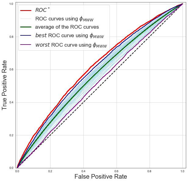
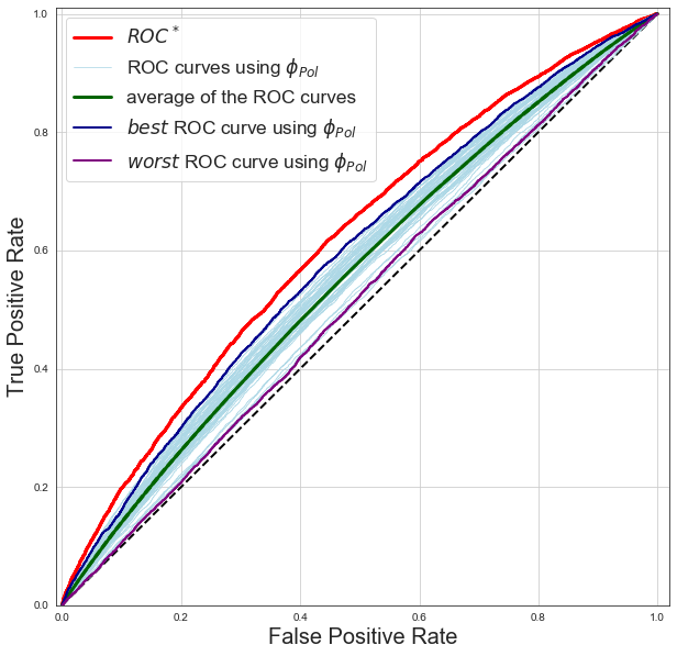
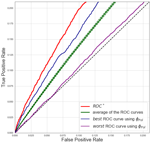
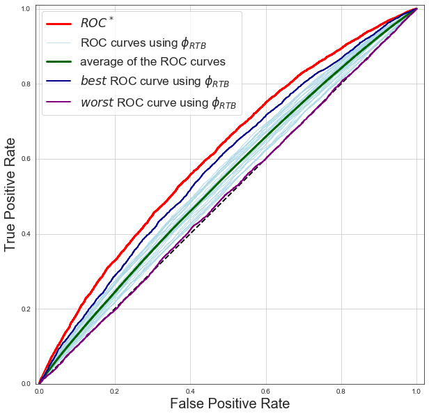
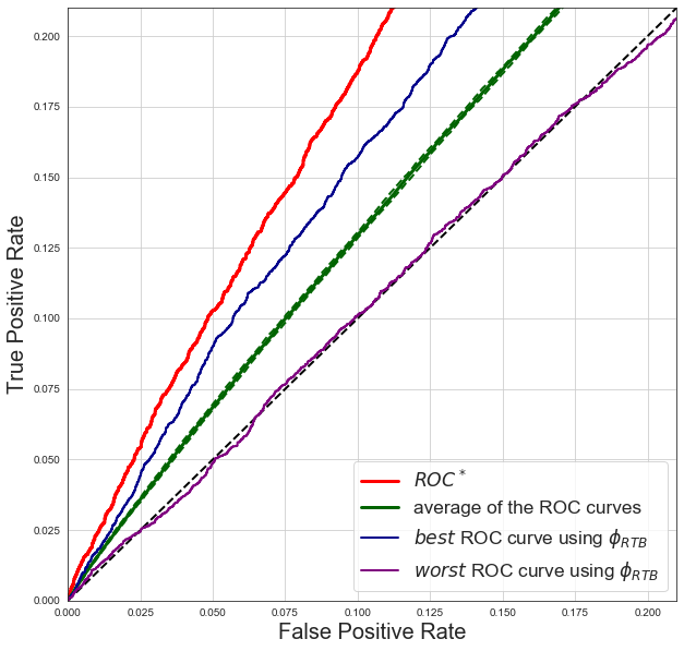
1. $\phi_{MWW}(u)=u$ 2. $\phi_{Pol}(u)=u^{3}$ 3. $\phi_{RTB}(u)=u\mathbb{I}\{u\geq 0.9\}$

Figure 10: Empirical $\rm ROC$ curves and average $\rm ROC$ curve for Loc1 ($\varepsilon=0.10$). Samples are drawn from multivariate Gaussian distributions according to section 5.2, scored with early-stopped GA algorithm’s optimal parameter for the class of scoring functions. Hyperparameters: $u_{0}=0.9$, $q=3$, $B=50$, $T=50$. Parameters for the training set: $n=m=150$; $d=15$; for the testing set: $n=m=10^{6}$; $d=15$. Figures $1,2,3$ correspond resp. to the models MMW, Pol, RTB. Light blue curves are the $B(=50)$ $\rm ROC$ curves that are averaged in green (solid line) with $+/-$ its standard deviation (dashed green lines). The dark blue and purple curves correspond to the best and worst scoring functions in the sense of minimization and maximization of the generalization error among the $B$ curves. The red curve corresponds to $\rm ROC^{*}$.

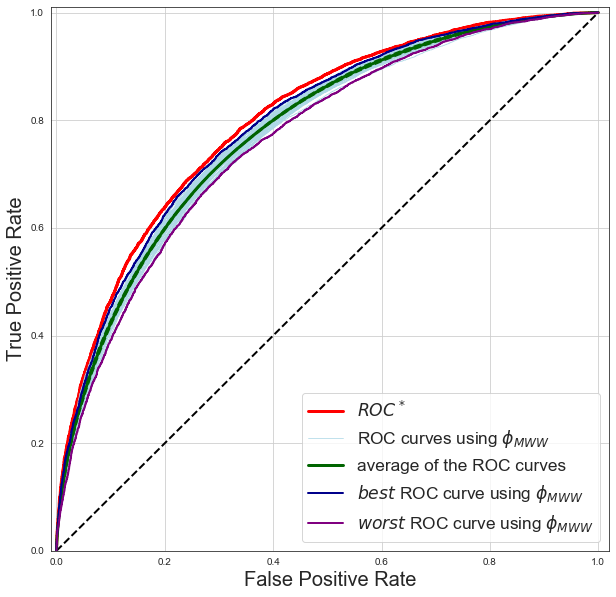
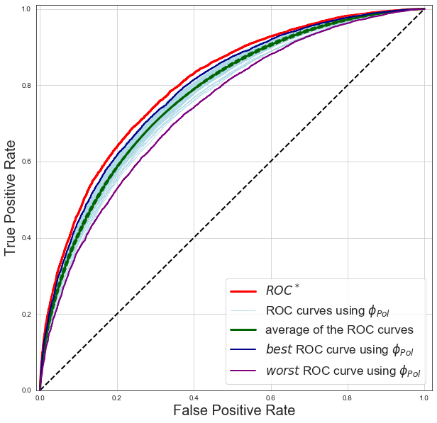
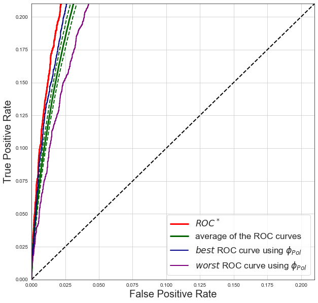
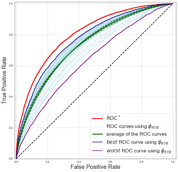
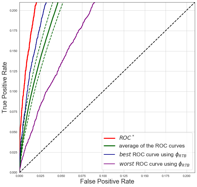
1. $\phi_{MWW}(u)=u$ 2. $\phi_{Pol}(u)=u^{3}$ 3. $\phi_{RTB}(u)=u\mathbb{I}\{u\geq 0.9\}$

Figure 11: Empirical $\rm ROC$ curves and average $\rm ROC$ curve for Loc3 ($\varepsilon=0.30$). Samples are drawn from multivariate Gaussian distributions according to section 5.2, scored with early-stopped GA algorithm’s optimal parameter for the class of scoring functions. Hyperparameters: $u_{0}=0.9$, $q=3$, $B=50$, $T=50$. Parameters for the training set: $n=m=150$; $d=15$; for the testing set: $n=m=10^{6}$; $d=15$. Figures $1,2,3$ correspond resp. to the models MMW, Pol, RTB. Light blue curves are the $B(=50)$ $\rm ROC$ curves that are averaged in green (solid line) with $+/-$ its standard deviation (dashed green lines). The dark blue and purple curves correspond to the best and worst scoring functions in the sense of minimization and maximization of the generalization error among the $B$ curves. The red curve corresponds to $\rm ROC^{*}$.

Scale model.

(Fig. 12, 13)

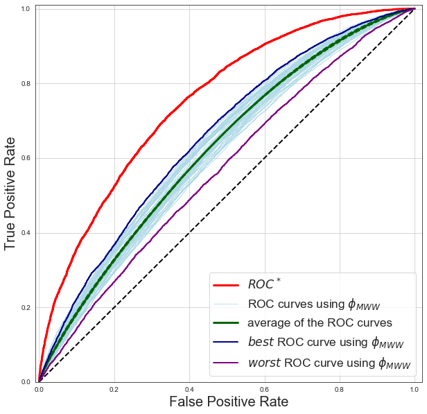
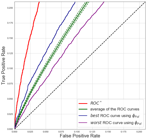
1. $\phi_{MWW}(u)=u$ 2. $\phi_{Pol}(u)=u^{3}$ 3. $\phi_{RTB}(u)=u\mathbb{I}\{u\geq 0.9\}$

Figure 12: Empirical $\rm ROC$ curves and average $\rm ROC$ curve for Scale2 ($\varepsilon=0.90$). Samples are drawn from multivariate Gaussian distributions according to section 5.2, scored with early-stopped GA algorithm’s optimal parameter for the class of scoring functions. Hyperparameters: $u_{0}=0.9$, $q=3$, $B=50$, $T=50$. Parameters for the training set: $n=m=150$; $d=15$; for the testing set: $n=m=10^{6}$; $d=15$. Figures $1,2,3$ correspond resp. to the models MMW, Pol, RTB. Light blue curves are the $B(=50)$ $\rm ROC$ curves that are averaged in green (solid line) with $+/-$ its standard deviation (dashed green lines). The dark blue and purple curves correspond to the best and worst scoring functions in the sense of minimization and maximization of the generalization error among the $B$ curves. The red curve corresponds to $\rm ROC^{*}$.

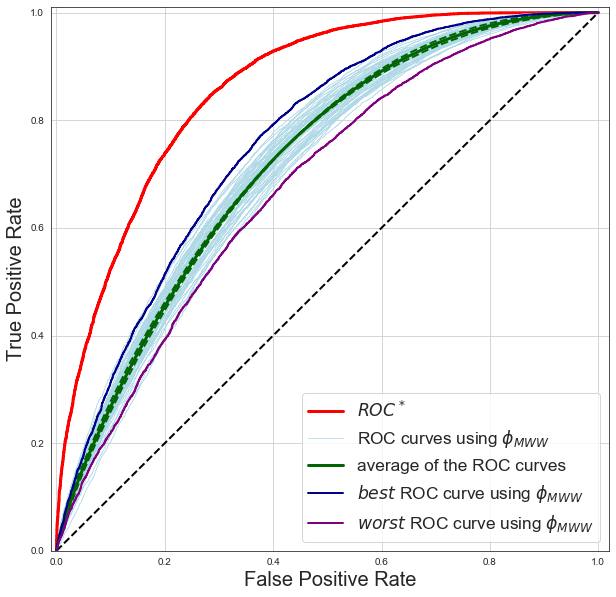
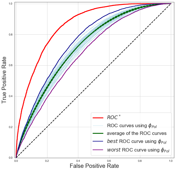
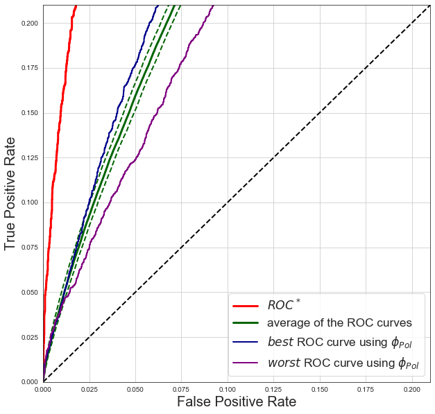
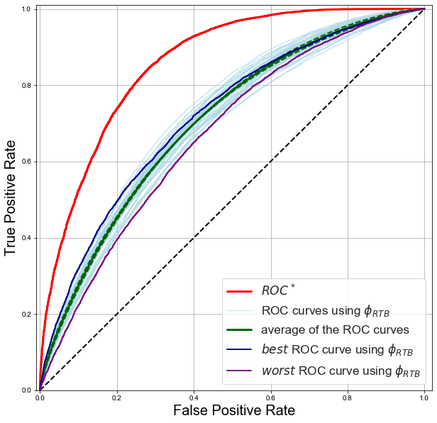
1. $\phi_{MWW}(u)=u$ 2. $\phi_{Pol}(u)=u^{3}$ 3. $\phi_{RTB}(u)=u\mathbb{I}\{u\geq 0.9\}$

Figure 13: Empirical $\rm ROC$ curves and average $\rm ROC$ curve for Scale3 ($\varepsilon=1.10$). Samples are drawn from multivariate Gaussian distributions according to section 5.2, scored with early-stopped GA algorithm’s optimal parameter for the class of scoring functions. Hyperparameters: $u_{0}=0.9$, $q=3$, $B=50$, $T=50$. Parameters for the training set: $n=m=150$; $d=15$; for the testing set: $n=m=10^{6}$; $d=15$. Figures $1,2,3$ correspond resp. to the models MMW, Pol, RTB. Light blue curves are the $B(=50)$ $\rm ROC$ curves that are averaged in green (solid line) with $+/-$ its standard deviation (dashed green lines). The dark blue and purple curves correspond to the best and worst scoring functions in the sense of minimization and maximization of the generalization error among the $B$ curves. The red curve corresponds to $\rm ROC^{*}$.

Comparison of three RTB score-generating functions for two location models.

(Fig. 14)

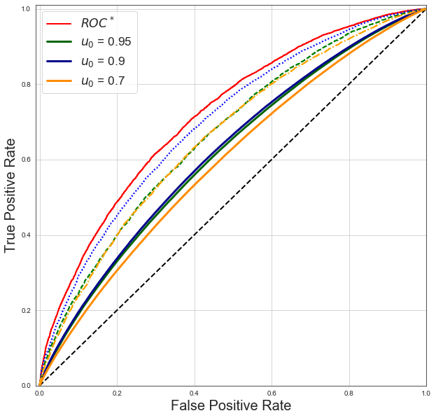
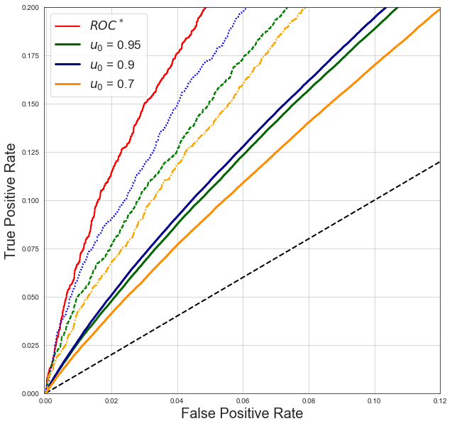
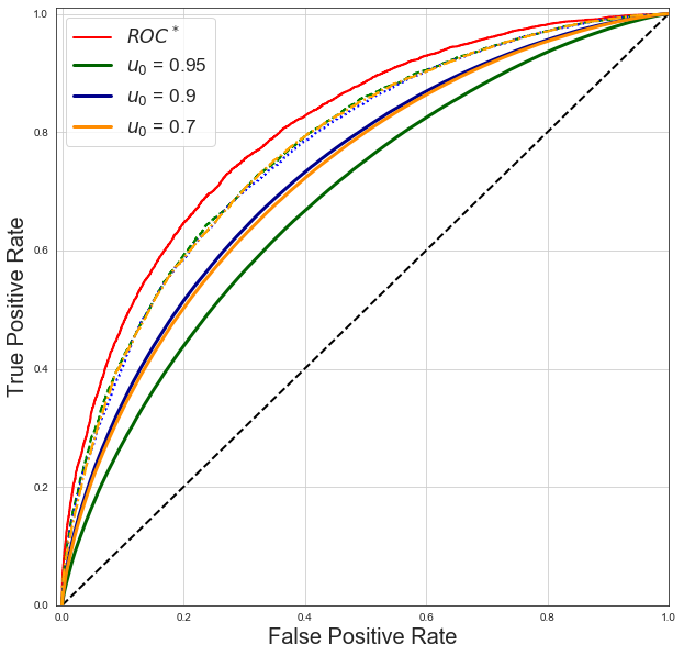
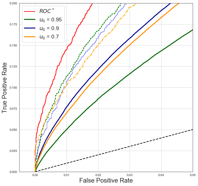
1. Loc2, $\varepsilon=0.2$ 2. Loc3, $\varepsilon=0.3$

Figure 14: Comparison of three RTB models. Average of the $\rm ROC$ curves (solid line), best $\rm ROC$ curves (dashed line) for the two location models Loc2 and Loc3. In green for $u_{0}=0.95$, blue for $u_{0}=0.90$, orange for $u_{0}=0.70$, red for $\rm ROC^{*}$. Samples are drawn from multivariate Gaussian distributions according to section 5.2, scored with early-stopped GA algorithm’s optimal parameter for the class of scoring functions and averaged after $B$ loops. Hyperparameters: $B=50$, $T=50$. Parameters for the training set: $n=m=150$; $d=15$; for the testing set: $n=m=10^{6}$; $d=15$.

Comparison of three RTB score-generating functions for the scale model.

(Fig. 15)

Figure 15: Comparison of three RTB models. Best $\rm ROC$ curves for the Scale2 model. In green for $u_{0}=0.80$, orange for $u_{0}=0.70$, green for $u_{0}=0.60$, red for $\rm ROC^{*}$. Samples are drawn from multivariate Gaussian distributions according to section 5.2, scored with early-stopped GA algorithm’s optimal parameter for the class of scoring functions and averaged after $B$ loops. Hyperparameters: $B=50$, $T=70$. Parameters for the training set: $n=m=150$; $d=15$; for the testing set: $n=m=10^{6}$; $d=15$.

References

- [1] S. Agarwal, T. Graepel, R. Herbrich, S. Har-Peled, and D. Roth. Generalization bounds for the area under the ROC curve. Journal of Machine Learning Research, 6:393–425, 2005.
- [2] S. Boucheron, O. Bousquet, and G. Lugosi. Theory of Classification: A Survey of Some Recent Advances. ESAIM: Probability and Statistics, 9:323–375, 2005.
- [3] S. Clémençon. A statistical view of clustering performance through the theory of U-processes. Journal of Multivariate Analysis, 124:42–56, 2014.
- [4] S. Clémençon, G. Lugosi, and N. Vayatis. Ranking and empirical risk minimization of U-statistics. The Annals of Statistics, 36(2):844–874, 2008.
- [5] S. Clémençon and S. Robbiano. The TreeRank Tournament Algorithm for Multipartite Ranking. Journal of Nonparametric Statistics, 27(1):107–126, 2015.
- [6] S. Clémençon, S. Robbiano, and N. Vayatis. Ranking Data with Ordinal Labels: Optimality and Pairwise Aggregation. Machine Learning, 93(1):67–104, 2013.
- [7] S. Clémençon and N. Vayatis. Ranking the best instances. Journal of Machine Learning Research, 8:2671–2699, 2007.
- [8] S. Clémençon and N. Vayatis. Empirical performance maximization based on linear rank statistics. Advances in Neural Information Processing Systems, 3559:1–15, 2009.
- [9] S. Clémençon and N. Vayatis. Tree-based ranking methods. IEEE Transactions on Information Theory, 55(9):4316–4336, 2009.
- [10] S. Clémençon and N. Vayatis. Overlaying classifiers: a practical approach to optimal scoring. Constructive Approximation, 32(3):619–648, 2010.
- [11] D. Cossock and T. Zhang. Subset ranking using regression. Proceedings of COLT 2006, 4005:605–619, 2006.
- [12] L. Devroye, L. Györfi, and G. Lugosi. A Probabilistic Theory of Pattern Recognition. Springer, 1996.
- [13] E. Giné and A. Guillou. Rates of strong uniform consistency for multivariate kernel density estimators. Annales de l’Institut Henri Poincare (B) Probability and Statistics, 38(6):907 – 921, 2002.
- [14] E. Giné, V. Koltchinskii, and J. Zinn. Weighted uniform consistency of kernel density estimators. The Annals of Probability, 32(3B):2570–2605, 2004.
- [15] E. Giné and J. Zinn. Some limit theorems for empirical processes. The Annals of Probability, 12(4):929–989, 2004.
- [16] L. Györfi, M. Köhler, A. Krzyzak, and H. Walk. A Distribution-Free Theory of Nonparametric Regression. Springer, 2002.
- [17] J. Hájek. Asymptotically most powerful rank-order tests. The Annals of Mathematical Statistics, 33(3):112–1147, 1962.
- [18] J. Hájek. Asymptotic normality of simple linear rank statistics under alternatives. The Annals of Mathematical Statistics, 39:325–346, 1968.
- [19] J. Hájek and Z. Sidák. Theory of Rank Tests. Academic Press, 1967.
- [20] W. Hoeffding. A class of statistics with asymptotically normal distribution. The Annals of Mathematical Statistics, 19:293–325, 1948.
- [21] M.C. Jones. The performance of kernel density functions in kernel distribution function estimation. Statistics and Probability Letters, 9(2):129–132, 1990.
- [22] V. Koltchinskii. Local Rademacher complexities and oracle inequalities in risk minimization. The Annals of Statistics, 34(6):2593 – 2656, 2006.
- [23] A. J. Lee. -statistics: Theory and practice. Marcel Dekker, Inc., New York, 1990.
- [24] P. Major. An estimate on the supremum of a nice class of stochastic integrals and U-statistics. Probability Theory and Related Fields, 134(3):489–537, 2006.
- [25] C. McDiarmid. On the method of bounded differences, page 148–188. London Mathematical Society Lecture Note Series. Cambridge University Press, 1989.
- [26] A.K. Menon and R.C. Williamsson. Bipartite ranking: A risk theoretic perspective. Journal of Machine Learning Research, 7:1–102, 2016.
- [27] E.A. Nadaraya. Somenew estimates for distribution functions. Theory of Probability and its Applications, 9(3):497–500, 1964.
- [28] N. Neumeyer. A central limit theorem for two-sample u-processes. Statistics and Probability Letters, 67(1):73 – 85, 2004.
- [29] D. Nolan and D. Pollard. -processes: Rates of convergence. Annals of Statistics, 15(2):780–799, 1987.
- [30] C. Rudin. Ranking with a P-Norm Push. Proceedings of COLT 2006, 4005:589–604, 2006.
- [31] R.J. Serfling. Approximation theorems of mathematical statistics. John Wiley & Sons, 1980.
- [32] M. Talagrand. Sharper Bounds for Gaussian and Empirical Processes. The Annals of Probability, 22(1):28 – 76, 1994.
- [33] E. Giné V. De la Pena. Decoupling: from dependence to independence. Springer Science and Business Media, 1999.
- [34] S. van de Geer. Empirical Processes in M-Estimation. Cambridge University Press, 2000.
- [35] A. van der Vaart. Asymptotic Statistics. Cambridge University Press, 1998.
- [36] A. van der Vaart and J. Wellner. Weak Convergence and Empirical Processes. Springer-Verlag New York, 1996.
- [37] F. Wilcoxon. Individual comparisons by ranking methods. Biometrics, 1:80–83, 1945.