Quasi-Monte Carlo Quasi-Newton for variational Bayes

Abstract

Many machine learning problems optimize an objective that must be measured with noise. The primary method is a first order stochastic gradient descent using one or more Monte Carlo (MC) samples at each step. There are settings where ill-conditioning makes second order methods such as L-BFGS more effective. We study the use of randomized quasi-Monte Carlo (RQMC) sampling for such problems. When MC sampling has a root mean squared error (RMSE) of $O(n^{-1/2})$ then RQMC has an RMSE of $o(n^{-1/2})$ that can be close to $O(n^{-3/2})$ in favorable settings. We prove that improved sampling accuracy translates directly to improved optimization. In our empirical investigations for variational Bayes, using RQMC with stochastic L-BFGS greatly speeds up the optimization, and sometimes finds a better parameter value than MC does.

1 Introduction

Many practical problems take the form

$$\min_{\theta\in\Theta\subseteq^{d}}F(\theta)\quad\text{where}\quad F(\theta)={\mathbb{E}}(f(\boldsymbol{z};\theta))$$ (1)

and $\boldsymbol{z}$ is random vector with a known distribution $p$. Classic problems of simulation-optimization (Andradóttir,, 1998) take this form and recently it has become very important in machine learning with variational Bayes (VB) (Blei et al.,, 2017) and Bayesian optimization (Frazier,, 2018) being prominent examples.

First order optimizers (Beck,, 2017) use a sequence of steps $\theta_{k+1}\leftarrow\theta_{k}-\alpha_{k}\nabla F(\theta_{k})$ for step sizes $\alpha_{k}>0$ and an operator $\nabla$ that we always take to be the gradient with respect to $\theta$. Very commonly, neither $F$ nor its gradient is available at reasonable computational cost and a Monte Carlo (MC) approximation is used instead. The update

$$\theta_{k+1}\leftarrow\theta_{k}-\alpha_{k}\nabla\hat{F}(\theta_{k})\quad\text{for}\quad\nabla\hat{F}(\theta_{k})=\frac{1}{n}\sum_{i=1}^{n}g(\boldsymbol{z}_{i};\theta)\quad\text{and}\quad g(\boldsymbol{z};\theta)=\nabla f(\boldsymbol{z};\theta)$$ (2)

for $\boldsymbol{z}_{i}\,{\buildrel\text{iid}\over{\sim}\,}p$ is a simple form of stochastic gradient descent (SGD) (Duchi,, 2018). There are many versions of SGD, notably AdaGrad (Duchi et al.,, 2011) and Adam (Kingma and Ba,, 2014) which are prominent in optimization of neural networks among other learning algorithms. Very often SGD involves sampling a mini-batch of observations. In this paper we consider SGD that samples instead some random quantities from a continuous distribution.

While a simple SGD is often very useful, there are settings where it can be improved. SGD is known to have slow convergence when the Hessian of $F$ is ill-conditioned (Bottou et al.,, 2018). When $\theta$ is not very high dimensional, the second order methods such as Newton iteration using exact or approximate Hessians can perform better. Quasi-Newton methods such as BFGS and L-BFGS (Nocedal and Wright,, 2006) that we describe in more details below can handle much higher dimensional parameters than Newton methods can while still improving upon first order methods. We note that quasi second-order methods cannot be proved to have better convergence rate than SGD. See Agarwal et al., (2012). They can however have a better implied constant.

A second difficulty with SGD is that MC sampling to estimate the gradient can be error prone or inefficient. For a survey of MC methods to estimate a gradient see Mohamed et al., (2020). Improvements based on variance reduction methods have been adopted to improve SGD. For instance Paisley et al., (2012) and Miller et al., (2017) both employ control variates in VB. Recently, randomized quasi-Monte Carlo (RQMC) methods, that we describe below, have been used in place of MC to improve upon SGD. Notable examples are Balandat et al., (2020) for Bayesian optimization and Buchholz et al., (2018) for VB. RQMC can greatly improve the accuracy with which integrals are estimated. The theory in Buchholz et al., (2018) shows how the improved integration accuracy from RQMC translates into faster optimization for SGD. The primary benefit is that RQMC can use a much smaller value of $n$. This is also seen empirically in Balandat et al., (2020) for Bayesian optimization.

Our contribution is to combine RQMC with a second order limited memory method known as L-BFGS. We show theoretically that improved integration leads to improved optimization. We show empirically for some VB examples that the optimization is improved. We find that RQMC regularly allows one to use fewer samples per iteration and in a crossed random effects example it found a better solution than we got with MC.

At step $k$ of our stochastic optimization we will use some number $n$ of sample values, $\boldsymbol{z}_{k,1},\dots,\boldsymbol{z}_{k,n}$. It is notationally convenient to group these all together into ${\mathcal{Z}}_{k}=(\boldsymbol{z}_{k,1},\dots,\boldsymbol{z}_{k,n})$. We also write

$$\bar{g}({\mathcal{Z}}_{k};\theta)=\frac{1}{n}\sum_{i=1}^{n}g(\boldsymbol{z}_{k,i};\theta)$$ (3)

for gradient estimation at step $k$.

The closest works to ours are Balandat et al., (2020) and Buchholz et al., (2018). Like Balandat et al., (2020) we incorporate RQMC into L-BFGS. Our algorithm differs in that we take fresh RQMC samples at each iteration where they had a fixed sample of size $n$ that they used in a ‘common random numbers’ approach. They prove consistency as $n\to\infty$ for both MC and RQMC sampling. Their proof for RQMC required the recent strong law of large numbers for RQMC from Owen and Rudolf, (2021). Our analysis incorporates the geometric decay of estimation error as the number $K$ of iterations increases, similar to that used by Buchholz et al., (2018) for SGD. Our error bounds include sampling variances through which RQMC brings an advantage.

An outline of this paper is as follows. Section 2 reviews the optimization methods we need. Section 3 gives basic properties of scrambled net sampling, a form of RQMC. Section 4 presents our main theoretical findings. The optimality gap after $K$ steps of stochastic quasi-Newton is $F(\theta_{K})-F(\theta^{*})$ where $\theta^{*}$ is the optimal value. Theorem 4.1 bounds the expected optimality gap by a term that decays exponentially in $K$ plus a second term that is linear in a measure of sampling variance. RQMC greatly reduces that second non-exponentially decaying term which will often dominate. A similar bound holds for tail probabilities of the optimality gap. Theorem 4.2 obtains a comparable bound for ${\mathbb{E}}(\|\theta_{K}-\theta^{*}\|^{2})$. Section 5 gives numerical examples on some VB problems. In a linear regression problem where the optimal parameters are known, we verify that RQMC converges to them at an improved rate in $n$. In logistic regression, crossed random effects and variational autoencoder examples we see the second order methods greatly outperform SGD in terms of wall clock time to improve $F$. Since the true parameters are unknown we cannot compare accuracy of MC and RQMC sampling algorithms for those examples. In some examples RQMC finds a better ELBO than MC does when both use SGD, but the BFGS algorithms find yet better ELBOs. Section 6 gives some conclusions. The proofs of our main results are in an appendix.

2 Quasi-Newton optimization

We write $\nabla^{2}F(\theta)$ for the Hessian matrix of $F(\theta)$. The classic Newton update is

$$\theta_{k+1}\leftarrow\theta_{k}-(\nabla^{2}F(\theta_{k}))^{-1}\nabla F(\theta_{k}).$$ (4)

Under ideal circumstances it converges quadratically to the optimal parameter value $\theta^{*}$. That is $\|\theta_{k+1}-\theta^{*}\|=O(\|\theta_{k}-\theta^{*}\|^{2})$. Newton’s method is unsuitable for the problems we consider here because forming $\nabla^{2}F\in^{d\times d}$ may take too much space and solving the equation in (4) can cost $O(d^{3})$ which is prohibitively expensive. The quasi-Newton methods we consider do not form explicit Hessians. We also need to consider stochastic versions of them.

2.1 BFGS and L-BFGS

The BFGS method is named after four independent discoverers: Broyden, Fletcher, Goldfarb and Shanno. See Nocedal and Wright, (2006, Chapter 6). BFGS avoids explicitly computing and inverting the Hessian of $F$. Instead it maintains at step $k$ an approximation $H_{k}$ to the inverse of $\nabla^{2}F(\theta_{k})$. After an initialization such as setting $H_{1}$ to the identity matrix, the algorithm updates $\theta$ and $H$ via

$$\theta_{k+1} \leftarrow\theta_{k}-\alpha_{k}H_{k}\nabla F(\theta_{k}),\quad\text{and}$$

$$H_{k+1} \leftarrow\Bigl{(}I-\frac{s_{k}y_{k}^{\intercal}}{s_{k}^{\intercal}y_{k}}\Bigr{)}H_{k}\Bigl{(}I-\frac{s_{k}y_{k}^{\intercal}}{s_{k}^{\intercal}y_{k}}\Bigr{)}+\frac{s_{k}s_{k}^{\intercal}}{s_{k}^{\intercal}y_{k}}$$

respectively, where

$$s_{k}=\theta_{k+1}-\theta_{k}\quad\text{and}\quad y_{k}=\nabla F(\theta_{k+1})-\nabla F(\theta_{k}).$$

The stepsize $\alpha_{k}$ is found by a line search.

Storing $H_{k}$ is a burden and the limited-memory BFGS (L-BFGS) algorithm of Nocedal, (1980) avoids forming $H_{k}$ explicitly. Instead it computes $H_{k}\nabla F(\theta_{k})$ using a recursion based on the $m$ most recent $(s_{k},y_{k})$ pairs. See Nocedal and Wright, (2006, Algorithm 7.4).

2.2 Stochastic quasi-Newton

Ordinarily in quasi-Newton algorithms the objective function remains constant through all the iterations. In stochastic quasi-Newton algorithms the sample points change at each iteration which is like having the objective function $F$ change in a random way at iteration $k$. Despite this Bottou et al., (2018) find that quasi-Newton can work well in simulation-optimization with these random changes.

We will need to use sample methods to evaluate gradients. Given ${\mathcal{Z}}=(\boldsymbol{z}_{1},\dots,\boldsymbol{z}_{n})$ the sample gradient is $\bar{g}({\mathcal{Z}};\theta)$ as given at (3). Stochastic quasi-Newton algorithms like the one we study also require randomized Hessian information.

Byrd et al., (2016) develop a stochastic L-BFGS algorithm in the mini-batch setting. Instead of adding every correction pair $(s_{k},y_{k})$ to the buffer after each iteration, their algorithm updates the buffer every $B$ steps using the averaged correction pairs. Specifically, after every $B$ iterations, for $k=t\times B$, it computes the average parameter value $\bar{\theta}_{t}=B^{-1}\sum_{j=k-B+1}^{k}\theta_{j}$ over the most recent $B$ steps. It then computes the correction pairs by $s_{t}=\bar{\theta}_{t}-\bar{\theta}_{t-1}$ and

$$y_{t}=\bar{g}(\widetilde{\mathcal{Z}}_{t};\bar{\theta}_{t})-\bar{g}(\widetilde{\mathcal{Z}}_{t};\bar{\theta}_{t-1})=\frac{1}{n}\sum_{i=1}^{n}\bigl{(}g(\bar{\theta}_{t},\tilde{\boldsymbol{z}}_{t,i})-g(\bar{\theta}_{t-1},\tilde{\boldsymbol{z}}_{t,i})\bigr{)},$$

and adds the pair $(s_{t},y_{t})$ to the buffer. Here $\widetilde{\mathcal{Z}}_{t}=(\tilde{\boldsymbol{z}}_{t,1},\dots,\tilde{\boldsymbol{z}}_{t,n})$ is a random sample of size $n=n_{h}$ Hessian update samples. The samples $\widetilde{\mathcal{Z}}_{t}$ for $t\geqslant 1$ are completely different from and independent of ${\mathcal{Z}}_{k}$ for $k\geqslant 1$ used to update gradient estimates at step $k$. This method is called SQN (stochastic quasi-Newton). As suggested by the authors, $B$ is often taken to be 10 or 20. So one can afford to use relatively large $n_{h}$ because the amortized average number of gradient evaluations per iteration is $n_{g}+2n_{h}/B$.

The objective function from Byrd et al., (2016) has the form $F(\theta)=(1/N)\sum_{i=1}^{N}f(\boldsymbol{x}_{i};\theta)$, and $\{\boldsymbol{x}_{1},\ldots,\boldsymbol{x}_{N}\}$ is a fixed training set. At each iteration, their random sample is a subset of $n\ll N$ points in the dataset, not a sample generated from some continuous distribution. However, it is straightforward to adapt their algorithm to our setting. The details are in Algorithm 1 in Section 3.

2.3 Literature review

Many authors have studied how to use L-BFGS in stochastic settings. Bollapragada et al., (2018) proposes several techniques for stochastic L-BFGS, including increasing the sample size with iterations (progressive batching), choosing the initial step length for backtracking line search so that the expected value of the objective function decreases, and computing the correction pairs using overlapping samples in consecutive steps (Berahas et al.,, 2016).

Another way to prevent noisy updates is by a lengthening strategy from Xie et al., (2020) and Shi et al., (2020). Classical BFGS would use the correction pair $(\alpha_{k}p_{k},\,g(\theta_{k}+\alpha_{k}p_{k},\boldsymbol{z})-g(\theta_{k},\boldsymbol{z}))$, where $p_{k}=-H_{k}g(\theta_{k},\boldsymbol{z})$ is the update direction, and $\boldsymbol{z}$ encodes the randomness in estimating the gradients. Because the correction pairs may be dominated by noise, Xie et al., (2020) suggested the lengthening correction pairs

$$(s_{k},\,y_{k})=(\beta_{k}p_{k},\,g(\theta_{k}+\beta_{k}p_{k})-g(\theta_{k})),\quad\text{where }\beta_{k}\geqslant\alpha_{k}.$$

Shi et al., (2020) propose to choose $\alpha_{k}$ by the Armijo-Wolfe condition, while choosing $\beta_{k}$ large enough so that $[g(\theta_{k}+\beta_{k}p_{k})-g(\theta_{k})]^{\intercal}p_{k}/\|p_{k}\|$ is sufficiently large.

Gower et al., (2016) utilizes sketching strategies to update the inverse Hessian approximations by compressed Hessians. Moritz et al., (2016) combines the stochastic quasi-Newton algorithm in Byrd et al., (2016) and stochastic variance reduced gradients (SVRG) (Johnson and Zhang,, 2013) by occasionally computing the gradient using a full batch.

Balandat et al., (2020) also applied RQMC with L-BFGS in Bayesian optimization. At each step of Bayesian optimization, one needs to maximize the acquisition function of the form $\alpha(\theta):=\mathbb{E}\left[\ell(g(\theta))\right]$, where $g$ is a Gaussian process and $\ell$ is a loss function. They use the sample average approximation $\hat{\alpha}(\theta):=(1/n)\sum_{i=1}^{n}\ell(\xi_{i}(\theta))$, where $\xi_{i}(\theta)\sim g(\theta)$. They prove that the maximizer of $\hat{\alpha}$ converges to that of $\alpha$ when $n\rightarrow\infty$ for both MC and RQMC sampling under certain conditions. The RQMC result relies on the recent discovery of the strong law of large numbers for RQMC (Owen and Rudolf,, 2021).

3 Scrambled net sampling

Scrambled nets are a form of RQMC sampling. We begin by briefly describing plain quasi-Monte Carlo (QMC) sampling. QMC is most easily described for computing expectations of $f(\boldsymbol{u})$ for $\boldsymbol{u}\sim\mathbf{U}[0,1]^{s}$. In our present context $f(\cdot)$ will be a component of $g(\cdot;\theta)$ and not the same as the $f$ in equation (1). In practice we must ordinarily transform the random variables $\boldsymbol{u}$ to some other distribution such as a Gaussian via $\boldsymbol{x}=\psi(\boldsymbol{u})$. We suppose that $\psi(\boldsymbol{u})\sim p$ for some transformation $\psi(\cdot)$. The text by Devroye, (1986) has many examples of such transformations. Here we subsume any such transformation $\psi(\cdot)$ into the definition of $f$.

In QMC sampling, we estimate $\mu=\int_{[0,1]^{s}}f(\boldsymbol{u})\mathrm{\,d}\boldsymbol{u}$ by $\hat{\mu}=(1/n)\sum_{i=1}^{n}f(\boldsymbol{u}_{i})$, just like in MC sampling except that distinct points $\boldsymbol{u}_{i}$ are chosen so that the discrete uniform distribution $\mathbf{U}\{\boldsymbol{u}_{1},\dots,\boldsymbol{u}_{n}\}$ is made very close to the continuous $\mathbf{U}[0,1]^{s}$ distribution. The difference between these two distributions can be quantified in many ways, called discrepancies (Chen et al.,, 2014). For a comprehensive treatment of QMC see Dick and Pillichshammer, (2010) or Niederreiter, (1992) or Dick et al., (2013).

When $f$ is of bounded variation in the sense of Hardy and Krause (BVHK) (see Owen, (2005)) then QMC attains the asymptotic error rate $|\hat{\mu}-\mu|=O(n^{-1}\log(n)^{s-1})=O(n^{-1+\epsilon})$ for any $\epsilon>0$. QMC is deterministic and to get practical error estimates RQMC methods were introduced. In RQMC, each individual $\boldsymbol{u}_{i}\sim\mathbf{U}[0,1]^{d}$ while collectively $\boldsymbol{u}_{1},\dots,\boldsymbol{u}_{n}$ still retain the low discrepancy property. Uniformity of $\boldsymbol{u}_{i}$ makes RQMC unbiased: ${\mathbb{E}}(\hat{\mu})=\mu$. Then if $f\in\mathrm{BVHK}$ we get an RMSE of $O(n^{-1+\epsilon})$. The whole RQMC process can then be replicated independently to quantify uncertainty. See Cranley and Patterson, (1976) and Owen, (1995) for methods and a survey in L’Ecuyer and Lemieux, (2002).

Scrambled net sampling (Owen,, 1995) is a form of RQMC that operates by randomly permuting the bits (more generally digits) of QMC methods called digital nets. The best known are those of Sobol’, (1969) and Faure, (1982). In addition to error estimation, scrambled nets give the user some control over the powers of $\log(n)$ in the QMC rate and also extend the domain of QMC from Riemann integrable functions of which BVHK is a subset to much more general functions including some with integrable singularities. For any integrand $f\in L^{2}[0,1]^{s}$, MC has RMSE $O(n^{-1/2})$ while scrambled nets have RMSE $o(n^{-1/2})$ without requiring $f\in\mathrm{BVHK}$ or even that $f$ is Riemann integrable (Owen, 1997a, ). For fixed $n$, each construction of scrambled nets has a ‘gain constant’ $\Gamma<\infty$ so that the RMSE is below $\sqrt{\Gamma}n^{-1/2}$ for any $f\in L^{2}[0,1]^{s}$. This effectively counters the powers of $\log(n)$. For smooth enough $f$, an error cancellation phenomenon for scrambled nets yields an RMSE of $O(n^{-3/2}\log(n)^{(s-1)/2})=O(n^{-3/2+\epsilon})$ (Owen, 1997b, ; Yue and Mao,, 1999; Owen,, 2008). The logarithmic powers here cannot ‘set in’ until they are small enough to obey the $\Gamma^{1/2}n^{-1/2}$ upper bound. Some forms of scrambled net sampling satisfy a central limit theorem (Loh,, 2003; Basu and Mukherjee,, 2017).

Very recently, a strong law of large numbers

$$\Pr\Bigl{(}\lim_{n\to\infty}\hat{\mu}_{n}=\mu\Bigr{)}=1$$

has been proved for scrambled net sampling assuming only that $f\in L^{1+\delta}[0,1]^{s}$ for some $\delta>0$ (Owen and Rudolf,, 2021). The motivation for this result was that Balandat et al., (2020) needed a strong law of large numbers to prove consistency for their use for scrambled nets in Bayesian optimization.

Figure 1 graphically compares MC, QMC and RQMC points for $s=2$. The underlying QMC method is a Sobol’ sequence using ‘direction numbers’ from Joe and Kuo, (2008). We can see that MC points leave voids and create clumps. The QMC points are spread out more equally and show a strong diagonal structure. The RQMC points satisfy the same discrepancy bounds as the QMC points do but have broken up some of the structure.

Figure 1: Each panel shows $512$ points in $[0,1]^{2}$. From left to right they are plain MC, Sobol’ points and scrambled Sobol’ points. From Owen and Rudolf, (2021): Copyright © 2021 Society for Industrial and Applied Mathematics. Reprinted with permission. All rights reserved.

In favorable settings the empirical behaviour of QMC and RQMC for realistic $n$ can be as good as their asymptotic rates. In less favorable settings RQMC can be like MC with some reduced variance. The favorable integrands are those where $f$ is nearly additive or at least dominated by sums of only a few of their inputs at a time. See Caflisch et al., (1997) for a definition of functions of ‘low effective dimension’ and Dick et al., (2013) for a survey of work on reproducing kernel Hilbert spaces of favorable integrands.

We propose to combine the stochastic quasi-Newton method with RQMC samples to create a randomized quasi-stochastic quasi-Newton (RQSQN) algorithm. At the $k$’th iteration, we draw an independently scrambled refreshing sample ${\mathcal{Z}}_{k}=(\boldsymbol{z}_{k,1},\dots,\boldsymbol{z}_{k,n_{g}})$ of size $n=n_{g}$ via RQMC to compute the gradient estimator $\bar{g}({\mathcal{Z}}_{k};\theta_{k})$. Then we find the descent direction $H_{k}\bar{g}({\mathcal{Z}}_{k};\theta_{k})$ using an L-BFGS two-loop recursion. Then we update the solution by

$$\theta_{k+1}\leftarrow\theta_{k}-\alpha_{k}H_{k}\bar{g}({\mathcal{Z}}_{k};\theta_{k}).$$

Here $\alpha_{k}$ may be found by line search with the Wolfe condition when using L-BFGS. See Chapter 3.1 in Nocedal and Wright, (2006).

Algorithm 1 shows pseudo-code for an RQMC version of SQN based on L-BFGS. It resembles the SQN algorithm in Byrd et al., (2016), except that the random samples are drawn by using RQMC instead of being sampled without replacement from a finite data set. Note that we don’t compute the Hessian directly. We either compute the Hessian-vector product $\nabla^{2}f({\mathcal{Z}}_{t};\bar{\theta}_{t})s_{t}$ or use gradient differences $\nabla f(\bar{\theta}_{t})-\nabla f(\bar{\theta}_{t-1})$.

Input : Initialization $\theta_{1}$, buffer size $m$, Hessian update interval $B$, sample sizes $n_{g}$ and $n_{h}$ for estimating gradient and updating buffer

Output : Solution $\theta$

$t\leftarrow-1$;

for $k=1,2,\ldots$ do

       Take an RQMC sample $\boldsymbol{z}_{k,1},\ldots,\boldsymbol{z}_{k,n_{g}}\sim p$;

       Calculate the gradient estimator $g_{k}\leftarrow\bar{g}({\mathcal{Z}}_{k};\theta_{k})=\frac{1}{n_{g}}\sum_{i=1}^{n_{g}}g(\boldsymbol{z}_{k,i};\theta_{k})$;

       if $t<1$ then

             $\theta_{k+1}\leftarrow\theta_{k}-\alpha_{k}g_{k}$;

            

      else

             Find $H_{t}g_{k}$ by the two-loop recursion with memory size $m$;

             Find $\alpha_{k}$ by line search;

             Update $\theta_{k+1}\leftarrow\theta_{k}-\alpha_{k}H_{t}g_{k}$;

            

      

      if $\mod(k,B)=0$ then

             $t\leftarrow t+1$;

             $\bar{\theta}_{t}\leftarrow B^{-1}\sum_{j=k-B+1}^{k}\theta_{j}$;

             if $t>0$ then

                  

                  Take an RQMC sample $\tilde{\boldsymbol{z}}_{t,1},\ldots,\tilde{\boldsymbol{z}}_{t,n_{h}}\sim p$;

                   Add $s_{t}=(\bar{\theta}_{t}-\bar{\theta}_{t-1})$, $y_{t}=\bar{g}(\widetilde{\mathcal{Z}}_{t};\bar{\theta}_{t})=\frac{1}{n_{h}}\sum_{i=1}^{n_{h}}\nabla^{2}f(\tilde{\boldsymbol{z}}_{t,i};\bar{\theta}_{t})s_{t}$ to the buffer;

                  

            

      

Algorithm 1 RQMC-SQN

4 Theoretical guarantees

In this section, we study the convergence rate of a general quasi-Newton iteration based on $n$ sample points $\boldsymbol{z}_{k1},\dots,\boldsymbol{z}_{kn}\sim p$ at stage $k$. The algorithm iterates as follows

$$\theta_{k+1} \leftarrow\theta_{k}-\alpha_{k}H_{k}\nabla\bar{f}({\mathcal{Z}}_{k};\theta_{k}),\quad\text{where}$$ (5)

$$\nabla\bar{f}({\mathcal{Z}}_{k};\theta_{k}) =\frac{1}{n}\sum_{i=1}^{n}\nabla f(\boldsymbol{z}_{ki};\theta_{k})=\bar{g}({\mathcal{Z}}_{k};\theta_{k}).$$

Here $H_{k}$ is an approximate inverse Hessian. We let $F(\theta)={\mathbb{E}}(f(\boldsymbol{z}_{ki};\theta))$. We assume that the gradient estimator $g({\mathcal{Z}}_{k};\theta_{k})$ is unbiased conditionally on $\theta_{k}$, i.e., ${\mathbb{E}}(g({\mathcal{Z}}_{k};\theta_{k})\mid\theta_{k})=\nabla F(\theta_{k})$. The $\theta_{k}$ are random because they depend on ${\mathcal{Z}}_{k^{\prime}}$ for $k^{\prime}<k$.

The Hessian estimates $H_{k}$ for $k>1$ are also random because they depend directly on some additional inputs $\tilde{\mathcal{Z}}_{t}$ for those Hessian update epochs $t$ which occur prior to step $k$. They also depend on ${\mathcal{Z}}_{k^{\prime}}$ for $k^{\prime}<k$ because those random variables affect $\theta_{k^{\prime}}$. In our algorithms $H_{k}$ is independent of $\theta_{k}$. For RQMC this involves fresh rerandomizations of the underlying QMC points at step $k$. The alternative of ‘going deeper’ into a given RQMC sequence using points $(k-1)n+1$ through $kn$ would not satisfy independence. While it might possibly perform better it is harder to analyze and we saw little difference empirically in doing that. Our theory requires regularity of the problem as follows.

Assumption 1

We impose these three conditions:

1. Strong convexity. For some $c>0$,

   $$F(\theta^{\prime})\geqslant F(\theta)+\nabla F(\theta)^{\intercal}(\theta^{\prime}-\theta)+\frac{c}{2}\|\theta^{\prime}-\theta\|_{2}^{2}\quad\text{for all}\quad\theta,\theta^{\prime}\in\Theta.$$

2. Lipschitz continuous objective gradients. For some $L<\infty$,

   $$\|\nabla F(\theta)-\nabla F(\theta^{\prime})\|\leqslant L\|\theta-\theta^{\prime}\|\quad\text{for all}\quad\theta,\theta^{\prime}\in\Theta.$$

3. Bounded variance of the gradient estimator. For some $M<\infty$,

   $${\mathrm{tr}}\bigl{(}{\mathrm{Var}}(\bar{g}({\mathcal{Z}}_{k};\theta_{k})\!\mid\!\theta_{k})\bigr{)}\leqslant M\quad\text{for all}\quad k\geqslant 1.$$

These are standard assumptions in the study of SGD. For example, see Assumptions 4.1 and 4.5 of Bottou et al., (2018). Strong convexity implies that there exists a unique minimizer $\theta^{*}$ to estimate. We write $F^{*}=F(\theta^{*})$, for the best possible value of $F$. We must have some smoothness and Lipshitz continuity is a mild assumption. The quantity $M$ will prove to be important below. We can get a better $M$ from RQMC than from MC. The other way to reduce $M$ is to increase $n$. When RQMC has an advantage it is because it gets a smaller $M$ for the same $n$, or to put it another way, it can get comparable $M$ with smaller $n$.

For two symmetric matrices $A$ and $B$, $A\preccurlyeq B$ means that $B-A$ is positive semi-definite. We denote the spectral norm of $A$ by $\|A\|$.

Theorem 4.1 (Convergence of optimality gap)

Suppose that our simulation-optimization problem satisfies the regularity conditions in Assumption 1. Assume that we run updates as in equation (5) where the approximate inverse Hessian matrices $H_{k}$ satisfy $h_{1}I\preccurlyeq H_{k}\preccurlyeq h_{2}I$ for some $0<h_{1}\leqslant h_{2}$ and all $k\geqslant 1$. Next, assume constant step sizes $\alpha_{k}=\alpha$ with $0<\alpha\leqslant h_{1}/(Lh_{2}^{2})$. Then for every $K\geqslant 1$

$${\mathbb{E}}(F(\theta_{K})-F^{*}) \leqslant(1-\alpha ch_{1})^{K}(F(\theta_{0})-F^{*})+\frac{\alpha Lh_{2}^{2}}{2ch_{1}}M.$$ (6)

Furthermore, if $\|g(\theta,\boldsymbol{z})\|\leqslant C$ for some constant $C$ for all $\theta$ and $\boldsymbol{z}$, then for any $\varepsilon>0$

$$F(\theta_{K})-F^{*} \leqslant(1-\alpha ch_{1})^{K}(F(\theta_{0})-F^{*})+\frac{\alpha Lh_{2}^{2}}{2ch_{1}}M+C^{2}\sqrt{\frac{2\alpha}{ch_{1}}}\bigl{(}h_{2}-L\alpha h_{1}^{2}+{h_{1}}{}\bigr{)}\varepsilon$$ (7)

holds with probability at least $1-e^{-\varepsilon^{2}}$.

Proof  See Section A.1 in the Appendix.  

Remark 4.1

As $K\rightarrow\infty$ the expected optimality gap is no larger than $[(\alpha Lh_{2}^{2})/(2ch_{1})]\times M$. The variance bound $M=M(n)$ (for $n$ points $\boldsymbol{z}_{k,i}$) depends on the sampling method we choose. From the results in Section 3, scrambled nets can reduce $M$ from $O(1/n)$ for MC to $o(1/n)$ attaining $O(n^{-2+\epsilon})$ or even $O(n^{-3+\epsilon})$ in favorable cases. When $M<\infty$ for MC then $M\leqslant\Gamma M$ for scrambled net RQMC, which limits the harm if any that could come from RQMC.

Remark 4.2

By Lemma 3.1 of Byrd et al., (2016), the L-BFGS iteration satisfies $h_{1}I\preccurlyeq H_{k}\preccurlyeq h_{2}I$ under weaker conditions than we have in Theorem 4.1. We can replace the bound $\|g(\boldsymbol{z};\theta)\|\leqslant C$ by ${\mathbb{E}}(\|g(\boldsymbol{z};\theta)\|^{2})\leqslant C^{2}<\infty$.

The following theorem states the convergence rate of $\|\theta_{k}-\theta^{*}\|$.

Theorem 4.2 (Convergence of variables)

Under the conditions of Theorem 4.1, suppose that

$$\frac{c}{L}>\frac{h_{2}-h_{1}}{h_{2}+h_{1}}\quad\text{and}\quad 0<\alpha_{k}<\frac{(h_{1}+h_{2})c-(h_{2}-h_{1})L}{2L^{2}h_{2}^{2}}.$$

Then for every $K\geqslant 1$,

$${\mathbb{E}}(\|\theta_{K}-\theta^{*}\|^{2})\leqslant\bigl{(}1-\alpha^{2}h_{2}^{2}L^{2}\bigr{)}^{K}\|\theta_{0}-\theta^{*}\|^{2}+M/L^{2}.$$

Proof  See Section A.2 in the Appendix.  

Remark 4.3

When $K\rightarrow\infty$, the limiting expected squared error is bounded by $\alpha^{2}h_{2}^{2}M$. Once again the potential gain from RQMC is in reducing $M$ compared to MC or getting a good $M$ with smaller $n$.

5 Variational Bayes

In this section we investigate quasi-Newton quasi-Monte Carlo optimization for some VB problems. Variational Bayes begins with a posterior distribution $p(\boldsymbol{z}\!\mid\!\boldsymbol{x})$ that is too inconvenient to work with. This usually means that we cannot readily sample $\boldsymbol{z}$. We turn instead to a distribution $q_{\theta}$ for $\theta\in\Theta$ from which we can easily sample $\boldsymbol{z}\sim q_{\theta}$. We now want to make a good choice of $\theta$ and in VB the optimal value $\theta^{*}$ is taken to be the minimizer of the KL divergence between distributions:

$$\theta^{*}=\operatorname*{argmin}_{\theta\in\Theta}\,\mathcal{D}_{\mathrm{KL}}(q_{\theta}(\boldsymbol{z})\,\|\,p(\boldsymbol{z}\!\mid\!\boldsymbol{x})).$$

In this section we are using the symbol $p(\cdot)$ as a generic probability distribution. It is the distribution of whatever random variable’s symbol is inside the parentheses and not necessarily the same $p$ from the introduction. We use ${\mathbb{E}}_{\theta}(\cdot)$ to denote expectation with respect to $\boldsymbol{z}\sim q_{\theta}$.

We suppose that $\boldsymbol{z}$ has a prior distribution $p(\boldsymbol{z})$. Then Bayes rule gives

$$\mathcal{D}_{\mathrm{KL}}(q_{\theta}(\boldsymbol{z})\,\|\,p(\boldsymbol{z}\!\mid\!\boldsymbol{x})) ={\mathbb{E}}_{\theta}\bigl{(}{\log q_{\theta}(\boldsymbol{z})-\log p(\boldsymbol{z}\!\mid\!\boldsymbol{x})}\bigr{)}$$

$$={\mathbb{E}}_{\theta}\Bigl{(}{\log q_{\theta}(\boldsymbol{z})-\log\frac{p(\boldsymbol{x}\!\mid\!\boldsymbol{z})p(\boldsymbol{z})}{p(\boldsymbol{x})}}\Bigr{)}$$

$$=\mathcal{D}_{\mathrm{KL}}(q_{\theta}(\boldsymbol{z})\,\|\,p(\boldsymbol{z}))-{\mathbb{E}}_{\theta}(p(\boldsymbol{x}\!\mid\!\boldsymbol{z}))+\log p(\boldsymbol{x}).$$

The last term does not depend on $\theta$ and so we may minimize $\mathcal{D}_{\mathrm{KL}}(\cdot\,\|\,\cdot)$ by maximizing

$${\mathcal{L}}(\theta)={\mathbb{E}}_{\theta}({\log p(\boldsymbol{x}\!\mid\!\boldsymbol{z})})-\mathcal{D}_{\mathrm{KL}}(q_{\theta}(\boldsymbol{z})\,\|\,p(\boldsymbol{z})).$$

This ${\mathcal{L}}(\cdot)$ is known as the evidence lower bound (ELBO). The first term ${\mathbb{E}}_{\theta}({\log p(\boldsymbol{x}\!\mid\!\boldsymbol{z})})$ expresses a preference for $\theta$ having a large value of the likelihood of the observed data $\boldsymbol{x}$ given the latent data $\boldsymbol{z}$. The second term $-\mathcal{D}_{\mathrm{KL}}(q_{\theta}(\boldsymbol{z}\,\|\,p(\boldsymbol{z}))$ can be regarded as a regularization, penalizing parameter values for which $q_{\theta}(\boldsymbol{z})$ is too far from the prior distribution $p(\boldsymbol{z})$.

To optimize ${\mathcal{L}}(\theta)$ we need $\nabla{\mathcal{L}}(\theta)$. It is usual to choose a family $q_{\theta}$ for which $\mathcal{D}_{\mathrm{KL}}(\cdot\,\|\,\cdot)$ and its gradient are analytically tractable. We still need to estimate the gradient of the first term, i.e.,

$$\nabla\,{\mathbb{E}}_{\theta}({\log p(\boldsymbol{x}\!\mid\!\boldsymbol{z})}).$$

One method is to use the score function $\nabla\log p_{\theta}(z)$ and Fisher’s identity

$$\nabla{\mathbb{E}}_{\theta}({f(\boldsymbol{z})})={\mathbb{E}}_{\theta}({f(\boldsymbol{z})\nabla\log p_{\theta}(\boldsymbol{z})})$$

with $f(\cdot)=\log(p(\boldsymbol{x}\!\mid\!\cdot))$. Unfortunately an MC strategy based on this approach can suffer from large variance.

The most commonly used method is to write the parameter $\theta$ as a function of some underlying common random variables. This is known as the reparameterization trick (Kingma and Welling,, 2014). Suppose that there is a base distribution $p_{0}$ and a transformation $T(\cdot;\theta)$, such that if $\boldsymbol{z}\sim p_{0}$, then $T(\boldsymbol{z};\theta)\sim q_{\theta}$. Then

$$\nabla{\mathbb{E}}_{\theta}({f(\theta)})={\mathbb{E}}_{p_{0}}(\nabla f(T(\boldsymbol{z};\theta))).$$

It is often easy to sample from the base distribution $p_{0}$, and thus to approximate the expectation by MC or RQMC samples. This is the method we use in our examples.

5.1 Bayesian linear regression

We start with a toy example where we can find $\theta^{*}$ analytically. This will let us study $\|\theta_{k}-\theta^{*}\|$ empirically. We consider the hierarchical linear model

$$\boldsymbol{y}\!\mid\!\beta\sim\mathcal{N}(X\beta,\gamma^{2}I_{N})\quad\text{for}\quad\beta\sim\mathcal{N}(0,I_{d})$$

where $X\in^{N\times d}$ is a given matrix of full rank $d\leqslant N$ and $\gamma^{2}\in(0,\infty)$ is a known error variance. Here $N$ is the number of data points in our simulation and not the number $n$ of MC or RQMC gradient evaluations. The entries in $X$ are IID $\mathcal{N}(0,1)$ random variables and we used $\gamma=0.5$.

Translating this problem into the VB setup, we make our latent variable $\boldsymbol{z}$ the unknown parameter vector $(\beta_{1},\dots,\beta_{d})$, and we choose a very convenient variational distribution $q_{\theta}$ with $\beta_{j}\stackrel{{\scriptstyle\mathrm{ind}}}{{\sim}}\mathcal{N}(\mu_{j},\sigma_{j}^{2})$ for $j=1,\ldots,d$. Now $\theta=(\mu_{1},\dots,\mu_{d},\sigma_{1},\dots,\sigma_{d})$, and $\boldsymbol{y}$ plays the role of the observations $\boldsymbol{x}$. We also write $\mu=(\mu_{1},\dots,\mu_{d})$ and $\sigma=(\sigma_{1},\dots,\sigma_{d})$ for the parts of $\theta$.

The ELBO has the expression

$${\mathcal{L}}(\theta) ={\mathbb{E}}_{\theta}({\log p(\boldsymbol{y}\!\mid\!\beta)})-\mathcal{D}_{\mathrm{KL}}(q_{\theta}(\beta)\,\|\,p(\beta\!\mid\!\boldsymbol{y}))$$

$$={\mathbb{E}}_{\theta}({\log p(\boldsymbol{y}\!\mid\!\beta)})-\sum_{j=1}^{d}\Bigl{(}\frac{\sigma_{j}^{2}+\mu_{j}^{2}-1}{2}-\log\sigma_{j}\Bigr{)},$$

where $\log p(\boldsymbol{y}\!\mid\!\beta)=-(p/2)\log(2\pi\gamma^{2})-\|\boldsymbol{y}-X\beta\|_{2}^{2}/(2\gamma^{2})$. In this example, the ELBO has a closed form and the optimal variational parameters are given by

$$\mu^{*} =\Bigl{(}\frac{X^{\intercal}X}{\gamma^{2}}+I_{d}\Bigr{)}^{-1}\frac{X^{\intercal}\boldsymbol{y}}{\gamma^{2}}\quad\text{and}\quad\sigma^{*}_{j}=\Bigl{(}1+\frac{\|X_{\text{\tiny$\bullet$}j}\|^{2}}{\gamma^{2}}\Bigr{)}^{-1/2},$$

where $X_{\text{\tiny$\bullet$}j}\in^{N}$ is the $j$’th column of $X$.

In this setting the Hessian is simply $-X^{\intercal}X/\gamma^{2}$ and so stochastic quasi-Newton gradient estimates are not needed. We can however compare the effectiveness of MC and RQMC in SGD. We estimate the gradient by MC or RQMC samples and use SGD via AdaGrad (Duchi et al.,, 2011) to maximize the ELBO.

Our computations used one example data set with $N=300$ data points, $d=100$ variables and $K=1000$ iterations. At each iteration, we draw a new sample of sample size $n$ of the $d$-dimensional Gaussian used to sample $\beta$. The sample size $n$ is fixed in each run, but we vary it between over the range $8\leqslant n\leqslant 8192$ through powers of $2$ in order to explore how quickly MC and RQMC converge.

For RQMC, we use the scrambled Sobol’ points implemented in PyTorch (Balandat et al.,, 2020) using the inverse Gaussian CDF $\psi(\cdot)=\Phi^{-1}(\cdot)$ to translate uniform random variables into standard Gaussians that are then multiplied by $\sigma_{j}$ and shifted by $\mu_{j}$ to get the random $\beta_{j}$ that we need. We compute the log errors $\log_{2}\|{\mathcal{L}}_{k}-{\mathcal{L}}^{*}\|$ and $\log_{2}\|\theta_{k}-\theta^{*}\|$ and average these over the last 50 iterations. The learning rate in AdaGrad was taken to be $1$.

The results are shown in Figure 2. We see there that RQMC achieves a higher accuracy than plain MC. This happens because RQMC estimates the gradient with lower variance. In this simple setting the rate of convergence is improved. Balandat et al., (2020) report similar rate improvements in Bayesian optimization.

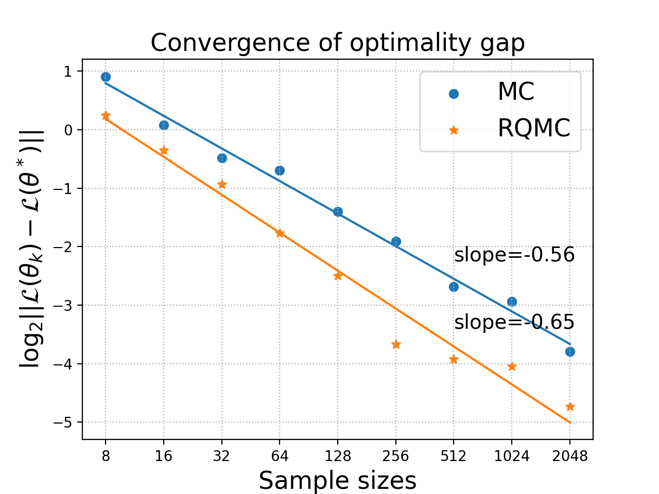
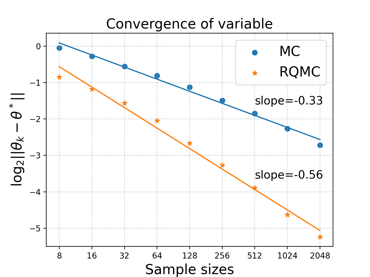
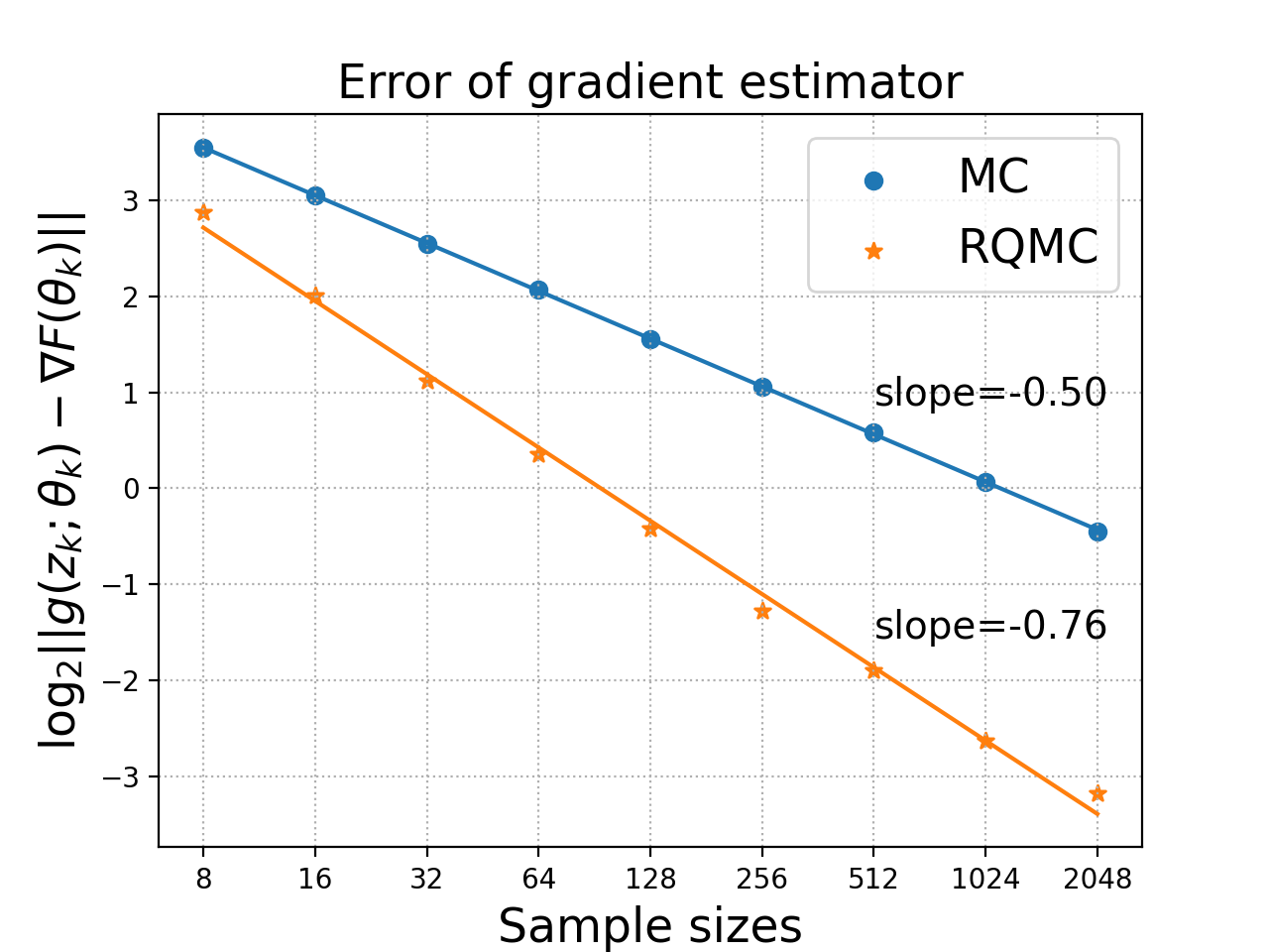
Figure 2: The left panel has the average of $\log_{2}|{\mathcal{L}}(\theta_{k})-{\mathcal{L}}(\theta^{*})|$ over the last $50$ values of $k$ versus $n$. The middle panel has that average of $\log_{2}\|\theta_{k}-\theta^{*}\|$. The right panel has the average of $\log_{2}\|g(\boldsymbol{z}_{k};\theta_{k})-\nabla F(\theta_{k})\|$ versus $n$ where $\hat{g}(\hat{\theta}_{k})=(1/n)\sum_{i=1}^{n}g(\boldsymbol{z}_{k,i};\theta_{k})$. The straight lines are least squares fits with their slopes written above them.

5.2 Bayesian logistic regression

Next we consider another simple example, though it is one with no closed form expression for $\theta^{*}$. We use it to compare first and second order methods. The Bayesian logistic regression model is defined by

$$\Pr(y_{i}=\pm 1\!\mid\!\boldsymbol{x}_{i},\beta) =\frac{1}{1+\exp(\mp\boldsymbol{x}_{i}^{\intercal}\beta)},\quad i=1,\ldots,N\quad\text{where}\quad\beta\sim\mathcal{N}(0,I_{d}).$$

As before, $\beta$ is the unknown $\boldsymbol{z}$, and $p_{\theta}$ has $\beta_{j}\stackrel{{\scriptstyle\mathrm{ind}}}{{\sim}}\mathcal{N}(\mu_{j},\sigma_{j}^{2})$, for $\theta=(\mu_{1},\dots,\mu_{d},\sigma_{1},\dots,\sigma_{d})$. The ELBO has the form

$${\mathcal{L}}_{\theta} ={\mathbb{E}}_{\theta}\biggl{(}\,{\sum_{i=1}^{N}\log S(y_{i}\boldsymbol{x}_{i}^{\intercal}\beta)}\biggr{)}-\sum_{j=1}^{d}\Bigl{(}\frac{\sigma_{j}^{2}+\mu_{j}^{2}-1}{2}-\log\sigma_{j}\Bigr{)},$$

where $S$ denotes the sigmoid function $S(x)=(1+e^{-x})^{-1}$.

In our experiments, we take $N=30$ and $d=100$. With $d>N$ it is very likely that the data can be perfectly linearly separated and then a Bayesian approach provides a form of regularization. The integral to be computed is in $100$ dimensions, and the parameter to be optimized is in $200$ dimensions. We generate the data from $\beta\sim\mathcal{N}(0,I_{d}/N)$, then $\boldsymbol{x}_{i}\,{\buildrel\text{iid}\over{\sim}\,}\mathcal{N}(0,I_{d})$ and finally $y_{i}=1$ with probability $1/(1+e^{-\boldsymbol{x}_{i}^{\intercal}\beta})$ are sampled independently for $i=1,\dots,N$.

In Figure 3, we show the convergence of ELBO versus wall clock times for different combinations of sampling methods (MC, RQMC) and optimization methods (AdaGrad, L-BFGS). The left panel draws $n_{g}=8$ samples in each optimization iterations, while the right panel takes $n_{g}=128$. The initial learning rate for AdaGrad is 0.01. The L-BFGS is described in Algorithm 1, with $n_{h}=1024$ Hessian evaluations every $B=20$ steps with memory size $M=50$ and $\alpha=0.01$. Because L-BFGS uses some additional gradient function evaluations to update the Hessian information at every $B$’th iteration that the first order methods do not use, we compare wall clock times. The maximum iteration count in the line search was 20. We used the Wolfe condition (Condition 3.6 in Nocedal and Wright, (2006)) with $c_{1}=0.001$ and $c_{2}=0.01$.

For this problem, L-BFGS always converges faster than AdaGrad. We can also see that plain MC is noisier than RQMC. The ELBOs for AdaGrad still seem to be increasing slowly even at the end of the time interval shown. For AdaGrad, RQMC consistently has a slightly higher ELBO than MC does.

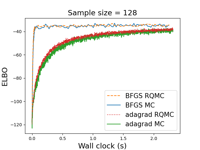
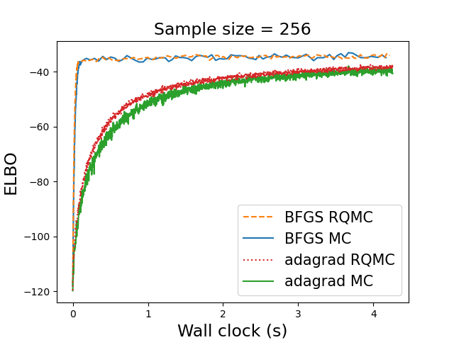
Figure 3: ELBO versus wall clock time in VB for Bayesian logistic regression. The methods and setup are described in the text. There are $n_{g}\in\{128,256\}$ gradient samples at each iteration and the second order methods use $n_{h}=1024$ Hessian samples every $B=20$’th iteration.

5.3 Crossed random effects

In this section, we consider a crossed random effects model. Both Bayesian and frequentist approaches to crossed random effects can be a challenge with costs scaling like $N^{3/2}$ or worse. See Papaspiliopoulos et al., (2020) and Ghosh et al., (2020) for Bayesian and frequentist approaches and also the dissertation of Gao, (2017).

An intercept only version of this model has

$$Y_{ij} \stackrel{{\scriptstyle\mathrm{ind}}}{{\sim}}\mathcal{N}(\mu+a_{i}+b_{j},1),\quad 1\leqslant i\leqslant I,\quad 1\leqslant j\leqslant J$$

given $\mu\sim\mathcal{N}(0,1)$, $a_{i}\,{\buildrel\text{iid}\over{\sim}\,}\mathcal{N}(0,\sigma_{a}^{2})$, and $b_{j}\,{\buildrel\text{iid}\over{\sim}\,}\mathcal{N}(0,\sigma_{b}^{2})$ where $\log\sigma_{a}$ and $\log\sigma_{b}$ are both $\mathcal{N}(0,1)$. All of $\mu$, $a_{i}$, $b_{j}$ and the log standard deviations are independent.

We use VB to approximate the posterior distribution of the $d=I+J+3$ dimensional parameter $\boldsymbol{z}=(\mu,\log\sigma_{a},\log\sigma_{b},\mathbf{a},\mathbf{b})$. In our example, we take $I=10$ and $J=5$. As before $q(\boldsymbol{z}\!\mid\!\theta)$ is chosen to be Gaussian with independent coordinates and $\theta$ has their means and standard deviations. In Figure 4, we plot the convergence of ELBO for different combinations of sampling methods and optimization methods. The BFGS method takes $B=20$, $M=30$, $n_{h}=512$. We used a learning rate of $0.01$ in AdaGrad. We observe that when the sample size is 8 (left), plain Monte Carlo has large fluctuations even when converged, especially for BFGS. When the sample size is 128 (right), the fluctuations disappear. But RQMC still achieves a higher ELBO than plain Monte Carlo for BFGS. In both cases, BFGS finds the optimum faster than AdaGrad.

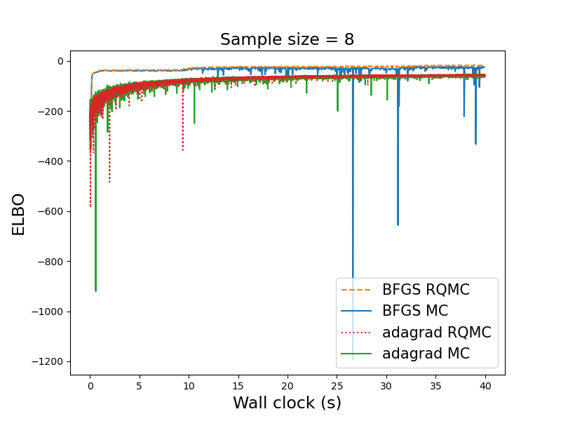
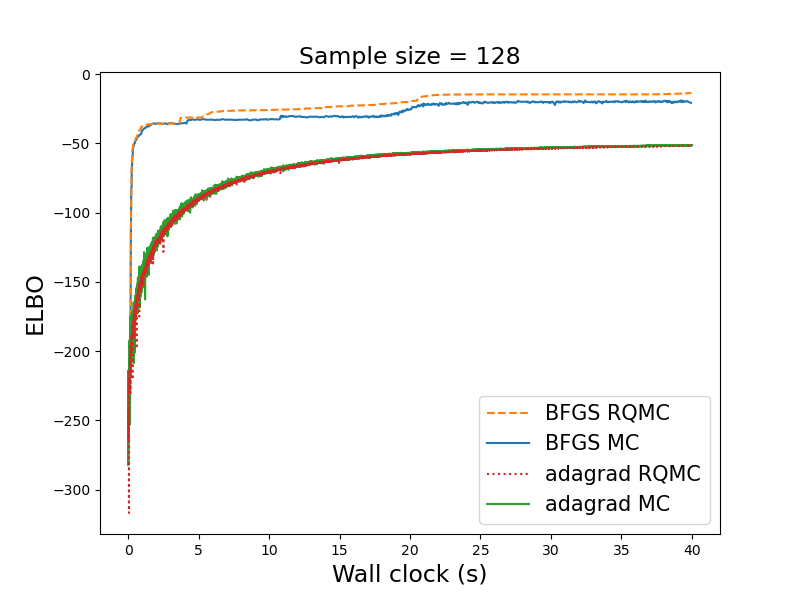
Figure 4: ELBO versus wall clock time in VB for crossed random effects. The methods and setup are described in the text. There are $n_{g}\in\{8,128\}$ gradient samples at each iteration.

5.4 Variational autoencoder

A variational autoencoder (VAE, Kingma and Welling, (2014)) learns a generative model for a dataset. A VAE has a probabilistic encoder and a probabilistic decoder. The encoder first produces a distribution $q_{\phi}(\boldsymbol{z}\!\mid\!\boldsymbol{x})$ over the latent variable $\boldsymbol{z}$ given a data point $\boldsymbol{x}$, then the decoder reconstructs a distribution $p_{\theta}(\boldsymbol{x}\!\mid\!\boldsymbol{z})$ over the corresponding $\boldsymbol{x}$ from the latent variable $\boldsymbol{z}$. The goal is to maximize the marginal probability $p_{\theta}(\boldsymbol{x})$. Observe that the ELBO provides a lower bound of $\log(p_{\theta}(\boldsymbol{x}))$:

$$\log p_{\theta}(\boldsymbol{x})-\mathcal{D}_{\mathrm{KL}}(q_{\phi}(\boldsymbol{z}\!\mid\!\boldsymbol{x})\,\|\,p_{\theta}(\boldsymbol{z}\!\mid\!\boldsymbol{x})) ={\mathbb{E}}_{\phi}(\log p_{\theta}(\boldsymbol{x}\!\mid\!\boldsymbol{z})\!\mid\!\boldsymbol{x})-\mathcal{D}_{\mathrm{KL}}(q_{\phi}(\boldsymbol{z}\!\mid\!\boldsymbol{x})\,\|\,p_{\theta}(z))=:{\mathcal{L}}(\theta,\phi\!\mid\!\boldsymbol{x}),$$

where ${\mathbb{E}}_{\phi}(\cdot\!\mid\!\boldsymbol{x})$ denotes expection for random $\boldsymbol{z}$ given $\boldsymbol{x}$ with parameter $\phi$. In this section $\boldsymbol{z}$ is the latent variable, and not a part of the ${\mathcal{Z}}$ that we use in our MC or RQMC algorithms. We do not refer to those variables in our VAE description below.

The usual objective is to maximize the ELBO $\sum_{i=1}^{N}{\mathcal{L}}(\theta,\phi\!\mid\!\boldsymbol{x}_{i})$ for a sample of $N$ IID $\boldsymbol{x}_{i}$ and now we have to optimize over $\phi$ as well as $\theta$. The first term ${\mathbb{E}}_{\phi}(\log p_{\theta}(\boldsymbol{x}\!\mid\!\boldsymbol{z}))$ in the ELBO is the reconstruction error, while the second term $\mathcal{D}_{\mathrm{KL}}(q_{\phi}(\boldsymbol{z}\!\mid\!\boldsymbol{x})\,\|\,p_{\theta}(z))$ penalizes parameters $\phi$ that give a posterior $q_{\phi}(\boldsymbol{z}\!\mid\!\boldsymbol{x})$ too different from the prior $p_{\theta}(\boldsymbol{z})$. Most commonly, $q_{\theta}(\boldsymbol{z}\!\mid\!\boldsymbol{x})=\mathcal{N}(\mu(\boldsymbol{x};\theta),\Sigma(\boldsymbol{x};\theta))$, and $p_{\theta}(\boldsymbol{z})=\mathcal{N}(0,I)$, so that the KL-divergence term $\mathcal{D}_{\mathrm{KL}}(q_{\phi}(\boldsymbol{z}\!\mid\!\boldsymbol{x})\,\|\,p_{\theta}(z))$ has a closed form. The decoding term $p_{\theta}(\boldsymbol{x}\!\mid\!\boldsymbol{z})$ is usually chosen to be a Gaussian or Bernoulli distribution, depending on the data type of $\boldsymbol{x}$. The expectation ${\mathbb{E}}_{\phi}({\log p_{\theta}(\boldsymbol{x}\!\mid\!\boldsymbol{z})\!\mid\!\boldsymbol{x}})$ is ordinarily estimated by MC. We implement both plain MC and RQMC in our experiments. To maximize the ELBO, the easiest way is to use SGD or its variants. We also compare SGD with L-BFGS in the experiments.

The experiment uses the MNIST dataset in PyTorch. It has 60,000 $28\times 28$ gray scale images, and so the dimension is 784. All experiments were conducted on a cluster node with 2 CPUs and 4GB memory. The training was conducted in a mini-batch manner with batch size 128. The encoder has a hidden layer with 800 nodes, and an output layer with 40 nodes, 20 for $\mu$ and 20 for $\sigma$. Our $\Sigma(\boldsymbol{x};\theta)$ takes the form ${\mathrm{diag}}(\sigma(\boldsymbol{x};\theta))$. The decoder has one hidden layer with 400 nodes.

In Figure 5(a), we plot the ELBO versus wall clock time for different combinations of sampling methods (MC, RQMC) and optimization methods (Adam, BFGS). The learning rate for Adam is 0.0001. For BFGS, the memory size is $M=20$. The other tuning parameters are set to the defaults from PyTorch. We observe that BFGS converged faster than Adam. For BFGS, we can also see that RQMC achieves a slightly higher ELBO than MC. Figure 5(b) through 5(e) shows some reconstructed images using the four algorithms.

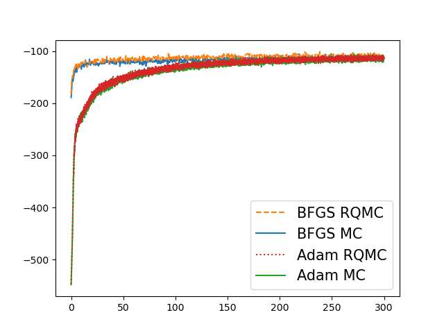
(a) ELBO

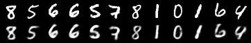
(b) BFGS RQMC

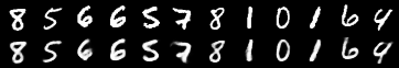
(c) BFGS MC

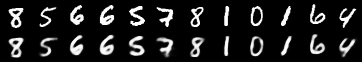
(d) Adam RQMC

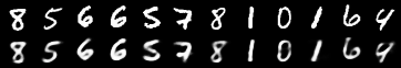
(e) Adam MC

Figure 5: Plot (a) shows the ELBO versus wall clock time for MC and RQMC used in both L-BFGS and Adam. Plots (b) through (e) show example images.

6 Discussion

RQMC methods are finding uses in simulation optimization problems in machine learning, especially in first order SGD algorithms. We have looked at their use in a second order, L-BFGS algorithm. RQMC is known theoretically and empirically to improve the accuracy in integration problems compared to both MC and QMC. We have shown that improved estimation of expected gradients translates directly into improved optimization for quasi-Newton methods. There is a small burden in reprogramming algorithms to use RQMC instead of MC, but that is greatly mitigated by the appearance of RQMC algorithms in tools such as BoTorch (Balandat et al.,, 2020) and the forthcoming scipy 1.7 (scipy.stats.qmc.Sobol) and QMCPy at https://pypi.org/project/qmcpy/.

Our empirical examples have used VB. The approach has potential value in Bayesian optimization (Frazier,, 2018) and optimal transport (El Moselhy and Marzouk,, 2012; Bigoni et al.,, 2016) as well.

The examples we chose were of modest scale where both first and second order methods could be used. In these settings, we saw that second order methods improve upon first order ones. For the autoencoder problem the second order methods converged faster than the first order ones did. This also happenend for the crossed random effects problem where the second order methods found better ELBOs than the first order ones did and RQMC-based quasi-Newton algorithm found a better ELBO than the MC-based quasi-Newton did without increasing the wall clock time.

It is possible that RQMC will bring an advantage to conjugate gradient approaches as they have some similarities to L-BFGS. We have not investigated them.

Appendix A Proof of main theorems

Our approach is similar to that used by Buchholz et al., (2018). They studied RQMC with SGD whereas we consider L-BFGS, a second order method.

A.1 Proof of Theorem 4.1

Proof  Let $e_{k}=\bar{g}({\mathcal{Z}}_{k};\theta_{k})-\nabla F(\theta_{k})$ be the error in estimating the gradient at step $k$. By the unbiasedness assumption, ${\mathbb{E}}(e_{k}\!\mid\!\theta_{k})=0$. Starting from the Lipschitz condition, we have

$$F(\theta_{k+1})-F(\theta_{k}) \leqslant\nabla F(\theta_{k})^{\intercal}(\theta_{k+1}-\theta_{k})+\frac{L}{2}\|\theta_{k+1}-\theta_{k}\|^{2}$$

$$=-\alpha_{k}\nabla F(\theta_{k})^{\intercal}H_{k}\bar{g}({\mathcal{Z}}_{k};\theta_{k})+\frac{L\alpha_{k}^{2}}{2}\|H_{k}\bar{g}({\mathcal{Z}}_{k};\theta_{k})\|^{2}$$

$$=-\alpha_{k}\nabla F(\theta_{k})^{\intercal}H_{k}e_{k}-\alpha_{k}\nabla F(\theta_{k})^{\intercal}{H_{k}}\nabla F(\theta_{k})$$

$$\qquad+\frac{L\alpha_{k}^{2}}{2}\left(\|H_{k}e_{k}\|^{2}+\|H_{k}\nabla F(\theta_{k})\|^{2}+2\nabla F(\theta_{k})^{\intercal}H_{k}^{2}e_{k}\right)$$

$$\leqslant-\alpha_{k}\nabla F(\theta_{k})^{\intercal}H_{k}e_{k}-\alpha_{k}h_{1}\|\nabla F(\theta_{k})\|^{2}$$

$$\qquad+\frac{L\alpha_{k}^{2}}{2}(h_{2}^{2}\|e_{k}\|^{2}+h_{2}^{2}\|\nabla F(\theta_{k})\|^{2}+2\nabla F(\theta_{k})^{\intercal}H_{k}^{2}e_{k})$$

$$=-\alpha_{k}\nabla F(\theta_{k})^{\intercal}H_{k}e_{k}+L\alpha_{k}^{2}\nabla F(\theta_{k})^{\intercal}H_{k}^{2}e_{k}$$

$$\qquad-\alpha_{k}h_{1}\Bigl{(}1-\frac{L\alpha_{k}h_{2}^{2}}{2h_{1}}\Bigr{)}\|\nabla F(\theta_{k})\|^{2}+\frac{L\alpha_{k}^{2}h_{2}^{2}}{2}\|e_{k}\|^{2}.$$

Because $\alpha_{k}=\alpha\leqslant{h_{1}}/({Lh_{2}^{2}})$, we have $1-{L\alpha_{k}h_{2}^{2}}/({2h_{1}})\geqslant 1/2$. Because strong convexity implies

$$\|\nabla F(\theta)\|^{2}\geqslant 2c(F(\theta)-F^{*}),\quad\forall\theta,$$

we have

$$F(\theta_{k+1})-F(\theta_{k}) \leqslant-\alpha_{k}\nabla F(\theta_{k})^{\intercal}(H_{k}-L\alpha_{k}H_{k}^{2})e_{k}-\alpha_{k}h_{1}c(F(\theta_{k})-F^{*})+\frac{L\alpha_{k}^{2}h_{2}^{2}}{2}\|e_{k}\|^{2}.$$

Adding $F(\theta_{k})-F^{*}$ to both sides gives

$$F(\theta_{k+1})-F^{*} \leqslant(1-\alpha_{k}h_{1}c)(F(\theta_{k})-F^{*})+R_{k},$$ (8)

where

$$R_{k}=-\alpha_{k}\nabla F(\theta_{k})^{\intercal}(H_{k}-L\alpha_{k}H_{k}^{2})e_{k}+\frac{L\alpha_{k}^{2}h_{2}^{2}}{2}\|e_{k}\|^{2}.$$

Let ${\mathcal{F}}_{k}=\sigma({\mathcal{Z}}_{i},1\leqslant i\leqslant k)$ be the filtration generated by the random inputs $\{{\mathcal{Z}}_{k}\}$ to our sampling process. Because ${\mathcal{Z}}_{k}$ are mutually independent and $H_{k}$ is independent of ${\mathcal{Z}}_{k}$, we have $\theta_{k},H_{k}\in{\mathcal{F}}_{k-1}$ and ${\mathbb{E}}(e_{k}\!\mid\!{\mathcal{F}}_{k-1})=0$. Then

$${\mathbb{E}}\bigl{(}\nabla F(\theta_{k})^{\intercal}(H_{k}-L\alpha_{k}H_{k}^{2})e_{k}\!\mid\!{\mathcal{F}}_{k-1}\bigr{)} =\nabla F(\theta_{k})^{\intercal}(H_{k}-L\alpha_{k}H_{k}^{2}){\mathbb{E}}(e_{k}\!\mid\!{\mathcal{F}}_{k-1})=0.$$

Therefore, $\nabla F(\theta_{k})^{\intercal}(H_{k}-L\alpha_{k}H_{k}^{2})e_{k}$ is a martingale difference sequence w.r.t. ${\mathcal{F}}_{k}$. Let

$$V_{k}={\mathbb{E}}(\|e_{k}\|^{2}\!\mid\!\theta_{k})={\mathrm{tr}}\bigl{(}\operatorname{Var}\left[\bar{g}({\mathcal{Z}}_{k};\theta_{k})\!\mid\!\theta_{k}\right]\bigr{)}.$$

Then $\|e_{k}\|^{2}-V_{k}$ is also a martingale difference sequence w.r.t. ${\mathcal{F}}_{k}$. So we can write

$$R_{k}=\nu_{k}+\frac{L\alpha_{k}^{2}h_{2}^{2}}{2}V_{k},$$

where

$$\nu_{k}=-\alpha_{k}\nabla F(\theta_{k})^{\intercal}(H_{k}-L\alpha_{k}H_{k}^{2})e_{k}+\frac{L\alpha_{k}^{2}h_{2}^{2}}{2}(\|e_{k}\|^{2}-V_{k})$$

is a martingale difference sequence, and ${L\alpha_{k}^{2}h_{2}^{2}}/({2}V_{k})$ is a deterministic sequence. Recursively applying equation (8) gives

$$F(\theta_{K})-F^{*} \leqslant(1-\alpha ch_{1})^{K}(F(\theta_{0})-F^{*})+\sum_{k=0}^{K-1}(1-\alpha ch_{1})^{K-k-1}R_{k}$$

$$=(1-\alpha ch_{1})^{K}(F(\theta_{0})-F^{*})+\sum_{k=0}^{K-1}(1-\alpha ch_{1})^{K-k-1}\Bigl{(}\nu_{k}+\frac{L\alpha^{2}h_{2}^{2}}{2}V_{k}\Bigr{)}.$$

By the bounded variance assumption, $V_{k}\leqslant M$ for all $k\geqslant 0$. Hence,

$$F(\theta_{K})-F^{*} \leqslant(1-\alpha c)^{K}(F(\theta_{0})-F^{*})+\frac{\alpha Lh_{2}^{2}}{2ch_{1}}M+\sum_{k=0}^{K-1}(1-\alpha ch_{1})^{K-k-1}\nu_{k}.$$

Taking expectations on both sides proves (6).

To prove the finite sample guarantee (7), it remains to bound the martingale $\sum_{k=0}^{K-1}(1-\alpha ch_{1})^{K-k-1}\nu_{k}$ with high probability. We assumed a bound on $\|g(\boldsymbol{z};\theta)\|$ which implies one for $\|\bar{g}({\mathcal{Z}};\theta)\|$ as well for any fixed $n$. When the norms of the gradient $\nabla F(\theta)$ and gradient estimator $\bar{g}({\mathcal{Z}};\theta)$ are bounded by such a constant $C$ for all $\theta$ and ${\mathcal{Z}}$, then $\|e_{k}\|=\|\bar{g}({\mathcal{Z}};\theta)-\nabla F(\theta)\|\leqslant 2C$, and we have the bound

$$|\nu_{k}|\leqslant\alpha|\nabla F(\theta_{k})^{\intercal}(H_{k}-L\alpha H_{k}^{2})e_{k}|+\frac{L\alpha^{2}h_{2}^{2}}{2}C^{2}\leqslant 2\alpha(h_{2}-L\alpha h_{1}^{2}+{L\alpha h_{2}^{2}})C^{2}=:C^{\prime},$$

where the second inequality uses that the largest eigenvalue of $H_{k}-L\alpha H_{k}^{2}$ is upper bounded by $h_{2}-L\alpha h_{1}^{2}$. By the Azuma-Hoeffding inequality (Azuma,, 1967), for all $t\geqslant 0$,

$$\mathbb{P}\biggl{(}\,{\sum_{k=1}^{K}(1-\alpha ch_{1})^{K-k-1}\nu_{k}\geqslant t}\biggr{)}\leqslant\exp\biggl{(}{-\frac{2t^{2}}{\sum_{k=1}^{K}(1-\alpha ch_{1})^{K-k-1}C^{\prime 2}}}\biggr{)}\leqslant\exp\biggr{(}{-\frac{2t^{2}}{\frac{C^{\prime 2}}{\alpha ch_{1}}}}\biggr{)}.$$

Setting $\varepsilon^{2}={2t^{2}\alpha ch_{1}}/{C^{\prime 2}}$ gives

$$t=\frac{C^{\prime}}{\sqrt{2\alpha ch_{1}}}\varepsilon=\frac{2\alpha C^{2}(h_{2}-L\alpha h_{1}^{2}+{L\alpha h_{2}^{2}})}{\sqrt{2\alpha ch_{1}}}\varepsilon\leqslant C^{2}\sqrt{\frac{2\alpha}{ch_{1}}}(h_{2}-L\alpha h_{1}^{2}+{h_{1}}{})\varepsilon.$$

So we have proved that with probability at least $1-e^{-\varepsilon^{2}}$,

$$F(\theta_{K})-F^{*} \leqslant(1-\alpha ch_{1})^{K}(F(\theta_{0})-F^{*})+\frac{\alpha Lh_{2}^{2}}{2ch_{1}}M+C^{2}\sqrt{\frac{2\alpha}{ch_{1}}}(h_{2}-L\alpha h_{1}^{2}+{h_{1}}{})\varepsilon.$$

 

A.2 Proof of Theorem 4.2

Our proof uses the following lemma.

Lemma 1

Let $u,v\in^{n}$ satisfy $u^{\intercal}v\geqslant A$ and let $D\in^{n\times n}$ be symmetric with $h_{1}I\preccurlyeq D\preccurlyeq h_{2}I$ where $0<h_{1}\leqslant h_{2}$. Then

$$u^{\intercal}Dv\geqslant\frac{h_{1}+h_{2}}{2}A-\frac{h_{2}-h_{1}}{2}\|u\|\|v\|.$$

Proof  Without loss of generality, we can assume that $D$ is a diagonal matrix. Otherwise, let $D=U\Lambda U^{\intercal}$ be the eigen-decomposition of $D$. Then $u^{\intercal}Dv=(U^{\intercal}u)^{\intercal}\Lambda(U^{\intercal}v)$, $\|U^{\intercal}u\|=\|u\|$, $\|U^{\intercal}v\|=\|v\|$, and $(U^{\intercal}u)^{\intercal}(U^{\intercal}v)=u^{\intercal}v$, and we can replace $D$ by $\Lambda$.

Let $d_{1},\ldots,d_{n}$ be the diagonal entries of $D$. Then $u^{\intercal}Dv=\sum_{i=1}^{n}u_{i}v_{i}d_{i}$. Let $s_{+}=\sum_{i:u_{i}v_{i}\geqslant 0}u_{i}v_{i}$ and $s_{-}=\sum_{i:u_{i}v_{i}<0}u_{i}v_{i}$. Note that $s_{+}+s_{-}=u^{\intercal}v\geqslant A$, $s_{+}-s_{-}=\sum_{i=1}^{n}|u_{i}v_{i}|\leqslant\|u\|\|v\|$. Then for any $D$,

$$u^{\intercal}Dv\geqslant h_{1}s_{+}+h_{2}s_{-}=\frac{h_{1}+h_{2}}{2}(s_{+}+s_{-})+\frac{h_{2}-h_{1}}{2}(s_{-}-s_{+})\geqslant\frac{h_{1}+h_{2}}{2}A-\frac{h_{2}-h_{1}}{2}\|u\|\|v\|.$$

 

Now we are ready to prove Theorem 4.2.

Proof  We start by decomposing

$$\|\theta_{k+1}-\theta^{*}\|^{2} =\|\theta_{k+1}-\theta_{k}+\theta_{k}-\theta^{*}\|^{2}$$

$$=\|\theta_{k}-\theta^{*}\|^{2}+\alpha^{2}\|H_{k}\bar{g}({\mathcal{Z}}_{k};\theta_{k})\|^{2}-2\alpha(\theta_{k}-\theta^{*})^{\intercal}H_{k}\bar{g}({\mathcal{Z}}_{k};\theta_{k}).$$

Note that only $\bar{g}({\mathcal{Z}}_{k};\theta_{k})$ and $\theta_{k+1}$ depend on ${\mathcal{Z}}_{k}$. Taking expectation w.r.t. ${\mathcal{Z}}_{k}$ on both sides gives

$${\mathbb{E}}\bigl{(}\|\theta_{k+1}-\theta^{*}\|^{2}\bigr{)} \leqslant\|\theta_{k}-\theta^{*}\|^{2}+\alpha^{2}h_{2}^{2}(M+\|\nabla F(\theta_{k})\|^{2})-2\alpha(\theta_{k}-\theta^{*})^{\intercal}H_{k}\nabla F(\theta_{k})$$

$$\leqslant\|\theta_{k}-\theta^{*}\|^{2}+\alpha^{2}h_{2}^{2}(M+L^{2}\|\theta_{k}-\theta^{*}\|^{2})-2\alpha(\theta_{k}-\theta^{*})^{\intercal}H_{k}\nabla F(\theta_{k}).$$ (9)

By strong convexity of $F(\cdot)$,

$$(\theta_{k}-\theta^{*})^{\intercal}\nabla F(\theta_{k})\geqslant F(\theta_{k})-F^{*}+\frac{c}{2}\|\theta_{k}-\theta^{*}\|^{2}\geqslant c\|\theta_{k}-\theta^{*}\|^{2}.$$

Using Lemma 1 and equation (A.2), we have

$$(\theta_{k}-\theta^{*})^{\intercal}H_{k}\nabla F(\theta_{k}) \geqslant\frac{h_{1}+h_{2}}{2}c\|\theta_{k}-\theta^{*}\|^{2}-\frac{h_{2}-h_{1}}{2}\|\theta_{k}-\theta^{*}\|\|\nabla F(\theta_{k})\|$$

$$\geqslant\Bigl{(}\frac{h_{1}+h_{2}}{2}c-\frac{h_{2}-h_{1}}{2}L\Bigr{)}\|\theta_{k}-\theta^{*}\|^{2},$$

where the last inequality is due to $\|\nabla F(\theta_{k})\|\leqslant L\|\theta_{k}-\theta^{*}\|$. Combining this with (9) gives

$${\mathbb{E}}\bigl{(}{\|\theta_{k+1}-\theta^{*}\|^{2}}\bigr{)} \leqslant\bigl{(}1+\alpha^{2}L^{2}h_{2}^{2}-\alpha[(h_{1}+h_{2})c-(h_{2}-h_{1})L]\bigr{)}\|\theta_{k}-\theta^{*}\|^{2}+\alpha^{2}h_{2}^{2}M.$$

We have assumed that

$$0<\alpha<\frac{(h_{1}+h_{2})c-(h_{2}-h_{1})L}{2L^{2}h_{2}^{2}}$$

and it then follows that

$$\bigl{(}1+\alpha^{2}L^{2}h_{2}^{2}-\alpha[(h_{1}+h_{2})c-(h_{2}-h_{1})L]\bigr{)}\leqslant 1-\alpha^{2}h_{2}^{2}L^{2}$$

from which

$${\mathbb{E}}\bigl{(}{\|\theta_{k+1}-\theta^{*}\|^{2}}\bigr{)} \leqslant\bigl{(}1-\alpha^{2}h_{2}^{2}L^{2}\bigr{)}\|\theta_{k}-\theta^{*}\|^{2}+\alpha^{2}h_{2}^{2}M.$$ (11)

Applying the recursive error formula (11) we get

$${\mathbb{E}}\bigl{(}\|\theta_{k}-\theta^{*}\|^{2}\bigr{)}\leqslant(1-\alpha^{2}h_{2}^{2}L^{2})^{k}\|\theta_{0}-\theta^{*}\|^{2}+\frac{M}{L^{2}}.$$

where the expectation is over ${\mathcal{Z}}_{1},\dots,{\mathcal{Z}}_{k}$.

References

• Agarwal etΒ al., (2012) Agarwal, A., Bartlett, P.Β L., Ravikumar, P., and Wainwright, M.Β J. (2012). Information-theoretic lower bounds on the oracle complexity of stochastic convex optimization. IEEE Transactions on Information Theory, 58(5):3235–3249.
• AndradΓ³ttir, (1998) AndradΓ³ttir, S. (1998). A review of simulation optimization techniques. In 1998 winter simulation conference, volumeΒ 1, pages 151–158. IEEE.
• Azuma, (1967) Azuma, K. (1967). Weighted sums of certain dependent random variables. Tohoku Mathematical Journal, Second Series, 19(3):357–367.
• Balandat etΒ al., (2020) Balandat, M., Karrer, B., Jiang, D.Β R., Daulton, S., Letham, B., Wilson, A.Β G., and Bakshy, E. (2020). BoTorch: A Framework for Efficient Monte-Carlo Bayesian Optimization. In Advances in Neural Information Processing Systems 33.
• Basu and Mukherjee, (2017) Basu, K. and Mukherjee, R. (2017). Asymptotic normality of scrambled geometric net quadrature. Annals of Statistics, 45(4):1759–1788.
• Beck, (2017) Beck, A. (2017). First-order methods in optimization. SIAM, Philadelphia.
• Berahas etΒ al., (2016) Berahas, A.Β S., Nocedal, J., and TakÑč, M. (2016). A multi-batch L-BFGS method for machine learning. Advances in Neural Information Processing Systems, pages 1063–1071.
• Bigoni etΒ al., (2016) Bigoni, D., Spantini, A., and Marzouk, Y. (2016). Adaptive construction of measure transports for Bayesian inference. In NIPS workshop on Approximate Inference.
• Blei etΒ al., (2017) Blei, D.Β M., Kucukelbir, A., and McAuliffe, J.Β D. (2017). Variational inference: A review for statisticians. Journal of the American Statistical Association, 112(518):859–877.
• Bollapragada etΒ al., (2018) Bollapragada, R., Nocedal, J., Mudigere, D., Shi, H.Β J., and Tang, P. T.Β P. (2018). A progressive batching L-BFGS method for machine learning. In International Conference on Machine Learning, pages 620–629. PMLR.
• Bottou etΒ al., (2018) Bottou, L., Curtis, F.Β E., and Nocedal, J. (2018). Optimization methods for large-scale machine learning. Siam Review, 60(2):223–311.
• Buchholz etΒ al., (2018) Buchholz, A., Wenzel, F., and Mandt, S. (2018). Quasi-Monte Carlo variational inference. In International Conference on Machine Learning, pages 668–677. PMLR.
• Byrd etΒ al., (2016) Byrd, R.Β H., Hansen, S.Β L., Nocedal, J., and Singer, Y. (2016). A stochastic quasi-Newton method for large-scale optimization. SIAM Journal on Optimization, 26(2):1008–1031.
• Caflisch etΒ al., (1997) Caflisch, R.Β E., Morokoff, W., and Owen, A.Β B. (1997). Valuation of mortgage backed securities using Brownian bridges to reduce effective dimension. Journal of Computational Finance, 1(1):27–46.
• Chen etΒ al., (2014) Chen, W., Srivastav, A., and Travaglini, G., editors (2014). A panorama of discrepancy theory. Springer, Cham, Switzerland.
• Cranley and Patterson, (1976) Cranley, R. and Patterson, T. N.Β L. (1976). Randomization of number theoretic methods for multiple integration. SIAM Journal of Numerical Analysis, 13(6):904–914.
• Devroye, (1986) Devroye, L. (1986). Non-uniform Random Variate Generation. Springer, New York.
• Dick etΒ al., (2013) Dick, J., Kuo, F.Β Y., and Sloan, I.Β H. (2013). High-dimensional integration: the quasi-Monte Carlo way. Acta Numerica, 22:133–288.
• Dick and Pillichshammer, (2010) Dick, J. and Pillichshammer, F. (2010). Digital sequences, discrepancy and quasi-Monte Carlo integration. Cambridge University Press, Cambridge.
• Duchi etΒ al., (2011) Duchi, J., Hazan, E., and Singer, Y. (2011). Adaptive subgradient methods for online learning and stochastic optimization. Journal of Machine Learning Research, 12(7).
• Duchi, (2018) Duchi, J.Β C. (2018). Introductory lectures on stochastic optimization. In Mahoney, M.Β W., Duchi, J.Β C., and Gilbert, A.Β C., editors, The mathematics of data, volumeΒ 25, pages 99–186. American Mathematical Society, Providence, RI.
• ElΒ Moselhy and Marzouk, (2012) ElΒ Moselhy, T.Β A. and Marzouk, Y.Β M. (2012). Bayesian inference with optimal maps. Journal of Computational Physics, 231(23):7815–7850.
• Faure, (1982) Faure, H. (1982). DiscrΓ©pance de suites associΓ©es Γ  un systΓ¨me de numΓ©ration (en dimension $s$). Acta Arithmetica, 41:337–351.
• Frazier, (2018) Frazier, P.Β I. (2018). A tutorial on Bayesian optimization. Technical report, arXiv:1807.02811.
• Gao, (2017) Gao, K. (2017). Scalable Estimation and Inference for Massive Linear Mixed Models with Crossed Random Effects. PhD thesis, Stanford University.
• Ghosh etΒ al., (2020) Ghosh, S., Hastie, T., and Owen, A.Β B. (2020). Backfitting for large scale crossed random effects regressions. Technical report, arXiv:2007.10612.
• Gower etΒ al., (2016) Gower, R., Goldfarb, D., and RichtΓ‘rik, P. (2016). Stochastic block BFGS: Squeezing more curvature out of data. In International Conference on Machine Learning, pages 1869–1878.
• Joe and Kuo, (2008) Joe, S. and Kuo, F.Β Y. (2008). Constructing Sobol’ sequences with better two-dimensional projections. SIAM Journal on Scientific Computing, 30(5):2635–2654.
• Johnson and Zhang, (2013) Johnson, R. and Zhang, T. (2013). Accelerating stochastic gradient descent using predictive variance reduction. In Advances in Neural Information Processing Systems, volumeΒ 26, pages 315–323.
• Kingma and Ba, (2014) Kingma, D.Β P. and Ba, J. (2014). Adam: A method for stochastic optimization. Technical report, arXiv:1412.6980.
• Kingma and Welling, (2014) Kingma, D.Β P. and Welling, M. (2014). Auto-encoding variational Bayes. stat, 1050:1.
• L’Ecuyer and Lemieux, (2002) L’Ecuyer, P. and Lemieux, C. (2002). A survey of randomized quasi-Monte Carlo methods. In Dror, M., L’Ecuyer, P., and Szidarovszki, F., editors, Modeling Uncertainty: An Examination of Stochastic Theory, Methods, and Applications, pages 419–474. Kluwer Academic Publishers.
• Loh, (2003) Loh, W.-L. (2003). On the asymptotic distribution of scrambled net quadrature. Annals of Statistics, 31(4):1282–1324.
• Miller etΒ al., (2017) Miller, A.Β C., Foti, N.Β J., DΒ Amour, A., and Adams, R.Β P. (2017). Reducing reparameterization gradient variance. In Advances in Neural Information Processing Systems.
• Mohamed etΒ al., (2020) Mohamed, S., Rosca, M., Figurnov, M., and Mnih, A. (2020). Monte Carlo gradient estimation in machine learning. Journal of Machine Learning Research, 21(132):1–62.
• Moritz etΒ al., (2016) Moritz, P., Nishihara, R., and Jordan, M. (2016). A linearly-convergent stochastic L-BFGS algorithm. In Artificial Intelligence and Statistics, pages 249–258.
• Niederreiter, (1992) Niederreiter, H. (1992). Random Number Generation and Quasi-Monte Carlo Methods. SIAM, Philadelphia, PA.
• Nocedal, (1980) Nocedal, J. (1980). Updating quasi-Newton matrices with limited storage. Mathematics of computation, 35(151):773–782.
• Nocedal and Wright, (2006) Nocedal, J. and Wright, S. (2006). Numerical Optimization. Springer Science & Business Media, New York, second edition.
• Owen, (1995) Owen, A.Β B. (1995). Randomly permuted (t,m,s)π‘‘π‘šπ‘ (t,m,s)-nets and $(t,s)$-sequences. In Niederreiter, H. and Shiue, P. J.-S., editors, Monte Carlo and Quasi-Monte Carlo Methods in Scientific Computing, pages 299–317, New York. Springer-Verlag.
• (41) Owen, A.Β B. (1997a). Monte Carlo variance of scrambled net quadrature. SIAM Journal of Numerical Analysis, 34(5):1884–1910.
• (42) Owen, A.Β B. (1997b). Scrambled net variance for integrals of smooth functions. Annals of Statistics, 25(4):1541–1562.
• Owen, (2005) Owen, A.Β B. (2005). Multidimensional variation for quasi-Monte Carlo. In Fan, J. and Li, G., editors, International Conference on Statistics in honour of Professor Kai-Tai Fang’s 65th birthday.
• Owen, (2008) Owen, A.Β B. (2008). Local antithetic sampling with scrambled nets. Annals of Statistics, 36(5):2319–2343.
• Owen and Rudolf, (2021) Owen, A.Β B. and Rudolf, D. (2021). A strong law of large numbers for scrambled net integration. SIAM Review, 63(2):360–372.
• Paisley etΒ al., (2012) Paisley, J., Blei, D.Β M., and Jordan, M.Β I. (2012). Variational Bayesian inference with stochastic search. In Proceedings of the 29th International Coference on International Conference on Machine Learning, pages 1363–1370.
• Papaspiliopoulos etΒ al., (2020) Papaspiliopoulos, O., Roberts, G.Β O., and Zanella, G. (2020). Scalable inference for crossed random effects models. Biometrika, 107(1):25–40.
• Shi etΒ al., (2020) Shi, H.Β J., Xie, Y., Byrd, R., and Nocedal, J. (2020). A noise-tolerant quasi-Newton algorithm for unconstrained optimization. Technical report, arXiv:2010.04352.
• Sobol’, (1969) Sobol’, I.Β M. (1969). Multidimensional Quadrature Formulas and Haar Functions. Nauka, Moscow. (In Russian).
• Xie etΒ al., (2020) Xie, Y., Byrd, R.Β H., and Nocedal, J. (2020). Analysis of the BFGS method with errors. SIAM Journal on Optimization, 30(1):182–209.
• Yue and Mao, (1999) Yue, R.-X. and Mao, S.-S. (1999). On the variance of quadrature over scrambled nets and sequences. Statistics & probability letters, 44(3):267–280.