∎
11institutetext: E. Padway 22institutetext: National Institute of Aerospace, 100 Exploration Way, Hampton, VA, 23666
22email: emmett.padway@nianet.org 33institutetext: D. Mavriplis 44institutetext: University of Wyoming, Department of Mechanical Engineering, 1000 E. University Ave, Laramie, WY, 82071
Approximate Linearization of Fixed Point Iterations
Abstract
Previous papers have shown the impact of partial convergence of discretized PDEs on the accuracy of tangent and adjoint linearizations. A series of papers suggested linearization of the fixed point iteration used in the solution process as a means of computing the sensitivities rather than linearizing the discretized PDE, as the lack of convergence of the nonlinear problem indicates that the discretized form of the governing equations has not been satisfied. These works showed that the accuracy of an approximate linearization depends in part on the convergence of the nonlinear system. This work shows an error analysis of the impact of the approximate linearization and the convergence of the nonlinear problem for both the tangent and adjoint modes and provides a series of results for an exact Newton solver, an inexact Newton solver, and a low storage explicit Runge-Kutta scheme to confirm the error analyses.
Keywords:
Fixed point iterations discrete adjoint gradients computational fluid dynamics optimization1 Introduction
Tangent and Adjoint methods have become a larger part of the field of Computational Fluid Dynamics (CFD) as computers and algorithms have developed and a concurrent push for automatic design has strengthened. Both of these methods are derived from the requirement that the discretized form of the governing Partial Differential Equations (PDE) is satisfied; for steady state problems this is characterized by the magnitude of the residual vector of the spatially discretized terms approaching machine zero. The adjoint linearization (either through the discrete or continuous methods) is more commonly used as it scales independent of the number of design variables and is used for error estimation MAMN ; DDAMR . These methods are highly accurate and are often verified through use of the complex-step finite-difference method as this does not suffer from round off error SKN_Thesis . However, for cases where the discretized governing equations are not satisfied, the complex-step finite-difference method gives the sensitivity of the solution process and both the adjoint and tangent linearizations are no longer exact linearizations with the adjoint losing duality to the primal problem. Such cases have been shown to be very common in CFD simulations JKDD ; JKQW ; PTA-devel and in such cases the sensitivities suffer greatly in terms of accuracy and exhibit a high dependence on the state of the simulation at termination.
To address these cases Padway and Mavriplis PTA-devel ; PTA-iqn investigated linearizing the fixed point iteration used to solve the nonlinear problem and obtained the sensitivities of the solution process. Through this method they showed better sensitivity behavior and successful optimizations; they also applied this method to error estimation and adaptive mesh refinement PTA-amr . This method inherits some of the characteristics shown in the work on one-shot optimization methods OneShotOpt including the guaranteed convergence of the tangent and adjoint problems, due to their similarity to the black box approach BB_Sagebaum . Padway and Mavriplis PTA-iqn showed by numerical experiment that for an approximately linearized quasi-Newton fixed point iteration, convergence of the non-linear problem led to a decrease in error from the approximate linearization. The issue of inexact linearization of a linear system solve has been investigated previously to produce consistent automatic differentiation of linear system solves in segregated solvers JDM_LinAlg . These linearizations would be necessary in the ”piggy-back” iterations of the one-shot adjoint method OSA_Gunther when applied to implicit nonlinear solvers. In this paper the authors show through a series of proofs and numerical experiments, that – providing the residual operator is linearized exactly – the error from inexact linearization of the fixed point iteration approaches 0 at the same rate of the nonlinear problem convergence, a necessary condition for approximate linearizations to be useful in applications. Additionally, the authors show that for nonconverged problems, the error in the sensitivity has two terms, one of which scales with the residual, and the other of which scales with the error in the approximate linearization; the second of which is multiplied by the derivative of the contractive fixed point iteration; a discovery that allows a user to select the level of error they desire in their sensitivities. Additionally, this allows users to know that by converging the nonlinear problem they can obtain greater accuracy in the sensitivities despite the inaccuracy of the approximate linearization of the fixed point iteration. As problems with nonconvergent fixed points have become more prevalent as the field has attempted more difficult problems, methods like those mentioned above show more promise. In the realm of design optimization, which is the focus of this paper, inaccurate adjoints can lead to inaccurate sensitivities, which can change the course of the design cycle and lead to stagnation; as the Karush-Kuhn-Tucker (KKT) conditions, which govern termination, require that the gradient vanish at a local extremum SNopt2 . As such having a good estimate on the error of the sensitivities for such a method (when compared to the complex-step finite-difference method) that can provide better designs than those provided by the solution of the classical steady-state adjoint is highly desirable. In a similar vein, Brown and Nadarajah SKN investigate a bound for the error in the adjoint computed sensitivities arising from partial convergence of the primal problem for problems that show smooth convergence behavior.
This paper is organized as follows. We first consider the details of the CFD solver used in this work, explaining the discretization, the solution methodologies, and the classical steady-state adjoint and tangent problems. Then we show the pseudo-time accurate tangent and adjoint linearizations to obtain design sensitivities along with a discussion of the approximation decisions. After which we show analyses of the error in the design sensitivities of both linearizations. We then show numerical results for sensitivity computations for an airfoil in transonic flow, thus confirming the analyses and showing that these analyses hold for both explicit and implicit solvers.
2 Background and In-House Solver
2.1 Governing Equations
We developed an in-house flow solver to solve the steady-state Euler equations on unstructured meshes. The steady-state compressible Euler equations (which may also be referred to as the primal or analysis problem) can be written as follows:
| (1) |
where is the conservative variable vector, is the design variable vector, and is the conservative variable flux. Equation (1) can also be written as:
| (2) |
where R is the residual operator.
2.2 Spatial Discretization
The residual about the closed control volume is given as
| (3) |
this is the operator in the aforementioned requirement for the adjoint and tangent systems. In the discretized form of the residual operator, is a given edge of the triangulation, is the number of edges in the triangulation, is the element boundary, is the mesh point coordinate vector, is the numerical flux across the element boundary, and is the edge normal on the element boundary. The solver used in this work is a steady-state finite-volume cell-centered Euler solver with second-order spatial accuracy for triangular elements. Second-order accuracy is implemented through weighted least squares gradient reconstruction LSQR . The solver has three different flux calculations implemented and linearized, these are the Lax-FriedrichsLF , RoeRoe , and Van LeerVL schemes. In this work, only the Van-Leer scheme is used due to the suitability of the results at a decreased expense and increased stability when compared to the Roe flux.
2.3 Steady-State Solver
To solve the discretized PDE shown above we define a fixed point iteration (N):
| (4) | ||||
where is the solution increment (also referred to as ), is an operator that defines the nonlinear solver and is the vector of mesh point coordinates in the triangulation which is a function of the design variable vector (often a parameterization) held fixed at each design iteration. The solver technology for this code uses either explicit pseudo-time stepping with a forward Euler scheme or a low storage five stage Runge-Kutta scheme, or implicit pseudo-time stepping with a quasi-Newton method. The quasi-Newton method is implemented using pseudo-transient continuation (PTC) with a BDF1 pseudo temporal discretization scheme. For Newton’s method the time-stepping procedure is written as:
| (5) |
where we compute by solving the following system of linear equations.
| (6) |
where denotes a left hand matrix that determines the nonlinear solver. If is the exact linearization of the residual operator this is an exact Newton solver; otherwise we recover an inexact-quasi-Newton solver of which the most typical matrix is the linearization of a lower order discretization with a pseudo-time term. We can substitute the expression for into the time-stepping equation (5) to obtain the final form of this equation
| (7) |
Here is the Jacobian of the first order spatial discretization augmented with a diagonal term to ensure that it is diagonally dominant, shown in equation (8). The use of the Jacobian of the first-order spatial discretization turns this into an inexact-quasi-Newton solver, which is often used due to the robustness and ease of implementation when compared to the Jacobian of a second-order discretization. This is especially desirable in this work because the inspiration behind the methods that are analyzed herein are methods used for optimization or error esimation where the flow solver does not converge and the added robustness is desired.
| (8) |
where is the volume (or area) of the element, is the CFL number at the given iteration and is a local time step given as:
| (9) |
Here is the circumference of the inscribed circle for mesh cell , and are the horizontal and vertical velocity components respectively, and is the speed of sound in the triangular element. Please note the subscript on the Jacobian in equation (8) denotes that it is the Jacobian of the first order accurate spatial discretization; the subscript of 2 would indicate the Jacobian of the second order accurate discretization, and that for the above definition of the operator this would imply:
| (10) |
Furthermore, the CFL is scaled either with a simple ramping coefficient () and cap criterion:
| (11) |
or with a line search and CFL controller DJMLS ; BALS , which seeks to minimize the norm of the pseudo-temporal residual, defined as:
| (12) |
In order to solve the linear system that arises in the quasi-Newton method we use a flexible GMRES solver GMRES preconditioned by Gauss-Seidel iterations or the Gauss-Seidel iterations alone. The flexible GMRES solver is also used to solve the stiff steady state tangent and adjoint systems as well.
2.4 A Review of Tangent and Adjoint Systems
2.4.1 Tangent Formulation
For an aerodynamic optimization problem, we consider an objective functional , for example lift or drag. In order to obtain an expression for the sensitivities we take the derivative of the objective functional mavriplis_vki :
| (13) |
For the above expression and can be directly obtained by differentiating the corresponding subroutines in the code and is dependent on the choice of mesh motion scheme and design variables. It is not possible to obtain through linearization of the subroutines in the code without linearizing the entire analysis solution process, as will be covered in later sections. In order to solve for this term we use the constraint that for a fully converged flow . By taking the derivative of the residual operator we obtain the equation below:
| (14) |
We can isolate the sensitivity of the residual to the design variables to obtain the tangent system:
| (15) |
We solve this linear system, using hand differentiated subroutines to provide the left hand matrix , the right hand side (which scales with the design variables), and obtain . We then substitute into equation (13) to obtain the final sensitivities.
2.4.2 Discrete Adjoint Formulation
The adjoint formulation begins with the same sensitivity equation:
| (16) |
Using the condition , we return to equation (15) and pre-multiply both sides of the equation by the inverse Jacobian matrix to obtain:
| (17) |
Substituting the above expression into the sensitivity equation yields:
| (18) |
We then define an adjoint variable such that:
| (19) |
which gives an equation for the adjoint variable:
| (20) |
We can solve this linear system and obtain the sensitivities for the objective function as follows:
| (21) |
The adjoint system is of interest, because as mentioned in the introduction, it results in an equation for the sensitivity that does not scale with the number of design variables.
3 Development of the Pseudo-Time Accurate Tangent
In this section we show the previously derived pseudo-time accurate tangent formulations PTA-devel ; PTA-iqn . We also discuss the impacts on implementation and accuracy of some of the assumptions made in the previous formulation; the assumptions are exact when the linear system at each iteration is solved to machine precision. In such cases the tangent sensitivities would exactly correspond to the sensitivities of solution process itself, and would correspond exactly to the sensitivities obtained by the complex-step finite difference method at each step of the solution process. We note that in this section and the derivation of the adjoint section, when taking the derivative of an operator with respect to the design variables, is an abbreviation of .
3.1 Tangent System for quasi-Newton Method
Previous works on the pseudo-time accurate adjoint PTA-devel ; PTA-iqn have contained investigations on the desireability of an objective function averaged in pseudo-time over the last steps, expressed as:
| (22) |
The sensitivity equation for such a problem is
| (23) |
In this work we focus on objective functions calculated only at the final iteration/pseudo-time step; such a decision greatly simplifies the analyses and they can still be straightforwardly extended to multiple iteration objective functions. We recover
| (24) |
which is identical to the sensitivity equation of the steady state tangent system (13). For this section, we begin from equation (7)
| (25) |
where is again a first-order accurate Jacobian augmented with a diagonal term to ensure that it is diagonally dominant, as described in equation (8):
| (26) |
If we take the derivative of each side of equation (25) we obtain:
| (27) | ||||
Here, rather than neglecting the change in the preconditioner we use a definition of the derivative of the matrix inverse defined by:
| (28) |
as applied in previous work PTA-iqn . This assumption will not be exact for any case in which the linear system solution is not exact to machine precision. However, it will allow us to have a clearly defined source of error in a computation and evaluate how much the linear tolerance of the system affects the sensitivity computation. Such an investigation was not done in the previous work, but is the thrust of this paper, and the effect of this approximation will be examined, as well as an investigation into the behavior of other approximate linearizations. By computing the total derivative of the nonlinear solver– as in equation(27)– and applying (28) with into equation (27), the below expression is generated:
| (29) | ||||
Expanding the total derivative shows that this is in fact the sum of two matrix vector products:
| (30) | ||||
While the full hessian is an undesireable item to compute, this formulation requires two hessian vector products that can be obtained through complex perturbations to the conservative variables and nodal coordinate vectors, and subsequent evaluation of the Jacobian. This use of Frechét differentiation obviates the need for the full hessian computation. Furthermore, one of the matrix inverses can be removed by reusing the computation of in (7) and rewriting the equation as:
| (31) | ||||
This can then be rewritten as:
| (32) |
where is solved for in the following linear system:
| (33) | ||||
It is important to note again that this expression is only exact for machine-zero solution of the linear system at every iteration, but for those cases we will have exact correspondence between this and the complex-step finite-difference computed sensitivities. This saves us from needing to differentiate the entire linear solution process, which is intractable for many cases for the forward mode, and even more difficult for the reverse mode. The reverse differentiation of a Krylov solver would be an onerous task that would yield little gain. One additional point is that with this method there are no conditions on exact duals of the linear solver, and one can use different solvers for the forward and the reverse linearizations. We can also note that, where in the initial formulation– in equation (30)– we see 3 approximate linear solves; when we group terms and use the already stored information from the nonlinear solution process we are left with only one approximate linear solve, the same as in the analysis problem’s nonlinear solver. Although we are not limited to using the same linear solver for the analysis and tangent problems and its dual for the adjoint problem, by doing so we gain in that we are guaranteed to have a converging linear solver in both the tangent and adjoint modes. We would then be solving using the same algorithm that ran without divergence through the analysis portion, when we apply this algorithm to the tangent and adjoint problem we have the same eigenvalues, same condition numbers, and same convergence properties and the linear solvers will behave similarly. If the analysis problem linear solver did not diverge, neither will the linear solvers of the tangent and the adjoint problems.
4 Development of the Pesudo-Time Accurate Adjoint
The pseudo-time accurate adjoint method is drawn from the derivation of the unsteady adjoint; we look at each pseudo-time step and work backwards through pseudo-time to get the pseudo-time accurate adjoint solution. In this derivation the objective function is a pseudo-time averaged functional, averaged over the last steps for a program that runs through n pseudo-time steps. From this we define an objective function L as:
| (34) |
where is the conservative variable vector at the final time step n and D is the design variable vector. For the constraint we cannot select , as this is not true at each pseudo-time step; instead, we select a constraint based on the pseudo-time evolution of the solution, for which, the constraint will be referred to as . We know because we are using first order time-stepping, that the constraint is dependent only on the old time-step, the new time-step, and the design variables, expressed as follows:
| (35) |
We define an augmented objective function with n constraints and n Lagrange multipliers:
| (36) | ||||
In order to get an expression for the adjoint we take the derivative of the augmented objective function with respect to the conservative variables at different pseudo-time steps, and choose Lagrange multipliers such that these partial derivatives are equal to 0:
| (37) | ||||
Using , we get the following equations:
| (38) | ||||
Using the equation for the adjoint at the final pseudo-time step we obtain:
| (39) |
using the other constraint equations and isolating the unknown adjoint term on the left hand side returns an adjoint recurrence relation for k = 2, 3, …,m:
| (40) |
Similarly with the adjoint recurrence relation for k = m+1, …, n-1 including a source term of the linearization of the objective with respect to the state at the given pseudo-time iteration, as follows:
| (41) |
For simulations where the objective function is only dependent on the final time-step –the focus of this work – we only have one recurrence relation for all k = 2, 3, …, n-1:
| (42) |
Lastly, we can take the derivative of equation (36) with respect to the design variables to get the sensitivity equation.
| (43) |
4.1 Adjoint Computed Sensitivites for quasi-Newton Method
For the quasi-Newton method we have the pseudo-time iteration given by equation (7), so that we define
| (44) |
where denotes the residual as stated in section 2.2. We continue with the derivatives of constraint , so that:
| (45) | ||||
By using the differentiation of a matrix inverse shown in equation (28) we can obtain the derivative of the constraint term shown below:
| (46) | ||||
Using the definition of the nonlinear solver increment in equation (6) we can simplify the above equations with:
| (47) | ||||
Please note that we can compute these Hessian vector products using complex Frechét derivatives, rather than hand differentiating the residual operator twice to obtain the Hessian operator; even though this is the adjoint linearization, the hessian vector products are not transpose matrix vector products and can therefore be computed using Frechét derivatives. The equation for the adjoint at the final pseudo-time step (39) with the first equation of the constraint derivatives (46) gives the following initial source term:
| (48) |
Substituting in the constraint derivatives from equation (47) into equation (42) returns:
| (49) |
We can write this recurrence relation in delta form as in the analysis solver:
| (50) |
and distributing the transpose returns:
| (51) |
This motivates us to define a secondary adjoint variable for each recurrence relation:
| (52) |
We then rewrite the delta form of the adjoint recurrence relation as follows:
| (53) |
It is important to emphasize that, as previously noted, we do not need exact dual correspondence here between the adjoint solver and the tangent one. Regardless of duality this formulation will recover machine precision accuracy in the sensitivities in the limit of the linear system being solved to machine precision. We substitute the constraint derivatives from equation (47) into the sensitivity equation (43) and we obtain:
| (54) | ||||
We can refer back to the definition of the secondary adjoint variable to simplify this equation and remove an additional linear solve and get the equation below:
| (55) | ||||
We note that the adjoint sensitivity formulation uses only one approximate linear solver per nonlinear step, like the forward and tangent solvers. To guarantee convergence of the adjoint problem, we use the dual solver of the primal linear solver used at each nonlinear iteration. Please note that these linearizations are only exact for cases in which the linear system is solved to machine precision at each non-linear iteration. This is not a feasible requirement for realistic CFD solvers, so we have to investigate the impact of partial convergence of the linear system on the error in sensitivities.
5 General Sensitivity Convergence Proof for Approximate Tangent Linearization of the Fixed Point Iteration
We begin by defining the error in the objective function sensitivities as
| (56) |
where the tilde notation denotes an approximate value due to inexact linearization specifically. If we expand the above equation we recover
| (57) | ||||
which, when we factor in that all linearizations except for those of the fixed-point iteration are exact, reduces to the below equation
| (58) | ||||
For the purposes of increasing clarity in the tangent and adjoint proofs on the convergence of these inexactly linearized iterations, we proceed with all the proofs and numerical experiments in this work using objective functions computed only at the final iteration, even though the works that use the pseudo-time accurate adjoint do in fact use windowed objective functions. This simplifies into
| (59) |
This motivates the definition of an expression for the error in the conservative variable sensitivities,
| (60) |
which simplifies (59) as follows
| (61) |
We refer back to the definition of the fixed point iteration:
| (62) |
where is some operator dependent on the pseudo-temporal discretization and is the appropriate residual operator for the spatial discretization of the governing equations. For an exact linearization of the solution process we have the expression below:
| (63) |
For an inexact linearization we inexactly linearize as and obtain:
| (64) |
To get the error in the conservative variable sensitivities we subtract the two expressions from one another:
| (65) |
Using the definition of allows the grouping of like terms:
| (66) |
We then expand the derivative of the A matrix and the residual operator assuming that the partial derivatives of the residual operator are implemented correctly.
| (67) | ||||
We can cancel out like terms to obtain:
| (68) | ||||
We can then group terms and use the definition of :
| (69) | ||||
we can then rearrange terms:
| (70) | ||||
and we can use triangle inequality to obtain the below, where the norm used in this work is the 2-norm:
| (71) | ||||
We can group the first three terms on the right hand side into where , by Cauchy-Schwarz inequality we know that:
| (72) |
is the derivative of the contractive fixed point iteration, therefore . Using the inequality (72) in the inequality (71) returns:
| (73) |
As a result, the error in the conservative variable sensitivities expressed by decreases as the residual decreases and the contractivity of the fixed point iteration progresses through the primal solution process. The triangle inequality is used to show the pseudo-temporal evolution of the error as governed by the inequality below. We first refer back to equation (59) to get
| (74) |
and so we obtain the final inequality to define , or the error in the objective function sensitivities:
Proposition 1
| (75) |
where we have regrouped the last term of the right hand side of equation (70). This shows that once the residual is much lower than the sensitivity error, the sensitivity converges as the contractivity of the fixed-point iteration of the nonlinear problem. This does contain a lagging effect that has been previously observed in work on the one-shot Adjoint method in ”piggy-back iterations” GR_OSA . One can also note that in cases where approaches there is no dependence on contractivity of the fixed point in the derivative and the error will be multiplied by the residual in all terms and will converge as the nonlinear problem does.
Corollary 1
The smaller the error in the linearization of , signified by , the earlier in iteration-space the contractivity of the fixed-point dominates the convergence of the sensitivities. Note that in Newton-type solvers using the inverse identity in equation (28) the error is directly a function of the linear system tolerance.
Corollary 2
Should we desire to analyze the error convergence of the sensitivities of a windowed objective function, it would entail the addition of:
| (76) |
into the right side of equation 74 in a straightforward manner.
6 General Sensitivity Convergence Proof for Approximate Adjoint Linearization of the Fixed Point Iteration
As in the tangent section, we wish to quantify the error introduced to the sensitivity calculation by the approximate linearization of the fixed point iteration. We know that for a properly implemented linearization and transposition that the adjoint and tangent converge to the same sensitivity values (even for approximate linearizations) and therefore that the error in the sensitivities goes to zero as the nonlinear problem is converged. Beginning from equation (43) first shown in the initial pseudo-time accurate adjoint derivations and reproduced below, where is the fixed point iteration shifted by its output, , below:
| (77) |
As in the tangent proof we have the following identity for the fixed point iteration. It is important to note that by definition of the fixed point, is not orthogonal to R and it is bounded away from 0, lest the fixed point terminate at a state that does not satisfy the discretized form of the governing equations (signifed by ).
| (78) |
The fixed point iteration derivatives are expressed below, where the linearization of the residual is assumed to be exact, but the linearization of the matrix is approximate in the actual implementation:
| (79) | ||||
Substituting in the approximate terms into (43) we get the expression below:
| (80) |
We can subtract the exact sensitivity equation from the approximate one:
| (81) | ||||
We define three error terms for the errors at each nonlinear iteration in the pseudo-time adjoint, the linearization of the nonlinear iteration with respect to the state variable and the linearization with respect to the design variables, denoted by respectively, and given by:
| (82) | ||||
Using these epsilon definitions we can simplify the equations into the below equation with the epsilon terms as the unknowns:
| (83) | ||||
which can be rewritten using summation notation and the definition of in equation (56)
| (84) | ||||
It is clear that for the error analysis to parallel that of the tangent section that and must converge at the same rate as the convergence of the primal problem. As such, this proof cannot proceed any further without expressions for the epsilon error terms, and we proceed using the fact that only the term has an approximation to get the following two identities:
| (85) | ||||
The two error terms above have a scaling with the residual that is important to keep in mind. We use the definitions of the error terms to get an expression of the difference between the sensitivities with exact and approximate linearizations. Using equation (42) gives an error recurrence relationship:
| (86) | ||||
Applying this equation to the second to last iteration we have
| (87) |
Since which has no approximation error, . Substituting in the expression for we get:
| (88) |
Should we proceed through the same steps for , we obtain:
| (89) |
It is therefore clear that in order to show that the error goes to zero it must be shown that for all iterations. It is important here to refer back to the definition of the fixed point iteration; A is bounded away from 0 and A is not orthogonal to R (lest the fixed point terminate at a state that does not satisfy the discretized form of the PDE). Therefore and it is possible to move to an analysis of the term. Since the pseudo-temporal adjoint converges at the reverse of the analysis process (through transpose and linearizing the fixed point iteration), , which for a converged simulation is on the order of machine zero. Since A is bounded away from zero and not orthogonal to R, this means that , and all the errors in the linearization of the A operator (denoted by ) do not contribute to the sensitivity error. The reverse convergence of the adjoint as compared to the analysis mode is confirmed by the results in PTA-iqn , where the adjoint is shown to converge to its final value in the reverse of the analysis problem. Thus
| (90) |
Otherwise, the error at every iteration is scaled by a magnitude of the final state residual for a stalled or truncated simulation. Using that for a converged simulation we get the following expression when neglecting the terms in 83 that are multiplied by :
| (91) |
Substituting in the expression for the error in the linearization of the nonlinear iteration with respect to the design variable returns the following:
| (92) | ||||
Proposition 2
We can rearrange the above expression and use the same argument as above to show that to obtain the final expression for the error:
| (93) | ||||
Again we see that the convergence of the nonlinear problem leads to less error in the sensitivities even in unconverged flows. From the expressions above we can see that the error in the sensitivities is dependent on the error in the A operator linearization and the residual of the nonlinear problem.
Corollary 3
For quasi-Newton solvers like the ones that are the primary focus of this work, this indicates that the convergence is a multiple of the tolerance of the linear system – as the error in the linearization of the matrix inverse scales with the linear system tolerance – and the convergence of the non-linear problem, and we will see this behavior borne out in the results section.
7 Impact of Appromixate Linearization on Sensitivity Accuracy
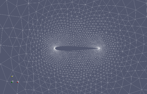
This section shows the effect of an approximate linearization on the accuracy of the sensitivity computation. The first two sets of results portray the effect of partial linear solves on the accuracy of the identity of the differentiation of the inverse matrix in the sensitivity computation shown in equation (28). The final set shows the impact of exactly linearizing the residual operator at every stage of a Runge-Kutta scheme when the gradients are only computed at the first stage and then frozen throughout the analysis. All cases were run on an unstructured triangular mesh consisting of 4212 elements shown in Figure (1), in flow with , with 2 Hickes-Henne bump functions HicksHenneDesign used as design variables to perturb the airfoil surface.
7.1 Results for an Exact Jacobian Augmented with a Mass Matrix
Here we look at the impact of inexact linearization for an exact Newton algorithm, when the left hand side is the exact linearization of the residual operator augmented with a suitable mass matrix. The fixed point iteration is shown below,
| (94) |
where is computed by solving the linear system below to a linear tolerance of the user’s choice; in this work FGMRES algorithm GMRES ; PTA-iqn is used to solve said linear system, except for the cases where we show duality, where we use Gauss-Seidel sweeps as they are right-hand-side independent.
| (95) |
where R is the residual operator of the discretization and is a left hand side matrix that determines the solver. As this is an exact Newton algorithm, is the Jacobian of the spatial discretization augmented with a suitable mass matrix, shown below and defined in the background section, given by
| (96) |
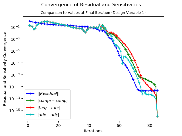
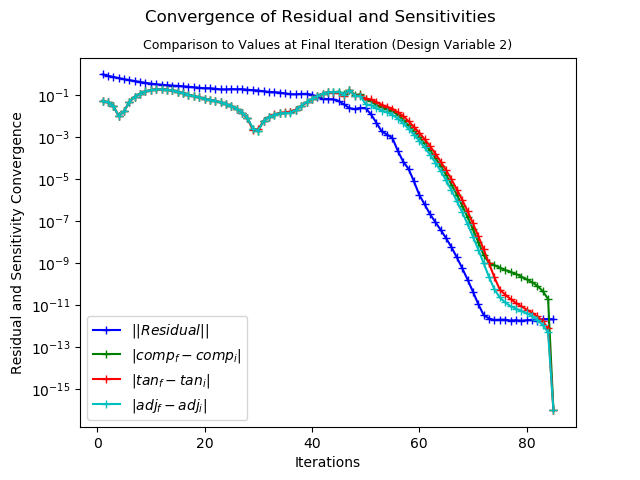
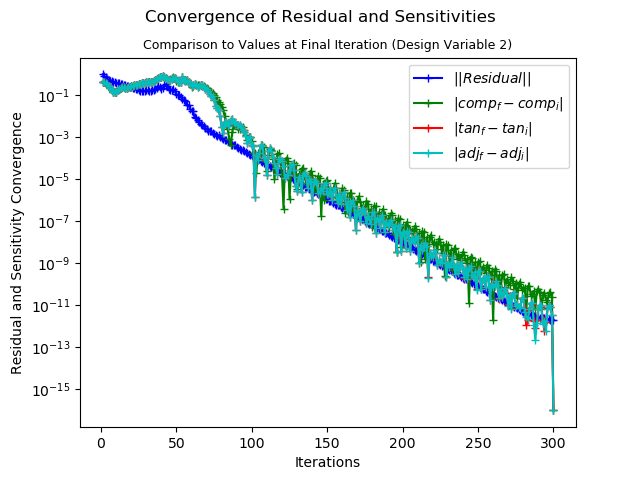
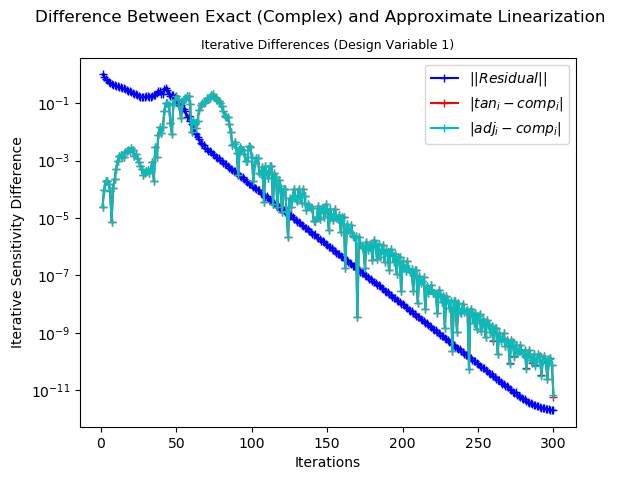
We can see in Figure (2) that for the linear tolerance the complex, tangent, and adjoint sensitivities, converge to their final values at the same rate as the analysis problem itself, which is expected based on the formulation. We can then see in Figure (3), which depicts the difference between the complex and tangent sensitivities over the iteration history of the analysis solution process, that the maximum difference is of the order of the linear tolerance of the linear system. Furthermore, as the analysis problem converges, so do the complex, tangent, and adjoint sensitivities to each other despite the inexact differentiation. We can see that at full convergence of the analysis problem, the adjoint, tangent and complex-step sensitivities correspond to each other to a high degree of precision and these would also correspond to the steady-state tangent and adjoint computed sensitivities linearized about the converged analysis state.
2
2
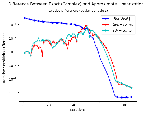
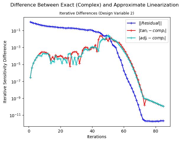
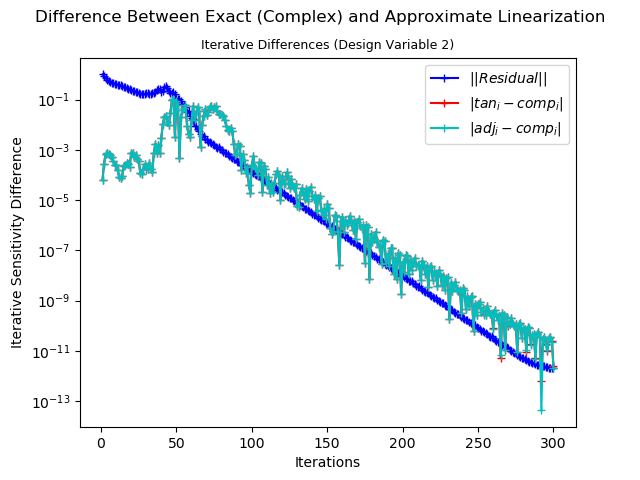
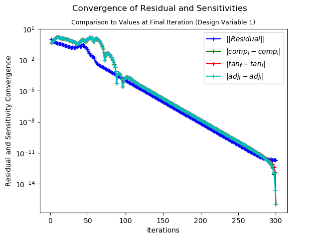
Figure (4) contains the same information as Figure (2), and Figure (3) is the sister plot of Figure (5) but the two later plots show results with a tighter linear system tolerance of . We can see that as before the maximum iterative difference is again on the order of the linear system tolerance, and that as the analysis problem converges so do the adjoint, tangent, and complex sensitivities to each other, down to nearly machine precision.
2
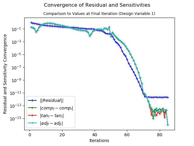
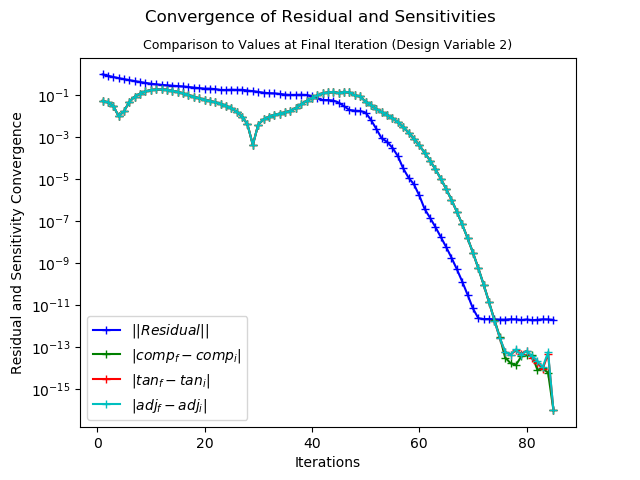
2
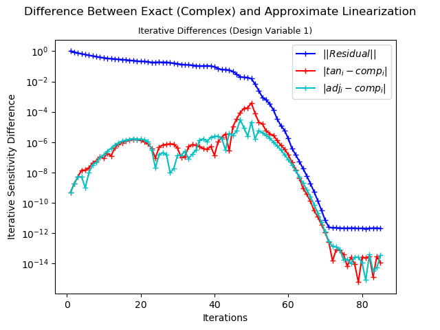
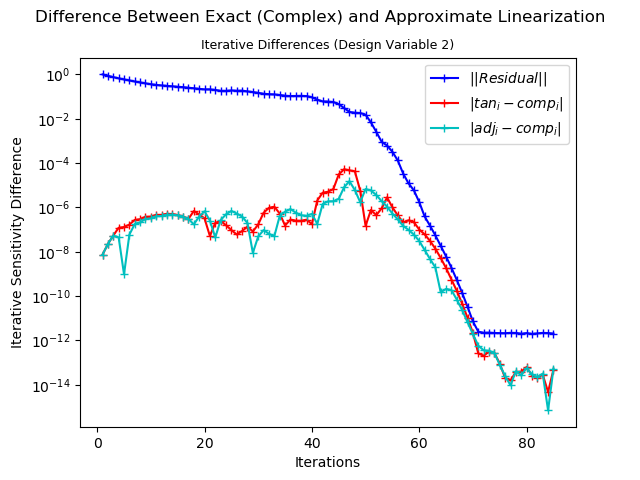
One thing to note is that while the adjoint and tangent linearizations have very similar convergence behavior, they are not identical. That is because these simulations use a specified linear tolerance to terminate the linear solver, and the number of steps is not identical between the tangent and adjoint linearizations. The goal of this investigation is to show similar behavior despite the loss of strict duality as identical behavior has already been shown for cases when strict duality is maintained PTA-devel .
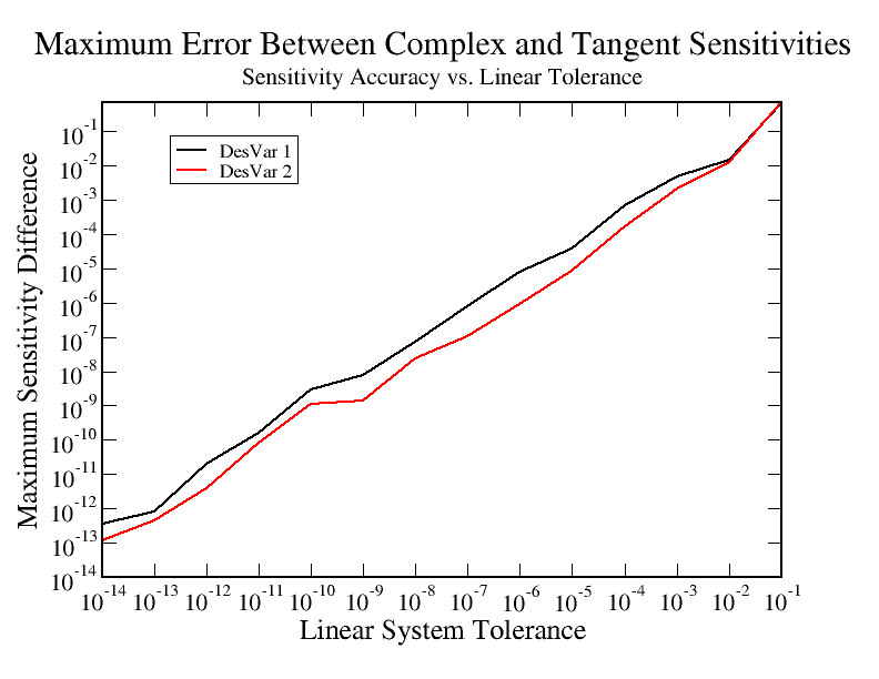
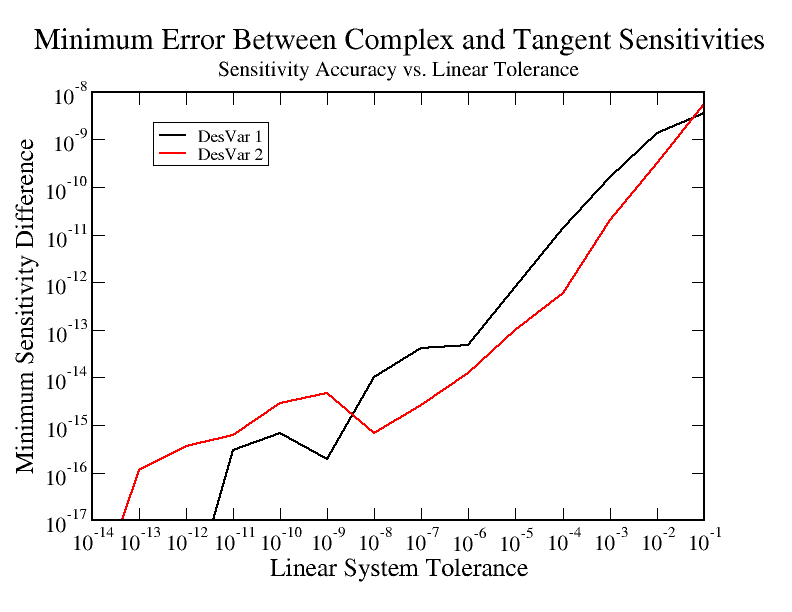
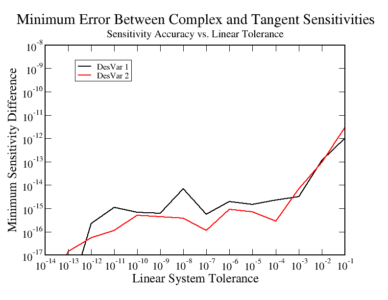
Having seen the impact of the tighter linear system tolerance on the maximum iterative difference between the tangent and complex-step finite-difference computed sensitivities, we simulate the analysis problem with linear tolerances at every order from to , and plot the maximum iterative difference in Figure (6). The maximum iterative difference is directly related to the linear system tolerance. This allows for good estimates of the maximum iterative error as a function of the linear system tolerance. The minimum iterative difference shows similar behavior, but it is a function of the linear tolerance and the convergence of the non-linear problem.
2 .
7.2 Results for an Inexact Jacobian Augmented with a Mass Matrix
Here we show the impact of inexact linearization for an inexact-quasi-Newton algorithm, i.e. the left hand side is the first order linearization of the second order residual operator augmented with a suitable mass matrix. Similar to the previous section the nonlinear solver is defined by
| (97) |
where is computed by solving the linear system
| (98) |
to a linear tolerance of the user’s choice using the same algorithms as in the exact Newton section.
However, here is an inexact linearization; it is the Jacobian of the first order spatial discretization augmented with a diagonal term to ensure that it is diagonally dominant, shown in equation (99):
| (99) |
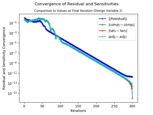
This form is used as it is representative of a typical implicit solver used in CFD problems, and the expectation is that we see similar behavior to that seen in the previous section. In this case, rather than observing quadratic convergence in both the primal and tangent/adjoint linearizations, we expect to see linear convergence in the primal problem and its linearizations. To demonstrate this we show sister plots to those of the previous section, but for the inexact Newton runs. Figures (7, 8) show the behavior for a linear tolerance of and Figures (9, 10) show the behavior for a tolerance of . These are the same tolerances we portrayed in the previous section, and we can see the same expected convergence of the inexactly linearized tangent and adjoint computed sensitivities to the complex linearization. We can see again, and as hypothesized by the error bounds in this work, that the maximum iterative difference is again on the order of the linear system tolerance, and that as the analysis converges so do the adjoint, tangent, and complex sensitivities to each other, down to nearly machine precision.
2
2
2
2
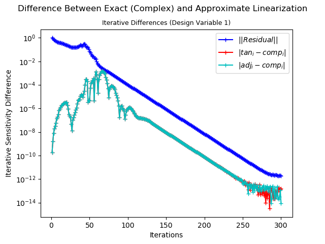
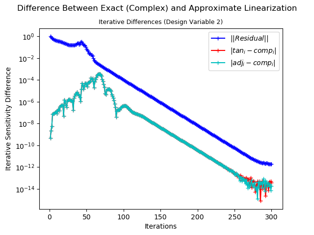
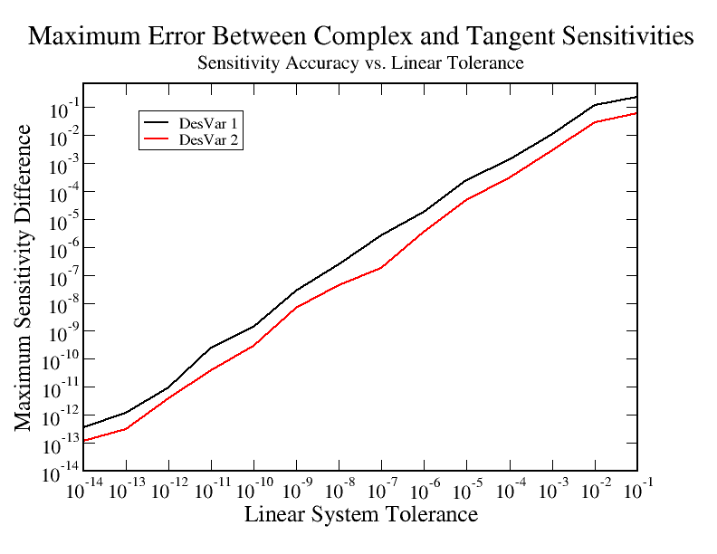
Having seen the impact of the tighter linear system tolerance on the maximum iterative difference between the adjoint, tangent, and complex sensitivities in Figure (6), and seeing the expected behavior as shown in the theoretical error bound in Proposition (1) and the previous section, we then simulate to check the impact of linear tolerances from to . When we plot the maximum iterative difference in Figure (11) we see the expected behavior over that parameter sweep. This confirms the theoretical bound applies to a more general solver, one in which the left hand side is not an exact linearization of the right hand side. Again, we see similar behavior between the tangent and adjoint linearizations but not identical as we have lost strict duality as we have not maintained the same number of linear iterations in the adjoint, tangent, and primal problems.
2 .
7.3 Results for Inexactly Linearized Explicit Runge-Kutta Solver
To check the effect of inexact linearization of the fixed point iteration for an explicit Runge-Kutta solver, we calculate the flow gradients for the base stage, and then hold them frozen through the fixed point iteration that solves the primal problem. For the linearization of the fixed point iteration we still update the gradients at each step and compute the Jacobian of the flow accordingly. To clarify the implementation we refer to the spatial residual as a summation over the edges or faces that construct the control volume, where the summation depends on the reconstructed states () given by
| (100) |
Where and are defined as the inviscid flux normal to the face and the face unit normal. The states and are reconstructed from the respective cell centers to the midpoint of the face separating cells j and k, and it becomes clearer how this inaccuracy is introduced. The reconstruction is implemented as
| (101) | ||||
where are the cell center values at cells and respectively, and are the vectors from the respective element centers to the midpoint of the face separating the elements. The explicit Runge-Kutta solver is expressed below, iterating through pseudo time and through stages 1 to 5:
| (102) |
with the end of the sub-stage time-stepping being governed as follows:
| (103) |
The primal problem fixed-point iteration uses the flow gradients from the base stage, i.e.:
| (104) | ||||
but the inexact tangent and adjoint linearizations recompute the gradients at each stage as shown below.
| (105) | ||||
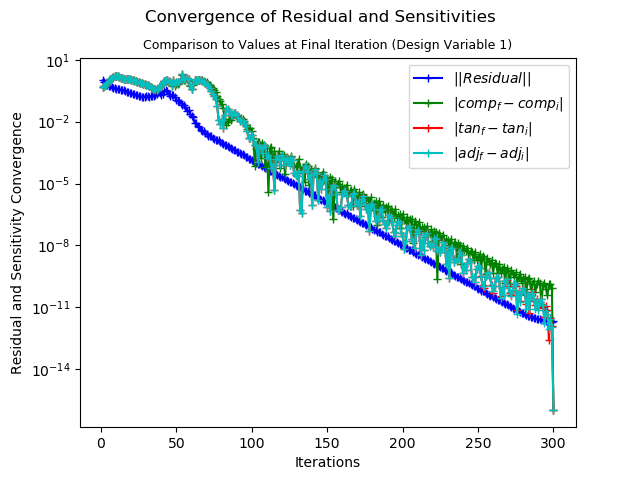
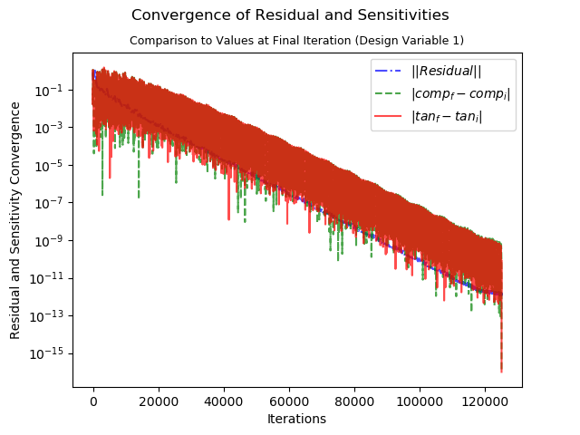
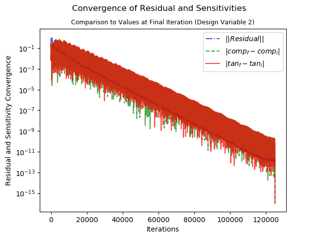
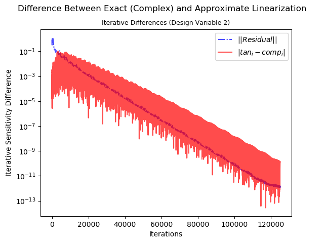
This allows us to look at the Runge-Kutta scheme as some A operator depending on the flow state and design variables that multiplies the 0-stage residual to get , where the linearization of A is inexact due to the inconsistent handling of the gradients. When we look at the convergence of the flow sensitivities to their respective final values as we did in the two previous sections, Figure (12) shows them converging to their respective final values as the primal problem converges.
2
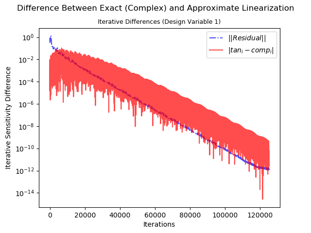
Looking at the difference between the complex (exact) linearization and the approximate tangent linearization portrayed in Figure (13) shows the expected behavior. We see the error due to the inexact linearization of the Runge-Kutta scheme goes away at the rate of the primal problem convergence as shown in the proof section and the previous results. Due to the high number of iterations for the explicit Runge-Kutta solver a visualization of the comparison between the adjoint sensitivities and the complex-step finite difference computed ones is not possible, as this would be on the order of the number of iterations squared, but the expected behvaior is shown for the tangent as discussed previously, and the adjoint is the dual and has similar convergence properties.
2
8 Conclusion and Future Work
The motivation for this work was to better understand the successful usage of the pseudo-time accurate adjoint algorithm when applied to sensitivity computation and optimization for nonconvergent simulations PTA-iqn ; to that end we sought to better understand the error introduced to the sensitivity computation by using inexact linearizations of fixed point iterations. In this paper, we showed that the error between the approximate linearization and the complex (exact) linearization of a fixed point iteration is a function of both the satisfaction of the discretized PDE denoted by the residual norm and the accuracy of the approximation of the fixed point iteration itself. We proved that in the limit of machine zero convergence of the nonlinear problem this approximation error vanishes. Furthermore, we have shown that we can obtain reasonable sensitivities for optimization without exact linearization of the fixed point iteration or full convergence of the non-linear problem, such that the error in the sensitivities depends on level of convergence in the non-linear and linear problems combined. This allows a user to select for the level of accuracy they desire in the sensitivities used for the optimization process. Finally, we demonstrated this behavior in a CFD code for an exact quasi-Newton solver, an inexact quasi-Newton solver and a five stage low-storage explicit Runge-Kutta solver. These proofs and results can also be useful in the analysis and implementation of automatic differentiation software, where the topic of error due to linearization of inexact linear solution processes is under investigation. Further future work in this area will relate to investigating other less accurate approximate linearizations and their use in optimization as well as using approximate linearizations in the aformentioned ”piggy-back” iterations of the one-shot adjoint, where the authors believe similar proofs on error convergence can be shown and used to great effect. An additional application is that, having shown the convergence of the approximate linearizations parallels that of the non-linear problem, we can pair these approximate linearizations with work on design under inexact PDE constraints SKN to get a more efficient design process for well-converging simulations.
9 Acknowledgments
This work was supported in part by NASA Grant NNX16AT23H and the NASA Graduate Aeronautics Scholars Program. Computing time was provided by ARCC on the Teton supercomputer.
10 Conflict of Interest
The authors declare that they have no conflict of interest.
References
- (1) Ahrabi, B.R., Mavriplis, D.J.: An implicit block ilu smoother for preconditioning of newton–krylov solvers with application in high-order stabilized finite-element methods. Computer Methods in Applied Mechanics and Engineering 358, 112,637 (2020). DOI https://doi.org/10.1016/j.cma.2019.112637. URL http://www.sciencedirect.com/science/article/pii/S0045782519305213
- (2) Akbarzadeh, S., Huckelheim, J., Muller, J.D.: Consistent treatment of incompletely converged iterative linear solvers in reverse-mode algorithmic differentiation. Computational Optimization and Applications DOI 10.1007/s10589-020-00214-x. URL https://link.springer.com/article/10.1007/s10589-020-00214-x
- (3) Brown, D.A., Nadarajah, S.: An adaptive constraint tolerance method for optimization algorithms based on the discrete adjoint method DOI 10.2514/6.2018-0414. URL https://arc.aiaa.org/doi/abs/10.2514/6.2018-0414. 2018 AIAA/ASCE/AHS/ASC Structures, Structural Dynamics, and Materials Conference, AIAA SciTech Forum, AIAA Paper 2018-0414, Kissimmee, Florida, 01/2018, https://doi.org/10.2514/6.2018-0414
- (4) Gill, P.E., Murray, W., Saunders, M.A.: Snopt: An sqp algorithm for large-scale constrained optimization. SIAM review 47(1), 99–131 (2005)
- (5) Griewank, A., Ponomarenko, A.: Time-lag in derivative convergence for fixed point iterations. In: Proceedings of CARI’04, 7th African Conference on Research in Computer Science, pp. 295–304 (2004)
- (6) Gunther, S.: Simultaneous optimization with unsteady partial differential equations. Doctoral thesis, RWTH Aachen (2017). URL http://publications.rwth-aachen.de/record/696346/files/696346.pdf
- (7) Günther, S., Gauger, N.R., Wang, Q.: Simultaneous single-step one-shot optimization with unsteady pdes. J. Comput. Appl. Math. 294, 12–22 (2016)
- (8) Hicks, R.M., Henne, P.A.: Wing design by numerical optimization. Journal of Aircraft 15(7), 407–412 (1978). DOI 10.2514/3.58379. URL https://doi.org/10.2514/3.58379
- (9) Krakos, J.A., Darmofal, D.L.: Effect of small-scale output unsteadiness on adjoint-based sensitivity. AIAA Journal 48(11), 2611–2623 (2010). DOI 10.2514/1.J050412. URL https://doi.org/10.2514/1.J050412
- (10) Krakos, J.A., Wang, Q., Hall, S.R., Darmofal, D.L.: Sensitivity analysis of limit cycle oscillations. Journal of Computational Physics 231(8), 3228 – 3245 (2012). DOI https://doi.org/10.1016/j.jcp.2012.01.001. URL http://www.sciencedirect.com/science/article/pii/S0021999112000071
- (11) van Leer, B.: Flux-vector splitting for the euler equations. In: E. Krause (ed.) Eighth International Conference on Numerical Methods in Fluid Dynamics, pp. 507–512. Springer Berlin Heidelberg, Berlin, Heidelberg (1982)
- (12) LeVeque, R.J.: Numerical Methods for Conservation Laws, vol. 3. Springer (1992)
- (13) Mavriplis, D.: Revisiting the least-squares procedure for gradient reconstruction on unstructured meshes DOI 10.2514/6.2003-3986. URL https://arc.aiaa.org/doi/abs/10.2514/6.2003-3986. 16th AIAA Computational Fluid Dynamics Conference, Fluid Dynamics and Co-located Conferences, AIAA Paper 2003-3986, Orlando, Florida, 06/2003. https://doi.org/10.2514/6.2003-3986
- (14) Mavriplis, D.: A residual smoothing strategy for accelerating newton method continuation. arXiv preprint arXiv:1805.03756 (2018)
- (15) Mavriplis, D.J.: Vki lecture series: 38th advanced computational fluid dynamics. adjoint methods and their application in cfd, time dependent adjoint methods for single and multi-disciplinary problems (2015)
- (16) Nadarajah, S.K.: The Discrete Adjoint Approach to Aerodynamic Shape Optimization, Ph.D. Dissertation. Department of Aeronautics and Astronautics, Stanford University, USA (2003)
- (17) Nemec, M., Aftosmis, M.J.: Toward automatic verification of goal-oriented flow simulations. Tech. Rep. Tech. Rep. TM-2014-218386, NASA Ames Research Center (2014). URL https://ntrs.nasa.gov/search.jsp?R=20150000864
- (18) Padway, E., Mavriplis, D.J.: Advances in the pseudo-time accurate formulation of the adjoint and tangent systems for sensitivity computation and design DOI doi:10.2514/6.2020-3136. URL https://arc.aiaa.org/doi/abs/10.2514/6.2020-3136. 59th AIAA Aerospace Sciences Meeting, AIAA Paper 2020-3136, Virtual Event, June 2020. https://doi.org/10.2514/6.2020-3136
- (19) Padway, E., Mavriplis, D.J.: Application of the pseudo-time accurate formulation of the adjoint to output-based adaptive mesh refinement DOI doi:10.2514/6.2021-1326. URL https://arc.aiaa.org/doi/abs/10.2514/6.2021-1326. 59th AIAA Aerospace Sciences Meeting, AIAA Paper 2021-1326, Virtual Event, January 2021. https://doi.org/10.2514/6.2021-1326
- (20) Padway, E., Mavriplis, D.J.: Toward a pseudo-time accurate formulation of the adjoint and tangent systems DOI 10.2514/6.2019-0699. URL https://arc.aiaa.org/doi/abs/10.2514/6.2019-0699. 57th AIAA Aerospace Sciences Meeting, AIAA Paper 2019-0699, San Diego CA, January 2019. https://doi.org/10.2514/6.2019-0699
- (21) Roe, P.: Approximate riemann solvers, parameter vectors, and difference schemes. Journal of Computational Physics 135(2), 250 – 258 (1997). DOI https://doi.org/10.1006/jcph.1997.5705. URL http://www.sciencedirect.com/science/article/pii/S0021999197957053
- (22) Saad, Y.: Iterative methods for sparse linear systems, vol. 82. Society for Industrial and Applied Mathematics (2003). DOI 10.1137/1.9780898718003
- (23) Sagebaum, M.: Advanced techniques for the semi automatic transition from simulation to design software. Doctoral thesis, Technische Universität Kaiserslautern (2018). URL http://nbn-resolving.de/urn:nbn:de:hbz:386-kluedo-53891
- (24) Venditti, D.A., Darmofal, D.L.: Anisotropic grid adaptation for functional outputs: Application to two-dimensional viscous flows. J. Comput. Phys. 187(1), 22–46 (2003). DOI 10.1016/S0021-9991(03)00074-3. URL https://doi.org/10.1016/S0021-9991(03)00074-3