Uncertainty-aware Joint Salient Object and Camouflaged Object Detection

Abstract

Visual salient object detection (SOD) aims at finding the salient object(s) that attract human attention, while camouflaged object detection (COD) on the contrary intends to discover the camouflaged object(s) that hidden in the surrounding. In this paper, we propose a paradigm of leveraging the contradictory information to enhance the detection ability of both salient object detection and camouflaged object detection. We start by exploiting the easy positive samples in the COD dataset to serve as hard positive samples in the SOD task to improve the robustness of the SOD model. Then, we introduce a “similarity measure” module to explicitly model the contradicting attributes of these two tasks. Furthermore, considering the uncertainty of labeling in both tasks’ datasets, we propose an adversarial learning network to achieve both higher order similarity measure and network confidence estimation. Experimental results on benchmark datasets demonstrate that our solution leads to state-of-the-art (SOTA) performance for both tasks.

1 Introduction

Visual salient object detection (SOD) aims to localize the most salient region(s) of the images that attract human attention. To be qualified as a “salient” object, one should have high contrast compared with its global and local context. The camouflaged objects oppositely usually share similar structure or texture information with the environment, which try hard to fade themselves into the local context. In this way, the SOD models [48, 46, 42, 38] are designed based on both global contrast and local contrast, while the COD models [11, 26, 35, 52, 34] usually avoid searching the camouflaged objects in those salient regions. We notice that a higher level of saliency indicates a lower level of camouflage and vice versa as shown in Fig. 1. This observation shows that the salient objects and camouflaged objects are two contradicting categories of objects. However, there still exist objects that are both salient and camouflaged, the polar bear in the middle of Fig. 1, which indicates that these two tasks are partially positively related at the dataset level.

Existing SOD models [48, 47, 59, 46, 38] mainly focus on two directions: 1) building effective saliency network [47, 59] for accurate saliency detection with pixel-wise accuracy constraint; and 2) designing appropriate loss functions [46, 38] to achieve structure-preserving saliency detection. The former digs into network structure, while the latter cares more about network loss function. We argue that an effective training dataset can lead to more performance gain in addition to network structure design or loss function, it’s the training data that is regressed.

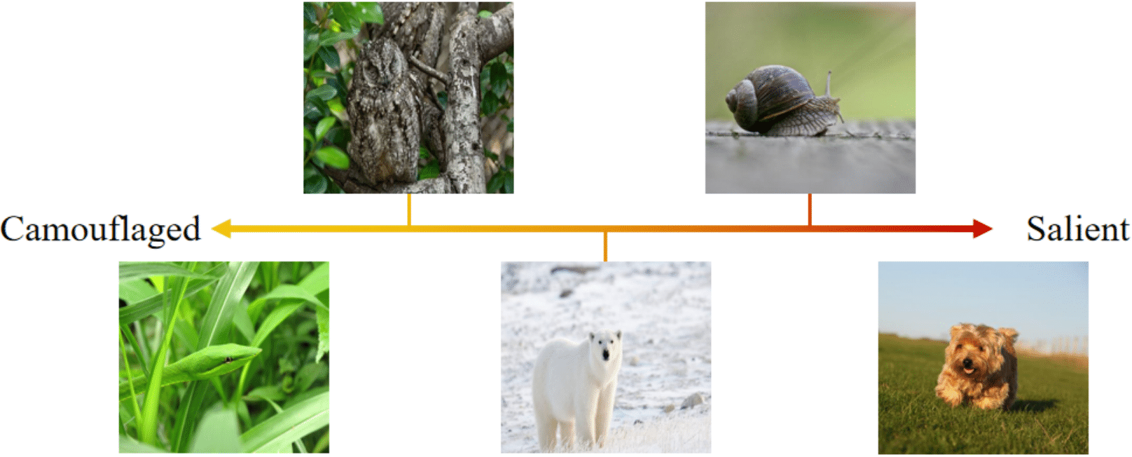
Figure 1: Illustration of the transition from camouflaged objects to salient objects, where the image in the middle could belong to both camouflaged object dataset and salient object dataset.

One typical solution to explore the training dataset is data augmentation, which usually involves linear or non-linear transformation of the dataset. We find that, although performance improvement can be obtained with some basic data augmentation, image flipping, rotation, cropping, and , none of these methods are specially designed for saliency detection. As a context-based task, a more effective data augmentation technique should be context-aware. For SOD, the salient objects are those that can be easily detected, or the high-contrast objects as shown in Fig. 1. We intend to augment the dataset to include lower contrast samples. Considering the partial positively related attribute of SOD and COD at dataset level, we intend to design a joint learning framework to learn both tasks and select easy samples from COD (the polar bear) as hard samples for SOD, achieving contrast-level data augmentation.

Joint training is mostly designed for positively related tasks [43, 14, 51]. In contrary, we propose to integrate two contradicting tasks (SOD and COD) into one network with a “Similarity measure” module as shown in Fig. 2. The basic assumption of our similarity measure module is that the activated regions of the same image for the two tasks should be different, leading to latent features apart from each other. To this end, we introduce the third dataset, PASCAL VOC 2007 images [7] in particular, to our framework serving as the connection modeling dataset. The goal of these extra images is to achieve similarity measures and force the two tasks to focus on different regions of the image.

Moreover, as shown in Fig. 1, the salient object is salient in both local and global contexts, while the camouflaged object is hiding in its local context. Due to the high contrast, the local context of the salient objects is easier to model than that of the camouflaged objects, as there exists no clear boundary between camouflaged objects and their surrounding. By jointly training a salient object detection network and camouflaged object detection network, the salient object branch can learn precise local context information for accurate camouflaged object detection.

Lastly, we observe two types of uncertainty while labeling the dataset for each task. For salient object detection, the subjective nature of saliency [55, 54, 53] leads to ambiguity of prediction, as shown in Fig. 5(a). For camouflaged object detection, the uncertainty comes from the difficulty in fully annotating the camouflaged objects as they usually share similar color or texture with the environment, as shown in Fig. 5(c). We then introduce adversarial training to explicitly model the confidence of network predictions, and estimate model uncertainty for both tasks.

We summarize our main contributions as: 1) We introduce the first joint salient object detection and camouflaged object detection network within an adversarial learning framework to explicitly model prediction uncertainty of each task. 2) We design the similarity measure module to explicitly model the “contradicting” attributes of the two tasks. 3) We present a data interaction strategy and treat easy samples from camouflage dataset as hard samples for saliency detection, achieving a robust saliency model.

2 Related Work

Salient Object Detection Models Existing deep saliency detection models [47, 48, 42, 29, 46, 12, 38] are mainly designed to achieve structure-preserving saliency predictions. [38, 48] introduced auxiliary edge detection branch to produce a saliency map with precise structure information. Wei et al.[46] presented structure-aware loss function to penalize prediction along object edges. Wu et al.[47] designed a cascade partial decoder to achieve accurate saliency detection with finer detailed information. Feng et al.[12] proposed a boundary-aware mechanism to improve the accuracy of network prediction on the boundary. There also exist salient object detection models that benefit from data of other sources. [45, 24] integrated fixation prediction and salient object detection in a unified framework to explore the connections of the two related tasks. Zeng et al.[51] presented to jointly learn a weakly supervised semantic segmentation and fully supervised salient object detection model to benefit from both tasks.

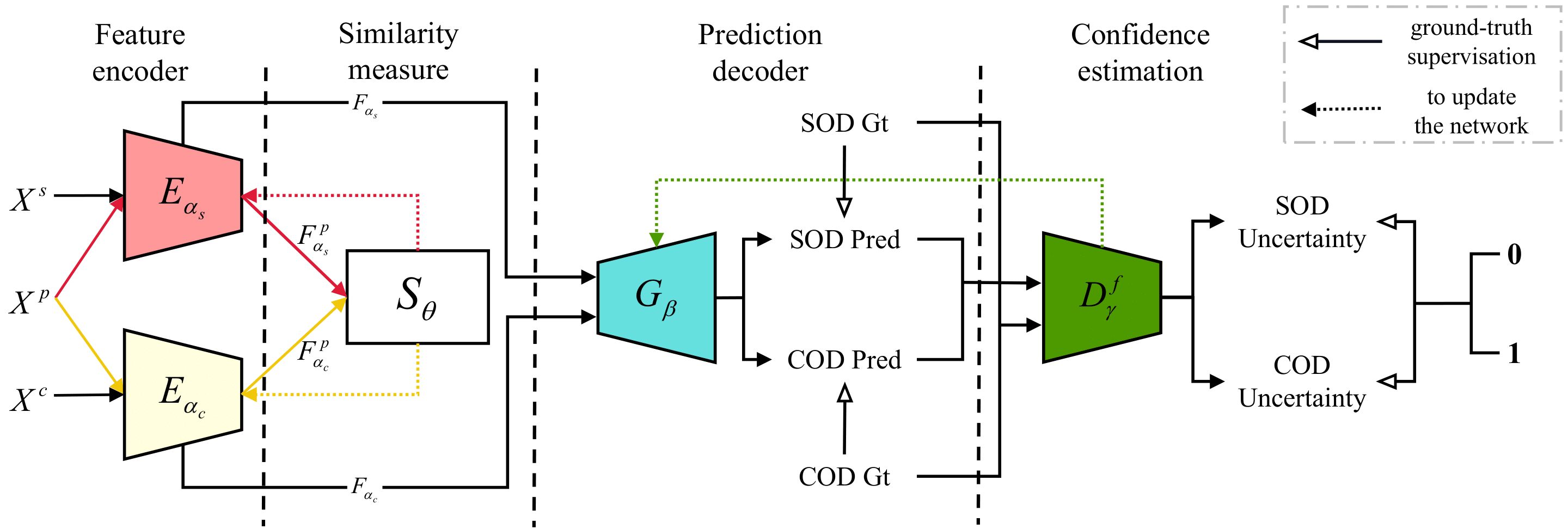
Figure 2: Overview of the proposed network. The “Feature encoder” module extracts task-specific features for image $X^{s}$ and $X^{c}$ from SOD and COD dataset respectively. And for the connection modeling data $X^{p}$, we introduce “Similarity measure” to explicitly model the contradicting attribute of SOD and COD. The shared “Prediction decoder” module is used to generate predictions for both tasks. The shared “Confidence estimation” module is a fully convolutional discriminator, which estimates the pixel-wise confidence of network prediction.

Camouflaged Object Detection Models Camouflage models are designed to discover the camouflaged object(s) hidden in the surrounding. Different from salient objects, which are those attracting human attention, camouflaged objects are those trying to decrease the conspicuousness. The concept of camouflage is usually associated with context [1, 2, 5]. Cuthill et al.[6] presented that an effective camouflage includes two mechanisms: the background pattern matching, where the color is similar to the environment, and the disruptive coloration, which usually involves bright colors along edge, and makes the boundary between camouflaged objects and the background unnoticeable. Bhajantri et al.[3] utilized co-occurrence matrix to detect defective. Pike et al.[37] combined several salient visual features to quantify camouflage, which could simulate the visual mechanism of a predator. In the field of deep learning, Fan et al.[11] proposed the first publicly available camouflage deep network with the largest camouflaged object training set.

Multi-task Learning The basic assumption behind multi-task learning is that there exists shared information among different tasks. In this way, multi-task learning is widely used to extract complementary information about positively related tasks. Kalogeiton et al.[22] jointly detected objects and actions in a video scene. Zhen et al.[58] designed a joint semantic segmentation and boundary detection framework by iteratively fusing feature maps generated for each task with pyramid context module. In order to solve the problem of insufficient supervision in semantic alignment and object landmark detection, Jeon et al.[19] designed a joint loss function to impose constraints between tasks, and only reliable matched pairs were used to improve the model robustness with weak supervision. Joung et al.[21] solved the problem of object viewpoint changes in 3D object detection and viewpoint estimation with a cylindrical convolutional network, which obtains view-specific features with structural information at each viewpoint for both two tasks. Luo et al.[32] presented a multitask framework for referring expression comprehension and segmentation.

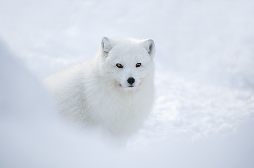
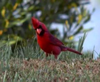
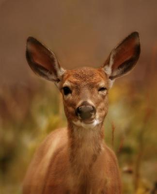
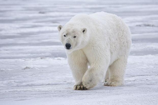
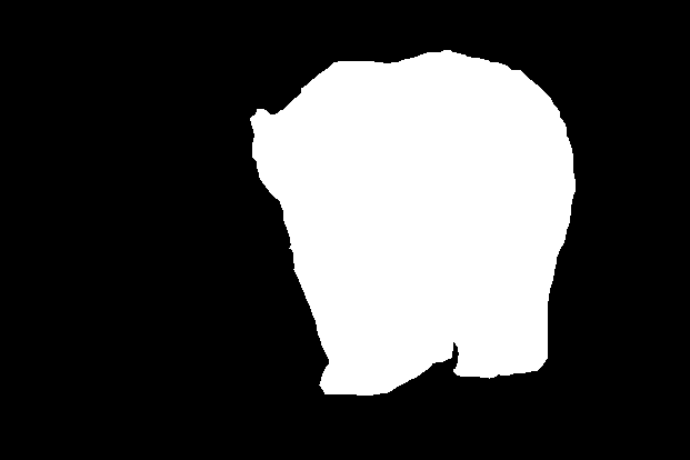
Figure 3: Selected easy samples from the COD training dataset.

Adversarial Learning Adversarial learning is an effective solution to improve the robustness of the deep neural network. In fully supervised models, adversarial learning can measure higher-order inconsistencies between labels and predictions [25]. Specifically, Li et al.[28] introduced generic noise to destroy adversarial perturbation of the input image for salient object detection. [31, 41] built the Generative Adversarial Network (GAN) [16] based saliency detection network, where the fully connected discriminator was used to distinguish the real saliency map (ground truth) from the fake saliency map (prediction). Similarly, Jiang et al.[20] designed a GAN based framework for RGB-D saliency detection to solve the cross-modality detection problem. In the case of insufficient annotations, adversarial learning can serve as guidance to select confident samples or generate new samples. Souly et al.[40] used adversarial learning to generate fake images with image-level labels and noise, which in turn can make the real samples gathering in feature space and improve accuracy for weakly supervised semantic segmentation. [18, 36] treated adversarial learning as a confidence measure to obtain the trustworthy regions of semantic segmentation predictions of unlabeled data for semi-supervised learning.

Different from existing multi-task learning frameworks that mainly benefit from positively related tasks, we instead build the connections of two contradicting tasks within a joint learning framework by explicitly modeling the contradicting attributes with a similarity measure module.

3 Our Method

We design an uncertainty-aware joint learning framework as shown in Fig. 2 to learn SOD and COD in a unified framework. Firstly, as a data augmentation technique, we select a group of easy samples from the COD training dataset to achieve robust SOD. Then, we present the “Similarity measure” module to explicitly model the “contradicting” attributes of the two tasks. Lastly, we introduce our uncertainty-aware adversarial training network to produce interpretable predictions during testing, and achieve higher-order similarity measure during training.

3.1 Data interaction as data augmentation

As shown in Fig. 1, there exist samples in the COD dataset that are both salient and camouflaged. We argue that those samples can be treated as hard samples for salient object detection to achieve robust learning. To select those samples from the COD dataset, we resort to Mean Absolute Error (MAE), and select samples in COD dataset [11] which achieve the smallest MAE by testing it using a trained SOD model [48]. Specifically, for camouflaged object detection training dataset $D_{c}=\{X_{i}^{c},Y_{i}^{c}\}_{i=1}^{N_{c}}$, where $i$ indexes the images, and $N_{c}$ is the size of camouflaged object detection training set. We defined the trained SOD model as $M_{\theta_{s}}$. Then we obtain saliency prediction of the images in $D_{c}$ as $P^{c}_{s}=M_{\theta_{s}}(X^{c})=\{p^{c}_{i}\}_{i=1}^{N_{c}}$, where $p_{i}^{c}$ is the saliency prediction in COD training dataset. We assume that easy samples for COD can be treated as hard samples for SOD as shown in Fig. 1. Then we select $M=400$ samples $D_{c}^{M}$ of the smallest MAE in $D_{c}$, and replace it with $M=400$ randomly selected samples in our SOD training dataset [44] as a data augmentation technique. We show the selected samples in Fig. 3, which clearly illustrates the partially positive connection of the two tasks at the dataset level.

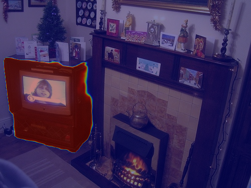
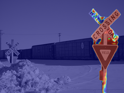
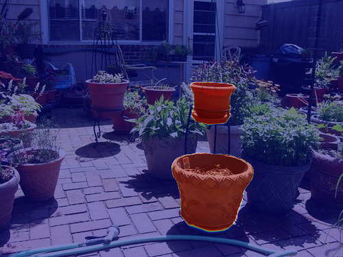
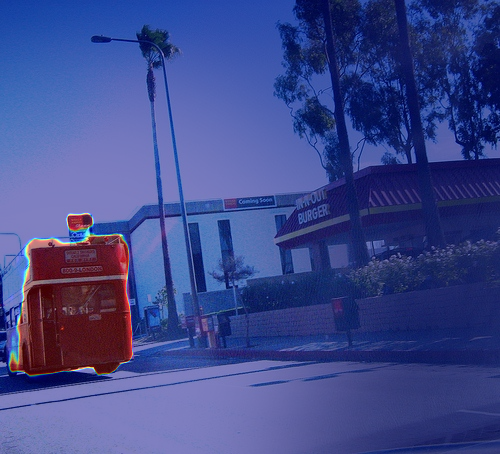
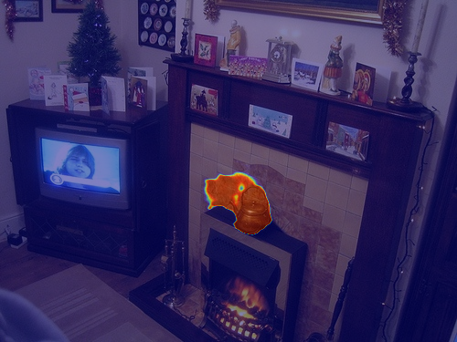
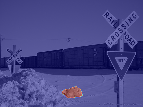
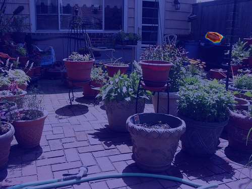
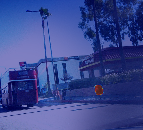
Figure 4: Detected region from the saliency encoder branch (first row) and the camouflage encoder branch (second row).

3.2 Contradicting modeling

Similar as above, let’s define our camouflaged object detection training dataset as $D_{c}=\{X_{i}^{c},Y_{i}^{c}\}_{i=1}^{N_{c}}$ and augmented salient object detection training dataset as $D_{s}=\{X_{i}^{s},Y_{i}^{s}\}_{i=1}^{N_{s}}$, where $i$ indexes images, $X$ and $Y$ are the image and ground truth pair, $N_{c}$ and $N_{s}$ are size of the camouflage training set and saliency training set respectively. Based on the “contradicting” attribute of SOD and COD, we design a “Similarity measure” module in Fig. 2 to explicitly model the connection of the two tasks.

Specifically, we introduce another set of images from PASCAL VOC 2007 dataset [7] as “connection modeling” dataset $D_{p}=\{X_{i}^{p}\}_{i=1}^{N_{p}}$, from which we extract the camouflaged feature and the salient feature. With the three datasets (COD dataset $D_{c}$, augmented SOD dataset $D_{s}$ and connection modeling dataset $D_{p}$), our contradicting modeling framework uses the “Feature encoder” module to extract both camouflage feature and saliency feature, and then use the “Similarity measure” module to model connection of the two tasks with the connection modeling dataset.

Feature Encoder
We design both the saliency encoder $E_{\alpha_{s}}$ and camouflage encoder $E_{\alpha_{c}}$ network with the same backbone network, the ResNet50 [17], where $\alpha_{s}$ and $\alpha_{c}$ are network parameter sets of each of them respectively. Initially, the ResNet50 backbone network has four groups of convolutional layers of channel size 256, 512, 1024 and 2048 respectively. We then define the output features of both encoders as $F_{\alpha_{s}}=\{f^{s}_{1},f^{s}_{2},f^{s}_{3},f^{s}_{4}\}$ and $F_{\alpha_{c}}=\{f^{c}_{1},f^{c}_{2},f^{c}_{3},f^{c}_{4}\}$, where $f_{k},k=1,...,4$ is feature map of the $k$-th group.

Similarity Measure
Different from the feature encoder module, which takes images from $D_{c}$ and $D_{s}$ as input to produce task-specific feature maps, the similarity measure module $S_{\theta}$ takes the connection modeling data $D_{p}$ as input to model the connection of SOD and COD, where $\theta$ is parameter set of the similarity measure module. Given the trained saliency encoder $E_{\alpha_{s}}$ and camouflage encoder $E_{\alpha_{c}}$, the saliency feature and camouflage feature of images $X^{p}$ are $F^{p}_{\alpha_{s}}=\{f^{p}_{s1},f^{p}_{s2},f^{p}_{s3},f^{p}_{s4}\}$ and $F^{p}_{\alpha_{c}}=\{f^{p}_{c1},f^{p}_{c2},f^{p}_{c3},f^{p}_{c4}\}$ respectively. We then concatenate each of above two features channel-wise and feed them to the same fully connected layer to obtain the latent saliency feature and latent camouflage feature of $X^{p}$ as $f^{sp}=S_{\theta}(F^{p}_{\alpha_{s}})$ and $f^{cp}=S_{\theta}(F^{p}_{\alpha_{c}})$ respectively. Empirically, we set the dimension of the latent space as $K=700$. For the same image in $D_{p}$, we assume that the SOD network and COD network should focus on different regions, leading to different feature representation. Then, we choose the cosine similarity to measure the difference between the saliency feature and the camouflage feature in latent space, and define the latent space loss as:

$$\mathcal{L}_{latent}=cos(f^{sp},f^{cp})=\frac{f^{sp}\cdot f^{cp}}{\left\|f^{sp}\right\|\times\left\|f^{cp}\right\|}.$$ (1)

In Fig. 4, we show the activation region (the processed predictions) of the same image from both the saliency encoder (first row) and camouflage encoder (second row). Specifically, given same image $X^{p}$, we compute it’s camouflage map and saliency map, and highlight the detected foreground region in red. Fig. 4 shows that the two encoders focus on different regions of the image, where the saliency encoder pays more attention to the region that stand out from the context, and the camouflage encoder focuses more on the hidden object with similar color or structure as the background, which is consistent with our assumption that these two tasks are contradicting with each other in general.

3.3 Uncertainty-aware adversarial learning

As shown in Fig. 5, for the SOD dataset, the uncertainty comes from the ambiguity of saliency ((a) (b)), and for the COD dataset, the uncertainty results from the difficulty of annotation ((c) (d)). the ball in the orange rectangle (a) can be defined as salient, but it’s background in (b). The orange region in (c) belongs to the camouflaged object, while it’s too similar to the background, making it very difficult to create the accurate annotation. We then introduce an uncertainty-aware adversarial training strategy to model the task-specific uncertainty in our joint learning framework, which includes a “Prediction decoder” module to produce task-related predictions, a “Confidence estimation” module to estimate uncertainty of each prediction, and an adversarial learning strategy for robust model training.

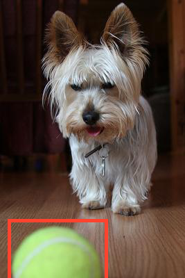
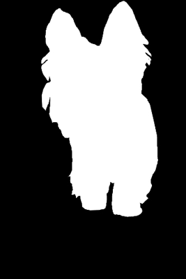
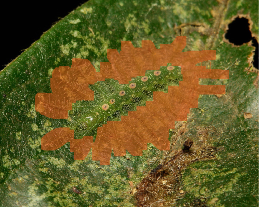
(a)	(b)	(c)	(d)

Figure 5: Uncertainty in labeling the SOD dataset ((a) and (b)) and the COD dataset ((c),(d))

Prediction decoder
As shown in Fig. 2, we design a shared decoder structure for joint SOD and COD learning. We argue that the different “Feature encoder” modules can generate task-specific features for COD images and SOD images. Then the “Prediction decoder” module aims to integrate the task-specific feature with their corresponding lower level feature to produce predictions. Specifically, given task-specific feature $F_{\alpha_{s}}=\{f^{s}_{1},f^{s}_{2},f^{s}_{3},f^{s}_{4}\}$ and $F_{\alpha_{c}}=\{f^{c}_{1},f^{c}_{2},f^{c}_{3},f^{c}_{4}\}$ from the saliency encoder and camouflage encoder respectively, the prediction decoder produces saliency map $G_{\beta}(F_{\alpha_{s}})$ and camouflage map $G_{\beta}(F_{\alpha_{c}})$, where $\beta$ is parameter set of the prediction decoder module. Specifically, we design a top-down connection network with the residual channel attention module [56] $Re$ to extract finer features. Furthermore, the dual attention module [13] $Da$ is adopted to effectively fuse higher level semantic information with the lower level structure information to obtain the initial predictions:

$$G_{init}(F_{\alpha_{s}})=C_{cla}(Re[Da(f^{s}_{4}),f^{s}_{43\_init},Da(f^{s}_{2})]),$$ (2)

$$G_{init}(F_{\alpha_{c}})=C_{cla}(Re[Da(f^{c}_{4}),f^{c}_{43\_init},Da(f^{c}_{2})]),$$ (3)

where $f_{43\_init}=conv(Re[Da(f_{4}),Da(f_{3})])$, $conv$ is the $3\times 3$ convolutional layer of output channel size $C=32$, $[.]$ is the channel-wise concatenation operation, and we upsample the features to the same spatial size before concatenation. $C_{cla}$ is the classification layer of kernel size $3\times 3$, which maps the feature map to one channel prediction for each task. Then we add a refined structure to the decoder network in order to obtain a detailed prediction $G_{\beta}(F_{\alpha_{s}})$ and $G_{\beta}(F_{\alpha_{c}})$, we use the holistic attention module [47] $Ha$ to integrate features:

$$f_{r2}=Ha(G_{init}(F_{\alpha}),f_{2}),f_{r3}=R_{3}(f_{r2}),f_{r4}=R_{4}(f_{r3}),$$ (4)

where $R_{3}$ and $R_{4}$ is the ResNet50 backbone convolutional layers of channel size 1024 and 2048 respectively. Then, we obtain the task-specific predictions $G_{\beta}(F_{\alpha_{s}})$ and $G_{\beta}(F_{\alpha_{c}})$:

$$G_{\beta}(F_{\alpha_{s}})=C_{cla}(Re[Da(f^{s}_{r4}),f^{s}_{43},f^{s}_{432},conv(f^{s}_{1})]),$$ (5)

$$G_{\beta}(F_{\alpha_{c}})=C_{cla}(Re[Da(f^{c}_{r4}),f^{c}_{43},f^{c}_{432},conv(f^{c}_{1})]),$$ (6)

where the feature $f_{43}=conv(Re[Da(f_{r4}),Da(f_{r3}])$, and the feature $f_{432}=conv(Re[Da(f_{r4}),f_{43},Da(f_{r2})])$.

Confidence Estimation
As discussed above, uncertainty exists in both SOD and COD dataset. We introduce the “Confidence estimation” module to explicitly model the confidence of network predictions. Specifically, we design a fully convolutional discriminator network to evaluate confidence of the predictions from the “Prediction decoder” module. The fully convolutional discriminator network $D^{f}_{\gamma}$ consists of five convolution layers as shown in Table 1, and produce a one-channel confidence map, where $\gamma$ is the network parameter set. Note that, we have the batch normalization and leaky relu layers after the first four convolutional layers. $D^{f}_{\gamma}$ aims to produce all-zero output with prediction $G_{\beta}(F_{\alpha_{s}})$ or $G_{\beta}(F_{\alpha_{c}})$ as input, and all-one matrix with ground truth as input.

Adversarial Learning
We introduce adversarial learning to learn both the “Prediction decoder” and the “Confidence estimation” modules.

Table 1: Network structure of the discriminator network.

Input Channel	Output Channel	kernel size	Stride	Padding
1	64	3	2	1
64	64	3	1	1
64	64	3	2	1
64	64	3	1	1
64	1	3	2	1

For the prediction decoder module, we first have the task-specific loss function to learn each task. Specifically, we adopt the structure-aware loss function [46] for both SOD and COD, and define the loss function as:

$$\mathcal{L}_{str}(Pred,Y)=\omega*\mathcal{L}_{ce}(Pred,Y)+\mathcal{L}_{iou}(Pred,Y),$$ (7)

where $\omega$ is the edge-aware weight, which is defined as $\omega=1+5*\left|(avg\_pool(Y)-Y)\right|$, $\mathcal{L}_{ce}$ is the cross-entropy loss, $\mathcal{L}_{iou}$ is the boundary-IOU loss [33], which is defined as:

$$\mathcal{L}_{iou}=1-\frac{\omega*inter+1}{\omega*union-\omega*inter+1},$$ (8)

where $inter=Pred*Y$, and $union=Pred+Y$.

And we have the structure-aware loss function for SOD and COD as:

$$\mathcal{L}_{str}^{s}=0.5*[{L}_{str}(G_{init}(F_{\alpha_{s}}),Y^{s})+{L}_{str}(G_{\beta}(F_{\alpha_{s}}),Y^{s})],$$ (9)

$$\mathcal{L}_{str}^{c}=0.5*[{L}_{str}(G_{init}(F_{\alpha_{c}}),Y^{c})+{L}_{str}(G_{\beta}(F_{\alpha_{c}}),Y^{c})].$$ (10)

To achieve adversarial learning, we have adversarial loss for both SOD and COD, which is defined as cross-entropy loss between network prediction and the pre-defined “real” indicator as:

$$\mathcal{L}_{adv}^{s}=\mathcal{L}_{ce}(D_{\gamma}^{f}(G_{\beta}(F_{\alpha_{s}})),\mathbf{1}),$$ (11)

$$\mathcal{L}_{adv}^{c}=\mathcal{L}_{ce}(D_{\gamma}^{f}(G_{\beta}(F_{\alpha_{c}})),\mathbf{1}),$$ (12)

respectvely for each task, where $\mathbf{1}$ is an all-one matrix. In this way, the discriminator takes model prediction as input, and tries to recognize it as real ground truth.

For the confidence estimation module, similar to the typical definition of discriminator in GAN [16], we want it to clearly distinguish model prediction and ground truth map. Then, the adversarial loss for the confidence estimation module of the SOD task is defined as:

$$\mathcal{L}_{dis}^{s}=\mathcal{L}_{ce}(D_{\gamma}^{f}(G_{\beta}(F_{\alpha_{s}})),\mathbf{0})+\mathcal{L}_{ce}(D_{\gamma}^{f}(Y^{s}),\mathbf{1}).$$ (13)

We then have the adversarial loss for the COD task as:

$$\mathcal{L}_{dis}^{c}=\mathcal{L}_{ce}(D_{\gamma}^{f}(G_{\beta}(F_{\alpha_{c}})),\mathbf{0})+\mathcal{L}_{ce}(D_{\gamma}^{f}(Y^{c}),\mathbf{1}).$$ (14)

Objective Function

Algorithm 1 Uncertainty-aware joint salient object detection and camouflaged object detection

Input: Training image sets: $D_{s}=\{X^{s},Y^{s}\}$, $D_{c}=\{X^{c},Y^{c}\}$ and $D_{p}=\{X^{p}\}$; Maximal number of learning iterations $T$.
Output: $\alpha_{s}$, $\alpha_{c}$ for feature encoder, $\theta$ for similarity measure, $\beta$ for prediction decoder, and $\gamma$ for confidence estimation;

1:Initialize $\alpha_{s}$, $\alpha_{c}$ with ResNet50 [17], and $\theta$, $\beta$, $\gamma$ randomly.

2:for $t\leftarrow 1$ to $T$ do

3:    Compute latent loss in Eq. (1) and update $\alpha_{s}$, $\alpha_{c}$, $\theta$

4:    Compute generator loss and adversarial loss for SOD according to Eq. (15), and update $\alpha_{s}$, $\beta$

5:    Compute adversarial loss for confidence estimation module according to Eq. (13) and update $\gamma$

6:    Compute generator loss and adversarial loss for COD according to Eq. (16), and update $\alpha_{c}$, $\beta$

7:    Compute adversarial loss for confidence estimation module according to Eq. (14) and update $\gamma$

8:end for

As shown in Fig. 2, the two tasks have separate encoder, shared decoder as well as the shared confidence estimation module. Given camouflaged object detection training images in $D_{c}$, and salient object detection training images in $D_{s}$, as well as the connection modeling images in $D_{p}$, we first compute the similarity measure of $D_{p}$ as Eq. (1) and update the feature encoder ($\alpha_{c}$ and $\alpha_{s}$) and similarity measure module ($\theta$). Then, we train the adversarial learning for the saliency generator branch (saliency encoder and prediction decoder) with loss function:

$$\mathcal{L}_{sod}=\mathcal{L}_{str}^{s}+\lambda_{1}\mathcal{L}_{adv}^{s},$$ (15)

where $\lambda_{1}$ is a trade-off parameter, and empirically we set $\lambda_{1}=0.01$ as [18]. Similarly, we train the adversarial learning for the camouflage generator branch (camouflage encoder and prediction decoder) with loss function:

$$\mathcal{L}_{cod}=\mathcal{L}_{str}^{c}+\lambda_{2}\mathcal{L}_{adv}^{c},$$ (16)

where we set $\lambda_{2}=0.01$ in our experiments.

Then, we train the confidence estimation module of parameter set $\gamma$ with the loss function:

$$\mathcal{L}_{conf}=\mathcal{L}_{dis}^{s}+\mathcal{L}_{dis}^{c}.$$ (17)

Algorithm 1 is our complete training algorithm.

Table 2: Performance comparison with benchmark saliency detection models.

	DUTS				ECSSD				DUT				HKU-IS				THUR				SOC
Method	$S_{\alpha}\uparrow$	$F_{\beta}\uparrow$	$E_{\xi}\uparrow$	$\mathcal{M}\downarrow$	$S_{\alpha}\uparrow$	$F_{\beta}\uparrow$	$E_{\xi}\uparrow$	$\mathcal{M}\downarrow$	$S_{\alpha}\uparrow$	$F_{\beta}\uparrow$	$E_{\xi}\uparrow$	$\mathcal{M}\downarrow$	$S_{\alpha}\uparrow$	$F_{\beta}\uparrow$	$E_{\xi}\uparrow$	$\mathcal{M}\downarrow$	$S_{\alpha}\uparrow$	$F_{\beta}\uparrow$	$E_{\xi}\uparrow$	$\mathcal{M}\downarrow$	$S_{\alpha}\uparrow$	$F_{\beta}\uparrow$	$E_{\xi}\uparrow$	$\mathcal{M}\downarrow$
NLDF [33]	.816	.757	.851	.065	.870	.871	.896	.066	.770	.683	.798	.080	.879	.871	.914	.048	.801	.711	.827	.081	.816	.319	.837	.106
PiCANet [30]	.842	.757	.853	.062	.898	.872	.909	.054	.817	.711	.823	.072	.895	.854	.910	.046	.818	.710	.821	.084	.801	.332	.810	.133
CPD [47]	.869	.821	.898	.043	.913	.909	.937	.040	.825	.742	.847	.056	.906	.892	.938	.034	.835	.750	.853	.068	.841	.356	.862	.093
SCRN [48]	.885	.833	.900	.040	.920	.910	.933	.041	.837	.749	.847	.056	.916	.894	.935	.034	.845	.758	.858	.066	.838	.363	.859	.099
PoolNet [29]	.887	.840	.910	.037	.919	.913	.938	.038	.831	.748	.848	.054	.919	.903	.945	.030	.834	.745	.850	.070	.829	.355	.846	.106
BASNet [38]	.876	.823	.896	.048	.910	.913	.938	.040	.836	.767	.865	.057	.909	.903	.943	.032	.823	.737	.841	.073	.841	.359	.864	.092
EGNet [57]	.878	.824	.898	.043	.914	.906	.933	.043	.840	.755	.855	.054	.917	.900	.943	.031	.839	.752	.854	.068	.858	.353	.873	.078
AFNet [12]	.867	.812	.893	.046	.907	.901	.929	.045	.826	.743	.846	.057	.905	.888	.934	.036	.825	.733	.840	.072	.700	.062	.684	.115
CSNet [15]	.884	.834	.907	.040	.920	.911	.940	.038	.836	.750	.852	.055	.918	.900	.944	.031	.841	.756	.856	.068	.834	.352	.850	.103
F3Net [46]	.888	.852	.920	.035	.919	.921	.943	.036	.839	.766	.864	.053	.917	.910	.952	.028	.838	.761	.858	.066	.828	.340	.846	.098
ITSD [59]	.886	.841	.917	.039	.920	.916	.943	.037	.842	.767	.867	.056	.921	.906	.950	.030	.836	.753	.852	.070	.773	.361	.792	.166
Ours	.899	.866	.937	.032	.933	.935	.960	.030	.850	.782	.884	.051	.931	.924	.867	.026	.849	.774	.872	.065	.845	.374	.856	.092

Image	GT	SCRN [48]	CSNet [15]	F3Net [46]	ITSD [59]	EGNet [57]	Uncertainty	Ours

Figure 6: Predictions of competing salient object detection models and ours.

Table 3: Performance comparison with re-implemented camouflaged object detection models.

	CAMO				CHAMELEON				COD10K
Method	$S_{\alpha}\uparrow$	$F_{\beta}\uparrow$	$E_{\xi}\uparrow$	$\mathcal{M}\downarrow$	$S_{\alpha}\uparrow$	$F_{\beta}\uparrow$	$E_{\xi}\uparrow$	$\mathcal{M}\downarrow$	$S_{\alpha}\uparrow$	$F_{\beta}\uparrow$	$E_{\xi}\uparrow$	$\mathcal{M}\downarrow$
NLDF[33]	0.665	0.564	0.664	0.123	0.798	0.714	0.809	0.063	0.701	0.539	0.709	0.059
PiCANet[30]	0.701	0.573	0.716	0.125	0.765	0.618	0.779	0.085	0.696	0.489	0.712	0.081
CPD [47]	0.716	0.618	0.723	0.113	0.857	0.771	0.874	0.048	0.750	0.595	0.776	0.053
SCRN [48]	0.779	0.705	0.796	0.090	0.876	0.787	0.889	0.042	0.789	0.651	0.817	0.047
PoolNet [29]	0.730	0.643	0.746	0.105	0.845	0.749	0.864	0.054	0.740	0.576	0.776	0.056
BASNet [38]	0.615	0.503	0.671	0.124	0.847	0.795	0.883	0.044	0.661	0.486	0.729	0.071
EGNet [57]	0.737	0.655	0.758	0.102	0.856	0.766	0.883	0.049	0.751	0.595	0.793	0.053
CSNet[15]	0.771	0.705	0.795	0.092	0.856	0.766	0.869	0.047	0.778	0.635	0.810	0.047
F3Net [46]	0.711	0.616	0.741	0.109	0.848	0.770	0.894	0.047	0.739	0.593	0.795	0.051
ITSD[59]	0.750	0.663	0.779	0.102	0.814	0.705	0.844	0.057	0.767	0.615	0.808	0.051
SINet [11]	0.745	0.702	0.804	0.092	0.872	0.827	0.936	0.034	0.776	0.679	0.864	0.043
Ours	0.803	0.759	0.853	0.076	0.894	0.848	0.943	0.030	0.817	0.726	0.892	0.035

Image	GT	SCRN [48]	CSNet [15]	F3Net [46]	ITSD [59]	SINet [11]	Uncertainty	Ours

Figure 7: Predictions of competing camouflaged object detection models and ours.

4 Experimental Results

4.1 Setting:

Dataset: For salient object detection, we train our model using the augmented DUTS training dataset [44], and testing on six other testing dataset, including the DUTS testing dataset, ECSSD [49], DUT [50], HKU-IS [27], THUR [4] and SOC testing dataset [8]. For camouflaged object detection, we train our model using COD10K training set [11], and test on three camouflaged object detection testing sets, including CAMO [26], CHAMELEON [39], and COD10K.

Evaluation Metrics: We use four evaluation metrics to evaluate the performance of both SOD and COD models, including Mean Absolute Error, Mean F-measure, Mean E-measure [10] and S-measure [9].

Training details: We train our model in Pytorch with ResNet50 [17] as backbone as shown in Fig. 2. Both the encoders for saliency and camouflage branches are initialized with ResNet50 [17] trained on ImageNet, and other newly added layers are randomly initialized. We resize all the images and ground truth to $352\times 352$. The maximum iteration is 36000, and we iteratively update 3 times the saliency branch and then one time the camouflage branch. The initial learning rate is 2.5e-5. We adopt the “step” learning rate decay policy, and set the decay step as 24000 iteration, and decay rate as 0.1. The whole training takes 8 hours with batch size 15 on an NVIDIA GeForce RTX 2080 GPU.

4.2 SOD performance comparison

We compare performance of our SOD branch with eleven SOTA SOD models as shown in Table 2. One observation from Table 2 is that the structure-preserving strategy is widely used in the state-of-the-art saliency detection models, SCRN [48], F³Net [46], ITSD [59], and it can indeed improve model performance. Table 2 shows that we achieve 5/6 best performance, except on SOC testing dataset [8]. The main reason is that there exists texture images in SOC, which may be treated as camouflaged object, thus influence our performance. We will investigate this issue further. Further, we show predictions of ours and SOTA models in Fig. 6, where the “Uncertainty” is obtained based on the prediction from the discriminator. Specifically, we define magnitude of gradient of the discriminator output as uncertainty following [23]. Fig. 6 shows that we produce both accurate prediction and reasonable uncertainty estimation, where the brighter area of the uncertainty map indicates the less confident region.

4.3 COD performance comparison

As there exists only one open source deep camouflaged object detection network (SINet [11] in particular), we re-train existing saliency detection models with the camouflaged object detection training dataset [11], and test on the existing camouflaged object detection testing set. The performance of these models is shown in Table 3 and Fig. 7. The consistent best performance of our camouflage model further illustrates effectiveness of the joint learning framework. Moreover, the produced uncertainty map clearly represents model confidence towards the current prediction, leading to interpretable prediction for the downstream tasks.

4.4 Ablation study

We present extra experiments to fully explore our model, and show performance in Table 4 and Table 5.

Train each task separately: We use the same “Feature encoder” and “Prediction decoder” in Fig. 2 to train the SOD network and the COD network separately, and show their performance as “ASOD” and “SCOD” respectively. We also train the saliency model using the original DUTS training dataset [44], and show its performance as “SSOD”. We notice a consistent performance improvement of “ASOD” compared with “SSOD”, which indicates the effectiveness of our contrast-level data augmentation technique. The comparable performance of “ASOD” and “SCOD” with their corresponding SOTA models further prove superior performance of our new network structure.

Table 4: Ablation study on the salient object detection datasets.

	DUTS				ECSSD				DUT				HKU-IS				THUR				SOC
Method	$S_{\alpha}\uparrow$	$F_{\beta}\uparrow$	$E_{\xi}\uparrow$	$\mathcal{M}\downarrow$	$S_{\alpha}\uparrow$	$F_{\beta}\uparrow$	$E_{\xi}\uparrow$	$\mathcal{M}\downarrow$	$S_{\alpha}\uparrow$	$F_{\beta}\uparrow$	$E_{\xi}\uparrow$	$\mathcal{M}\downarrow$	$S_{\alpha}\uparrow$	$F_{\beta}\uparrow$	$E_{\xi}\uparrow$	$\mathcal{M}\downarrow$	$S_{\alpha}\uparrow$	$F_{\beta}\uparrow$	$E_{\xi}\uparrow$	$\mathcal{M}\downarrow$	$S_{\alpha}\uparrow$	$F_{\beta}\uparrow$	$E_{\xi}\uparrow$	$\mathcal{M}\downarrow$
Ours	.899	.866	.937	.032	.933	.935	.960	.030	.850	.782	.884	.051	.931	.924	.867	.026	.849	.774	.872	.065	.845	.374	.856	.092
SSOD	.885	.850	.921	.036	.914	.913	.837	.036	.835	.758	.867	.054	.918	.905	.950	.029	.836	.753	.852	.069	.810	.362	.833	.129
ASOD	.891	.854	.928	.035	.920	.918	.946	.035	.840	.767	.871	.053	.920	.909	.956	.028	.838	.760	.859	.068	.829	.368	.849	.111
JSOD1	.894	.859	.930	.034	.922	.922	.948	.034	.835	.777	.877	.052	.922	.914	.957	.027	.841	.765	.862	.066	.826	.370	.847	.113
JSOD2	.893	.860	.930	.034	.928	.929	.954	.031	.839	.770	.873	.054	.921	.915	.958	.027	.839	.763	.859	.067	.826	.368	.844	.114
JSOD3	.891	.855	.928	.034	.927	.928	.954	.031	.835	.765	.869	.055	.919	.913	.957	.027	.836	.758	.856	.069	.801	.366	.841	.137

Table 5: Ablation study on the camouflaged object detection datasets.

	CAMO				CHAMELEON				COD10K
Method	$S_{\alpha}\uparrow$	$F_{\beta}\uparrow$	$E_{\xi}\uparrow$	$\mathcal{M}\downarrow$	$S_{\alpha}\uparrow$	$F_{\beta}\uparrow$	$E_{\xi}\uparrow$	$\mathcal{M}\downarrow$	$S_{\alpha}\uparrow$	$F_{\beta}\uparrow$	$E_{\xi}\uparrow$	$\mathcal{M}\downarrow$
Ours	0.803	0.759	0.853	0.076	0.894	0.848	0.943	0.030	0.817	0.726	0.892	0.035
SCOD	0.792	0.740	0.839	0.082	0.870	0.815	0.924	0.039	0.800	0.697	0.872	0.041
JCOD1	0.797	0.749	0.846	0.080	0.881	0.823	0.933	0.032	0.803	0.701	0.874	0.039
JCOD2	0.799	0.758	0.851	0.076	0.887	0.838	0.941	0.031	0.809	0.718	0.883	0.036
JCOD3	0.793	0.747	0.850	0.078	0.887	0.840	0.943	0.029	0.807	0.717	0.885	0.037

Joint training of SOD and COD: We train the “Feature encoder” and “Prediction decoder” within a joint learning pipeline. The performance is shown as “JSOD1” and “JCOD1” for the saliency detection task and camouflaged object detection task respectively. The improved performance of “JSOD1” and “JCOD1” compared with “ASOD” and “SCOD” indicates that the joint learning framework can further boost performance of each task.

Joint training of SOD and COD with similarity measure: We add the task connection constraint to the joint learning framework, the similarity measure module in particular, and show performance as “JSOD2” and “JCOD2” respectively. In general, we can observe improved performance, especially for the COD10K dataset [11], which verifies effectiveness of our similarity measure module.

Uncertianty-aware joint training of SOD and COD: Based on the joint learning framework, we include the adversarial learning pipeline to our network, and show performance as “JSOD3” and “JCOD3”. We observe relative comparable performance with the adversarial learning framework. This mainly lies in the difficulty in training the adversarial learning branch. We provide the fully convolutional discriminator in Table 1, and set loss for the adversarial learning empirically. A better solution could be searching for a more effective discriminator and weight, which will be our future direction.

4.5 Hyper-parameters analysis

In our joint learning framework, we have several hyper-parameters that influence our performance, including the maximum iteration, the interval to iteratively train the saliency and camouflage branch, the base learning rate, the dimension of the latent space, the weight of both adversarial loss and latent loss. We found that due to the different dataset sizes and convergence rates, the maximum iteration has a great impact on the COD task. The SOD training dataset contains 10,553 images, which is 2.5 times of the COD dataset (the training dataset size of COD is 4,040). To avoid overfitting on COD, we iteratively update three times the saliency branch and then one time the camouflage branch. For the similarity measure module, we find that the PASCAL VOC 2007 dataset [7] contains some samples that are both salient and camouflaged, which is contradicting with the goal of similarity measure. Thus, we train the similarity measure models every 400 iterations, and set the weight of latent loss as 0.1. For the “Confidence estimation” module, we observe that a large weight of the adversarial loss in Eq. (15) and Eq. (16), $\lambda_{1}=0.5$, may destroy the prediction, especially for the SOD branch. Our main goal of using the adversarial learning is to provide reasonable uncertainty estimation. In this case, we set the adversarial loss weight as a relative small number, 0.01 in this paper, to achieve trade-off between model performance and effective uncertainty estimation.

5 Conclusion

In this paper, we have proposed the first joint salient object detection and camouflaged object detection network within an uncertainty-aware framework. First, we showed that the easy samples in COD dataset could be used as hard samples for SOD to learn robust SOD model. Second, by considering the contradicting attributes of these two tasks, we presented a similarity measure module to explicitly build the task connection with the extra connection modeling dataset. Lastly, we presented an adversarial learning network to explicitly model the confidence of network predictions to address the uncertainty in SOD and COD annotations. Experimental results on six benchmark SOD datasets and three benchmark COD datasets demonstrate the effectiveness of our joint learning solution.

References

- [1] Roy R Behrens. The theories of Abbott H. Thayer: Father of camouflage. Leonardo, 21(3):291–296, 1988.
- [2] Roy R Behrens. Seeing through camouflage: Abbott Thayer, background-picturing and the use of cutout silhouettes. Leonardo, 51(1):40–46, 2018.
- [3] Nagappa U Bhajantri and P Nagabhushan. Camouflage defect identification: a novel approach. In 9th International Conference on Information Technology (ICIT’06), pages 145–148. IEEE, 2006.
- [4] Ming-Ming Cheng, Niloy J Mitra, Xiaolei Huang, and Shi-Min Hu. Salientshape: group saliency in image collections. The Visual Computer, 30(4):443–453, 2014.
- [5] IC Cuthill. Camouflage. Journal of Zoology, 308(2):75–92, 2019.
- [6] Innes C Cuthill, Martin Stevens, Jenna Sheppard, Tracey Maddocks, C Alejandro Párraga, and Tom S Troscianko. Disruptive coloration and background pattern matching. Nature, 434(7029):72–74, 2005.
- [7] Mark Everingham, Luc Van Gool, Christopher Williams, John Winn, and Andrew Zisserman. The pascal visual object classes (voc) challenge. Int. J. Comput. Vis., 88:303–338, 06 2010.
- [8] Deng-Ping Fan, Ming-Ming Cheng, Jiang-Jiang Liu, Shang-Hua Gao, Qibin Hou, and Ali Borji. Salient objects in clutter: Bringing salient object detection to the foreground. In European Conference on Computer Vision. Springer, 2018.
- [9] Deng-Ping Fan, Ming-Ming Cheng, Yun Liu, Tao Li, and Ali Borji. Structure-measure: A new way to evaluate foreground maps. In Proceedings of the IEEE international conference on Computer Vision, pages 4548–4557, 2017.
- [10] Deng-Ping Fan, Cheng Gong, Yang Cao, Bo Ren, Ming-Ming Cheng, and Ali Borji. Enhanced-alignment measure for binary foreground map evaluation. arXiv preprint arXiv:1805.10421, 2018.
- [11] Deng-Ping Fan, Ge-Peng Ji, Guolei Sun, Ming-Ming Cheng, Jianbing Shen, and Ling Shao. Camouflaged object detection. In Proceedings of the IEEE Conference on Computer Vision and Pattern Recognition, pages 2777–2787, 2020.
- [12] Mengyang Feng, Huchuan Lu, and Errui Ding. Attentive feedback network for boundary-aware salient object detection. In Proceedings of the IEEE Conference on Computer Vision and Pattern Recognition, pages 1623–1632, 2019.
- [13] Jun Fu, Jing Liu, Haijie Tian, Yong Li, Yongjun Bao, Zhiwei Fang, and Hanqing Lu. Dual attention network for scene segmentation. In Proceedings of the IEEE Conference on Computer Vision and Pattern Recognition, June 2019.
- [14] Keren Fu, Deng-Ping Fan, Ge-Peng Ji, and Qijun Zhao. Jl-dcf: Joint learning and densely-cooperative fusion framework for rgb-d salient object detection. In Proceedings of the IEEE Conference on Computer Vision and Pattern Recognition, pages 3052–3062, 2020.
- [15] Shang-Hua Gao, Yong-Qiang Tan, Ming-Ming Cheng, Chengze Lu, Yunpeng Chen, and Shuicheng Yan. Highly efficient salient object detection with 100k parameters. arXiv preprint arXiv:2003.05643, 2020.
- [16] Ian Goodfellow, Jean Pouget-Abadie, Mehdi Mirza, Bing Xu, David Warde-Farley, Sherjil Ozair, Aaron Courville, and Yoshua Bengio. Generative adversarial nets. In Z. Ghahramani, M. Welling, C. Cortes, N. Lawrence, and K. Q. Weinberger, editors, Advances in Neural Information Processing Systems, volume 27, pages 2672–2680. Curran Associates, Inc., 2014.
- [17] Kaiming He, Xiangyu Zhang, Shaoqing Ren, and Jian Sun. Deep residual learning for image recognition. In Proceedings of the IEEE Conference on Computer Vision and Pattern Recognition, pages 770–778, 2016.
- [18] Wei-Chih Hung, Yi-Hsuan Tsai, Yan-Ting Liou, Yen-Yu Lin, and Ming-Hsuan Yang. Adversarial learning for semi-supervised semantic segmentation. arXiv preprint arXiv:1802.07934, 2018.
- [19] Sangryul Jeon, Dongbo Min, Seungryong Kim, and Kwanghoon Sohn. Joint learning of semantic alignment and object landmark detection. In Proceedings of the IEEE International Conference on Computer Vision, pages 7294–7303, 2019.
- [20] Bo Jiang, Zitai Zhou, Xiao Wang, Jin Tang, and Bin Luo. cmsalgan: Rgb-d salient object detection with cross-view generative adversarial networks. IEEE Transactions on Multimedia, 2020.
- [21] Sunghun Joung, Seungryong Kim, Hanjae Kim, Minsu Kim, Ig-Jae Kim, Junghyun Cho, and Kwanghoon Sohn. Cylindrical convolutional networks for joint object detection and viewpoint estimation. In Proceedings of the IEEE Conference on Computer Vision and Pattern Recognition, June 2020.
- [22] Vicky Kalogeiton, Philippe Weinzaepfel, Vittorio Ferrari, and Cordelia Schmid. Joint learning of object and action detectors. In Proceedings of the IEEE International Conference on Computer Vision, pages 4163–4172, 2017.
- [23] Alex Kendall, Yarin Gal, and Roberto Cipolla. Multi-task learning using uncertainty to weigh losses for scene geometry and semantics. In Proceedings of the IEEE Conference on Computer Vision and Pattern Recognition, pages 7482–7491, 2018.
- [24] Srinivas S. S. Kruthiventi, Vennela Gudisa, Jaley H. Dholakiya, and R. Venkatesh Babu. Saliency unified: A deep architecture for simultaneous eye fixation prediction and salient object segmentation. In Proceedings of the IEEE Conference on Computer Vision and Pattern Recognition, June 2016.
- [25] Alexey Kurakin, Ian Goodfellow, and Samy Bengio. Adversarial machine learning at scale. arXiv preprint arXiv:1611.01236, 2016.
- [26] Trung-Nghia Le, Tam V Nguyen, Zhongliang Nie, Minh-Triet Tran, and Akihiro Sugimoto. Anabranch network for camouflaged object segmentation. Computer Vision and Image Understanding, 184:45–56, 2019.
- [27] Guanbin Li and Yizhou Yu. Visual saliency based on multiscale deep features. In Proceedings of the IEEE Conference on Computer Vision and Pattern Recognition, pages 5455–5463, 2015.
- [28] Haofeng Li, Guanbin Li, and Yizhou Yu. Rosa: Robust salient object detection against adversarial attacks. IEEE transactions on cybernetics, 2019.
- [29] Jiang-Jiang Liu, Qibin Hou, Ming-Ming Cheng, Jiashi Feng, and Jianmin Jiang. A simple pooling-based design for real-time salient object detection. In Proceedings of the IEEE Conference on Computer Vision and Pattern Recognition, 2019.
- [30] Nian Liu, Junwei Han, and Ming-Hsuan Yang. Picanet: Learning pixel-wise contextual attention for saliency detection. In Proceedings of the IEEE Conference on Computer Vision and Pattern Recognition, pages 3089–3098, 2018.
- [31] Zhengyi Liu, Jiting Tang, Qian Xiang, and Peng Zhao. Salient object detection for rgb-d images by generative adversarial network. Multimedia Tools and Applications, pages 1–23, 2020.
- [32] Gen Luo, Yiyi Zhou, Xiaoshuai Sun, Liujuan Cao, Chenglin Wu, Cheng Deng, and Rongrong Ji. Multi-task collaborative network for joint referring expression comprehension and segmentation. In Proceedings of the IEEE Conference on Computer Vision and Pattern Recognition, June 2020.
- [33] Zhiming Luo, Akshaya Mishra, Andrew Achkar, Justin Eichel, Shaozi Li, and Pierre-Marc Jodoin. Non-local deep features for salient object detection. In Proceedings of the IEEE Conference on Computer Vision and Pattern Recognition, July 2017.
- [34] Yunqiu Lv, Jing Zhang, Yuchao Dai, Aixuan Li, Bowen Liu, Nick Barnes, and Deng-Ping Fan. Simultaneously localize, segment and rank the camouflaged objects. In IEEE Conf. Comput. Vis. Pattern Recog., 2021.
- [35] Haiyang Mei, Ge-Peng Ji, Ziqi Wei, Xin Yang, Xiaopeng Wei, and Deng-Ping Fan. Camouflaged object segmentation with distraction mining. In Proceedings of the IEEE Conference on Computer Vision and Pattern Recognition, 2021.
- [36] Sudhanshu Mittal, Maxim Tatarchenko, and Thomas Brox. Semi-supervised semantic segmentation with high-and low-level consistency. IEEE Transactions on Pattern Analysis and Machine Intelligence, 2019.
- [37] Thomas W Pike. Quantifying camouflage and conspicuousness using visual salience. Methods in Ecology and Evolution, 9(8):1883–1895, 2018.
- [38] Xuebin Qin, Zichen Zhang, Chenyang Huang, Chao Gao, Masood Dehghan, and Martin Jagersand. Basnet: Boundary-aware salient object detection. In Proceedings of the IEEE Conference on Computer Vision and Pattern Recognition, June 2019.
- [39] Przemysław Skurowski, Hassan Abdulameer, Jakub Baszczyk, Tomasz Depta, Adam Kornacki, and Przemysław Kozie. Animal camouflage analysis: Chameleon database. In Unpublished Manuscript, 2018.
- [40] Nasim Souly, Concetto Spampinato, and Mubarak Shah. Semi and weakly supervised semantic segmentation using generative adversarial network. arXiv preprint arXiv:1703.09695, 2017.
- [41] Youbao Tang and Xiangqian Wu. Salient object detection using cascaded convolutional neural networks and adversarial learning. IEEE Transactions on Multimedia, 21(9):2237–2247, 2019.
- [42] Bo Wang, Quan Chen, Min Zhou, Zhiqiang Zhang, Xiaogang Jin, and Kun Gai. Progressive feature polishing network for salient object detection. In Proceedings of the AAAI Conference on Artificial Intelligence, pages 12128–12135, 2020.
- [43] Faqiang Wang, Wangmeng Zuo, Liang Lin, David Zhang, and Lei Zhang. Joint learning of single-image and cross-image representations for person re-identification. In Proceedings of the IEEE Conference on Computer Vision and Pattern Recognition, pages 1288–1296, 2016.
- [44] Lijun Wang, Huchuan Lu, Yifan Wang, Mengyang Feng, Dong Wang, Baocai Yin, and Xiang Ruan. Learning to detect salient objects with image-level supervision. In IEEE Conf. Comput. Vis. Pattern Recog., pages 136–145, 2017.
- [45] Wenguan Wang, Jianbing Shen, Xingping Dong, and Ali Borji. Salient object detection driven by fixation prediction. In Proceedings of the IEEE Conference on Computer Vision and Pattern Recognition, pages 1711–1720, 2018.
- [46] Jun Wei, Shuhui Wang, and Qingming Huang. F3net: Fusion, feedback and focus for salient object detection. In AAAI Conf. Art. Intell., pages 12321–12328, 2020.
- [47] Zhe Wu, Li Su, and Qingming Huang. Cascaded partial decoder for fast and accurate salient object detection. In Proceedings of the IEEE Conference on Computer Vision and Pattern Recognition, June 2019.
- [48] Zhe Wu, Li Su, and Qingming Huang. Stacked cross refinement network for edge-aware salient object detection. In Proceedings of the IEEE International Conference on Computer Vision, October 2019.
- [49] Qiong Yan, Li Xu, Jianping Shi, and Jiaya Jia. Hierarchical saliency detection. In Proceedings of the IEEE Conference on Computer Vision and Pattern Recognition, pages 1155–1162, 2013.
- [50] Chuan Yang, Lihe Zhang, Huchuan Lu, Xiang Ruan, and Ming-Hsuan Yang. Saliency detection via graph-based manifold ranking. In IEEE Conf. Comput. Vis. Pattern Recog., pages 3166–3173, 2013.
- [51] Yu Zeng, Yunzhi Zhuge, Huchuan Lu, and Lihe Zhang. Joint learning of saliency detection and weakly supervised semantic segmentation. In Proceedings of the IEEE International Conference on Computer Vision, pages 7223–7233, 2019.
- [52] Qiang Zhai, Xin Li, Fan Yang, Chenglizhao Chen, Hong Cheng, and Deng-Ping Fan. Mutual graph learning for camouflaged object detection. In Proceedings of the IEEE Conference on Computer Vision and Pattern Recognition, 2021.
- [53] Jing Zhang, Yuchao Dai, Tong Zhang, Mehrtash T Harandi, Nick Barnes, and Richard Hartley. Learning saliency from single noisy labelling: A robust model fitting perspective. IEEE T. Pattern Anal. Mach. Intell., 2020.
- [54] Jing Zhang, Deng-Ping Fan, Yuchao Dai, Saeed Anwar, Fatemeh Saleh, Sadegh Aliakbarian, and Nick Barnes. Uncertainty inspired rgb-d saliency detection. arXiv preprint arXiv:2009.03075, 2020.
- [55] Jing Zhang, Deng-Ping Fan, Yuchao Dai, Saeed Anwar, Fatemeh Sadat Saleh, Tong Zhang, and Nick Barnes. Uc-net: Uncertainty inspired rgb-d saliency detection via conditional variational autoencoders. In IEEE Conf. Comput. Vis. Pattern Recog., 2020.
- [56] Yulun Zhang, Kunpeng Li, Kai Li, Lichen Wang, Bineng Zhong, and Yun Fu. Image super-resolution using very deep residual channel attention networks. In Proceedings of the European conference on computer vision (ECCV), pages 286–301, 2018.
- [57] Jia-Xing Zhao, Jiang-Jiang Liu, Deng-Ping Fan, Yang Cao, Jufeng Yang, and Ming-Ming Cheng. Egnet:edge guidance network for salient object detection. In Proceedings of the IEEE International Conference on Computer Vision, Oct 2019.
- [58] Mingmin Zhen, Jinglu Wang, Lei Zhou, Shiwei Li, Tianwei Shen, Jiaxiang Shang, Tian Fang, and Long Quan. Joint semantic segmentation and boundary detection using iterative pyramid contexts. In Proceedings of the IEEE Conference on Computer Vision and Pattern Recognition, June 2020.
- [59] Huajun Zhou, Xiaohua Xie, Jian-Huang Lai, Zixuan Chen, and Lingxiao Yang. Interactive two-stream decoder for accurate and fast saliency detection. In Proceedings of the IEEE Conference on Computer Vision and Pattern Recognition, pages 9141–9150, 2020.