The ALMA Survey of 70$\mu$m Dark High-mass Clumps in Early Stages (ASHES)
III. A Young Molecular Outflow Driven by a Decelerating Jet

Abstract

We present a spatio-kinematical analysis of the CO ($J$=2$\rightarrow$1) line emission, observed with the Atacama Large Millimter/submillimter Array (ALMA), of the outflow associated with the most massive core, ALMA1, in the 70 $\mu$m dark clump G010.991$-$00.082. The position-velocity (P-V) diagram of the molecular outflow exhibits a peculiar $\mathsf{S}$-shaped morphology that has not been seen in any other star forming region. We propose a spatio-kinematical model for the bipolar molecular outflow that consists of a decelerating high-velocity component surrounded by a slower component whose velocity increases with distance from the central source. The physical interpretation of the model is in terms of a jet that decelerates as it entrains material from the ambient medium, which has been predicted by calculations and numerical simulations of molecular outflows in the past. One side of the outflow is shorter and shows a stronger deceleration, suggesting that the medium through which the jet moves is significantly inhomogeneous. The age of the outflow is estimated to be $\tau$$\approx$1300 years, after correction for a mean inclination of the system of $\approx$57^∘.

.

1 Introduction

The jet phenomenon is ubiquitous in the universe as it is found in many astrophysical contexts over a wide range of spatial scales. Particularly, in star-forming regions jets can drive massive molecular outflows that reveal the presence of young protostellar objects that are still accreting material from their parent clouds (see e.g., Arce et al., 2007; Bally, 2016; Lee, 2020). Molecular outflows in high-mass star-forming regions have been found from the earliest stages of evolution in infrared dark clouds (IRDCs; Sanhueza et al., 2010; Wang et al., 2011; Sakai et al., 2013; Lu et al., 2015; Zhang et al., 2015; Kong et al., 2019; Li et al., 2019a; Svoboda et al., 2019) to later stages with evident signs of star formation (e.g., Beuther et al., 2002; Zhang et al., 2005; Qiu et al., 2008; Yang et al., 2018; Li et al., 2019b; Nony et al., 2020; Li et al., 2020). The study of jets and molecular outflows in the context of star formation is important since they provide crucial information on the accretion history of the central object. In addition, jets are thought to facilitate the accretion process by removing angular momentum from the disk and, eventually, they may also play a role in quenching the accretion by dispersing the material of the parent cloud. Furthermore, the study of the physical processes behind the launching and collimation of jets in star formation is important in itself since it can contribute to better understand the jet phenomenon in other astrophysical contexts.

A powerful tool that is commonly used to study the spatio-kinematical characteristics of jets and their associated molecular outflows is the position-velocity (P-V) diagram. The P-V diagrams of the outflows of low- and high-mass star-forming regions have revealed the presence of different components with specific kinematical signatures. Particularly, it has been found that many outflows exhibit components whose velocity increases with distance (so-called “Hubble-law”). The Hubble-law may appear associated with several components in such a way that they form a jagged profile, which is referred to as Hubble wedge. The tips of the spurs of such Hubble wedge are sometimes identified as discrete components, called knots, whose velocity decreases with distance from the central source (e.g., L1448, HH 211, CARMA-7, W43-MM1($\#67$); Bachiller et al., 1990; Palau et al., 2006; Hirano et al., 2006; Plunkett et al., 2015; Nony et al., 2020). These particular velocity profiles are explained in terms of internal shocks, within a collimated outflow or jet, produced by variations in the mass-loss rate, which in turn are thought to be due to variations in the mass-accretion rate of the central source. Arce et al. (2007) summarized the morphologies of the spatial distributions and P-V diagrams obtained from models of different types of outflows. In general, the morphology of the outflows and the shape of their corresponding P-V diagrams depend on the specific details of the geometry and physical conditions of the jet as well as of those of the ambient medium. Thus, it is important to carry out observations of molecular outflows to characterize their physical conditions and constrain the values of the input parameters of the models.

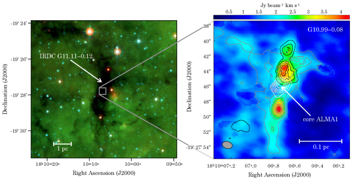
Figure 1: Locations of the IRDC G11.11$-$0.12, the clump G10.99$-$0.08 and the core ALMA1. Left panel: Three-colour view of the vicinity of the IRDC G11.11$-$0.12 obtained with Spitzer IRAC and MIPS data with 5.8 $\mu$m (blue), 8.0 $\mu$m (green), 24.0 $\mu$m (red) from the GLIMPSE and MIPSGAL survey (Churchwell et al., 2009; Carey et al., 2009). Right panel: Moment-0 of the CO($J$=2$\rightarrow$1) emission integrated over the velocity range $-28$$<$v_LSRK(km s^-1)$<$+104. The image includes only pixels with a brightness in the range 4-250 mJy beam^-1. The white contours indicate the 1.3 mm continuum emission. The contours are rms$\times$2$\times$$i$, with rms=$1.5\times 10^{-4}$ Jy beam^-1 and $i$=3,4,5$\ldots$ The black and grey contours represent velocity-integrated emission in the velocity range $-28$$<$v_LSRK(km s^-1)$<$+26 and +26$<$v_LSRK(km s^-1)$<$+104, respectively. The contours are rms$\times$2$\times$$i$, with rms=$1.8\times 10^{-1}$ Jy beam^-1 km s^-1 and $i$=3,4,5$\ldots$ The filled ellipse located at the bottom–left corner represents the size of the synthesized beam, $\theta_{\rm FWHM}$=1$\hbox to0.0pt{.\hss}^{\prime\prime}$38$\times$0$\hbox to0.0pt{.\hss}^{\prime\prime}$95, P.A.=76^∘.

In the ALMA Survey of 70 $\mu$m Dark High-mass Clumps in Early Stages (ASHES: Sanhueza et al., 2019) we investigate the early stages of high-mass star formation using the Atacama Large Millimeter/submillimeter Array (ALMA). In a pilot survey, we carried out high-angular resolution observations towards 12 massive 70 $\mu$m dark clumps. The sample was selected by combining the ATLASGAL survey (Schuller et al., 2009; Contreras et al., 2013) and a series of studies from the MALT90 survey (Foster et al., 2011; Sanhueza et al., 2012; Foster et al., 2013; Jackson et al., 2013; Guzmán et al., 2015; Rathborne et al., 2016; Contreras et al., 2017; Whitaker et al., 2017). The source selection and fragmentation properties of the sample are described in detail by Sanhueza et al. (2019).

One of the ASHES targets is the clump G010.991$-$00.082 (hereafter, G10.99$-$0.08), which is located at the distance of 3.7 kpc (Pillai et al., 2006; Henning et al., 2010; Kainulainen et al., 2013; Wang et al., 2016; Sanhueza et al., 2019; Pillai et al., 2019, and references therein). This clump has no point sources detected in the near or mid-infrared either in the GLIMPSE nor in the MIPS Galactic Plane Survey (Churchwell et al., 2009; Carey et al., 2009). Neither does it have point sources detected at 70 $\mu$m in the HiGAL survey (Molinari et al., 2010), indicating that this clump is at a very early stage of its evolution (e.g. Sanhueza et al., 2013; Tan et al., 2013; Sanhueza et al., 2017). A SED fitting for G10.99$-$0.08 gives a dust temperature of 12 K and a mass of 1810 $M_{\odot}$ (Sanhueza et al., 2019). Recently, Pillai et al. (2019) presented SMA observations toward G10.99$-$0.08 and identified structures that seem to be molecular outflows driven by low-mass protostars. Li et al. (2020) confirmed the presence of blue- and red-shifted emission associated with the brightest core (ALMA1; $M\sim 10M_{\odot}$) suggesting that it is indeed driving a bipolar outflow, although, given the complexity of the emission in the region, it was not possible to characterise in detail the observed structures. Nevertheless, since G10.99$-$0.08 is a relatively young star-forming region, it is an attractive target that deserves further investigation to study the first stages of development of molecular outflows in a relatively massive core that has the potential to form a high-mass star in the future.

As part of the series of papers derived from the ASHES survey, here we present an analysis of the CO ($J$=2$\rightarrow$1) line emission observed with ALMA toward G10.99$-$0.08 to study in detail the morphology and kinematics of the bipolar molecular outflow associated with core ALMA1, whose P-V diagram exhibits a peculiar $\mathsf{S}$-shaped morphology that has not been seen in other molecular outflows before. A summary of the details of the observations used in this work is presented in §2. The description of the analysis of the data and the presentation of a spatio-kinematical model that explains the observations are given in section §3. In section §4 we discuss the physical interpretation of the spatio-kinematical model and estimate the age and energetics of the molecular outflow. In this section we also discuss on the nature of the driving jet. Finally, the conclusions of this work are presented in section §5

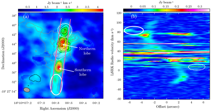
Figure 2: ALMA observations of the CO($J$=2$\rightarrow$1) emission in G10.99$-$0.08. (a) Same as right panel of Fig. 1. (b) P-V diagram of the CO($J$=2$\rightarrow$1) emission obtained by using the slit indicated with parallel pink lines shown in the left panel. The horizontal axis is the position offset with respect to the position of the continuum peak of the core ALMA1, (J2000) R.A.=18^h10^m06$\hbox to0.0pt{.\hss}^{\rm s}$736, Dec.=$-$19^∘27^′45$\hbox to0.0pt{.\hss}^{\prime\prime}$88. The ellipses indicate emission aligned in the direction connecting the northern and southern lobes but that does not follow the $\mathsf{S}$-shaped pattern associated with the bright lobes (see main text).

2 Observations

The observations used in the present analysis were carried out on January 28, 2016 using 41 antennas of the ALMA 12m array with Band 6 receivers ($\sim$224 GHz; 1.34 mm) as part of the project 2015.1.01539.S (P.I.: P. Sanhueza). The array was arranged in configuration C36-1 and the maximum and minimum baseline lengths were 330 m and 15 m, respectively. The corresponding angular resolution and maximum recoverable scale are 0$\hbox to0.0pt{.\hss}^{\prime\prime}$95 and 8$\hbox to0.0pt{.\hss}^{\prime\prime}$8, respectively. The data were calibrated manually with CASA using J1924-2914 (3.05 Jy) and J1733-1304 (1.65 Jy) as bandpass and gain calibrators, respectively. The flux was calibrated using Titan. The continuum emission was produced by averaging line-free channels in visibility space (see additional details for the continuum in Sanhueza et al., 2019). Channel maps of the CO ($J$=2$\rightarrow$1) line with a spectral resolution of $\sim$1.3 km s^-1 were created after subtracting the continuum emission from the data cubes. The imaging of the channel maps was performed setting the multi-scale option value to 0, 5, 15, and 25 times the size of the pixel of 0$\hbox to0.0pt{.\hss}^{\prime\prime}$2. The selection of masks for cleaning was done automatically using the cleaning algorithm yclean developed by Contreras et al. (2018). The Briggs weighting robust parameter was set to 0.5, which resulted in a final angular resolution for the images of 1$\hbox to0.0pt{.\hss}^{\prime\prime}$38$\times$0$\hbox to0.0pt{.\hss}^{\prime\prime}$95, PA=76^∘ ($\sim$0.025 pc at 3.7 kpc). The typical channel root-mean-square (rms) noise level in the resulting channel maps is $\sim$4 mJy beam^-1.

3 Data analysis and Results

The clump G10.99$-$0.08 is embedded in the IRDC G11.11$-$0.12, as it is shown in Fig. 1. Pillai et al. (2019) presented observations carried out with the SMA toward G10.99$-$0.08, with an angular resolution of $\sim$4^′′ ($\sim$0.07 pc at 3.7 kpc), and found hints of the presence of a molecular outflow in this clump. Particularly, in their Figure 2 there is blue- and red-shifted CO($J$=2$\rightarrow$1) line emission distributed in a more or less bipolar fashion and centred at the position of the brightest 1.3 mm continuum peak (core ALMA1). Li et al. (2020) confirmed the presence of such a bipolar structure, which they identified as a bipolar outflow associated with core ALMA1. The ALMA observations of the CO($J$=2$\rightarrow$1) line emission presented in this work clearly reveal two bright lobes located toward the north and south of core ALMA1 (see right panel of Fig. 1).

The colour map in the right panel of Fig. 1 is a moment-0 image of the emission integrated over the velocity range $-28$$<$v_LSRK(km s^-1)$<$+104, which, as it is shown below, includes all the CO($J$=2$\rightarrow$1) emission associated to the bipolar outflow, and the white contours indicate the 1.3 mm continuum emission. The moment-0 image was created using only pixels with a brightness in the range 4-250 mJy beam^-1 to enhance the emission of the bipolar outflow, nonetheless some extended emission from the ambient medium is also visible in the image. The black and grey contours represent velocity-integrated emission in the velocity range $-28$$<$v_LSRK(km s^-1)$<$+26 and +26$<$v_LSRK(km s^-1)$<$+104, respectively. The derived systemic velocity of the bipolar outflow is v_sys,LSRK=26.1 km s^-1 (see below). Thus, the gas of the northern lobe is moving toward us, while the southern lobe is moving away from us.

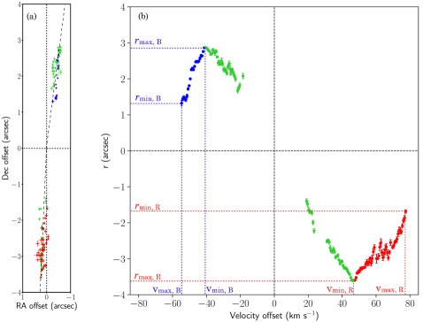
Figure 3: Spatial and velocity distribution of the CO($J$=2$\rightarrow$1) emission in G10.99$-$0.08. (a) Peak positions of the CO($J$=2$\rightarrow$1) emission for each individual velocity channel obtained by fitting a 2D-Gaussian function. The origin corresponds to the peak position of the continuum emission (see main text). The negative R.A. offsets are on the right side of the plot. (b) Position offsets from peak position of the continuum as a function of the velocity offset from the systemic velocity v_sys,LSRK=26 km s^-1. For both panels, the colour of the data points are coded according to their velocity gradient, d$|$v$|$/d$|r|$; green for d$|$v$|$/d$|r|$$>$0 and blue-red for d$|$v$|$/d$|r|$$<$0. The negative distance offsets correspond to data points with negative Declination offsets. The error bars represent the nominal errors from the 2D-Gaussian fit.

In order to scrutinize the spatial distribution and kinematics of the bipolar lobes, we created a P-V diagram using the slit indicated with parallel pink lines in Fig. 2a. The resulting P-V diagram is shown in Fig. 2b. The vertical axis is the LSRK radio velocity and the horizontal axis is the position offset with respect to the position of the 1.3 mm continuum peak, (J2000) R.A.=18^h10^m06$\hbox to0.0pt{.\hss}^{\rm s}$736, Dec.=$-$19^∘27^′45$\hbox to0.0pt{.\hss}^{\prime\prime}$88. The P-V diagram reveals an $\mathsf{S}$-shaped feature crossed by several horizontal components. Inspection of individual channels in the data cube shows that the horizontal components are due to extended emission of the ambient gas. On the other hand, the $\mathsf{S}$-shaped feature is associated with emission from the bipolar lobes seen in Fig. 2a. It is worth noting that there is emission that extends northward and southward of the two bright lobes, which is indicated in Fig. 2a with a dashed and a solid oval, respectively. The corresponding emission in the P-V diagram is also indicated with a dashed and a solid oval (see Fig. 2b). It can be seen that such emission does not follow the $\mathsf{S}$-shaped pattern associated with the bright lobes, implying that it is most likely arising in the gas of the ambient medium.

Interestingly, the $\mathsf{S}$-shaped pattern in the P-V diagram of Fig. 2b resembles the P-V diagram of the evolved star IRAS 16342$-$3814 (Sahai et al., 2017; Tafoya et al., 2019). Given the similarity of those two P-V diagrams, we undertook an analysis of data of G10.99$-$0.08 adopting the approach taken by Tafoya et al. (2019), which is described in the following.

Firstly, from the data cube of the CO($J$=2$\rightarrow$1) line we measured the flux density and peak position of the emission associated with the bipolar lobes in every single channel within the velocity range $-28$$<$v_LSRK(km s^-1)$<$+104, which includes all the emission of the $\mathsf{S}$-shaped pattern of the P-V diagram, except the channels with significant contamination from extended emission. Given that the emission in individual channels is not well resolved, we fitted a 2D-Gaussian function to obtain the peak positions. Subsequently, we calculated the separation of the emission peak positions from the peak position of the 1.3 mm continuum, which is defined as the reference position. In Fig. 3a we plot the declination (Dec.) and right ascension (R.A.) offsets of the emission peak positions with respect to the reference position. The points appear clustered in two elongated structures that correspond to the northern and southern lobes. A linear fit to the distribution of points in each of the lobes reveals that while the points of the northern lobe lie on a line with P.A.=$-$8^∘, the points of the southern lobe lie on a line with P.A.=$-$2^∘. In Fig. 3b we plot the distance of the emission peak from the reference position, $r=\pm({\rm Dec.offset}^{2}+{\rm R.A.offset}^{2})^{1/2}$, as a function of the velocity offset with respect to the reference velocity. We took the negative solution of the square root for data points whose Dec. offset is negative. Initially, the systemic velocity reported in previous works (Sanhueza et al., 2019; Pillai et al., 2019) was used as the reference velocity to calculate the velocity offsets. However, the reference velocity was later redefined in such a way that a linear fit of the green points in Fig. 3b (see below for the definition of the colouring code) passes through the origin of the plot. The resulting reference velocity has a value of v_ref,LSRK=26.1 km s^-1, and it is defined as the systemic velocity of the outflow. The physical justification for interpreting the reference velocity in this manner is further discussed in §4.

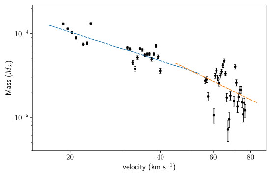
Figure 4: Molecular mass as a function of expansion velocity (mass spectrum) obtained from the emission that is red-shifted with respect to the systemic velocity. The error bars were obtained using the rms noise of the individual channels of 4 mJy beam^-1. The light-blue and orange dashed lines are power-law fits to the data in the velocity ranges 10$<$v_offset(km s^-1)$<$50, and 50$<$v_offset(km s^-1)$<$80, respectively.

In a similar way to the results obtained by Tafoya et al. (2019), the data points shown in Fig. 3b reveal two kinematical components: one with intermediate velocities offsets, in the range $-41$$<$v_offset(km s^-1)$<$+48, and whose velocity gradient is positive, i.e., d$|$v$|$/d$|$$r$$|$ $>$ 0; and another component with higher velocity offsets, in the ranges $-54$$<$v_offset(km s^-1)$<$$-41$ and +48$<$v_offset(km s^-1)$<$+78, and whose velocity gradient is negative. The data points in Fig. 3b are colour-coded according to their velocity gradient: green for d$|$v$|$/d$|$$r$$|$$>$0 and blue or red for d$|$v$|$/d$|$$r$$|$$<$0. In accordance with Tafoya et al. (2019), the kinematical component with positive velocity gradient is referred to as “low velocity component” (LVC), since it has relatively lower velocities offsets, and the component with negative velocity gradient, which has higher velocity offsets, is referred to as “high velocity component” (HVC). It is worth noting that, although the LVC is represented with green colour, it contains material that is both blue- and red-shifted with respect to the systemic velocity. From Fig. 3a it can be seen that, similarly to IRAS 16342$-$3814 (see Figure 1 of Tafoya et al., 2019), despite the different kinematical signatures of the LVC and HVC, they appear aligned in the same direction on the sky. On the other hand, the distribution of the data points in Fig. 3b exhibits a morphology that resembles the $\mathsf{S}$-shaped pattern of the emission in the P-V diagram of Fig. 2b, although rotated 90^∘. This is because the emission peak positions lie basically along one single direction, which makes the plot of Fig. 3b equivalent to a P-V diagram.

4 A molecular outflow driven by a decelerating jet from core ALMA1

The simplest spatio-kinematical model that, in principle, can explain the morphology of the $\mathsf{S}$-shaped seen in the P-V diagram of Fig. 2b considers a single outflow of material expanding with constant velocity and a large precession angle. In this model, the $\mathsf{S}$-shaped pattern results from the projection effect of the material expanding along different directions. The resulting morphology of the outflow is also an $\mathsf{S}$-shaped bipolar structure with some material moving in directions near the line-of-sight and some other material moving nearly on the plane of the sky (e.g., Sahai et al., 2017). However, Fig. 3a shows that the HVC and LVC are aligned along narrow, linear structures. Thus, in order to simultaneously explain the morphologies of the P-V diagram and the spatial distribution of the emission, the constant-velocity model would require a precession angle $\sim$90^∘, i.e., the outflow would need to be precessing on a plane that is oriented almost perfectly perpendicular to the plane of the sky, which is very unlikely. Furthermore, this model neglects the fact that the velocity of the gas in the outflow would depend on the hydrodynamic interaction with ambient gas.

Other typical outflow models, such as the unified wind-driven model that includes a collimated as well as wide opening angle wind (e.g., Shang et al., 2006; Banerjee & Pudritz, 2006; Machida et al., 2008) predict P-V diagrams that do not resemble the $\mathsf{S}$-shaped pattern seen in Fig. 2b (see e.g., Hirano et al., 2010). Similarly, spatio-kinematical models such as biconical outflows (e.g., Cabrit & Bertout, 1986, 1990) and expanding bipolar bubbles (e.g., Shu et al., 1991; Masson & Chernin, 1992), can be easily ruled out since the resulting morphologies of their P-V diagram differs from the ones seen in Fig. 2b.

Tafoya et al. (2019) demonstrated that it is possible to explain the spatial distribution and $\mathsf{S}$-shaped P-V diagram of the CO($J$=2$\rightarrow$1) line emission of the evolved star IRAS 16342$-$3814 with a spatio-kinematical model that includes two components: i) a collimated high-velocity component that decelerates with distance from the central source and ii) a coaxial slower and less collimated component whose velocity increases with distance from the central source. As mentioned in the previous section, §3, the outflow of core ALMA1 has components with the same kinematical characteristics of those of the evolved star IRAS 16342$-$3814. In addition, the morphologies of the spatial distributions and the P-V diagrams of both sources exhibit remarkable similarities. Thereby, we propose that the CO($J$=2$\rightarrow$1) line emission of the outflow of core ALMA1 can be explained by the spatio-kinematical model presented by Tafoya et al. (2019) .

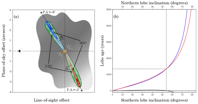
Figure 5: (a) Schematic representation of the spatio-kinematical model of the molecular outflow of core ALMA1 in G10.99$-$0.08. The green region indicates the LVC, whose velocity increases with distance from the central source. The blue and red regions indicate the HVC, which decelerates as a function of distance from the central source. The observer is located on the left side of the diagram. (b) Kinematical age of the blue- and red-shifted parts of the HVC, as function of their inclination angle, obtained from Equation A1. The blue and red solid lines correspond to the blue- and red-shifted part of the HVC, respectively. The black line indicates the difference between the blue and red lines. The ages were calculated assuming a relative inclination of the lobes of ($\theta_{\rm B}-\theta_{\rm R}$)=6^∘. The vertical dashed line indicates the absolute inclination angles of the lobes for which their ages are equal, $\tau$=1300 years. The age is indicated by the horizontal dashed line.

The physical interpretation of the spatio-kinematical model that Tafoya et al. (2019) proposed for IRAS 16342$-$3814 is given in terms of a jet-driven molecular outflow in which the HVC corresponds to molecular gas entrained along the sides of the jet (steady-state entrainment; De Young, 1986; Chernin et al., 1994), and the LVC is associated with entrained material that carries momentum transferred through the leading bow shock (prompt entrainment). This interpretation is supported by the results of Smith et al. (1997), who carried out numerical simulations of jet-driven bipolar outflows and obtained two kinematical components that correspond to the HVC and LVC seen in IRAS 16342$-$3814 and G10.99$-$0.08 (see their Figure 4). Although it should be noted that in their simulations the speed of the HVC remains constant across the outflow, thus the P-V diagram has a $\mathsf{Z}$ -shaped, instead of an $\mathsf{S}$-shaped, morphology. Another piece of evidence that is consistent with the jet-driven outflow interpretation is the profile of the mass spectrum, $m$(v), since it has been found that such outflows exhibit a power-law variation of mass with velocity, i.e., $m(\rm v)$$\propto$v^-γ (Raga & Cabrit, 1993; Lada & Fich, 1996; Cabrit et al., 1997, and references therein). We obtained the mass spectrum of the outflow of core ALMA1 and it is shown in Fig. 4. The molecular mass was calculated using the measured flux density of the CO($J$=2$\rightarrow$1) emission from the outflow in channels with no contamination by emission of the ambient material. Since the blue-shifted lobe seems to be suffering more contamination by emission of the ambient material, Fig. 4 shows only the mass spectrum of the red-shifted lobe. Optically thin emission, LTE conditions, an excitation temperature of $T_{\rm ex}$=12 K (Sanhueza et al., 2019; Li et al., 2020), and a fractional abundance of CO relative to H₂ $f$(CO)=10^-4 were assumed in the calculations. The points exhibit significant spread but they indicate that the data can be described by a double power-law, $m$(v)$\propto$v^-γ, with $\gamma$=1.15$\pm$0.03 (Pearson’s correlation coefficient $r$=$-$0.78) for v_offset$<$50 km s^-1 (LVC), and $\gamma$=1.75$\pm$0.20 ($r$=$-$0.40) for v_offset$>$50 km s^-1 (HVC). This double power-law is predicted by the numerical simulations of jet-driven bipolar outflows (Smith et al., 1997). The slopes of the power law of the outflow of core ALMA1 are slightly shallower than those of other sources (e.g., Rodriguez et al., 1982), but it has been found that the slope steepens with age and energy in the flow (Richer et al., 2000). Thus, the shallower slopes in Fig. 4 would agree with the values expected for a young outflow embedded in a 70 $\mu$m dark massive clump at the early stages of high-mass star formation. Moreover, Solf (1987) proposed a similar model to explain the spatio-kinematical properties of the jet associated with the source HH24-C in the low-mass HH24 complex. As Solf (1987) mentions, the shape of the P-V diagram of HH24-C, obtained from one half of the outflow, resembles that of the Greek capital letter $\Lambda$. This is exactly the shape of the P-V diagram for each of the lobes of core ALMA1 (see Fig. 3b). In addition, from Fig. 3b it can be seen that the velocities at the tips of the lobes are the same for both HVC and LVC, strongly suggesting that there is a common mechanism that drives them simultaneously. Given all these arguments, we conclude that the bipolar lobes seen in core ALMA1 are very likely due to the presence of a young jet-driven molecular outflow.

Finally, we point out that, under this interpretation, the green points in Fig. 3b would correspond to the entrained material whose velocity field follows a Hubble-law, as it is seen in several other molecular outflows. Thus, the velocity offset at the origin of the outflow is expected to be close to zero, which justifies the definition of the velocity reference given in the previous section §3.

4.1 Timescale of the molecular outflow

Fig. 3b shows the current configuration of positions and velocities for the different parts of the molecular outflow of core ALMA1. As Tafoya et al. (2019) pointed out, this type of plot only provides an instantaneous picture of the velocity field in the outflow at present time and cannot be used to trace the velocity history of the gas, unless the deceleration law as a function of time is known for each part of the outflow. Nonetheless, despite of this limitation, important information of the kinematics of the outflow can be extracted by making some reasonable assumptions, which we describe in the following. From Fig. 3b it can be seen that the blue- and red-shifted parts of the HVC have material moving with a maximum velocity, v_max,[B,R] at the minimum position offset, r_min,[B,R], where the subscripts $\rm[B,R]$ stand for blue- and red-shifted part, respectively. Correspondingly, the minimum velocity, v_min,[B,R], is reached at the maximum position offset, r_max,[B,R]. This means that, if one assumes that the driving jet has been launched with a constant velocity throughout its life, the material located at the tip of the jet has suffered a deceleration. Thus, using the size of the HVC and assuming a constant deceleration, the age of the outflow can be estimated. However, before attempting to estimate the age of the outflow, some considerations on its geometrical characteristics are necessary.

Table 1: Physical parameters for the kinematical components in the molecular outflow of core ALMA1

Component	$M$	$p$	$E_{\rm k}$	$\dot{M}$	$F_{\rm m}$	$L_{\rm m}$
Designation	$M_{\odot}$	$M_{\odot}$ km s-1	ergs	$M_{\odot}$ yr-1	$M_{\odot}$ km s-1 yr-1	$L_{\odot}$
HVC	1.7-2.0$\times$10-3	1.1-1.3$\times$10-1	7.1-8.5$\times$1043	1.9-2.3$\times$10-6	1.2-1.5$\times$10-4	6.9-8.2$\times$10-1
LVC	2.6-3.6$\times$10-3	0.9-1.2$\times$10-1	3.2-4.2$\times$1043	3.0-4.2$\times$10-6	1.0-1.4$\times$10-4	3.1-4.0$\times$10-1
Northern Lobe	2.2-3.0$\times$10-3	1.0-1.2$\times$10-1	4.6-5.7$\times$1043	2.5-3.4$\times$10-6	1.1-1.4$\times$10-4	4.3-5.3$\times$10-1
Southern Lobe	2.0-2.7$\times$10-3	1.0-1.2$\times$10-1	5.8-7.0$\times$1043	2.4-3.2$\times$10-6	1.2-1.5$\times$10-4	5.7-6.9$\times$10-1
Combined	4.2-5.7$\times$10-3	2.0-2.4$\times$10-1	1.0-1.3$\times$1044	4.9-6.6$\times$10-6	2.3-2.9$\times$10-4	1.0-1.2

Note. — The values were calculated assuming an inclination of the northern and southern lobes $\theta_{\rm R}$=54^∘, $\theta_{\rm B}$=60^∘, respectively, and an excitation temperature in the range $T_{\rm ex}$=10-30 K. The physical parameters are computed as follows: $M$=$\sum{M_{i}}$, $p$=$\sum{M_{i}{\rm v}_{i}}$, $E_{\rm k}$=$\sum{(M_{i}{\rm v}_{i}^{2}})/2$, $\dot{M}$=$\sum{M_{i}}$/$\Delta\tau$, $F_{\rm m}$=$p$/$\Delta\tau$ and $L_{\rm m}$=$E_{\rm k}$/$\Delta\tau$, where the subscript $i$ is the channel number and $\Delta\tau$ is the time that it takes to the gas to move from r_min,[B,R] to r_max,[B,R].

One characteristic of the outflow of core ALMA1 that is readily seen from Fig. 3 is that the northern and southern lobes have different spatial extents as well as different velocity offsets. While the maximum position offset for the southern lobe is 3$\hbox to0.0pt{.\hss}^{\prime\prime}$7, it is only 2$\hbox to0.0pt{.\hss}^{\prime\prime}$9 for the northern lobe. Similarly, the maximum velocity offsets for the southern and northern lobes are 78 km s^-1 and 54 km s^-1, respectively. However, these values are only projections of the position offset onto the plane of the sky and the velocity offset onto the line-of-sight direction, respectively, implying that the difference of size and velocity offset between the northern and southern lobes could be due to projection effects, i.e., one lobe may be more inclined than the other. Consequently, the inclination angles of the lobes, $[\theta_{\rm B},\theta_{\rm R}]$, with respect to the plane-of-the-sky are needed to calculate the intrinsic values of the size and velocity offset (see Fig. 5a). In Appendix §A we show that it is possible to constrain the relative inclination of the lobes ($\theta_{\rm B}-\theta_{\rm R}$), which can then be used to further constrain their absolute inclination, by assuming that the launch velocity of the driving jet is the same for both lobes, i.e., v_i,B=v_i,R=v_i, and that the blue- and redshifted parts of the jet have the same age, i.e., $\tau_{\rm jet,B}$=$\tau_{\rm jet,R}$=$\tau$. In the following subsection, §4.2, we provide arguments that support these assumptions.

Using the observed values of the projected sizes and line-of-sight velocities of the lobes, it is found that their relative inclination angle is restricted to the range 0^∘$<$($\theta_{\rm B}-\theta_{\rm R}$)$<$9.5^∘. Furthermore, for each given value of ($\theta_{\rm B}-\theta_{\rm R}$), there are only two pairs of inclination angles for the lobes. For example, if ($\theta_{\rm B}-\theta_{\rm R}$)=1^∘, the inclination angles of the northern and southern lobes are either [$\theta_{\rm B}$=85^∘, $\theta_{\rm R}$=84^∘] or [$\theta_{\rm B}$=3^∘, $\theta_{\rm R}$=2^∘] (see Table 2). This means that if we assume that the lobes are almost aligned with each other, their axis would lie basically either on the line-of-sight direction or on the plane-of-the-sky. However, this is an unlikely configuration since it would imply either unrealistic initial velocities and extremely short kinematical time scales, or too large sizes for the lobes (see Table 2). On the other hand, if one considers an average inclination of the lobes equal to the mean inclination angle, ($\theta_{\rm B}+\theta_{\rm R}$)/2=57.3^∘ (e.g., Bontemps et al., 1996; Beuther et al., 2002; de Villiers et al., 2014), equation A2 gives a relative angle of ($\theta_{\rm B}-\theta_{\rm R}$)$\approx$6^∘ and the resulting age and size of the outflow are $\approx$1300 years and $\approx$0.2 pc, respectively (see Fig. 5b).

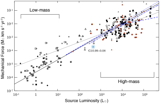
Figure 6: Mechanical force as a function of bolometric luminosity. The plot has been adapted from Figure 7 of Maud et al. (2015), Figure 4 of Beuther et al. (2002) and Figure 4 of Zhang et al. (2005). The blue asterisk indicates the value for the outflow of core ALMA1.

4.2 Energetics of the molecular outflow

From Table 2 it can be seen that regardless of the relative inclination between the lobes, the final velocity of the northern lobe, v_f,B, is lower than that of the southern lobe, v_f,R. This difference could simply be indicating that the southern part of the jet is intrinsically faster than the northern part, or it could be indicating that the later is preferentially decelerated by ambient material. One way of investigating whether the initial velocities and ages for both parts of the jet are indeed equal or not is by means of comparing the momentum and mechanical force carried by the lobes. If the launch velocities and ages are the same for both parts of the jet, the momentum and mechanical force for both lobes should be the same too.

In order to calculate the energetics of the molecular outflow of core ALMA1, we followed the same procedure as Tafoya et al. (2019). Firstly, we assumed that all the velocity vectors within each lobe are parallel to the outflow axis, thus their de-projected magnitude is v$=$v${}_{\rm offset}/{\rm sin}\,\theta_{\rm inc}$. We adopted an inclination of the lobes $\theta_{\rm R}$=54^∘, $\theta_{\rm B}$=60^∘, which, as discussed in the previous subsection, §4.1, results in an age of the outflow of $\tau_{\rm jet}$=1300 years. Subsequently, we calculated the values of the physical parameters shown in Table 1 for each individual velocity channel, $i$, assuming LTE conditions, optically thin emission and an excitation temperature in the range $T_{\rm ex}$=10-30 K. Finally, we added the values of the channels that correspond to a particular component, namely northern lobe, southern lobe, HVC and LVC. The entrainment rate, $\dot{M}$, mechanical force, $F_{\rm m}$, and mechanical luminosity, $L_{\rm m}$, were calculated using the times that it takes to the gas to move from r_min,[B,R] to r_max,[B,R], which are estimated to be 850 and 800 yr for the red- and blue-shifted lobe, respectively. The resulting values of the physical parameters are listed in Table 1. The derived molecular mass for the outflow is lower than the one estimated by Pillai et al. (2019), but their observations had lower angular resolution and were more affected by contamination of emission of the ambient material. As a matter of fact, in our analysis we do not consider the emission at the base of the outflow because of contamination of emission of the ambient material (see Fig. 2b). Thus, the values of the molecular mass shown in Table 1 should be considered as lower limits. Nevertheless, using the mass ($M$$\sim$10 $M_{\odot}$; Sanhueza et al., 2019; Pillai et al., 2019) and bolometric luminosity ($L_{\rm bol}$$\sim$470 $L_{\odot}$) for core ALMA1, and taking our estimation of the total mechanical force from Table 1, which is a dynamical quantity that is not significantly affected by a poor sampling of the outflow, we find that core ALMA1 follows the mechanical force versus core mass and bolometric luminosity correlations obtained from molecular outflows in low- and high-mass star-forming regions (see Fig.6).

In addition, the values of the momentum and mechanical force for the northern and southern lobes listed in Table 1 are, within the uncertainty range, basically the same. Thus, we conclude that, even though the final velocities of the northern and southern lobes are different, they must have been ejected simultaneously and with the same initial velocity, as suggested in §4.1.

4.3 Nature of the deceleration of the HVC

There is now a plethora of observations of molecular outflows in low and high-mass star-forming regions that have revealed a rich variety of spatio-kinematical properties (e.g., Bachiller, 1996; Arce et al., 2007; Kong et al., 2019; Zapata et al., 2019; Nony et al., 2020; Lee, 2020; Li et al., 2020). As mentioned before, it is common that collimated molecular outflows exhibit components with a Hubble-law velocity profile and/or complex Hubble wedges, some of which may contain decelerating knots (e.g., Bachiller et al., 1990; Plunkett et al., 2015; Nony et al., 2020). Nevertheless, to the best of our knowledge, there has not been reported in the literature any other molecular outflow in a star-forming region whose P-V diagram has the $\mathsf{S}$-shaped morphology seen in G10.99$-$0.08. Particularly, the part of the P-V diagram that corresponds to the decelerating HVC, which we interpret as entrained material along the sides of the jet, is not seen in other outflows. One may wonder what is the origin of the deceleration of the HVC and what are the particular physical conditions of the molecular outflow of core ALMA1 that result in such a peculiar P-V diagram. The driving jet of the outflow, in principle, could be launched magnetocentrifugally, as it is proposed in the unified wind-driven model (Shang et al., 2006), although without the wide opening angle component (or with one that is too weak to be detected). Given the short age of the outflow of ALMA1 ($\sim$1000 years), it could be argued that the presence of the decelerating HVC occurs mainly at an early phase of the outflow when there is more material available to be entrained along the sides of the jet, i.e., the jet has not completely cleared out the inner parts of the lobes. However, similar time-scales have been estimated for outflows of cores with a wide range of masses (1-100 $M_{\odot}$, Nony et al., 2020) and they do not show the $\mathsf{S}$-shaped morphology seen in the outflow of core ALMA1. Consequently, the short age of the outflow does not seem to be the only factor for having such a P-V diagram. Chernin et al. (1994) found that a jet with Mach number $\leq$6 slows down rapidly by delivering energy and momentum as it entrains ambient material along its sides, which would account for the deceleration of the HVC. We thus propose that the observed deceleration of the HVC is likely due to the presence of a jet with a low Mach number that decelerates as it interacts with the ambient material. We also note that, given that the energetics of the outflow of core ALMA1 do not deviate from the trend seen in other outflows (Bontemps et al., 1996; Beuther et al., 2002; Zhang et al., 2005), future observations with high angular resolution should reveal more outflows with characteristics similar to that of G10.99$-$0.08.

On the other hand, we have so far assumed that the driving jet has been launched with a constant velocity throughout its life. However, an alternative possibility that could explain the observed deceleration of the HVC is that the parts of the jet launched at earlier times (the ones further away from the protostar) were ejected at a lower velocity than those launched at later times (the ones closer to the protostar). This interpretation would imply that the jet is not ejected at a constant velocity, possibly shedding some light on the mass-accretion rate of the protostar, as we describe in the following. Since we do not know exactly the evolutionary stage of the protostar on the pre-main sequence track, we assume the accreting protostar is at ZAMS for the sake of estimating its mass. Considering the bolometric luminosity of the clump G10.99$-$0.08, $L_{\rm bol}$$\sim$470 $L_{\odot}$, and ignoring the contribution of the accretion luminosity $L_{\rm acc}$, i.e., $L_{\rm acc}$ $<$ $L_{\star}$, which is valid for more massive stars with typical accretion rates, the ZAMS mass of the star would be $M_{\rm ZAMS}$$\approx$5 $M_{\odot}$ (Schaller et al., 1992). This implies that the current mass of the protostar is $\lesssim$5 $M_{\odot}$, assuming that all the luminosity from the clump is produced by a single protostar. Typically, one can consider that the initial velocity of the jet is comparable to the Keplerian velocity of the accretion disk at the jet launching location Pelletier & Pudritz (1992). Therefore, the increase in jet speed over time would imply an increase in dynamical mass of the central object over time, if assuming that the jet is launched at the same location (e.g., see Figure 6 from Rosen & Krumholz, 2020). Based on the velocity differences seen in Fig. 3, the increase of dynamical mass, which is proportional to (v_max/v_min)², would be a factor of 2-3 times the initial mass. This would mean that there has been a significant increase in protostellar mass over the time scale of $\sim$1000 years, implying an upper limit for the mass-accretion rate of $\lesssim$2$\times$10^-3$M_{\odot}$ yr^-1. This value is rather large considering the physical parameters of the outflow listed in Table 1, which makes it unlikely that the increase of the jet speed over time is due only to the increase in dynamical mass of the central object. Nonetheless, the combined effect of not having a constant launch velocity together and deceleration of the jet by the entrained material may explain the $\mathsf{S}$-shaped P-V diagram of this source.

In order to further explore these possibilities and to better understand the physical characteristics of molecular outflows that exhibit a decelerating HVC, observations with higher angular resolution, together with new models and numerical simulations, will be crucial. Recently, Tafoya et al. (2020) obtained high resolution images with ALMA of a jet-driven molecular outflow in the the evolved star W43A, which also exhibits an $\mathsf{S}$-shaped P-V diagram. The sharp images allowed them to clearly disentangle the different components of the molecular outflow, revealing an extremely collimated decelerating HVC. Future observations with higher angular resolution may allow us to unveil the structure of the molecular outflow of core ALMA1 too.

5 Conclusions

In this work we have carried out a spatio-kinematical analysis of the CO($J$=2$\rightarrow$1) line emission of the molecular outflow associated with the relatively massive core ALMA1 embedded in G10.99$-$0.08. The P-V diagram has a peculiar $\mathsf{S}$-shaped morphology that is explained by means of two components with different kinematical characteristics: an inner axial high-velocity component that moves with high velocity but decelerates, and a co-axial component moving with lower velocity but whose velocity increases with distance from the central source. The spatio-kinematical model is interpreted as a jet-driven molecular outflow. The high-velocity decelerating component is associated with material moving near in the axis of the flow entrained by the underlying jet, or it could be the molecular component of the jet itself. The lower velocity component is interpreted as material lying in zones further away from the axis of the flow ambient but because of the entrainment by the inner gas it appears as if it was being accelerated. This interpretation is supported by the mass spectrum derived from the emission of the molecular gas. From an analysis of the P-V diagram profile we conclude that there is a relative angle between the axis of the the blue- and red-shifted lobes. Assuming an overall mean inclination angle of the outflow of $\approx$57^∘, the relative angle between the lobes is $\approx$6^∘. For such an inclination, the resulting age and size of the outflow are $\approx$1300 years and $\approx$0.2 pc, respectively. Further calculations and numerical simulations are necessary to better understand the physical characteristics of molecular outflows that have $\mathsf{S}$-shaped P-V diagrams. In addition, higher angular resolution observations are necessary to better constrain the input parameters of the models.

Finally, we stress the fact that molecular outflows with very similar spatio-kinematical characteristics to those of the outflow of core ALMA1 are seen in evolved stars too. This shows that, despite being found in different astrophysical contexts, molecular outflows may be studied with a unified approach, which encourages us to develop more synergies between different fields of astronomy to broaden our knowledge on the physical processes underlying their formation and evolution.

Appendix A Appendix

Consider the jet of core ALMA1, traced by the emission of the HVC, moving along a direction that has an inclination angle $\theta_{\rm R,B}$ with respect to the plane of the sky, where the subscripts B and R indicate the blue- and red-shifted part of the jet, respectively (see Fig. 7). If both parts of the jet were launched with the same initial velocity, v_i, and the material at the tip of the jet has slowed down with a constant deceleration to a final velocity, v_f,[B,R], over a distance, $l_{\rm B,R}$, then the travel-time (i.e., the age for each part of the jet), $\tau_{\rm jet[B,R]}$, is given by

$$\tau_{\rm jet,[B,R]}=\frac{2\,l_{\rm B,R}}{{\rm v}_{\rm i}+{\rm v}_{\rm f,[B,R]}}.$$ (A1)

Assuming that the blue- and red-shifted parts of the jet were launched simultaneously, i.e., $\tau_{\rm B}=\tau_{\rm R}$, and considering from Fig. 3 that $l_{\rm B,R}={\rm r}_{\rm max,[B,R]}/{\rm cos}\,\theta_{\rm R,B}$ and v${}_{\rm f,[B,R]}=$v${}_{\rm min,[B,R]}/{\rm sin}\,\theta_{\rm R,B}$, one obtains the following equation:

$$\frac{2\,{\rm r}_{\rm max,B}/{\rm cos}\,\theta_{\rm B}}{{\rm v}_{\rm i}+{\rm v}_{\rm min,B}/{\rm tan}\,\theta_{\rm B}}=\frac{2\,{\rm r}_{\rm max,R}/{\rm cos}\,\theta_{\rm R}}{{\rm v}_{\rm i}+{\rm v}_{\rm min,R}/{\rm tan}\,\theta_{\rm R}}.$$ (A2)

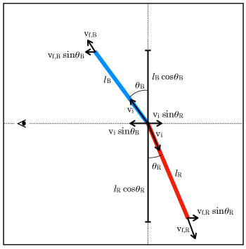
Figure 7: Diagram of the configuration of the blue- and red-shifted parts of the jet in the molecular outflow of G10.99$-$0.08. The initial velocity of the jet, v_i, is assumed to be the same for both parts. The observer is located on the left part of the diagram.

Since the red-shifted part of the jet seems to have suffered less deceleration, the launch velocity can be approximated as v_i$\approx$v${}_{\rm max,R}/{\rm sin}\,\theta_{\rm R}$ and solve numerically $\theta_{\rm B}$=$\theta_{\rm B}(\theta_{\rm R})$ from equation A2. Using the numerical values of r_max,[B,R], v_min,[B,R] and v_max,R from Fig. 3, it is found that equation A2 has real solutions only for 0${}^{\circ}<(\theta_{\rm B}-\theta_{\rm R})<9.5^{\circ}$. Therefore, it can be concluded that the relative inclination angle of the northern and southern lobes is less than $\approx$9.5^∘. Furthermore, for a given difference, ($\theta_{\rm B}-\theta_{\rm R}$), there are only two possible pairs of angles, $\theta_{\rm R,B}$, that solve Equation A2. The values of $\theta_{\rm R,B}$ for given values of ($\theta_{\rm B}-\theta_{\rm R}$) are listed in Table 2. From Table 2 it can be seen that for $(\theta_{\rm B}-\theta_{\rm R})\approx 0$, both $\theta_{\rm R,B}$ are either close to 0^∘, which would imply an initial velocity for the jet of $\sim$2000 km s^-1, or 90^∘, which results in total length of the outflow of $\sim$0.6 pc. It is worth noting that for the relative angle $(\theta_{\rm B}-\theta_{\rm R})\approx 9.5$^∘ there is only one pair of angles that solves equation A2, [$\theta_{\rm R}$=20^∘ and $\theta_{\rm B}$=29.5^∘], which would imply an age of the outflow of $\tau=350$ years.

Table 2: Inclination angle and spatio-kinematical parameters of the blue- red-shifted jets in core ALMA1

($\theta_{\rm B}-\theta_{\rm R}$)	Solution1	$\theta_{\rm R}$	$\theta_{\rm B}$	vi	vf,R	vf,B	$l_{\rm R}$	$l_{\rm B}$	$\tau$
degrees		degrees	degrees	km s-1	km s-1	km s-1	1017 cm	1017 cm	years
1	Sol. 1	84	85	80	48	41	17.7	18.8	9240
	Sol. 2	2	3	2292	1375	783	1.54	1.96	34
2	Sol. 1	78	80	82	49	42	8.86	9.43	4569
	Sol. 2	2	4	2292	1375	588	1.54	1.96	34
3	Sol. 1	72	75	84	50	42	5.95	6.34	2989
	Sol. 2	3	6	1529	917	392	1.55	1.96	51
4	Sol. 1	66	70	88	53	44	4.50	4.82	2181
	Sol. 2	4	8	1147	688	295	1.55	1.96	68
5	Sol. 1	60	65	92	55	45	3.64	3.92	1682
	Sol. 2	6	11	765	459	215	1.57	1.97	102
6	Sol. 1	54	60	99	59	47	3.08	3.33	1337
	Sol. 2	7	13	656	394	182	1.58	1.97	119
7	Sol. 1	48	55	108	65	50	2.68	2.93	1079
	Sol. 2	9	16	511	307	149	1.60	1.98	154
8	Sol. 1	41	49	122	73	54	2.35	2.60	844
	Sol. 2	11	19	419	252	126	1.63	2.00	189
9	Sol. 1	33	42	147	88	61	2.07	2.34	631
	Sol. 2	16	25	290	174	97	1.70	2.04	278

Note. — ¹For each value of ($\theta_{\rm B}-\theta_{\rm R}$) there are two possible combination of solutions for $\theta_{\rm B}$ and $\theta_{\rm R}$ and the respective physical parameters derived from them.

References

- Arce et al. (2007) Arce, H. G., Shepherd, D., Gueth, F., et al. 2007, in Protostars and Planets V, ed. B. Reipurth, D. Jewitt, & K. Keil (Tuscon, AZ: Univ. Arizona Press), 245
- Bachiller (1996) Bachiller, R. 1996, ARA&A, 34, 111
- Bachiller et al. (1990) Bachiller, R., Cernicharo, J., Martin-Pintado, J., Tafalla, M., & Lazareff, B. 1990, A&A, 231, 174
- Bally (2016) Bally, J. 2016, ARA&A, 54, 491
- Banerjee & Pudritz (2006) Banerjee, R., & Pudritz, R. E. 2006, ApJ, 641, 949
- Beuther et al. (2002) Beuther, H., Schilke, P., Sridharan, T. K., et al. 2002, A&A, 383, 892
- Bontemps et al. (1996) Bontemps, S., Andre, P., Terebey, S., & Cabrit, S. 1996, A&A, 311, 858
- Cabrit & Bertout (1986) Cabrit, S., & Bertout, C. 1986, ApJ, 307, 313
- Cabrit & Bertout (1990) —. 1990, ApJ, 348, 530
- Cabrit et al. (1997) Cabrit, S., Raga, A., & Gueth, F. 1997, in IAU Symposium, Vol. 182, Herbig-Haro Flows and the Birth of Stars, ed. B. Reipurth & C. Bertout, 163–180
- Carey et al. (2009) Carey, S. J., Noriega-Crespo, A., Mizuno, D. R., et al. 2009, PASP, 121, 76
- Chernin et al. (1994) Chernin, L., Masson, C., Gouveia dal Pino, E. M., & Benz, W. 1994, ApJ, 426, 204
- Churchwell et al. (2009) Churchwell, E., Babler, B. L., Meade, M. R., et al. 2009, PASP, 121, 213
- Contreras et al. (2017) Contreras, Y., Rathborne, J. M., Guzman, A., et al. 2017, MNRAS, 466, 340
- Contreras et al. (2013) Contreras, Y., Schuller, F., Urquhart, J. S., et al. 2013, A&A, 549, A45
- Contreras et al. (2018) Contreras, Y., Sanhueza, P., Jackson, J. M., et al. 2018, ApJ, 861, 14
- de Villiers et al. (2014) de Villiers, H. M., Chrysostomou, A., Thompson, M. A., et al. 2014, MNRAS, 444, 566
- De Young (1986) De Young, D. S. 1986, ApJ, 307, 62
- Foster et al. (2011) Foster, J. B., Jackson, J. M., Barnes, P. J., et al. 2011, ApJS, 197, 25
- Foster et al. (2013) Foster, J. B., Rathborne, J. M., Sanhueza, P., et al. 2013, PASA, 30, e038
- Guzmán et al. (2015) Guzmán, A. E., Sanhueza, P., Contreras, Y., et al. 2015, ApJ, 815, 130
- Henning et al. (2010) Henning, T., Linz, H., Krause, O., et al. 2010, A&A, 518, L95
- Hirano et al. (2010) Hirano, N., Ho, P. P. T., Liu, S.-Y., et al. 2010, ApJ, 717, 58
- Hirano et al. (2006) Hirano, N., Liu, S.-Y., Shang, H., et al. 2006, ApJ, 636, L141
- Jackson et al. (2013) Jackson, J. M., Rathborne, J. M., Foster, J. B., et al. 2013, PASA, 30, e057
- Kainulainen et al. (2013) Kainulainen, J., Ragan, S. E., Henning, T., & Stutz, A. 2013, A&A, 557, A120
- Kong et al. (2019) Kong, S., Arce, H. G., Maureira, M. J., et al. 2019, ApJ, 874, 104
- Lada & Fich (1996) Lada, C. J., & Fich, M. 1996, ApJ, 459, 638
- Lee (2020) Lee, C.-F. 2020, A&A Rev., 28, 1
- Li et al. (2019a) Li, S., Zhang, Q., Pillai, T., et al. 2019a, ApJ, 886, 130
- Li et al. (2019b) Li, S., Wang, J., Fang, M., et al. 2019b, ApJ, 878, 29
- Li et al. (2020) Li, S., Sanhueza, P., Zhang, Q., et al. 2020, ApJ, 903, 119
- Lu et al. (2015) Lu, X., Zhang, Q., Wang, K., & Gu, Q. 2015, ApJ, 805, 171
- Machida et al. (2008) Machida, M. N., Inutsuka, S.-i., & Matsumoto, T. 2008, ApJ, 676, 1088
- Masson & Chernin (1992) Masson, C. R., & Chernin, L. M. 1992, ApJ, 387, L47
- Maud et al. (2015) Maud, L. T., Moore, T. J. T., Lumsden, S. L., et al. 2015, MNRAS, 453, 645
- Molinari et al. (2010) Molinari, S., Swinyard, B., Bally, J., et al. 2010, PASP, 122, 314
- Nony et al. (2020) Nony, T., Motte, F., Louvet, F., et al. 2020, A&A, 636, A38
- Palau et al. (2006) Palau, A., Ho, P. T. P., Zhang, Q., et al. 2006, ApJ, 636, L137
- Pelletier & Pudritz (1992) Pelletier, G., & Pudritz, R. E. 1992, ApJ, 394, 117
- Pillai et al. (2019) Pillai, T., Kauffmann, J., Zhang, Q., et al. 2019, A&A, 622, A54
- Pillai et al. (2006) Pillai, T., Wyrowski, F., Menten, K. M., & Krügel, E. 2006, A&A, 447, 929
- Plunkett et al. (2015) Plunkett, A. L., Arce, H. G., Mardones, D., et al. 2015, Nature, 527, 70
- Qiu et al. (2008) Qiu, K., Zhang, Q., Megeath, S. T., et al. 2008, ApJ, 685, 1005
- Raga & Cabrit (1993) Raga, A., & Cabrit, S. 1993, A&A, 278, 267
- Rathborne et al. (2016) Rathborne, J. M., Whitaker, J. S., Jackson, J. M., et al. 2016, PASA, 33, e030
- Richer et al. (2000) Richer, J. S., Shepherd, D. S., Cabrit, S., Bachiller, R., & Churchwell, E. 2000, in Protostars and Planets IV, ed. V. Mannings, A. P. Boss, & S. S. Russell (Tuscon, AZ: Univ. Arizona Press), 867
- Rodriguez et al. (1982) Rodriguez, L. F., Carral, P., Ho, P. T. P., & Moran, J. M. 1982, ApJ, 260, 635
- Rosen & Krumholz (2020) Rosen, A. L., & Krumholz, M. R. 2020, AJ, 160, 78
- Sahai et al. (2017) Sahai, R., Vlemmings, W. H. T., Gledhill, T., et al. 2017, ApJ, 835, L13
- Sakai et al. (2013) Sakai, T., Sakai, N., Foster, J. B., et al. 2013, ApJ, 775, L31
- Sanhueza et al. (2010) Sanhueza, P., Garay, G., Bronfman, L., et al. 2010, ApJ, 715, 18
- Sanhueza et al. (2012) Sanhueza, P., Jackson, J. M., Foster, J. B., et al. 2012, ApJ, 756, 60
- Sanhueza et al. (2013) —. 2013, ApJ, 773, 123
- Sanhueza et al. (2017) Sanhueza, P., Jackson, J. M., Zhang, Q., et al. 2017, ApJ, 841, 97
- Sanhueza et al. (2019) Sanhueza, P., Contreras, Y., Wu, B., et al. 2019, ApJ, 886, 102
- Schaller et al. (1992) Schaller, G., Schaerer, D., Meynet, G., & Maeder, A. 1992, A&AS, 96, 269
- Schuller et al. (2009) Schuller, F., Menten, K. M., Contreras, Y., et al. 2009, A&A, 504, 415
- Shang et al. (2006) Shang, H., Allen, A., Li, Z.-Y., et al. 2006, ApJ, 649, 845
- Shu et al. (1991) Shu, F. H., Ruden, S. P., Lada, C. J., & Lizano, S. 1991, ApJ, 370, L31
- Smith et al. (1997) Smith, M. D., Suttner, G., & Yorke, H. W. 1997, A&A, 323, 223
- Solf (1987) Solf, J. 1987, A&A, 184, 322
- Svoboda et al. (2019) Svoboda, B. E., Shirley, Y. L., Traficante, A., et al. 2019, ApJ, 886, 36
- Tafoya et al. (2020) Tafoya, D., Imai, H., Gómez, J. F., et al. 2020, ApJ, 890, L14
- Tafoya et al. (2019) Tafoya, D., Orosz, G., Vlemmings, W. H. T., Sahai, R., & Pérez-Sánchez, A. F. 2019, A&A, 629, A8
- Tan et al. (2013) Tan, J. C., Kong, S., Butler, M. J., Caselli, P., & Fontani, F. 2013, ApJ, 779, 96
- Wang et al. (2016) Wang, K., Testi, L., Burkert, A., et al. 2016, ApJS, 226, 9
- Wang et al. (2011) Wang, K., Zhang, Q., Wu, Y., & Zhang, H. 2011, ApJ, 735, 64
- Whitaker et al. (2017) Whitaker, J. S., Jackson, J. M., Rathborne, J. M., et al. 2017, AJ, 154, 140
- Yang et al. (2018) Yang, A. Y., Thompson, M. A., Urquhart, J. S., & Tian, W. W. 2018, ApJS, 235, 3
- Zapata et al. (2019) Zapata, L. A., Ho, P. T. P., Guzmán Ccolque, E., et al. 2019, MNRAS, 486, L15
- Zhang et al. (2005) Zhang, Q., Hunter, T. R., Brand, J., et al. 2005, ApJ, 625, 864
- Zhang et al. (2015) Zhang, Q., Wang, K., Lu, X., & Jiménez-Serra, I. 2015, ApJ, 804, 141