Vote from the Center: 6 DoF Pose Estimation in RGB-D Images by Radial Keypoint Voting

Abstract

We propose a novel keypoint voting scheme based on intersecting spheres, that is more accurate than existing schemes and allows for fewer, more disperse keypoints. The scheme is based upon the distance between points, which as a 1D quantity can be regressed more accurately than the 2D and 3D vector and offset quantities regressed in previous work, yielding more accurate keypoint localization. The scheme forms the basis of the proposed RCVPose method for 6 DoF pose estimation of 3D objects in RGB-D data, which is particularly effective at handling occlusions. A CNN is trained to estimate the distance between the 3D point corresponding to the depth mode of each RGB pixel, and a set of 3 disperse keypoints defined in the object frame. At inference, a sphere centered at each 3D point is generated, of radius equal to this estimated distance. The surfaces of these spheres vote to increment a 3D accumulator space, the peaks of which indicate keypoint locations. The proposed radial voting scheme is more accurate than previous vector or offset schemes, and is robust to disperse keypoints. Experiments demonstrate RCVPose to be highly accurate and competitive, achieving state-of-the-art results on the LINEMOD ($99.7\%$) and YCB-Video ($97.2\%$) datasets, notably scoring $+4.9\%$ higher ($71.1\%$) than previous methods on the challenging Occlusion LINEMOD dataset, and on average outperforming all other published results from the BOP benchmark for these 3 datasets. Our code is available at http://www.github.com/aaronwool/rcvpose.

1 Introduction

Object pose estimation is an enabling technology for many applications including robot manipulation, human-robot interaction, augmented reality, and autonomous driving [36, 35, 45]. It is challenging due to background clutter, occlusions, sensor noise, varying lighting conditions, and object symmetries.

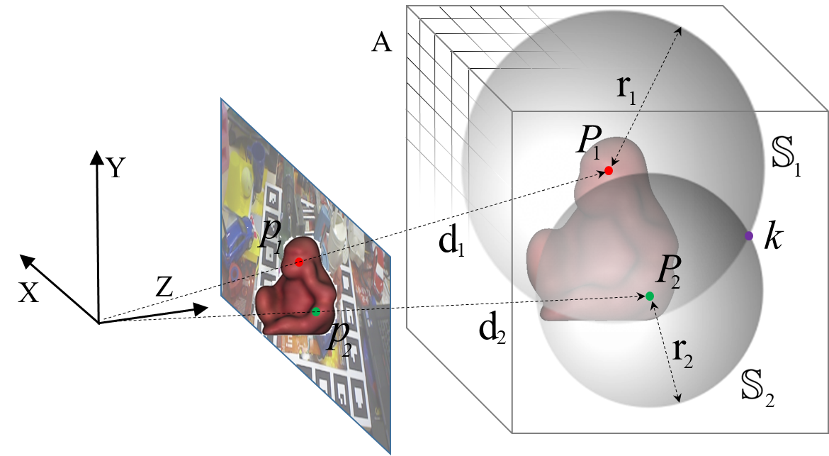
Figure 1: Radial voting scheme: 3D scene point $P_{i}$ at depth d_i projects to 2D image pixel $p_{i}$. The network estimates radial distance r_i from $p_{i}$. Sphere ${\mathbb{S}}_{i}$ is centered at $P_{i}$ with radius r_i, and all accumulator space A voxels on the surface of ${\mathbb{S}}_{i}$ are incremented. Keypoint $k$ lies at the intersection of $\mathbb{S}_{1}\cap\mathbb{S}_{2}$, and all other ${\mathbb{S}}_{i}$

Traditional methods have tackled the problem by establishing correspondences between a known 3D model and image features [15, 40]. They have generally relied on hand-crafted features and therefore fail when objects are featureless or when scenes are very cluttered and occluded [18, 36]. Recent methods use deep learning and train end-to-end networks to directly regress an input image to a 6 DoF pose [19, 49]. For example, CNN-based techniques have been proposed which regress 2D keypoints and use Perspective-n-Point (PnP) to estimate the 6 DoF pose parameters [35, 43]. As an alternate to directly regressing keypoint coordinates, methods which vote for keypoints have been shown to be highly effective [36, 49, 18, 37], especially when objects are partially occluded. These schemes regress a distinct geometric quantity that relates positions of 2D pixels to 3D keypoints, and for each pixel casts this quantity into an accumulator space. As votes accumulate independently per pixel, these methods perform especially well in challenging occluded scenes.

While recent voting methods have shown great promise and leading performance, they require the regression of either a 2-channel (for 2D voting) [36] or 3-channel (for 3D voting ) [14] activation map where voting quantities are accumulated in order to vote for keypoints. The activation map is the image shaped tensor where voting quantities are saved. The dimensionality of the activation map follows from the formulation of the geometric quantity being regressed, and the estimation errors in each channel tend to compound. This leads to reduced localization accuracy for higher dimensional activation maps when voting for keypoints. This observation has motivated our novel radial voting scheme, which regresses a one dimensional activation map for RGB-D data, leading to more accurate localization. The increase in keypoint localization accuracy also allows us to disperse our keypoint set farther, which increases the accuracy of transformation estimation, and ultimately that of 6 DoF pose estimation.

Our proposed method, RCVPose, trains a CNN to estimate the distance between a 3D keypoint, and the 3D scene point corresponding to each 2D RGB pixel. At inference, this distance is estimated for each 2D scene pixel, which is a 1D quantity and therefore has the potential to be more accurate than higher-dimension quantities regressed in previous methods. For each pixel, a sphere of radius equal to this regressed distance is centered at each corresponding 3D scene point. Those 3D accumulator space cells (voxels) that intersect with the surface of these spheres are incremented, and peaks indicate keypoint locations, as illustrated in Fig. 1. Executing this for minimally 3 keypoints allows the unique recovery of the 6 DoF object pose.

Our main contribution is a novel radial voting scheme (based on a 1D regression) which we experimentally show to be more accurate than previous voting schemes (which are based on 2D and 3D regressions). Based on our radial voting scheme, a further contribution is a novel 6 DoF pose estimation method, called RCVPose. Notably, RCVPose requires only 3 keypoints per object, which is fewer than existing methods that use 4 or more keypoints [36, 14, 37]. We experimentally characterize the performance of RCVPose on 3 standard datasets, and show that it outperforms previous peer-reviewed methods, performing especially well in highly occluded scenes. We also conduct experiments to justify certain design decisions and hyperparameter settings.

2 Related Work

Estimating 6 DoF pose has been extensively addressed in the literature [26, 15, 49, 3]. Recent deep learning-based methods use CNNs to generate pose and can be generally classified into the three categories of viewpoint-based [15], keypoint-based [49], and voting-based methods [37].

Viewpoint-based methods predict 6 DoF poses by matching 3D or projected 2D templates. In [33], a generative auto-encoder architecture used a GAN to convert RGB images into 3D coordinates, similar to the image-to-image translation task. Generated pixel-wise predictions were used in multiple stages to form 2D to 3D correspondences to estimate poses with RANSAC-based PnP. Manhardt et al. [27] proposed predicting several 6 DoF poses for each object instance to estimate the pose distribution generated by symmetries and repetitive textures. Each predicted hypothesis corresponded to a single 3D translation and rotation, and estimated hypotheses collapsed onto the same valid pose when the object appearance was unique. Recent variations include Trabelsi et al. [44], who used a multi-task CNN-based encoder/multi-decoder network, and Wang et al. [47] and [20, 34, 42], who used a rendering method by a self-supervised model on unannotated real RGB-D data to find an optimal alignment.

Keypoint-based methods detect specified object-centric keypoints and apply PnP for final pose estimation. Hu et al. [18] proposed a segmentation-driven 6 DoF pose estimation method which used the visible parts of objects for local pose prediction from 2D keypoint locations. They then used the output confidence scores of a YOLO-based [39] network to establish 2D to 3D correspondences between the image and the object’s 3D model. Zakharov et al. [50] proposed a dense pose object detector to estimate dense 2D to 3D correspondence maps between an input image and available 3D models, recovering 6 DoF pose using PnP and RANSAC. In addition to RGB data, depth information was used in [14] to detect 3D keypoints with a Deep Hough Voting network, with the 6 DoF pose parameters then fit with a least-squares method.

Voting-based methods have a long history in pose estimation. Before artificial intelligence became widespread, first the Hough Transform [8] and RANSAC [10] and subsequently methods such as pose clustering [32] , image retrieval [4, 41] and geometric hashing [21] were widely used to localize simple geometric shapes, objects in images and full 6 DoF object pose. Hough Forests [11], while learning-based, still required hand-crafted feature descriptors. Voting was also extended to 3D point cloud images, such as 4PCS [1] and its variations [30, 29], to estimate affine-invariant poses.

Following the advent of CNNs, hybrid methods emerged combining aspects of both data-driven and classical voting approaches. Both [18] and [36] conclude with RANSAC-based keypoint voting, whereas Deep Hough Voting [37] proposed a complete MLP pipeline of keypoint localization using a series of convolutional layers as the voting module. To estimate keypoints, two different deep learning-based voting schemes have appeared [36, 49, 18, 37], the proposed scheme introducing a third. At training, all voting schemes regress a distinct quantity that relates positions of pixels to keypoints. At inference, this quantity is estimated for each pixel, and is cast into an accumulator space in a voting process. Accumulator spaces can cover the 2D [49, 18, 37] image space, or more recently the 3D [36] camera reference frame. After voting, peaks in accumulator space indicate positions of keypoints in the 2D image or 3D camera frame.

While only a few hybrid voting-based methods exist for 6 DoF pose estimation, they have outstanding performance, which has motivated us to develop RCVPose as a further advance of this class of hybrid method. Specifically, our method is inspired by PVNet [36], and is most closely related to the recently proposed PVN3D of He et al. [14], which combined PVNet and Deep Hough Voting [37] with a 3D accumulator space, utilizing the offset voting scheme of [49].

3 Methodology

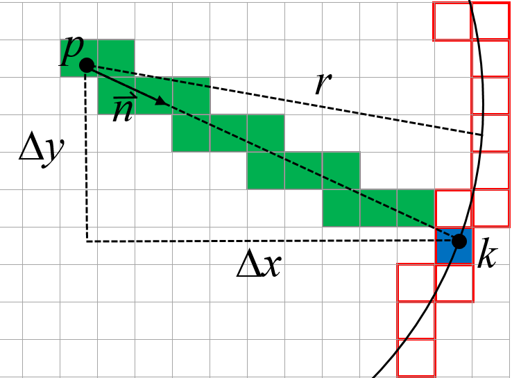
(a) Votes cast (in 2D) for offset, vector, and radial voting

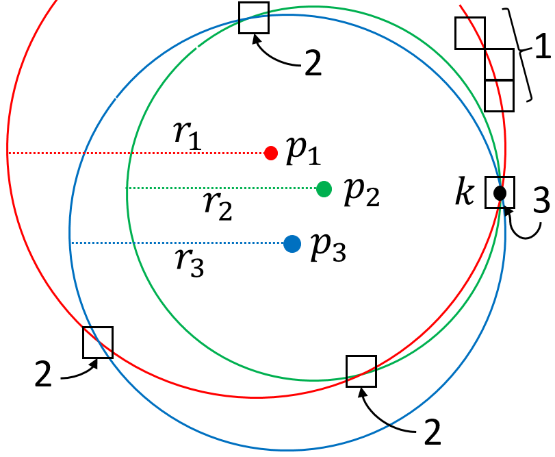
(b) Accumulator space values after radial voting for 3 points

Figure 2: Keypoint Voting Schemes in 2D: a) Pixel $p$ casts votes for keypoint $k$ at blue bin (offset and vector voting), green bins (vector voting), and red bins (radial voting). b) Radial votes cast for pixels $p_{1}$, $p_{2}$, and $p_{3}$ result in bin peaks at the intersection of the circles, with the peak occuring at keypoint $k$

3.1 Keypoint Voting Scheme Alternatives

The three keypoint voting schemes are illustrated in 2D in Fig. 2a, for image pixel $p$ and keypoint $k$ to be estimated. The grid represents the (initially empty) accumulator space bins, which are the voxel space elements where votes are cast. In offset voting, the values of $\Delta x$ and $\Delta y$ are estimated from forward inference through the network. These values are used to offset $p$ to reference that accumulator bin (shown in blue) containing $k$, the value of which is then incremented. Alternately, in vector voting, the direction $\vec{n}$ is estimated, and all bins (shown in green and blue) that intersect with $\vec{n}$ are incremented. Finally, in radial voting, the scalar $r$ is estimated, and all bins (shown outlined in red) are incremented that intersect with the perimeter of the circle of radius $r$ centered at $p$. When repeated for all image pixels, the bin containing $k$ will contain the maximum accumulator space value, irrespective of which scheme is used, so long as the quantities estimated by network inference are sufficiently accurate. In Fig. 2b, circles generated by radial voting are illustrated for three image pixels. Each bin contains a count of the number of circle perimeters that it intersects, such that the peak value of 3 indicates the location of keypoint $k$. The above three voting schemes extend directly to 3D space, in which the accumulator space is a grid of voxels, the offset scheme contains an additional $\Delta z$ component, $\vec{n}$ is a 3-dimensional vector, and the radial scheme casts votes on the surfaces of 3D spheres rather than 2D circles.

Formally, let $p_{i}$ be pixel from RGB-D image $I$ with 2D image coordinate $(u_{i},v_{i})$ and corresponding 3D camera frame coordinate $(x_{i},y_{i},z_{i})$. Further let $k^{\theta}_{j}\!=\!(x_{j},y_{j},z_{j})$ denote the camera frame coordinate of the $j^{th}$ keypoint of an object located at 6 DoF pose $\theta$. The quantity ${\bf m_{o}}$ regressed in the first offset scheme [18, 37] is the displacement between the two 3D points, denoted as ${\bf m_{o}}\!=\!(\Delta x,\Delta y,\Delta z)\!=\!(x_{i}\!-\!x_{j},\;y_{i}\!-\!y_{j},\;z_{i}\!-\!z_{j})$. Alternately, the 3D quantity ${\bf m_{v}}$ from the second vector scheme [36, 49] is the unit vector pointing to $k^{\theta}_{j}$ from $p_{i}$, denoted as ${\bf m_{v}}\!=\!(dx,dy,dz)\!=\!\frac{\bf m_{o}}{\lVert{\bf m_{o}}\rVert}$. The 3D vector scheme can alternately be parametrized into a 2D polar scheme, denoted as ${\bf m_{p}}\!=\!(\phi,\psi)\!=\!(\cos^{-1}{dz},\tan^{-1}\frac{dy}{dx})$. Finally, the 1D quantity ${\bf m_{r}}$ from the radial scheme proposed here is simply the Euclidean distance between the points, i.e. ${\bf m_{r}}\!=\!\lVert{\bf m_{o}}\rVert$.

The above quantities encode different information about the relationship between $p_{i}$ and $k^{\theta}_{j}$. For example, ${\bf m_{v}}$, ${\bf m_{p}}$, and ${\bf m_{r}}$ can be derived directly from ${\bf m_{o}}$, whereas ${\bf m_{o}}$ cannot be derived from the others. Also, ${\bf m_{r}}$ and ${\bf m_{v}}$ (and ${\bf m_{p}}$) are independent of one another. This difference in geometric information leads to their different dimensionality, and ultimately the greater accuracy of radial voting, as discussed in Sec. 4.4.

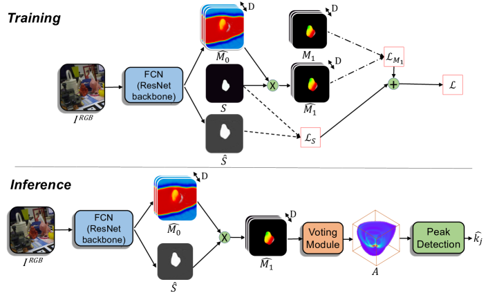
Figure 3: RCVPose training and inference. $\widehat{M}_{0}$, $\widehat{M}_{1}$, and $M_{1}$ have channel depth $D\!=\!1$ for radial, $D\!=\!2$ for polar, or $D\!=\!3$ for offset or vector voting schemes

3.2 Keypoint Estimation Pipeline

The above described voting schemes can be used interchangeably within a keypoint estimation pipeline. The training inputs (Fig. 3) are: RGB fields $I^{RGB}$ of image $I$; ground truth binary segmented image $S$ of the foreground object at pose $\theta$; ground truth keypoint coordinate $k^{\theta}_{j}$, and; the ground truth voting scheme values (i.e. one of ${\bf m_{o}}$, ${\bf m_{v}}$, ${\bf m_{p}}$ or ${\bf m_{r}}$) for each pixel in $S$, represented by matrix $M_{1}$. $M_{1}$ is calculated for a given $k^{\theta}_{j}$ using one of the voting scheme values, and has either channel depth $D\!=\!3$ for ${\bf m_{o}}$ or ${\bf m_{v}}$, $D\!=\!2$ for ${\bf m_{p}}$, or $D\!=\!1$ for ${\bf m_{r}}$. Both $S$ and $M_{1}$ are assessed to compute the loss $\mathcal{L}$ as:

$$\mathcal{L}=\mathcal{L}_{S}+\mathcal{L}_{M_{1}},$$ (1)

$$\mathcal{L}_{S}=\frac{1}{N}\sum_{i=1}^{N}\left|\widehat{S}_{i}-S_{i}\right|,$$ (2)

$$\mathcal{L}_{M_{1}}=\frac{1}{N}\sum_{i=1}^{N}\left(|\widehat{M_{1}}_{i}-{M_{1}}_{i}|\right),$$ (3)

with summations over all $N$ pixels. The network output is estimate $\widehat{S}$ of $S$, and (unsegmented) estimate $\widehat{M}_{0}$ of $M_{1}$.

At inference (Fig. 3), $I^{RGB}$ is fed to the network which returns estimates $\widehat{S}$ and $\widehat{M_{0}}$, the element-wise multiplication of which yields segmented estimate $\widehat{M}_{1}$. Each pixel $(u_{i},v_{i})$ of $\widehat{M}_{1}$, with corresponding 3D coordinate $(x_{i},y_{i},z_{i})$ drawn from the depth field $I^{D}$ of $I$, then independently casts a vote through the voting module into the initially empty 3D accumulator space $A$.

Vote casting is performed for each $(u_{i},v_{i})$, and is distinct for each voting scheme. In offset voting, accumulator space $A$ bin $A[x_{i}\!+\!\widehat{M}_{1}[u_{i},v_{i},0],\ y_{i}\!+\!\widehat{M}_{1}[u_{i},v_{i},1],z_{i}\!+\!\widehat{M}_{1}[u_{i},v_{i},2]]$ is incremented, thereby voting for the specific bin of $A$ that contains keypoint $k^{\theta}_{j}$. In vector and polar voting, every $A$ bin is incremented that intersects with the ray $\alpha(x_{i}\!+\!\widehat{M}_{1}[u_{i},v_{i},0],\ y_{i}\!+\!\widehat{M}_{1}[u_{i},v_{i},1],\ z_{i}\!+\!\widehat{M}_{1}[u_{i},v_{i},2])$, for $\alpha>0$, thereby casting a vote for every bin along the ray that intersects with $(x_{i},y_{i},z_{i})$ and $k^{\theta}_{j}$. Finally, in radial voting, every $A$ bin is incremented that intersects with the sphere of radius $\widehat{M}_{1}[u_{i},v_{i}]$ centered at $(x_{i},y_{i},z_{i})$, thereby voting for every bin that lies on the surface of a sphere upon which $k^{\theta}_{j}$ resides. Whichever scheme is used, at the conclusion of vote casting for all $(u_{i},v_{i})$, a global peak will exist in the $A$ bin containing $k^{\theta}_{j}$, and a simple peak detection operation is then sufficient to estimate keypoint position $\widehat{k}^{\theta}_{j}$, within the precision of $A$. The radial voting scheme has been shown to be more accurate than the other schemes at keypoint estimation, as shown in the experiments in Sec. 4.4.

3.3 RCVPose

The above keypoint voting method formed the core of RCVPose. Radial voting was used, based on its superior accuracy as demonstrated in Sec. 4.4. The network of Fig. 3 was used with ResNet-152 as the FCN-ResNet module. The minimal $K\!\!=\!3$ keypoints were used for each object, selected from the corners of each object’s bounding box. Based on Sec. 4.5, keypoints were scaled to lie beyond the surface of each object, $\sim 2$ object radius units from its centroid.

The network structure was based on a Fully Convolutional ResNet-152 [12], similar to PVNet [36], albeit with two main differences. First, we replaced LeakyReLU with ReLU as the activation function. This was because our radial voting scheme only includes positive values, in contrast to the vector voting scheme of PVNet which also admits negative values. Second, we increased the number of skip connections linking the downsampling and upsampling layers from three to five, to include extra local features when upsampling [24].

All voxels were initialized to zero, with their values incremented as votes were cast. The voting process is similar to 3D sphere rendering, wherein those voxels that intersect with the sphere surface have their values incremented. The process is based on Andre’s circle rendering algorithm [2]. We generate a series of 2D slices of $A$ parallel to the x-y plane, that fall within the sphere radius from the sphere center in both directions of the z-axis. For each slice, the radius of the circle formed by the intersection of the sphere and that slice is calculated, and all voxels that intersect with this circumference are incremented. The algorithm is accurate and efficient, requiring that only a small portion of the voxels be visited for each sphere rendering. It was implemented in Python and parallelized at the thread level, and executes with an efficiency similar to forward network inference.

Once the $K\!\!=\!3$ keypoint locations are estimated for an image, it is straightforward to determine the object’s 6 DoF rigid transformation $\theta$, from the corresponding estimated scene and ground truth object keypoint coordinates [17, 25]. This is analogous to the approach of [14], and is efficient compared to previous pure RGB approaches [36] which employ an iterative PnP method.

4 Experiments

4.1 Datasets

The LINEMOD dataset [15] includes $1200$ images per object. The training set contains only 180 training samples using the standard $15\%/85\%$ training/testing split [49, 36, 5, 14, 18]. We augmented the dataset by rendering the objects with a random rotation and translation, transposed using the BOP rendering kit [16] onto a background image drawn from the MSCOCO dataset [23]. An additional 1300 augmented images were generated for each object in this way, inflating the training set to 1480 images per object.

The LINEMOD depth images have an offset compared to the ground-truth pose values, for unknown reasons [28]. To reduce the impact of this offset, we regenerated the depth field for each training image from the ground truth pose, by reprojecting the depth value drawn from the object pose at each 2D pixel coordinate. The majority (1300) of the resulting training set were in this way purely synthetic images, and the minority (180) comprised real RGB and synthetic depth. All test images were original, real and unaltered.

Occlusion LINEMOD [3] is a re-annotation of LINEMOD comprising a subset of 1215 challenging test images of partially occluded objects. The protocol is to train using LINEMOD images only, and then test on Occlusion LINEMOD to verify robustness.

YCB-Video [49] is a much larger dataset, containing 130K key frames of 21 objects over 92 videos. We split 113K frames for training and 27K frames for testing, following PVN3D [14]. For data augmentation, YCB-Video provides 80K synthetic images with random object poses, rendered on a black background. We repeated here the process described above, by rendering random MSCOCO images as background. The complete training dataset therefore comprised 113K real + 80K synthetic = 193K images.

4.2 Implementation Details

Prior to training, each RGB image is shifted and scaled to adhere to the ImageNet mean and standard deviation [6]. The 3D coordinates were calculated from the image depth fields and represented in decimeter units, as all LINEMOD and YCB-Video objects are at most 1.5 decimeters in diameter and the backbone network can estimate better when the output is within a normalized range. The loss functions of Eqs. 1-3 were used with an Adam optimizer, with initial learning rate lr=1e-4. The lr was adjusted on a fixed schedule, re-scaled by a factor of $0.1$ every 70 epochs. The network trained for 300 and 500 epochs for each object in the LINEMOD and YCB-Video datasets respectively, with batch size 32.

The accumulator space $A$ is represented as a flat 3D integer array, i.e. an axis-aligned grid of voxel cubes. The size of $A$ was set for each test image to the bounding box of the 3D data. The voxel resolution was set to 5 mm, which was found to be a good tradeoff between memory expense and keypoint localization accuracy (see Supplementary Material Sec. S.4.5).

For each object, 3 instances of the network were trained, one for each keypoint. We also implemented a version in which all 3 keypoints were trained simultaneously, within a single network. In this version, the $\hat{M}_{0}$, $\hat{M}_{1}$, and $M_{1}$ representations of Fig. 3 are replicated 3 times, and the FCN-ResNet weights are shared. Our experiments (detailed in the supplementary material) showed that the accuracy was poorer for this version, than when using separate networks for each keypoint. The only two methods that have used a combined network for all keypoints and all objects are GDRNet [48] and SOPose [7], against which our performance compares favourably (see Sec. 4.6).

4.3 Evaluation Metrics

We follow the ADD(s) metric defined by [15] to evaluate LINEMOD, whereas YCB-Video is evaluated based on both ADD(s) and AUC as proposed by [49]. All metrics are based on the distances between corresponding points as objects are transformed by the ground truth and estimated transformations. ADD measures the average distance between corresponding points, whereas ADDs averages the minimum distance between closest points, and is more forgiving for symmetric objects. A pose is considered correct if its ADD(s) falls within 10$\%$ of the object radius. AUC applies the ADD(s) values to determine the success of an estimated transformation, integrating these results over a varying 0 to 100 mm threshold.

4.4 Comparison of Keypoint Voting Schemes

We first conducted an experiment to evaluate the relative accuracies of the four voting schemes at keypoint localization, using the process from Sec. 3.2. Each scheme used the same $15\%/85\%$ train/test split of a subset of objects from the LINEMOD dataset. All four schemes used the exact same backbone network and hyperparameters. Specifically, they all used a fully convolutional ResNet-18 [24], batch size 48, initial learning rate 1e-3, and Adam optimizer, with accumulator space resolution of 1 mm. They were all trained with a fixed learning rate reduction schedule, which reduced the rate by a factor of 10 following every 70 epochs, and all trials trained until they fully converged.

Table 1: Keypoint localization error $\bar{\epsilon}$, for surface (FPS) and disperse keypoints: mean $\mu$ and standard deviation $\sigma$ for 4 voting schemes $\{v,o,p,r\}$, with $\bar{r}$ = mean keypoint distance to object centroid

			$\bar{\epsilon}$ [mm]
			vector (3D)		offset (3D)		polar (2D)		radial (1D)
		$\bar{r}$ [mm]	$\mu_{v}$	$\sigma_{v}$	$\mu_{o}$	$\sigma_{o}$	$\mu_{p}$	$\sigma_{p}$	$\mu_{r}$	$\sigma_{r}$
ape	FPS	61.2	10.0	5.8	5.8	2.6	5.6	2.4	1.3	0.7
driller		129.4	10.0	2.3	6.5	4.7	5.3	2.5	2.2	1.0
eggbox		82.5	11.8	5.3	5.2	2.7	4.9	1.9	2.0	0.7
ape	disperse	142.1	12.5	7.6	10.4	5.3	5.7	2.5	1.8	0.8
driller		318.8	11.3	8.2	9.5	3.5	5.2	2.6	2.7	0.8
eggbox		197.3	13.7	8.5	11.4	4.7	7.2	3.4	2.4	1.2

The only difference between trials, other than the selective use of either ${\bf m_{o},m_{v},m_{p}}$ or ${\bf m_{r}}$ in training $\widehat{M}_{1}$, was a slight variation in the loss functions. For ${\bf m_{o}}$ and ${\bf m_{r}}$, the L1 loss from Eqs. 1-3 was used, identical to the offset voting in PVN3D [14]. Alternately, for ${\bf m_{v}}$ and ${\bf m_{p}}$, the Smooth L1 equivalents of Eqs. 2 and 3 (with $\beta\!\!=\!\!1$) were used, as in PVNet [36] (albeit therein using a 2D accumulator space).

Surface Keypoints:

Sets of size $K$= 4 surface keypoints were selected for each object tested, using the Farthest Point Sampling (FPS) method [9]. FPS selects points on the surface of an object which are well separated, and is a popular keypoint generation strategy [36, 14, 38, 37]. Following training, each keypoint’s location $\widehat{k}_{j}^{\theta_{i}}$ was estimated by passing each test image $I_{i}$ through the network, as in Fig. 3. The error $\epsilon_{i,j}$ for each estimate was its Euclidean distance from its ground truth location, i.e. $\epsilon_{i,j}\!=\!\lVert\widehat{k}_{j}^{\theta_{i}}\!-\!k_{j}^{\theta_{i}}\rVert$. The average of $\epsilon_{i,j}$ for an object over all test images and keypoints was the keypoint estimation error, denoted as $\bar{\epsilon}$.

Each voting scheme was implemented with care, so that they were numerically accurate and equivalent. To test the correctness of voting in isolation, ground truth values of $M_{1}$ calculated for each object and voting scheme were passed directly into the voting module, effectively replacing $\widehat{M}_{1}$ with $M_{1}$ in the inference stage of Fig. 3. For each voting scheme, the average $\bar{\epsilon}$ for all objects was similar and less than the accumulator space resolution of 1 mm, indicating that the implementations were correct and accurate.

The $\bar{\epsilon}$ values were evaluated for the four voting schemes for the ape, driller and eggbox LINEMOD objects as summarized in Table 1. These three particular objects were chosen as the ape is the smallest and the driller the largest of the objects, whereas the eggbox includes a rotational symmetry. Table 1 includes a measure of the average distance $\bar{r}$ of the ground truth keypoints to each object centroid. Radial voting is seen to be the most accurate method, with a mean value 1.9-4.3x more accurate than the next most accurate polar voting, with smaller standard deviations. Notably, the ordinal relationship between the four schemes remains consistent across the scheme dimensionality, which indicates that dimensionality impacts keypoint localization error.

Disperse Keypoints:

We repeated this experiment for keypoints selected from the corners of each object’s bounding box, which was first scaled by a factor of 2 so that the keypoints were dispersed to fall outside of the object’s surface. The results in Table 1 indicate that radial voting still outperforms the other two schemes by a large margin. Whereas the other two methods decrease in accuracy sharply as the mean keypoint distance $\bar{r}$ increases, radial voting accuracy degrades more gracefully. For example, for the ape, the 232$\%$ increase in $\bar{r}$ from 61.2 to 142.1 mm, reduced accuracy for offset voting by $80\%$ (from 5.8 to 10.4 mm), but only by $23\%$ (from 2.2 to 2.7 mm) for radial voting.

The improved accuracy of radial voting is likely due to the fact that the radial scheme regresses a 1D quantity, compared with the 2D polar, and the 3D offset and vector scheme quantities. It seems likely that the errors in each independent dimension compound during voting. This is further supported by the recognition that the polar scheme is simply a reduced dimensionality parametrization of the vector scheme, and yet its performance is far superior, with between 1.7-2.4x greater accuracy. Radial voting also has a degree of resilience to rotations, which is lacking in the other schemes. Specifically, the three voting quantities ${\bf m_{o}}$, ${\bf m_{v}}$, and ${\bf m_{p}}$ are all sensitive to object in-plane rotations, whereas only radius scheme ${\bf m_{r}}$ is invariant to in-plane rotations.

4.5 Keypoint Dispersion

4.5.1 Impact on Transformation Estimation:

It was suggested in [36] that 6 DoF pose estimation accuracy is improved by selecting keypoints that lie on the object surface, rather than the bounding box corners which lie just beyond the object surface. This may be the case when keypoint localization error increases signficantly with keypoint disperson, as occurs with vector and offset voting. There is, however, an advantage to dispersing the keypoints farther apart when using radial voting, which has a lower estimation error.

To demonstrate this, we conducted an experiment in which the keypoint locations were dispersed to varying degrees under a constant keypoint estimation error, with the impact measured on the accuracy of the resulting estimated transformation. We first selected a set $\cal{K}$=$\{k_{j}\}_{j=1}^{4}$ keypoints on the surface of an object, using the FPS strategy. This set was then rigidly transformed by $T$, comprising a random rotation (within $0^{\circ}$ to $360^{\circ}$ for each axis) and a random translation (within 1/2 of the object radius), to form keypoint set ${\cal{K}}_{T}$. Each keypoint in ${\cal{K}}_{T}$ was then independently pertubed by a magnitude of 1.5 mm in a random direction, to simulate the keypoint estimation error of the radial voting scheme, resulting in (estimated) keypoint set $\widetilde{\cal{K}}_{\widetilde{T}}$.

Next, the estimated transformation $\widetilde{T}$ between $\widetilde{\cal{K}}_{\widetilde{T}}$ and the original (ground truth) keypoint set $\cal{K}$ was calculated using the Horn method [17]. This process simulates the pose estimation that would occur between estimated keypoint locations, each with some error, and their corresponding ground truth model keypoints. The surface points of the object were then transformed by both the ground truth $T$ and the estimated $\widetilde{T}$ transformations, and the distances separating corresponding transformed surface points were compared, as a measure of the accuracy of the estimated transformation.

The above process was repeated for versions of $\cal{K}$ that were dispersed by scaling an integral factor of the object radius from the object centroid. The exact same error perturbations (i.e. magnitudes and directions) were applied to each keypoint for each new scale value. The scaled trials therefore represented keypoints that were dispersed more distant from the object centroid, albeit with the exact same localization error.

This process was executed for all Occlusion LINEMOD objects, with 100 trials for each scale factor value from 1 to 5. The means of the corresponding point distances (i.e. the ADD metric as defined in [15]) are plotted in Fig. 4(a). It can be seen that ADD decreases for the first few scale factor increments for all objects, indicating an improved transformation estimation accuracy for larger keypoint dispersions. This increase in accuracy stems from improved rotational estimates, as the same positional perturbation error of a keypoint under a larger moment arm will result in a smaller angular error. The translational component of the transformation is not impacted by the scaling, as the Horn method starts by centering the two point clouds. After a certain increase in scale factor of 3 or 4, the unaffected translational error dominates, and the error plateaus.

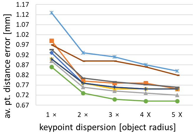
(a) Transformation error ($\downarrow$)

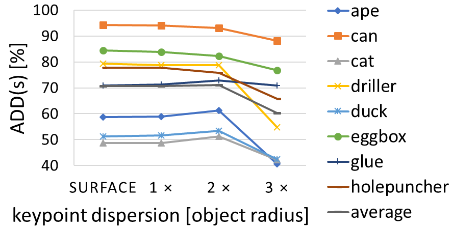
(b) 6 DoF pose ADD(s) ($\uparrow$)

Figure 4: Impact of keypoint dispersion on (a) Transformation estimation error, and (b) 6 DoF pose estimation ADD(s)

This experiment shows that the transformation estimate from corresponding ground truth and estimated keypoints will be more accurate, when the keypoints are dispersed further ($\sim\!\!1$ object radius, i.e. a scale of 2x) from the object’s surface, when keypoint estimation error itself remains small ($\sim\!\!1.5$ cm).

4.5.2 Impact on 6 DoF Pose Estimation:

The above result can be leveraged to further improve the accuracy of 6 DoF pose estimation when using radial voting. An experiment was executed for all Occlusion LINEMOD objects for varying keypoint dispersions. The keypoints were first selected to lie on the surface of each object using FPS, and the complete RCVPose inference pipeline was executed, yielding an ADD(s) value for each trial image. The keypoints were then projected outward from each object’s centroid to a distance of 1, 2 and 3 object radius values, and RCVPose inference was once again executed and ADD(s) recalculated.

The results are plotted in Fig. 4(b). Of the 8 objects, 4 had a higher ADD(s) value at a dispersion of 2x, as did the average over all objects. It seems that the decreased transformation estimation error (Fig. 4(a)) at 2x radius dispersion more than compensates for the gradual increase in keypoint localization error exhibited by radial voting.

Table 2: LINEMOD and Occlusion
LINEMOD accuracy results

		ADD(s) [$\%$]
Mode	Method	LM	O-LM
	SSD6D [19]	9.1	-
	Oberweger [31]	-	27.1
	Hu et al. [18]	-	30.4
	Pix2Pose [33]	72.4	32.0
	DPOD [50]	83.0	32.8
	PVNet [36]	86.3	40.8
RGB	DeepIM [22]	88.6	-
	PPRN [44]	93.9	58.4
	GDR-Net [48]	93.7	62.2
	SO-Pose [7]	96.0	62.3
	YOLO6D [43]	56.0	6.4
	SSD6D+ref [19]	34.1	27.5
RGB	PoseCNN [49]	-	24.9
+D ref	DPOD+ref [50]	95.2	47.3
	DenseFusion [46]	94.3	-
	PVN3D [14]	99.4	63.2
	PR-GCN [51]	99.6	65.0
	FFB6D [13]	99.7	66.2
	RCVPose	99.4	70.2
RGB-D	RCVPose+ICP	99.7	71.1

Table 3: YCB-Video accuracy results

D ref?	Method	ADD(s)	AUC
	PoseCNN [49]	59.9	75.8
	DF (per-pixel) [46]	82.9	91.2
	SO-Pose [7]	56.8	90.9
	GDR-Net [48]	60.1	91.6
	PVN3D [14]	91.8	95.5
	PR-GCN [51]	-	95.8
	FFB6D [13]	92.7	96.6
No	RCVPose	95.2	96.6
	PoseCNN [49]	85.4	93.0
	DF (iterative) [46]	86.1	93.2
	PVN3D [14]+ICP	92.3	96.1
	FFB6D [13]+ICP	93.1	97.0
Yes	RCVPose+ICP	95.9	97.2

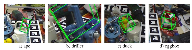
Figure 5: RCVPose sample Occlusion LINEMOD results: Blue box = ground truth, green box = estimate. RCVPose shows robustness to (even severe) occlusion

4.6 Comparison with SOTA

We next compared RCVPose against other recent competitive methods in the literature. We achieved state-of-art results on all three datasets, under a moderate training effort (i.e. hyper-parameter adjustment). The most challenging dataset was Occlusion LINEMOD, with results in Table 3. RCVPose+ICP outperformed all other methods on average, achieving $71.1\%$ mean accuracy, exceeding the next closest method PVN3D by $7.9\%$. It achieved the top performance on all objects except duck, where PVNet had the best result. Even without ICP refinement, RCVPose achieved close to the same results at $70.2\%$ mean accuracy.

One strength of RCVPose is scale tolerance. Unlike most other methods whose performance reduced with smaller objects, our method was not impacted much. Significantly, accuracy improved over FFB6D from $47.2\%$, $45.7\%$ to $61.3\%$, $51.2\%$ for the ape and cat, respectively. Another advantage is that it accumulates votes independently for each pixel and is therefore robust to partial occlusions, capable of recognizing objects that undergo up to $70\%$ occlusion (see Fig. 5). The LINEMOD dataset is less challenging, as objects are unoccluded. As listed in Table 3, RCVPose+ICP still achieved the highest mean accuracy of $99.7\%$, slightly exceeding the tie between RCVPose (without ICP) and PVN3D. RCVPose+ICP was the only method to achieve $100\%$ accuracy for more than one object. Again the RGB-D methods outperformed all other data modes, and the top RGB method that included depth refinement [33] outperformed the best pure RGB method [27], supporting the benefits of the added depth mode.

The YCB-Video results in Table 3 list AUC and ADD(s), with and without depth refinement. RCVPose is the top performing method, achieving from $95.2\%$ to $95.9\%$ ADD(s) and from $96.6\%$ to $97.2\%$ AUC accuracy, outperforming the next best method FFB6D by $2.8\%$ ADD(s) and $0.2\%$ AUC. Notably, RCVPose increased ADD(s) of the relatively small tuna fish can by a full $6\%$ compared to the second best PVN3D. We also evaluated RCVPose on the BOP challenge benchmark [16], which is a standardized split of a number of datasets. Our results on their LINEMOD, Occlusion LINEMOD, and YCB-Video splits showed that RCVPose outperformed all other published results tested on this benchmark, when averaged over all 3 datasets (see Supplementary Material Sec. S.3). RCVPose runs at 18 fps on a server with an Intel Xeon 2.3 GHz CPU and RTX8000 GPU for a $640\!\times\!480$ image input. This compares well to other voting-based methods, such as PVNet at 25 fps, and PVN3D at 5 fps. The backbone network forward path, radial voting process, and Horn transformation solver take approximately 10, 41, and 4 msecs. per image respectively at inference time.

5 Conclusion

We have proposed RCVPose, a hybrid 6 DoF pose estimator with a ResNet-based radial estimator and a novel keypoint radial voting scheme. Our radial voting scheme is shown to be more accurate than previous schemes, especially when the keypoints are more dispersed, which leads to more accurate pose estimation requiring only 3 keypoints. We achieved state-of-the-art results on three popular benchmark datasets, YCB-Video, LINEMOD and the challenging Occlusion LINEMOD, ranking high on the BOP Benchmark, with an 18 fps runtime. A limitation is that training and inference are executed separately for each object and keypoint (also true for other recent competitive approaches) and that the 3D voting space is memory intensive, which will be the focus of future work.

Acknowledgements:

Thanks to Bluewrist Inc. and NSERC for their support of this work.

References

- [1] Aiger, D., Mitra, N.J., Cohen-Or, D.: 4-points congruent sets for robust surface registration. ACM Transactions on Graphics 27(3), #85, 1–10 (2008)
- [2] Andres, E.: Discrete circles, rings and spheres. Computers & Graphics 18(5), 695–706 (1994)
- [3] Brachmann, E., Krull, A., Michel, F., Gumhold, S., Shotton, J., Rother, C.: Learning 6d object pose estimation using 3d object coordinates. In: European conference on computer vision. pp. 536–551. Springer (2014)
- [4] Brogan, J., Bharati, A., Moreira, D., Rocha, A., Bowyer, K.W., Flynn, P.J., Scheirer, W.J.: Fast local spatial verification for feature-agnostic large-scale image retrieval. IEEE Transactions on Image Processing 30, 6892–6905 (2021)
- [5] Bukschat, Y., Vetter, M.: Efficientpose–an efficient, accurate and scalable end-to-end 6d multi object pose estimation approach. arXiv preprint arXiv:2011.04307 (2020)
- [6] Deng, J., Dong, W., Socher, R., Li, L., Kai Li, Li Fei-Fei: Imagenet: A large-scale hierarchical image database. In: 2009 IEEE Conference on Computer Vision and Pattern Recognition. pp. 248–255 (2009). https://doi.org/10.1109/CVPR.2009.5206848
- [7] Di, Y., Manhardt, F., Wang, G., Ji, X., Navab, N., Tombari, F.: So-pose: Exploiting self-occlusion for direct 6d pose estimation. In: Proceedings of the IEEE/CVF International Conference on Computer Vision. pp. 12396–12405 (2021)
- [8] Duda, R.O., Hart, P.E.: Use of the hough transformation to detect lines and curves in pictures. Communications of the ACM 15(1), 11–15 (1972)
- [9] Eldar, Y., Lindenbaum, M., Porat, M., Zeevi, Y.Y.: The farthest point strategy for progressive image sampling. IEEE Transactions on Image Processing 6(9), 1305–1315 (1997)
- [10] Fischler, M.A., Bolles, R.C.: Random sample consensus: a paradigm for model fitting with applications to image analysis and automated cartography. Communications of the ACM 24(6), 381–395 (1981)
- [11] Gall, J., Yao, A., Razavi, N., Van Gool, L., Lempitsky, V.: Hough forests for object detection, tracking, and action recognition. IEEE Transactions on Pattern Analysis and Machine Intelligence 33(11), 2188–2202 (2011). https://doi.org/10.1109/TPAMI.2011.70
- [12] He, K., Zhang, X., Ren, S., Sun, J.: Deep residual learning for image recognition. In: Proceedings of the IEEE conference on computer vision and pattern recognition. pp. 770–778 (2016)
- [13] He, Y., Huang, H., Fan, H., Chen, Q., Sun, J.: Ffb6d: A full flow bidirectional fusion network for 6d pose estimation. In: Proceedings of the IEEE/CVF Conference on Computer Vision and Pattern Recognition. pp. 3003–3013 (2021)
- [14] He, Y., Sun, W., Huang, H., Liu, J., Fan, H., Sun, J.: Pvn3d: A deep point-wise 3d keypoints voting network for 6dof pose estimation. In: Proceedings of the IEEE/CVF Conference on Computer Vision and Pattern Recognition (CVPR) (June 2020)
- [15] Hinterstoisser, S., Lepetit, V., Ilic, S., Holzer, S., Bradski, G., Konolige, K., Navab, N.: Model based training, detection and pose estimation of texture-less 3d objects in heavily cluttered scenes. In: Asian conference on computer vision. pp. 548–562. Springer (2012)
- [16] Hodaň, T., Sundermeyer, M., Drost, B., Labbé, Y., Brachmann, E., Michel, F., Rother, C., Matas, J.: Bop challenge 2020 on 6d object localization. In: European Conference on Computer Vision. pp. 577–594. Springer (2020)
- [17] Horn, B.K.P., Hilden, H.M., Negahdaripour, S.: Closed-form solution of absolute orientation using orthonormal matrices. J. Opt. Soc. Am. A 5(7), 1127–1135 (Jul 1988). https://doi.org/10.1364/JOSAA.5.001127, http://josaa.osa.org/abstract.cfm?URI=josaa-5-7-1127
- [18] Hu, Y., Hugonot, J., Fua, P., Salzmann, M.: Segmentation-driven 6d object pose estimation. In: Proceedings of the IEEE/CVF Conference on Computer Vision and Pattern Recognition. pp. 3385–3394 (2019)
- [19] Kehl, W., Manhardt, F., Tombari, F., Ilic, S., Navab, N.: Ssd-6d: Making rgb-based 3d detection and 6d pose estimation great again. In: Proceedings of the IEEE international conference on computer vision. pp. 1521–1529 (2017)
- [20] Labbé, Y., Carpentier, J., Aubry, M., Sivic, J.: Cosypose: Consistent multi-view multi-object 6d pose estimation. In: European Conference on Computer Vision. pp. 574–591. Springer (2020)
- [21] Lamdan, Y., Wolfson, H.J.: Geometric hashing: A general and efficient model-based recognition scheme. In: [1988 Proceedings] Second International Conference on Computer Vision. pp. 238–249 (1988). https://doi.org/10.1109/CCV.1988.589995
- [22] Li, Y., Wang, G., Ji, X., Xiang, Y., Fox, D.: Deepim: Deep iterative matching for 6d pose estimation. In: Proceedings of the European Conference on Computer Vision (ECCV). pp. 683–698 (2018)
- [23] Lin, T.Y., Maire, M., Belongie, S., Hays, J., Perona, P., Ramanan, D., Dollár, P., Zitnick, C.L.: Microsoft coco: Common objects in context. In: European conference on computer vision. pp. 740–755. Springer (2014)
- [24] Long, J., Shelhamer, E., Darrell, T.: Fully convolutional networks for semantic segmentation. In: Proceedings of the IEEE conference on computer vision and pattern recognition. pp. 3431–3440 (2015)
- [25] Lorusso, A., Eggert, D.W., Fisher, R.B.: A comparison of four algorithms for estimating 3-D rigid transformations. Citeseer (1995)
- [26] Lowe, D.G.: Object recognition from local scale-invariant features. In: Proceedings of the seventh IEEE international conference on computer vision. vol. 2, pp. 1150–1157. Ieee (1999)
- [27] Manhardt, F., Arroyo, D.M., Rupprecht, C., Busam, B., Birdal, T., Navab, N., Tombari, F.: Explaining the ambiguity of object detection and 6d pose from visual data. In: Proceedings of the IEEE/CVF International Conference on Computer Vision (ICCV) (October 2019)
- [28] Manhardt, F., Kehl, W., Navab, N., Tombari, F.: Deep model-based 6d pose refinement in rgb. In: Proceedings of the European Conference on Computer Vision (ECCV). pp. 800–815 (2018)
- [29] Mohamad, M., Ahmed, M.T., Rappaport, D., Greenspan, M.: Super generalized 4pcs for 3d registration. In: 2015 International Conference on 3D Vision. pp. 598–606 (2015). https://doi.org/10.1109/3DV.2015.74
- [30] Mohamad, M., Rappaport, D., Greenspan, M.: Generalized 4-points congruent sets for 3d registration. In: 2014 2nd International Conference on 3D Vision. vol. 1, pp. 83–90 (2014). https://doi.org/10.1109/3DV.2014.21
- [31] Oberweger, M., Rad, M., Lepetit, V.: Making deep heatmaps robust to partial occlusions for 3d object pose estimation. In: Proceedings of the European Conference on Computer Vision (ECCV). pp. 119–134 (2018)
- [32] Olson, C.F.: Efficient pose clustering using a randomized algorithm (1997)
- [33] Park, K., Patten, T., Vincze, M.: Pix2pose: Pixel-wise coordinate regression of objects for 6d pose estimation. In: Proceedings of the IEEE/CVF International Conference on Computer Vision. pp. 7668–7677 (2019)
- [34] Park, K., Patten, T., Vincze, M.: Neural object learning for 6d pose estimation using a few cluttered images. In: Vedaldi, A., Bischof, H., Brox, T., Frahm, J.M. (eds.) Computer Vision – ECCV 2020. pp. 656–673. Springer International Publishing, Cham (2020)
- [35] Pavlakos, G., Zhou, X., Chan, A., Derpanis, K.G., Daniilidis, K.: 6-dof object pose from semantic keypoints. In: 2017 IEEE international conference on robotics and automation (ICRA). pp. 2011–2018. IEEE (2017)
- [36] Peng, S., Liu, Y., Huang, Q., Zhou, X., Bao, H.: Pvnet: Pixel-wise voting network for 6dof pose estimation. In: Proceedings of the IEEE/CVF Conference on Computer Vision and Pattern Recognition. pp. 4561–4570 (2019)
- [37] Qi, C.R., Litany, O., He, K., Guibas, L.J.: Deep hough voting for 3d object detection in point clouds. In: Proceedings of the IEEE/CVF International Conference on Computer Vision (ICCV) (October 2019)
- [38] Qi, C.R., Yi, L., Su, H., Guibas, L.J.: Pointnet++: Deep hierarchical feature learning on point sets in a metric space. arXiv preprint arXiv:1706.02413 (2017)
- [39] Redmon, J., Farhadi, A.: Yolov3: An incremental improvement. arXiv preprint arXiv:1804.02767 (2018)
- [40] Rothganger, F., Lazebnik, S., Schmid, C., Ponce, J.: 3d object modeling and recognition using local affine-invariant image descriptors and multi-view spatial constraints. International journal of computer vision 66(3), 231–259 (2006)
- [41] Schönberger, J.L., Price, T., Sattler, T., Frahm, J.M., Pollefeys, M.: A vote-and-verify strategy for fast spatial verification in image retrieval. In: Asian Conference on Computer Vision. pp. 321–337. Springer (2016)
- [42] Shao, J., Jiang, Y., Wang, G., Li, Z., Ji, X.: Pfrl: Pose-free reinforcement learning for 6d pose estimation. In: IEEE/CVF Conference on Computer Vision and Pattern Recognition (CVPR) (June 2020)
- [43] Tekin, B., Sinha, S.N., Fua, P.: Real-time seamless single shot 6d object pose prediction. In: Proceedings of the IEEE Conference on Computer Vision and Pattern Recognition. pp. 292–301 (2018)
- [44] Trabelsi, A., Chaabane, M., Blanchard, N., Beveridge, R.: A pose proposal and refinement network for better 6d object pose estimation. In: Proceedings of the IEEE/CVF Winter Conference on Applications of Computer Vision. pp. 2382–2391 (2021)
- [45] Tremblay, J., To, T., Sundaralingam, B., Xiang, Y., Fox, D., Birchfield, S.: Deep object pose estimation for semantic robotic grasping of household objects. arXiv preprint arXiv:1809.10790 (2018)
- [46] Wang, C., Xu, D., Zhu, Y., Martín-Martín, R., Lu, C., Fei-Fei, L., Savarese, S.: Densefusion: 6d object pose estimation by iterative dense fusion. In: Proceedings of the IEEE/CVF Conference on Computer Vision and Pattern Recognition. pp. 3343–3352 (2019)
- [47] Wang, G., Manhardt, F., Shao, J., Ji, X., Navab, N., Tombari, F.: Self6d: Self-supervised monocular 6d object pose estimation. In: European Conference on Computer Vision. pp. 108–125. Springer (2020)
- [48] Wang, G., Manhardt, F., Tombari, F., Ji, X.: Gdr-net: Geometry-guided direct regression network for monocular 6d object pose estimation. In: Proceedings of the IEEE/CVF Conference on Computer Vision and Pattern Recognition. pp. 16611–16621 (2021)
- [49] Xiang, Y., Schmidt, T., Narayanan, V., Fox, D.: Posecnn: A convolutional neural network for 6d object pose estimation in cluttered scenes (2018)
- [50] Zakharov, S., Shugurov, I., Ilic, S.: Dpod: 6d pose object detector and refiner. In: Proceedings of the IEEE/CVF International Conference on Computer Vision. pp. 1941–1950 (2019)
- [51] Zhou, G., Wang, H., Chen, J., Huang, D.: Pr-gcn: A deep graph convolutional network with point refinement for 6d pose estimation. In: Proceedings of the IEEE/CVF International Conference on Computer Vision. pp. 2793–2802 (2021)