Trigonometric multiplicative chaos and Application to random distributions

Abstract.

The random trigonometric series $\sum_{n=1}^{\infty}\rho_{n}\cos(nt+\omega_{n})$ on the circle $\mathbb{T}$ are studied under the conditions $\sum|\rho_{n}|^{2}=\infty$ and $\rho_{n}\to 0$, where $\{\omega_{n}\}$ are iid and uniformly distributed on $\mathbb{T}$. They are almost surely not Fourier-Stieljes series but define pseudo-functions. This leads us to develop the theory of trigonometric multiplicative chaos, which produces a class of random measures. The behaviors of the partial sums of the above series are proved to be multifractal. Our theory holds on the torus $\mathbb{T}^{d}$ of dimension $d\geq 1$.

Keywords– Multiplicative chaos, Random Fourier series, Hausdorff dimension, Riesz potential

MSC(2020)– 60G57, 60G46, 42A20,28A78

1. Introduction

Let us consider a random trigonometric series

(1.1) $$\sum_{n=1}^{\infty}X_{n}\cos(nt+\Phi_{n})$$

where the random complex variables $A_{n}:=X_{n}e^{i\Phi_{n}}$ ($X_{n},\Phi_{n}$ being real) are supposed to be independent and symmetric. It is the real part of the random Taylor trigonometric series

(1.2) $$\sum_{n=1}^{\infty}A_{n}e^{int}.$$

These series are well studied in [56] and [34] (see also [35]) under the condition $\mathbb{E}X_{n}^{4}\leq C(\mathbb{E}X_{n}^{2})^{2}$. If $\sum\mathbb{E}(X_{n}^{2})=+\infty$, the series (1.1) diverges almost surely almost everywhere and is almost surely not a Fourier-Stieltjes series (cf. [35], p. 54). Regular and irregular properties of the function defined by the series (1.1) are studied under the condition $\sum\mathbb{E}(X_{n}^{2})<+\infty$ (cf. [35], [50]).

We would like to study the series (1.1) under the following assumptions

(1.3) $$\sum_{n=1}^{\infty}\mathbb{E}X_{n}^{2}\ =\infty,\qquad\sum_{n=1}^{\infty}\mathbb{E}X_{n}^{4}\ <\infty.$$

One of our objects of study is the behaviors of the partial sums of the pseudo function defined by the series (1.1):

(1.4) $$S_{N}(t):=S_{N}(t,\omega):=\sum_{n=1}^{N}X_{n}\cos(nt+\Phi_{n}).$$

We also assume that $\{\Phi_{n}\}$ are independent and uniformly distributed on the circle $\mathbb{T}:=\mathbb{R}/2\pi\mathbb{R}$ which is identified with the interval $[0,2\pi)$ and that $\{X_{n}\}$ are independent quasi-gaussian and independent of $\{\Phi_{n}\}$. A real random variable $X$ is said to be quasi-gaussian if $\mathbb{E}(X^{2m})=O(K^{m}m!)$ for some $K\geq 0$. Recall that $X$ is said to be subgaussian if $\mathbb{E}e^{\lambda X}\leq e^{\frac{1}{2}\tau^{2}\lambda^{2}}$ for some $\tau>0$ and all $\lambda\in\mathbb{R}$. We know that $X$ is subgaussian if and only if it is centered and quasi-gaussian ([35], p. 82). As we shall prove, the behavior of $S_{N}(t)$ is very multifractal, meaning that for uncountably many functions $L:\mathbb{N}\to\mathbb{R}$ of different orders, the sets $\{t:S_{N}(t)\sim L(N)\}$ have positive Hausdorff dimensions.

The partial sum $S_{N}$ is a stationary process on $\mathbb{T}$ with its correlation function equal to $\mathbb{E}S_{N}(t)S_{N}(s)=H_{N}(t-s),$ where

$$H_{N}(t)=\frac{1}{2}\sum_{n=1}^{N}\mathbb{E}X_{n}^{2}\cos nt.$$

The limit $H(t):=\lim_{N\to\infty}H_{N}(t)$, if exists, is defined to be the correlation function of the series (1.1). In many cases, the correlation function

$$H(t)=\frac{1}{2}\sum_{n=1}^{\infty}\mathbb{E}X_{n}^{2}\cos nt$$

is well defined, integrable on $\mathbb{T}$ and continuous everywhere except $t=0$ (cf. Section 3). The correlation function $H$ will play an important role in the study of the series (1.1).

When $\mathbb{E}X_{n}^{2}=\frac{\alpha^{2}}{n}$, we get a special correlation function

$$H_{\alpha}(t)=\frac{\alpha^{2}}{2}\sum_{n=1}^{\infty}\frac{\cos nt}{n}=-\frac{\alpha^{2}}{2}\log\left(2\left|\sin\frac{t}{2}\right|\right).$$

Its exponential is the $\frac{\alpha^{2}}{2}$-order Riesz kernel

$$e^{H_{\alpha}(t)}\asymp\frac{1}{\left|\sin\frac{t}{2}\right|^{\frac{\alpha^{2}}{2}}}.$$

An effective tool that we shall use to study the series (1.1) is a class of the multiplicative chaotic measures, which are formally defined by

(1.5) $$\mu_{\omega}=\prod_{n=1}^{\infty}\exp\left(X_{n}\cos(nt+\Phi_{n})-\log\mathbb{E}I_{0}(X_{n})\right)dt,$$

where $I_{0}$ is the modified Bessel function of first order:

$$I_{0}(\alpha)=\int_{0}^{2\pi}e^{\alpha\sin x}\frac{dx}{2\pi}\qquad(\alpha\in\mathbb{R}).$$

More precisely, $\mu_{\omega}$ is the weak limit of the partial products of the infinite product in (1.5). These partial products form a non-negative martingale for each fixed $t$, which ensures the existence of the limit. We shall find conditions ensuring the non nullity of the measure $\mu_{\omega}$. A simple such condition is

(1.6) $$\int\int e^{H(t-s)}dtds<\infty$$

(cf. Proposition 4.1). Under the energy condition (1.6), we can define a probability measure $\mathcal{Q}$ on the product space $\mathbb{T}\times\Omega$ by the equality

$$\mathbb{E}_{\mathcal{Q}}h(t,\omega)=\mathbb{E}\int_{0}^{2\pi}h(t,\omega)d\mu_{\omega}(t)$$

holding for all bounded functions $h$. This measure is called Peyrière measure. An important fact is that “$\mathcal{Q}$-almost surely” means “almost surely (with respect to $P$) $\mu_{\omega}$-almost everywhere”. Another important fact is that the random variables $\{X_{n}\cos(nt+\Phi_{n})\}$ defined on $\mathbb{T}\times\Omega$ are $\mathcal{Q}$-independent (cf. Theorem 2.5). On the other hand, the measure $\mu_{\omega}$, through the measure $\mathcal{Q}$, well captures the points $t$ for which the series (1.1) has a specific property. In the definition of $\mu_{\omega}$ we can replace $\{X_{n}\}$ by $\{\alpha X_{n}\}$ to give a measure $\mu_{\omega,\alpha}$. So, we possess many measures as tools.

For the typical case $X_{n}=\frac{1}{\sqrt{n}}$, we shall prove that $\mu_{\omega,\alpha}=0$ almost surely if $|\alpha|>2$ (cf. Theorem 5.2). However, for $|\alpha|<2$ the Hausdorff dimension of the measure $\mu_{\omega,\alpha}$ is almost surely equal to

$$\dim\mu_{\omega,\alpha}=1-\frac{\alpha^{2}}{4}\qquad(|\alpha|<2)$$

(cf. Theorem 6.3). The Peyrière measure is denoted $\mathcal{Q}_{\alpha}$ when $|\alpha|<2$.

Let us state the following two representative results obtained in this paper on the series (1.1). See Theorem 8.1 and Theorem 8.3.

Theorem 1.1.

Let us consider the series (1.1) with $X_{n}=\frac{1}{\sqrt{n}}$. Let $\alpha\in(-2,2)$. Almost surely $\mu_{\omega,\alpha}$-almost everywhere we have

$$\lim_{N\to\infty}\frac{1}{\log N}\sum_{n=1}^{N}\frac{\cos(nt+\Phi_{n})}{\sqrt{n}}=\frac{\alpha}{2}.$$

Moreover, for any $\eta>0$, we have the following large deviation

$$\lim_{N\to\infty}\frac{1}{\log N}\log\mathcal{Q}_{\alpha}\left\{(t,\omega):\frac{1}{\log N}\sum_{n=1}^{N}\frac{\cos(nt+\Phi_{n})}{\sqrt{n}}\not\in\frac{\alpha}{2}+[-\eta,\eta]\right\}=-\eta^{2}.$$

On the torus $\mathbb{T}^{d}$, a standard trigonometric multiplicative chaotic measure is defined by

$$Q_{\alpha}\sigma=\prod_{n}\exp\left[\alpha X_{n}\cos\big{(}n\cdot x+\Phi_{n}\big{)}-\log\mathbb{E}I_{0}(\alpha X_{n})\right]d\sigma(x)$$

where $\alpha$ is a real parameter, $\sigma$ is a finite Borel measure on the torus $\mathbb{T}^{d}$, $\{\Phi_{n}\}$ are iid and uniformly distributed on the torus $\mathbb{T}^{d}$, $\mathbb{E}X_{n}^{2}=\frac{1}{|n|^{d}}$ and the product is taken over $n\in\mathbb{Z}^{d}\setminus\{0\}$ but only one of $n$ and $-n$ is taken into account.

Let us quote the following result in the case $X_{n}=\frac{1}{|n|^{d/2}}$ (cf. Theorem 6.3 and Theorem 7.10).

Theorem 1.2.

Let $\tau(d)=\frac{\pi^{d/2}}{\Gamma(d/2)}$, which is the half area of the unit sphere in $\mathbb{R}^{d}$. For any unidimensional measure $\sigma$ on $\mathbb{T}^{d}$ we have
(1)   $Q_{\alpha}\sigma=0$ if $\dim\sigma<\frac{\alpha^{2}}{4}\tau(d)$;
(2)   $\dim Q_{\alpha}\sigma=\dim\sigma-\frac{\alpha^{2}}{4}\tau(d)$ if $\dim\sigma>\frac{\alpha^{2}}{4}\tau(d)$.

Our main effort is to determine the kernel and the image of the chaotic operator $\mathbb{E}Q_{\alpha}$ for which we get the following result (cf. Theorem 6.2 and Theorem 7.9).

Theorem 1.3.

Let $\tau(d)=\frac{\pi^{d/2}}{\Gamma(d/2)}$. We have

$$\mathcal{S}_{\frac{\tau(d)\alpha^{2}}{4}-}\subset{\rm Ker}\mathbb{E}Q_{\alpha}\subset\mathcal{S}_{\frac{\tau(d)\alpha^{2}}{4}+};$$

$$\mathcal{R}_{\frac{\tau(d)\alpha^{2}}{4}+}\subset{\rm Im}\ \mathbb{E}Q_{\alpha}\subset\mathcal{R}_{\frac{\tau(d)\alpha^{2}}{4}-}.$$

The spaces $\mathcal{S}_{a},\mathcal{R}_{a}$ etc will be discussed in Section 3. Let us point out that Theorem 1.2 is actually a consequence of Theorem 1.3 and the decomposition principle stated in Theorem 2.6. It is a very interesting problem to completely determine the image and the kernel of $\mathbb{E}Q_{\alpha}$. Associated to the percolation problem on a tree, there is a multiplicative chaotic operator for which the image and the kernel are completely determined (cf. [18]. See [17] for the detailed proof.)

Our work will actually concentrate on the study of trigonometric multiplicative chaos. This enters into the general theory of multiplicative chaos of Kahane [37]. Other multiplicative chaos have been already studied, including gaussian chaos [36], Lévy stable chaos [24], Dvoretzky covering chaos [38], tree percolation chaos [18] etc. General infinitely divisible chaos, which includes the Lévy stable chaos, are studied in [12]. There is recently an active study, which produces a large literature, on gaussian chaos because of its link to physics, especially to Liouville quantum fields. We just cite here some of these works [5, 6, 13, 32, 51, 54] and invite the reader to refer the references therein and the survey papers [52, 53]. We point out that for both Dvoretzky covering chaos and tree percolation chaos and only for them [38, 18] (see also [17]), we know the exact kernel and image of the corresponding chaotic projection operator $\mathbb{E}Q$ (see §2 for the definition of this operator $\mathbb{E}Q$). There are also an intensive study of different aspects of particular chaotic measures and their applications [1, 2, 3, 8, 18, 20, 22, 23, 25, 26, 27, 28, 29, 31, 44, 45].

In the section §2, we give a brief recall of the general theory of multiplicative chaos and state all known basic results that we shall use. Our trigonometric chaos on $\mathbb{T}$ are constructed in the section §3, where the correlation functions and the associated kernels are examined, the capacity and the dimension of measures are recalled, as well as their relations. The section §4 is devoted to $L^{2}$-theory and its consequences. There we also discuss the decomposition and the composition of our typical chaotic operators. The degeneracy of chaotic operator is investigated in the section §5, while the kernel and the image of the projection $\mathbb{E}Q_{\alpha}$ are studied in the section §6. All these can be generalized to the torus $\mathbb{T}^{d}$ with $d\geq 1$ as we shall show in the section §7. Our chaotic measures are used in the section §8 to study the divergence of the series (1.1).

Notation. We shall adopt the following notation. Let $u(x)$ and $v(x)$ be two functions. We write $u(x)\ll v(x)$ if there exists a positive constant $C>0$ such that $u(x)\leq Cv(x)$ for $x$ in the domain of definition of $u$ and $v$. If $u(x)\ll v(x)$ and $v(x)\ll u(x)$, we write $u(x)\asymp v(x)$. When $\lim_{x\to x_{0}}\frac{u(x)}{v(x)}=1$, we write $u(x)\sim v(x)$ ($x\to x_{0}$) or simply $u(x)\sim v(x)$.

Acknowledgement and Addendum. We would like to thank J. Barral and V. Vargas for pointing out the reference [33] in which Janne Junnila obtained the result about the full action on the Lebesgue measure, even for $\alpha$ in a complex domain containing $(-2,2)$ in the case of Theorem 1.1 and he also studied other fields than trigonometric field on $\mathbb{T}$. The first author is partially supported by NSFC (grant no.11971192).

2. General multiplicative chaos

In this section, we recall the basic results in the theory of $T$-martingales, or of multiplicative chaos. The origin goes back to [43, 46, 47, 48, 49] where understanding turbulence was the motivation. The general theory was developed by Kahane [37]. First seminal works on the subject were [41] and [36]. In the next section, we shall introduce our $\mathbb{T}$-martingales, that we shall study in this paper. Let us point out that the theory in [37] is generalized in [57] to a case including some dependent multiplicative cascades. The materials presented below come from [37, 19, 30].

2.1. Construction of $T$-martingales

Let $(T,d)$ be a compact (or locally compact) metric space and $(\Omega,\mathcal{A},P)$ be a probability space. We are given an increasing sequence $\{\mathcal{A}_{n}\}_{n\geq 1}$ of sub-$\sigma$-fields of $\mathcal{A}$ and a sequence of random functions $\{P_{n}(t,\omega)\}_{n\geq 1}$ ($t\in T,\omega\in\Omega$). We make the following assumptions:

• $P_{n}(t)=P_{n}(t,\omega)$ are non-negative and independent processes; $P_{n}(\cdot,\omega)$ is Borel measurable for almost all $\omega$; $P_{n}(t,\cdot)$ is $\mathcal{A}_{n}$-measurable for each $t$.

• $\mathbb{E}P_{n}(t)=1$ for all $t\in T$.

Such a sequence $\{P_{n}\}$ is called a sequence of weights adapted to $\{\mathcal{A}_{n}\}$.

Let

(2.1) $$Q_{n}(t)=Q_{n}(t,\omega)=\prod_{j=1}^{n}P_{j}(t,\omega).$$

For any $t\in T$, $\{Q_{n}(t)\}$ is a martingale. We call $\{Q_{n}(t)\}$ ($t\in T$) a $T$-martingale, or a martingale indexed by $T$. For any $n\geq 1$ and any positive Radon measure $\sigma$ on $T$ (we write $\sigma\in\mathcal{M}^{+}(T)$), we consider the random measures $Q_{n}\sigma$ defined by

$$Q_{n}\sigma(A)=\int_{A}Q_{n}(t)d\sigma(t)\qquad(A\in\mathcal{B}(T))$$

where $\mathcal{B}(T)$ is the Borel field of $T$. It is clear that for any $A\in\mathcal{B}(T)$, $Q_{n}\sigma(A)$ is a positive martingale, so it converges almost surely (a.s. for short). So does $\int\phi(t)dQ_{n}\sigma(t)$ for any bounded Borel function $\phi$.

2.2. Basic results in the theory of multiplicative chaos

The following fundamental theorem is proved based on the last fact stated above.

Theorem 2.1.

([37]) For any Radon measure $\sigma\in\mathcal{M}^{+}(T)$, almost surely the random measures $Q_{n}\sigma$ converge weakly to a random measure $S$, which will be denoted $Q\sigma$.

We may consider $Q$ as an operator which maps measures into random measures. We call $Q$ a multiplicative chaotic operator or simply chaotic operator, and $Q\sigma$ a multiplicative chaotic measure or simply chaotic measure which, in some special cases, describes the limit energy state of a turbulence [48, 49, 35, 16].

There are two possible extreme cases. The first one is that $Q\sigma=0$ a.s. (the energy is totally dissipated). The second one is that $Q_{n}\sigma(T)$ converges in $L^{1}$ or equivalently $\mathbb{E}Q\sigma(T)=\sigma(T)$ (the energy is conserved). If the first case occurs, we say that $Q$ degenerates on $\sigma$ or $\sigma$ is $Q$-singular. If the second case occurs, we say that $Q$ fully acts on $\sigma$ or $\sigma$ is $Q$-regular.

We define a map $\mathbb{E}Q:\mathcal{M}^{+}(T)\to\mathcal{M}^{+}(T)$ by

$$(\mathbb{E}Q\sigma)(A)=\mathbb{E}(Q\sigma(A))\qquad(A\in\mathcal{B}(T)).$$

That $\sigma$ is $Q$-singular (resp. $Q$-regular) is equivalent to $\mathbb{E}Q\sigma=0$ (resp. $\mathbb{E}Q\sigma=\sigma$).

Theorem 2.2.

([37]) Any Radon measure $\sigma\in\mathcal{M}^{+}(T)$ can be uniquely decomposed into $\sigma=\sigma_{r}+\sigma_{s}$ where $\sigma_{r}$ is a $Q$-regular measure and $\sigma_{s}$ is a $Q$-singular measure. Both $\sigma_{r}$ and $\sigma_{s}$ are restrictions of $\sigma$, that is to say $\sigma_{r}=\sigma 1_{B}$ for some Borel set $B$, so that $\sigma_{s}=\sigma 1_{B^{c}}$.

The operator $\mathbb{E}Q$ extended to the space $\mathcal{M(T)}$ is thus a projection whose image (resp. kernel) consists of $Q$-regular (resp. $Q$-singular) measures. We call $\mathbb{E}Q$ the chaotic projection operator.

We are concerned with properties of the random measure $Q\sigma$, of the operator $Q$ or of the projection $\mathbb{E}Q$. Here are some fundamental questions:

• Question 1 Does $Q$ degenerate on $\sigma$?

• Question 2 Does $Q$ fully act on $\sigma$?

• Question 3 What is the dimension of the measure $Q\sigma$?

• Question 4 What are the possible relations between two measures $Q^{\prime}\sigma^{\prime}$ and $Q^{\prime\prime}\sigma^{\prime\prime}$ for two different operators $Q^{\prime}$ and $Q^{\prime\prime}$ defined in the same way as $Q$? For example, when $Q^{\prime}\sigma^{\prime}$ and $Q^{\prime\prime}\sigma^{\prime\prime}$ are mutually singular or absolutely continuous one with respect to the other ?

In the following, we state some results in the general case. Either they are partial answers to one of these questions, or they provide some useful tools.

Theorem 2.3 ([37]).

Suppose that $\mathcal{H}^{\alpha}(T)<\infty$ where $\mathcal{H}^{\alpha}$ denotes the $\alpha$-dimensional Hausdorff measure and that there exist constants $0<h<1$ and $C>0$ with the property that for any ball $B$ with radius $r$ there exists an integer $n=n(B)$ such that

(2.2) $$~{}\mathbb{E}\left(\sup_{t\in B}Q_{n}(t)\right)^{h}\leq Cr^{\alpha(1-h)}.$$

Then all Radon measures on $T$ are $Q$-singular.

This provides a good tool to verify the $Q$-singularity of $\sigma$. In fact, the condition $\dim\sigma<\alpha$ together with (2.2) implies the $Q$-singularity of $\sigma$.

On the other hand, the following gives a simple condition of $Q$-regularity, which is the condition for the $L^{2}$-convergence of the martingale $Q_{n}\sigma(\mathbb{T})$.

Theorem 2.4 ([37]).

The operator $Q$ fully acts on $\sigma$ and $\mathbb{E}(Q\sigma(T))^{2}<\infty$ if and only if

(2.3) $$~{}\lim_{N\to\infty}\int\int\prod_{n=1}^{N}\mathbb{E}P_{n}(t)P_{n}(s)d\sigma(t)d\sigma(s)<\infty.$$

Suppose that $\sigma$ is a $Q$-regular probability measure. A useful tool for studying the measure $Q\sigma$ is the Peyrière measure $\mathcal{Q}$ on the product space $T\times\Omega$ defined by

(2.4) $$~{}\int_{T\times\Omega}\varphi(t,\omega)d\mathcal{Q}(t,\omega)=\mathbb{E}\int_{T}\varphi(t,\omega)dQ\sigma(t)$$

for non-negative measurable functions $\varphi$.

Theorem 2.5 ([37]).

Suppose that $\sigma$ is a $Q$-regular probability measure and that the probability law of the variable $P_{n}(t)$ is independent of $t$. Then $P_{n}$’s, considered as random variables with respect to $\mathcal{Q}$, are $\mathcal{Q}$-independent.

If the conditions in Theorem 2.5 are satisfied, for any bounded function or positive function $\Phi$, we have

(2.5) $$\mathbb{E}_{\mathcal{Q}}\Phi(P_{n}(t))=\mathbb{E}\Phi(P_{n}(t))P_{n}(t),$$

where the term on the right hand side is independent of $t$.

A direct application of the Peyrière measure leads to that almost surely for $Q\sigma$-almost every $t\in T$ we have

(2.6) $$\lim_{n\to\infty}\frac{1}{n}\sum_{k=1}^{n}\log P_{k}(t,\omega)=\lim_{n\to\infty}\frac{1}{n}\sum_{k=1}^{n}\mathbb{E}P_{k}\log P_{k}.$$

This result may be used to study the dimension and the multifractality of the measure $Q\sigma$.

Now suppose that we are given two sequences of weights $\{P_{n}^{\prime}(t)\}_{n\geq 1}$ and $\{P_{n}^{\prime\prime}(t)\}_{n\geq 1}$ adapted to $\{\mathcal{A}_{n}^{\prime}\}$ and $\{\mathcal{A}_{n}^{\prime\prime}\}$, respectively defined on probability spaces $(\Omega^{\prime},\mathcal{A}^{\prime},P^{\prime})$ and $(\Omega^{\prime\prime},\mathcal{A}^{\prime\prime},P^{\prime\prime})$. It is obvious that $\{P_{n}\}$ defined by $P_{n}(t)=P_{n}^{\prime\prime}(t)P_{n}^{\prime}(t)$ is a sequence of weights adapted to $\{\mathcal{A}_{n}^{\prime}\otimes\mathcal{A}_{n}^{\prime\prime}\}$, defined on the product space $(\Omega,\mathcal{A},P)=(\Omega^{\prime}\times\Omega^{\prime\prime},\mathcal{A}^{\prime}\otimes\mathcal{A}^{\prime\prime},P^{\prime}\otimes P^{\prime\prime})$. We denote by $Q^{\prime},Q^{\prime\prime}$ and $Q$ the three operators corresponding to the above three sequences of weights. The following decomposition principle establishes a relationship between $Q^{\prime},Q^{\prime\prime}$ and $Q$.

Theorem 2.6 ([30]).

Under the above condition, we have

• a.s. $Q\sigma=Q^{\prime\prime}(Q^{\prime}\sigma)$ for any measure $\sigma\in\mathcal{M}^{+}(T)$.

• $\sigma\in\mbox{\rm Im}\mathbb{E}Q\Rightarrow Q^{\prime}\sigma\in\mbox{\rm Im}\mathbb{E}Q^{\prime\prime}$ for almost all $\omega^{\prime}\in\Omega^{\prime}$.

• $\sigma\in\mbox{\rm Ker}\mathbb{E}Q\Rightarrow Q^{\prime}\sigma\in\mbox{\rm Ker}\mathbb{E}Q^{\prime\prime}$ for almost all $\omega^{\prime}\in\Omega^{\prime}$.

• $\mathbb{E}Q=\mathbb{E}Q^{\prime\prime}\mathbb{E}Q^{\prime}$.

Let $Q^{\prime}$ and $Q^{\prime\prime}$ be two operators associated respectively to $\{P_{n}^{\prime}\}$ and $\{P^{\prime\prime}_{n}\}$. Now we do not suppose the independence of $\{P_{n}^{\prime}\}$ and $\{P^{\prime\prime}_{n}\}$. But we suppose that the law of the vector $(P^{\prime}_{n}(t),P^{\prime\prime}_{n}(t))$ is independent of $t$. We have a Kakutani type criterion for the dichotomy of the mutual absolute continuity of $Q^{\prime}\sigma$ and $Q^{\prime\prime}\sigma$.

Theorem 2.7 ([19]).

Assume the above assumptions. Suppose furthermore that $\sigma$ is a $Q^{\prime}$-regular probability measure. We have

• $\prod_{n=1}^{\infty}\mathbb{E}\sqrt{P^{\prime}_{n}P^{\prime\prime}_{n}}>0\Rightarrow\ a.s.\ Q^{\prime\prime}\sigma\ll Q^{\prime}\sigma$ and $\sigma$ is $Q^{\prime\prime}$-regular.

• $\prod_{n=1}^{\infty}\mathbb{E}\sqrt{P^{\prime}_{n}P^{\prime\prime}_{n}}=0\Rightarrow\ a.s.\ Q^{\prime\prime}\sigma\perp Q^{\prime}\sigma$.

3. Trigonometric multiplicative chaos on $\mathbb{T}$

Now, in this section, we construct a class of $\mathbb{T}$-martingales, which define our trigonometric multiplicative chaos. We also discuss the associated correlation functions and their relations to potential theory and dimension theory.

3.1. Definition of $\mathbb{T}$-martingales

We always make the following assumptions:

• $X_{n}=\alpha_{n}Y_{n}$ where $Y_{n}$’s are normalized independent quasi-gaussian real random variables. That means

  $$\mathbb{E}Y_{n}^{2}=1,\quad\mathbb{E}Y_{n}^{2m}=O(K^{m}m!)$$

  for some $K>0$ and for all $m\geq 2$ and $n\geq 1$;

• $\Phi_{n}$’s, which will be denoted $\omega_{n}$, are independent random variables which are uniformly distributed on $\mathbb{T}$;

• the real coefficients $\alpha_{n}$’s satisfy

  $$\sum_{n=1}^{\infty}|\alpha_{n}|^{2}=\infty,\qquad\sum_{n=1}^{\infty}|\alpha_{n}|^{4}<\infty.$$

We define the weights

(3.1) $$P_{n}(t)=\frac{e^{\alpha_{n}Y_{n}\cos(nt+\omega_{n})}}{\mathbb{E}e^{\alpha_{n}Y_{n}\cos(nt+\omega_{n})}}=\frac{e^{\alpha_{n}Y_{n}\cos(nt+\omega_{n}})}{\mathbb{E}I_{0}(\alpha_{n}Y_{n})},$$

where $I_{0}$ denotes the modified Bessel function of first kind. Then we define the $\mathbb{T}$-martingale $\{Q_{n}(t)\}$ by

(3.2) $$Q_{n}(t)=\exp\left[\sum_{k=1}^{n}\Big{(}\alpha_{k}Y_{k}\cos(nt+\omega_{k})-\log\mathbb{E}I_{0}(\alpha_{k}Y_{k})\Big{)}\right].$$

We shall denote by $Q$ the multiplicative operator defined by this $\mathbb{T}$-martingales $\{Q_{n}(t)\}$.

For this multiplicative chaotic operator $Q$, we define its correlation function by

(3.3) $$H(t)=\frac{1}{2}\sum_{n=1}^{\infty}\alpha_{n}^{2}\cos nt,$$

and its associated kernel

(3.4) $$\Phi(t)=e^{H(t)}.$$

The following simple properties of the Bessel function $I_{0}$ will be frequently used in the sequel.

Lemma 3.1.

Suppose that $X$ is quasi-gaussian and $\mathbb{E}X^{2}=1$. As $\alpha\to 0$ we have

$$\mathbb{E}I_{0}\left(\alpha X\right) = 1+\frac{\alpha^{2}}{4}+O(\alpha^{4})=e^{\frac{\alpha^{2}}{4}+O(\alpha^{4})},$$

$$\frac{d}{d\alpha}\mathbb{E}I_{0}\left(\alpha X\right) = \frac{\alpha}{2}+O(\alpha^{3}),$$

$$\frac{d^{2}}{d\alpha^{2}}\mathbb{E}I_{0}\left(\alpha X\right) = \frac{1}{2}+O(\alpha^{2}).$$

Proof.

From the well known fact $I_{0}(x)=\sum_{m=0}^{\infty}\frac{1}{m!^{2}}\left(\frac{x}{2}\right)^{2m}$, we get

$$\mathbb{E}I_{0}\left(\alpha X\right)=\sum_{m=0}^{\infty}\frac{1}{m!^{2}}\frac{\alpha^{2m}}{2^{2m}}\mathbb{E}(X^{2m})=1+\frac{\alpha^{2}}{4}+\sum_{m=2}^{\infty}\frac{1}{m!^{2}}\frac{\alpha^{2m}}{2^{2m}}\mathbb{E}(X^{2m}).$$

Since $X$ is quasi-gaussian, we have $\mathbb{E}(X^{2m})\leq MK^{m}m!$ for some constants $M>0$ and $K>0$. It follows that the last sum is bounded by $\frac{MK^{2}}{4}\alpha^{4}e^{\frac{K}{4}\alpha^{2}}$. The two other estimates can be similarly obtained. ∎

The next lemma states a basic relation between the chaotic operator and its correlation function.

Lemma 3.2.

Under the assumptions (H1), (H2) and (H3) we have

$$\mathbb{E}[Q_{n}(t)Q_{n}(s)]\asymp\exp\left(\frac{1}{2}\sum_{k=1}^{n}\alpha_{k}^{2}\cos k(t-s)\right).$$

Proof.

For any real number $\lambda$ we have the equality

$$\mathbb{E}\exp\left(\lambda[\cos(kt+\omega_{k})+\cos(ks+\omega_{k})]\right)=I_{0}(2\lambda\cos\pi k(t-s)).$$

Indeed, using the formula $\cos\alpha+\cos\beta=2\cos\frac{\alpha+\beta}{2}\cos\frac{\alpha-\beta}{2}$, we get

$$\cos(kt+\omega_{k})+\cos(ks+\omega_{k})=2\cos(k(t+s)/2+\omega_{k})\cos\pi k(t-s).$$

Then, the equality follows from the definition of $I_{0}$ and the translation invariance of Lebesgue measure. It follows that

$$\mathbb{E}[Q_{n}(t)Q_{n}(s)] = \prod_{k=1}^{n}\frac{\mathbb{E}I_{0}(2\alpha_{k}Y_{k}\cos\pi k(t-s))}{[\mathbb{E}I_{0}(\alpha_{k}Y_{k})]^{2}}.$$

But, according to Lemma 3.1, we have

$$\frac{\mathbb{E}I_{0}(2\alpha_{k}Y_{k}\cos\pi k(t-s))}{[\mathbb{E}I_{0}(\alpha_{k}Y_{k})]^{2}} = \exp\left[\alpha_{k}^{2}\Big{(}\cos^{2}\pi k(t-s)-\frac{1}{2}\Big{)}+O(\alpha_{k}^{4})\right].$$

Now we can conclude because $\cos^{2}x-\frac{1}{2}=\frac{1}{2}\cos 2x$ and $\sum\alpha_{k}^{4}<\infty$. ∎

Lemma 3.2 is fundamental for all computations in the sequel. Remark that the estimate in Lemma 3.2 only depends on $\alpha_{k}^{2}$ but not on the distributions of $Y_{k}$. So, without loss of generality we can assume that $Y_{k}=1$ for all $k$. In other words, we can treat all sequences $\{Y_{k}\}$ satisfying the assumption (H1) just as in the special case of $Y_{k}=1$. From now on, we assume that $Y_{k}=1$.

A typical case is $\alpha_{n}=\frac{\alpha}{\sqrt{n}}$, for which the correlation function is equal to

$$H_{\alpha}(t)=-\frac{\alpha^{2}}{2}\log|\sin\pi t|+O(1).$$

We finish our construction by pointing out that instead of $\cos x$ we can consider any $2\pi$-periodic function $f(x)$ such that

$$J(\alpha):=\int_{0}^{2\pi}e^{\alpha f(x)}\frac{dx}{2\pi}<\infty\quad{\rm for}\ \ \alpha\in(-\delta,\delta)$$

for some $\delta>0$. This function $J$ plays the role of the Bessel function $I_{0}$. Let $m_{n}=\int_{0}^{2\pi}f(x)^{m}\frac{dx}{2\pi}$ be the moments ($n\geq 0$). We have

$$J(\alpha)=\sum_{n=0}^{\infty}\frac{m_{n}}{n!}\alpha^{n}.$$

Some conditions on the moments of $f$ are needed.

3.2. Correlation function $H$ and Kernel $\Phi$

Here we first present some conditions for $H$ to be pointwise well defined and for $H$ even $\Phi$ to be integrable. The function $\Phi$ will play the role of kernel in the sense of potential theory. We refer to [59], Vol. 1, Chapter V.

It is well known that if $\alpha_{n}^{2}\downarrow 0$, then the cosine series (3.3) defining $H$ converges uniformly on every interval $[\delta,2\pi-\delta]$ ($\delta>0$) and consequently the function $H$ is continuous in the open interval $(0,2\pi)$.

A sequence $\{a_{n}\}$ is said to be convex if $a_{n+2}-2a_{n+1}+a_{n}\geq 0$ for all $n$. A convex sequence tending to $0$ must be decreasing. It is also well known that if $\{\alpha_{n}^{2}\}$ is convex and $\alpha_{n}^{2}\downarrow 0$, then the function $H$ defined by the series (3.3) is lower bounded and Lebesgue-integrable. In the following lemma, we give a condition ensuring that the partial sums of (3.3) is bounded by the sum of (3.3).

Lemma 3.3.

Suppose $\{\alpha_{n}^{2}\}$ is convex and

(3.5) $$\alpha_{n}^{2}\downarrow 0,\quad\alpha_{n}^{2}=O(n^{-1}),\quad\alpha_{n}^{2}-\alpha_{n+1}^{2}=O(n^{-2}).$$

Then the partial sums of the series (3.3) are uniformly upper bounded by $H(x)+C$:

$$\forall N\geq 1,\forall x\in\mathbb{T},\qquad\frac{1}{2}\sum_{n=1}^{N}\alpha_{n}^{2}\cos nt\leq H(t)+C$$

where $C$ is a constant.

Proof.

We repeat the classical proof (cf [7], p. 92) and make the observation for the boundedness. For simplicity, let $a_{n}=\frac{\alpha_{n}^{2}}{2}$. Choose a positive $a_{0}$ such that $\{a_{n}\}_{n\geq 0}$ is convex. Let

$$S_{N}(x)=\frac{a_{0}}{2}+\sum_{n=1}^{N}a_{n}\cos nt.$$

By a double application of Abel’s transformation, we get

$$S_{N}(x)=\sum_{n=0}^{N-2}(n+1)\Delta^{2}a_{n}K_{n}(x)+N\Delta a_{N-1}K_{N-1}(x)+a_{N}D_{N}(x),$$

where $D_{n}$ is the Dirichlet kernel and $K_{n}$ is the Féjer kernel, both of them are uniformly bounded by $n$. By the assumption (3.5), we have

$$|N\Delta a_{N-1}K_{N-1}(x)+a_{N}D_{N}(x)|\leq C$$

for some constant $C>0$. Now we can conclude, because $K_{n}$ are non-negative and

$$\sum_{n=0}^{\infty}(n+1)\Delta^{2}a_{n}K_{n}(x)-\frac{a_{0}}{2}=H(t).$$

∎

The conditions in Lemma 3.3 are satisfied by

$$\alpha_{n}^{2}=\frac{1}{n\log^{\beta}n}\qquad(n\geq 3,\beta\geq 0).$$

($\alpha_{1}^{2},\alpha_{2}^{2}$ are conveniently chosen).

If $\alpha_{n}^{2}\downarrow 0$, the function $H$ is continuous for $x\not=0$. Also observe that $H$ is even. So, in this case, for any probability Borel measure $\sigma$ on $\mathbb{T}$ we have the equivalence

$$\int\int e^{H(t-s)}d\sigma(t)d\sigma(s)<\infty\Longleftrightarrow\int\int_{|t-s|\leq\delta}e^{H(t-s)}d\sigma(t)d\sigma(s)<\infty.$$

for some or all $\delta>0$. If $\sigma$ is the Lebesgue measure, after a change of variables we get

$$\int\int e^{H(t-s)}dtds<\infty\Longleftrightarrow\int e^{H(t)}dt<\infty\Longleftrightarrow\int_{0}^{\delta}e^{H(t)}dt<\infty.$$

for some or all $\delta>0$.

Thus, in order to get the integrability of the kernel $\Phi$, we only need to known the behavior of $H$ at $t=0$. Let us quote the following result for a family of functions $H$. Recall that a positive function $b(u)$ for $u\geq u_{0}$ is said to be slowly varying if for any $\delta>0$, $b(u)u^{\delta}$ is increasing and $b(u)u^{-\delta}$ is decreasing for $u$ large enough. For any real number $\beta$, the function $\log^{\beta}u$ ($u\geq 3$) is slowly varying.

Lemma 3.4 ([59], p.187-188).

Let $f_{\tau}(t)=\sum_{n=1}^{\infty}\frac{b_{n}}{n^{\tau}}\cos nt$ where $0<\tau\leq 1$ and $b_{n}=b(n)$ for some slowly varying function $b(\cdot)$. When $0<\tau<1$, we have

$$f_{\tau}(t)\sim\Gamma(1-\tau)\sin\frac{\pi\tau}{2}\cdot\frac{b(t^{-1})}{t^{1-\tau}},\quad t\to+0.$$

When $\tau=1$ and $\sum\frac{b_{n}}{n}=\infty$, we have

$$f_{1}(t)\sim\int_{1}^{t^{-1}}\frac{b(u)}{u}du,\quad t\to+0.$$

Let us consider the functions

$$h_{\alpha,\tau,\beta}(t)=\sum_{n=3}^{\infty}\frac{\alpha}{n^{\tau}\log^{\beta}n}\cos nt\quad(\alpha>0,0<\tau\leq 1,\beta\in\mathbb{R}).$$

Corollary 3.5.

If $0<\tau<1$, we have

$$h_{\alpha,\tau,\beta}(t)\sim\frac{C_{\alpha,\tau}}{t^{1-\tau}\log^{\beta}\frac{1}{t}},\quad t\to+0$$

with $C_{\alpha,\tau}=\alpha\Gamma(1-\tau)\sin\frac{\tau\pi}{2}$, and $e^{h_{\alpha,\tau,\beta}(t)}$ is not integrable on $\mathbb{T}$.

Corollary 3.6.

If $\tau=1$ and $0<\beta<1$, we have

$$h_{\alpha,1,\beta}(t)\sim\alpha\int_{3}^{t^{-1}}\frac{du}{u\log^{\beta}u}\sim\frac{\alpha}{1-\beta}\log^{1-\beta}\frac{1}{t},\quad t\to+0$$

and $e^{\alpha h_{1,\beta}(t)}$ is integrable on $\mathbb{T}$. If $\tau=1$ and $\beta>1$, $h_{\alpha,1,\beta}$ is bounded.

Corollary 3.7.

If $\tau=1$ and $\beta=1$, we have

$$h_{\alpha,1,1}(t)\sim\alpha\int_{3}^{t^{-1}}\frac{du}{u\log u}\sim\alpha\log\log\frac{1}{t},\quad t\to+0$$

and $e^{\alpha h_{\alpha,1,1}(t)}$ is integrable on $\mathbb{T}$.

Corollary 3.8.

If $\tau=1$ and $\beta=0$, we have

$$h_{\alpha,1,0}(t)\sim\alpha\int_{3}^{t^{-1}}\frac{du}{u}\sim\alpha\log\frac{1}{t},\quad t\to+0$$

and $e^{\alpha h_{\alpha,1,0}(t)}$ is integrable on $\mathbb{T}$ if and only if $\alpha<1$.

3.3. Capacity, Dimension and Kahane decomposition

We present here some notions from potential theory and their relations to the dimensions of measures. Consider the Riesz kernel

$$\Phi_{\alpha}(t)=e^{H_{\alpha}(t)}\asymp\frac{1}{\left|\sin\frac{x}{2}\right|^{\alpha}}.$$

The $\alpha$-energy of a finite Borel measure $\sigma$ is defined by

$$I_{\alpha}^{\sigma}=\int\int\frac{d\sigma(t)d\sigma(s)}{|\sin\frac{t-s}{2}|^{\alpha}}.$$

We have forgotten the constant $\frac{1}{2^{\alpha}}$, because it is usually the finiteness of the energy which plays the role.

Generally, for a given kernel $\Phi$, the $\Phi$-energy of $\sigma$ is similarly defined by

$$I_{\Phi}^{\sigma}=\int\int\Phi(t-s)d\sigma(t)d\sigma(s)$$

and the $\Phi$-potential of $\sigma$ is defined by

$$U_{\Phi}^{\sigma}(t)=\int\Phi(t-s)d\sigma(s).$$

If $\Phi\in L^{1}(\mathbb{T})$ is non-negative, even and convex on $(0,2\pi)$, the $\Phi$-potential theory is well developed (cf. [42]). The Fourier coefficients $\widehat{\Phi}(n)$ are non-negative and we have the following formula for the energy in terms of Fourier coefficients:

$$I^{\sigma}_{\Phi}=4\pi^{2}\sum_{n=-\infty}^{\infty}\widehat{\Phi}(n)|\widehat{\sigma}(n)|^{2}.$$

The $\Phi$-capacity of a set $E\subset\mathbb{T}$, which is an important notion, is defined by

$${\rm cap}_{\Phi}(E)=\frac{1}{\inf I^{\sigma}_{\Phi}},$$

where the infimum is taken over all probability measures concentrated in $E$. When $\Phi=\Phi_{\alpha}$, we shall write $I_{\alpha}^{\sigma}$ for $I_{\Phi}^{\sigma}$. $U_{\alpha}^{\sigma}$ and ${\rm cap}_{\alpha}(E)$ are similarly understood.

The potential $U_{\alpha}^{\sigma}(x)$ describes well the local behavior of the measure $\sigma$ at $x$:

(3.6) $$A\sup_{r>0}\frac{\sigma(B(x,r))}{r^{\alpha}}\leq U_{\alpha}^{\sigma}(x)\leq B\sup_{r>0}\frac{\sigma(B(x,r))}{r^{\alpha+\epsilon}}$$

where $B(x,r)$ denotes the ball centered at $x$ of radius $r$ (an interval of length $2r$), $A$ and $B$ are constants depending only on $\alpha$ and $\epsilon>0$ (cf. [4], p. 103). So, it is easy to see that when $I_{\alpha}^{\sigma}<\infty$, we have $\dim_{*}\sigma\geq\alpha$ where $\dim_{*}\sigma$ denotes the lower Hausdorff dimension of the measure $\sigma$:

$$\dim_{*}\sigma=\inf\{\dim E:\sigma(E)>0\},$$

where $\dim E$ denotes the Hausdorff dimension of the set $E$ (cf. [21] for definition). In [21], the upper Hausdorff dimension of the probability measure $\sigma$ is defined by

$$\dim^{*}\sigma=\inf\{\dim E:\sigma(E)=1\}.$$

If $\dim_{*}\sigma=\dim^{*}\sigma$, we write $\dim\sigma$ for the common value, called the Hausdorff dimension of $\sigma$. In this case, we say $\sigma$ is unidimensional. Also recall that the lower local dimension of $\sigma$ at $x$ is defined by

$$\underline{D}(\sigma,x)=\liminf_{r\to 0}\frac{\log\sigma(B(x,r))}{\log r}.$$

Here we can discretize $r$ by taking a sequence $\{r_{n}\}$ such that $r_{n}\downarrow 0$ and $\log r_{n}\sim\log r_{n+1}$. It is proved that [21]

$$\dim_{*}\sigma={\rm ess}\,\inf\underline{D}(\sigma,x),\qquad\dim^{*}\sigma={\rm ess}\,\sup\underline{D}(\sigma,x).$$

A finite Borel measure $\sigma$ is said to be $\alpha$-regular, if $\sigma$ is a countable sum $\sum\sigma_{i}$ (convergent in the norm of total variation and $\sigma_{i}$ having disjoint Borel supports) such that $I^{\sigma_{i}}_{\alpha}<\infty$ for all $i$; it is said to be $\alpha$-singular if $\sigma$ is supported by a set of zero $\alpha$-capacity. We denote by $\mathcal{R}_{\alpha}$ (resp. $\mathcal{S}_{\alpha}$) the set of all $\alpha$-regular (resp. $\alpha$-singular) measures. We have the relations

$$\sigma\in\mathcal{S}_{\alpha}\Longrightarrow\dim^{*}\sigma\leq\alpha;\qquad\sigma\in\mathcal{R}_{\alpha}\Longrightarrow\dim_{*}\sigma\geq\alpha.$$

Any finite Borel measure $\sigma\in\mathcal{M}^{+}(\mathbb{T})$ has the following Kahane decomposition.

Theorem 3.9 ([39]).

Every measure in $\mathcal{M}^{+}(\mathbb{T})$ is uniquely decomposed into $\sigma_{r}+\sigma_{s}$ with $\sigma_{r}\in\mathcal{R}_{\alpha}$ and $\sigma_{s}\in\mathcal{S}_{\alpha}$.

Actually the singular measure $\sigma_{s}$ is supported by the singular part of $\sigma$ defined by

$$S_{\sigma}:=\left\{x:U^{\sigma}_{\alpha}(x)=\infty\right\}.$$

The key step for proving Theorem 3.9 is to prove ${\rm cap}_{\alpha}(S_{\sigma})=0$. The regular measure $\sigma_{r}$ can then be decomposed as the sum of restrictions of $\sigma$ on $\{x:i-1\leq U^{\sigma}_{\alpha}(x)<i\}$ for $i\geq 1$.

It is clear that $\mathcal{S}_{\alpha}$ increases with $\alpha$, while $\mathcal{R}_{\alpha}$ decreases. Let

$$\mathcal{S}_{\alpha+}=\bigcap_{\beta>\alpha}\mathcal{S}_{\beta},\qquad\mathcal{R}_{\alpha-}=\bigcap_{\beta<\alpha}\mathcal{R}_{\beta}.$$

We can similarly define $\mathcal{S}_{\alpha-}$ and $\mathcal{R}_{\alpha+}$:

$$\mathcal{S}_{\alpha-}=\bigcup_{\beta<\alpha}\mathcal{S}_{\beta},\qquad\mathcal{R}_{\alpha+}=\bigcup_{\beta>\alpha}\mathcal{R}_{\beta}.$$

The following proposition, which is obvious, shows how the potential theory can be used to compute the dimension of a measure.

Proposition 3.10.

We have $\sigma\in\mathcal{S}_{\alpha+}\cap\mathcal{R}_{\alpha-}\Longrightarrow\dim\sigma=\alpha.$

We also introduce the class $\mathcal{R}_{\alpha}^{*}$, which well describes the image of our operator $\mathbb{E}Q_{\alpha}$, as we shall prove. A finite measure $\sigma\in\mathcal{R}_{\alpha}^{*}$ is defined by the following property: for any $\epsilon>0$, there exist a number $\beta>\alpha$ and a compact set $K$ such that

(3.7) $$\sigma(K^{c})<\epsilon;\quad\forall x\in K,\ \ \underline{D}(\sigma 1_{K},x)\geq\beta.$$

where $\sigma 1_{K}$ means the restriction to $K$ of $\sigma$. This class is not far from $\mathcal{R}_{\alpha}$.

Proposition 3.11.

We have the relations $\mathcal{R}_{\alpha+}\subset\mathcal{R}_{\alpha}^{*}\subset\mathcal{R}_{\alpha}.$

Proof.

Assume $\sigma\in\mathcal{R}_{\alpha+}$. Then $\sigma\in\mathcal{R}_{\beta}$ for some $\beta>\alpha$, so we can write $\sigma=\sum_{i=1}^{\infty}\sigma_{i}$ with $I^{\sigma_{i}}_{\alpha}<\infty$. Rewrite $\sigma=\sigma^{\prime}+\sigma^{\prime\prime}$ with $\sigma^{\prime}=\sum_{i=1}^{N}\sigma_{i}$ and $\sigma^{\prime\prime}=\sum_{i=N+1}^{\infty}\sigma_{i}$. For any $\epsilon>0$, take $N$ large enough such that $\sigma^{\prime\prime}(\mathbb{T})<\frac{\epsilon}{2}$. Since $I^{\sigma^{\prime}}_{\alpha}<\infty$, by Fubini theorem we have $U^{\sigma^{\prime}}_{\alpha}(x)<\infty$ $\sigma^{\prime}$-a.e. By the first estimate in (3.6), we get $\underline{D}(\sigma^{\prime},x)\geq\beta$ $\sigma^{\prime}$-a.e. Recall that $\sigma^{\prime}$ is a restriction of $\sigma$ on some set $B$. We can find a compact set $K$ in $B$ such that $\sigma(B\setminus K)<\frac{\epsilon}{2}$ so that $\sigma(K^{c})<\epsilon$, and $\underline{D}(\sigma 1_{K},x)\geq\beta$ for all $x\in K$. Thus we have proved that $\sigma\in\mathcal{R}_{\alpha}^{*}$.

Now suppose that $\sigma\in\mathcal{R}_{\alpha}^{*}$. Take $\epsilon_{j}=\epsilon 2^{-j}$, there exist a sequence $\beta_{j}>\alpha$ and compact set $K_{j}$ such that

$$\sigma(K_{j}^{c})<\epsilon_{j};\quad\forall x\in K_{j},\ \ \underline{D}(\sigma 1_{K_{j}},x)\geq\beta_{j}>\alpha.$$

Notice that $K=\bigcup K_{j}$ is large i.e. $\sigma(K^{c})<\epsilon$. On the other hand, by using the second estimate in (3.6), we can prove that $\sigma 1_{K_{j}}\in\mathcal{R}_{\alpha}$ so that $\sigma 1_{K}\in\mathcal{R}_{\alpha}$. By letting $\epsilon\to 0$ , we can get other components of $\sigma$ which are of finite $\alpha$-energy. ∎

4. Full action and $L^{2}$-theory

Recall that our $\mathbb{T}$-martingale is defined by (3.2) and the associated correlation function is $H(t)=\frac{1}{2}\sum_{n=1}^{\infty}\alpha_{n}^{2}\cos nt.$ In this section we study the full action of the operator $Q$ defined by this $\mathbb{T}$-martingale with the second moment method. We shall come back to the investigation of full action in the section §6 (cf. Theorem 6.2). The decomposition and composition discussed below are also preparing for this investigation.

4.1. $L^{2}$-convergence

For a large class of $\mathbb{T}$-martingales, there is a necessary and sufficient condition in terms of energy integral for the $L^{2}$-convergence of the total mass martingale $\int Q_{n}(t)d\sigma$, which implies that $Q$ fully acts on $\sigma$.

Proposition 4.1.

Suppose that $\alpha_{n}^{2}\downarrow 0$ and there exists a constant $C$ such that

(4.1) $$\forall N\geq 1,\forall x\in\mathbb{T},\quad\frac{1}{2}\sum_{n=1}^{N}\alpha_{n}^{2}\cos nx\leq H(x)+C.$$

Let $\sigma$ be a probability measure on $\mathbb{T}$. Then the martingale $\int Q_{n}(t)d\sigma(t)$ converges in $L^{2}$-norm if and only if the following energy is finite:

$$\int\int e^{H(t-s)}d\sigma(t)d\sigma(s)<\infty.$$

In this case, $\sigma$ is $Q$-regular.

Proof.

The martingale $\int Q_{n}d\sigma$ converges in $L^{2}$-norm if and only if $\mathbb{E}\left(\int Q_{n}d\sigma\right)^{2}=O(1)$. But

$$\mathbb{E}\left(\int Q_{n}d\sigma\right)^{2}=\int\int\mathbb{E}[Q_{n}(t)Q_{n}(s)]d\sigma(t)d\sigma(s).$$

By Lemma 3.2, we have

$$\mathbb{E}\left(\int Q_{n}d\sigma\right)^{2}\asymp\int\int\exp\left(\frac{1}{2}\sum_{k=1}^{n}\alpha_{k}^{2}\cos k(t-s)\right)d\sigma(t)d\sigma(s).$$

Since the series defining $H$ convergence everywhere, we can conclude by using the hypothesis (4.1) and the dominated convergence theorem. ∎

We should point out that there is a difference between our trigonometric chaos and other well studied chaos like the gaussian chaos [35], the Lévy chaos [24], the random covering chaos [17]. The difference is that for these well studied chaos, $\mathbb{E}Q_{n}(t)Q_{n}(s)$ increases with $n$, but it is not the case for the trigonometric chaos. That is why we need the technical condition (4.1).

4.2. Energy of $Q\sigma$

When the random measure $Q\sigma$ is non null, we would like to know if its $\alpha$-energy is finite. We have the following result. Recall that $\Phi(t)=e^{H(t)}$.

Proposition 4.2.

Suppose that the kernel $\Phi$ satisfies the boundedness condition (4.1) and suppose $I_{\Phi\Phi_{\alpha}}^{\sigma}<\infty$. Then we have $I^{Q\sigma}_{\alpha}<\infty$ a.s. Moreover we have

$$\mathbb{E}I^{Q\sigma}_{\alpha}\asymp\int\int\Phi(t-s)\Phi_{\alpha}(t-s)d\sigma(t)d\sigma(s)<\infty.$$

Proof.

Take an arbitrary number $L>0$. Denote

$$\Phi_{\alpha}^{(L)}(t)=L\wedge\Phi_{\alpha}(t),$$

which is continuous and increases to $\Phi_{\alpha}(t)$ as $L\uparrow\infty$. By the definition of $Q\sigma$ as weak limit and the continuity of $\Phi_{\alpha}^{(L)}$, we have

$$\int\int\Phi_{\alpha}^{(L)}(t-s)dQ\sigma(t)dQ\sigma(s)=\lim_{n\to\infty}\int\int\Phi_{\alpha}^{(L)}(t-s)Q_{n}(t)Q_{n}(s)d\sigma(t)d\sigma(s).$$

By Fatou lemma, we get

$$\mathbb{E}\int\int\Phi_{\alpha}^{(L)}(t-s)dQ\sigma(t)dQ\sigma(s)\leq\liminf_{n\to\infty}\int\int\Phi_{\alpha}^{(L)}(t-s)\mathbb{E}Q_{n}(t)Q_{n}(s)d\sigma(t)d\sigma(s).$$

Replace $\Phi_{\alpha}^{(L)}$ on the right hand side by $\Phi_{\alpha}$. Then apply the monotone convergence theorem on the left hand side, we get

$$\mathbb{E}I^{Q\sigma}_{\alpha}\leq\liminf_{n\to\infty}\int\int\Phi_{\alpha}(t-s)\mathbb{E}Q_{n}(t)Q_{n}(s)d\sigma(t)d\sigma(s).$$

The estimate on $\mathbb{E}Q_{n}(t)Q_{n}(s)$ in Lemma 3.2 and the boundedness condition (4.1) allow us to apply the dominated convergence theorem to get

$$\mathbb{E}I^{Q\sigma}_{\alpha}\ll\int\int\Phi_{\alpha}(t-s)\Phi(t-s)d\sigma(t)d\sigma(s).$$

To prove the inverse inequality, we start with

$$\int\int\Phi_{\alpha}(t-s)dQ\sigma(t)dQ\sigma(s)\geq\liminf_{n\to\infty}\int\int\Phi_{\alpha}^{(L)}(t-s)Q_{n}(t)Q_{n}(s)d\sigma(t)d\sigma(s).$$

The double integral on the right converges almost sure. It is bounded by $L(\int Q_{n}(t)d\sigma(t))^{2}$ which is uniformly integrable by Proposition 4.1. Therefore it converges in $L^{1}(\Omega)$, so that

$$\mathbb{E}I^{Q\sigma}_{\alpha}\geq\lim_{n\to\infty}\int\int\Phi_{\alpha}^{(L)}(t-s)\mathbb{E}Q_{n}(t)Q_{n}(s)d\sigma(t)d\sigma(s).$$

Again, by Lemma 3.2 and the boundedness condition (4.1), we get

$$\mathbb{E}I^{Q\sigma}_{\alpha}\gg\int\int\Phi_{\alpha}^{(L)}(t-s)\Phi(t-s)d\sigma(t)d\sigma(s).$$

We finish the proof by letting $L\uparrow\infty$. ∎

4.3. Decomposition and composition of $Q_{\alpha}$

The following decomposition of $Q_{\alpha}$ will be useful when we study the regularity of $Q_{\alpha}\sigma$. Here the decomposition is in the sense of Theorem 2.6 (a).

Define two sequences of weights as follows

$$P_{n}^{\prime}(t):=P_{2n-1}(t),\qquad P_{n}^{\prime\prime}(t):=P_{2n}(t)$$

where $\{P_{n}(t)\}$ are the weights defined by (3.1), with $\alpha_{n}=\frac{\alpha}{\sqrt{n}}$. The corresponding multiplicative chaotic operators of these two sequences of weights will be denoted $Q^{\prime}_{\alpha/\sqrt{2}}$ and $Q^{\prime\prime}_{\alpha/\sqrt{2}}$. The reason for this parametrization $\alpha/\sqrt{2}$ is that the kernel associated to both $Q^{\prime}_{\alpha/\sqrt{2}}$ and $Q^{\prime\prime}_{\alpha/\sqrt{2}}$ are the same as that of $Q_{\alpha/\sqrt{2}}$.

Recall that the correlation function of $Q_{\alpha}$ is equal to

$$H_{\alpha}(t)=-\frac{\alpha^{2}}{2}\log\left|\sin\frac{t}{2}\right|+O(1).$$

Notice that the correlation function of $Q^{\prime\prime}_{\alpha}$ is equal to

(4.2) $$H^{(2)}_{\alpha}(t)=\frac{\alpha^{2}}{2}\sum_{n=1}^{\infty}\frac{\cos 2nt}{2n}=-\frac{\alpha^{2}}{4}\log\left|\sin t\right|-O(1),$$

and that of $Q^{\prime\prime}_{\alpha}$ is equal to

(4.3) $$H^{(1)}_{\alpha}(t)=H_{\alpha}(t)-H^{(2)}_{\alpha}(t)=-\frac{\alpha^{2}}{4}\log\left|\frac{\sin t/2}{2\cos t/2}\right|+O(1).$$

Notice that $H^{(1)}$ and $H^{(2)}$ have the same size as $H_{\alpha/\sqrt{2}}$ at $t=0$. After exponentiation, all three define the same Riesz kernel up to a multiplicative constant.

We are cheating on one point, but with no harm. The kernel $e^{H_{\alpha}^{(2)}}$ has two singularities $0$ and $\pi$ in the interval $[0,2\pi)$. We should consider that the operator $Q^{\prime\prime}_{\alpha/\sqrt{2}}$ is defined on $\mathbb{R}/\pi\mathbb{Z}$. Actually the weights are $\pi$-periodic, not only $2\pi$-periodic. The kernel $e^{H_{\alpha}^{(1)}}$ has only one singularity at $0$. The figures of the kernels $e^{H_{\alpha}^{(1)}(t)}$ and $e^{H_{\alpha}^{(2)}(t)}$ are shown in Figure 1.

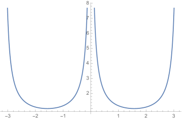
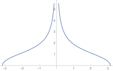
Figure 1. The graphs of the kernels $e^{H_{\alpha}^{(1)}(t)}$ and $e^{H_{\alpha}^{(2)}(t)}$.

The decomposition principle stated in Theorem 2.6 (a) gives rise to the decomposition $Q_{\alpha}=Q^{\prime\prime}_{\alpha/\sqrt{2}}Q^{\prime}_{\alpha/\sqrt{2}}$. We can continue in the same way to decompose $Q^{\prime}_{\alpha/\sqrt{2}}=Q^{\prime\prime}_{\alpha/\sqrt{2}^{2}}Q^{\prime}_{\alpha/\sqrt{2}^{2}}$, so that

$$Q_{\alpha}=Q^{\prime\prime}_{\alpha/\sqrt{2}}Q^{\prime\prime}_{\alpha/\sqrt{2}^{2}}Q^{\prime}_{\alpha/\sqrt{2}^{2}}.$$

The procedure can continue with $Q^{\prime}_{\alpha/\sqrt{2}^{2}}$ and so on

Now let us talk about compositions. Let $Q_{\alpha}$ be the operator by the exponentiation of $\frac{\alpha}{\sqrt{n}}\cos(nt+\omega_{n}^{\prime})$ and let $Q_{\beta}$ be the operator by the exponentiation of $\frac{\beta}{\sqrt{n}}\cos(nt+\omega_{n}^{\prime\prime})$. We suppose that all $\omega_{n}^{\prime}$ and $\omega_{n}^{\prime\prime}$ (for all $n\geq 1$) are independent. By the composition of $Q_{\alpha}$ and $Q_{\beta}$ we mean the operator by the exponentiation of all $\frac{\alpha}{\sqrt{n}}\cos(nt+\omega_{n}^{\prime})$ and $\frac{\beta}{\sqrt{n}}\cos(nt+\omega_{n}^{\prime\prime})$. In other word, it is the operator defined by the weights

$$P_{2n}(t)=\frac{e^{\frac{\alpha}{\sqrt{n}}\cos(nt+\omega_{n}^{\prime})}}{I_{0}(\frac{\alpha}{\sqrt{n}})},\quad P_{2n-1}(t)=\frac{e^{\frac{\beta}{\sqrt{n}}\cos(nt+\omega_{n}^{\prime\prime})}}{I_{0}(\frac{\beta}{\sqrt{n}})}.$$

It is clear that the correlation function of the composition operator is equal to

$$-\frac{\alpha^{2}+\beta^{2}}{2}\log\left|\sin\frac{t}{2}\right|+O(1).$$

This composition operator has the same potential properties as $Q_{\gamma}$ where $\gamma$ verifies

$$\gamma^{2}=\alpha^{2}+\beta^{2}.$$

4.4. Moments with respect to Peyrière measure

Let $\sigma$ be a probability measure on $\mathbb{T}$. If $Q$ acts fully on $\sigma$, we define the Peyrière measure $\mathcal{Q}$ by the following relation

$$\mathbb{E}_{\mathcal{Q}}\phi(t,\omega)=\mathbb{E}\int\phi(t,\omega)dQ\sigma(t).$$

It can be proved that $\{nt+\omega_{n}\mod 2\pi\}$ are $\mathcal{Q}$-independent random variables. This is a little more than what is stated in Theorem 2.5, but the proof is the same. The $\mathcal{Q}$-moment of $\varphi(nt+\omega_{n})$ is easily computed, as stated in the following proposition.

Proposition 4.3.

Let $Q$ be the chaotic operator defined by $\{\alpha_{n}\}$ with $\alpha_{n}\to 0$. Suppose that $\sigma$ is a $Q$-regular probability measure. Let $\mathcal{Q}$ be the Peyrière measure associated to $Q\sigma$. Then for any bounded or non-negative function $\varphi$ we have

(4.4) $$\mathbb{E}_{\mathcal{Q}}\varphi(nt+\omega_{n})=\frac{1}{I_{0}(\alpha_{n})}\int_{0}^{2\pi}\varphi(x)e^{\alpha_{n}\sin x}\frac{dx}{2\pi}.$$

In particular,

$$\mathbb{E}_{\mathcal{Q}}\cos(nt+\omega_{n}) = \frac{I^{\prime}_{0}(\alpha_{n})}{I_{0}(\alpha_{n})}=\frac{1}{2}\alpha_{n}+O(\alpha_{n}^{3})$$

$$\mathbb{E}_{\mathcal{Q}}\cos^{2}(nt+\omega_{n}) = \frac{I^{\prime\prime}_{0}(\alpha_{n})}{I_{0}(\alpha_{n})}=\frac{1}{2}+O(\alpha_{n}^{2})$$

Proof.

The formula (4.4) is a special case of (2.5). From (4.4) and Lemma 3.1, we get immediately the two other estimates. ∎

If we consider $Q_{\alpha}$ defined by $\alpha_{n}=\frac{\alpha}{\sqrt{n}}$, we have

$$\mathbb{E}_{\mathcal{Q}}\cos(nt+\omega_{n}) = \frac{\alpha}{2}\cdot\frac{1}{\sqrt{n}}+O(n^{-3/2})$$

$$\mathbb{E}_{\mathcal{Q}}\cos^{2}(nt+\omega_{n}) = \frac{1}{2}+O(n^{-1})$$

Consequently, we have

Proposition 4.4.

Make the same assumption as in Proposition 4.3. Assume further that $\sum\alpha_{n}^{2}=\infty$. Let $P_{n}(t)$ be the weights defining $Q$. Then for any $\delta>0$, almost surely for $Q\sigma$-almost every $t$ we have

(4.5) $$\sum_{n=1}^{N}\log P_{n}(t)=\frac{1}{4}\sum_{n=1}^{N}\alpha^{2}_{n}+o\left(\left(\sum_{n=1}^{N}\alpha_{n}^{2}\right)^{1/2+\delta}\right).$$

Proof.

Using $\log I_{0}(\alpha_{n})=\frac{1}{4}\alpha_{n}^{2}+O(\alpha_{n}^{4})$ and Proposition 4.3, we get

$$\mathbb{E}_{\mathcal{Q}}\log P_{n}(t)=\alpha_{n}\mathbb{E}_{\mathcal{Q}}\cos(nt+\omega_{n})-\log I_{0}(\alpha_{n})=\frac{1}{4}\alpha^{2}_{n}+O(\alpha_{n}^{4}),$$

and

$$\mathbb{E}_{\mathcal{Q}}(\log P_{n}(t))^{2}$$

$$= \alpha_{n}^{2}\mathbb{E}_{\mathcal{Q}}\cos^{2}(nt+\omega_{n})-2\alpha_{n}\log I_{0}(\alpha_{n})\mathbb{E}_{\mathcal{Q}}\cos(nt+\omega_{n})+\log^{2}I_{0}(\alpha_{n})$$

$$= \frac{1}{4}\alpha^{2}_{n}+O(\alpha_{n}^{4}).$$

So, we get the variance ${\rm Var}_{\mathcal{Q}}(\log P_{n}(t))=\frac{1}{4}\alpha^{2}_{n}+O(\alpha_{n}^{4})$. Let $Y_{n}=\log P_{n}(t)-\mathbb{E}_{\mathcal{Q}}\log P_{n}(t)$. Then the series

$$\sum_{n=1}^{\infty}\frac{Y_{n}}{[{\rm Var}_{\mathcal{Q}}(Y_{1})+\cdots+{\rm Var}_{\mathcal{Q}}(Y_{n})]^{1/2+\delta}}$$

converges $\mathcal{Q}$-a.e. Indeed, since $\{P_{n}\}$ are $\mathcal{Q}$-independent, the partial sums of the series is a $L^{2}$-bounded martingale and Doob’s convergence theorem applies. For the boundedness we use the fact that $\sum\frac{a_{n}}{(a_{1}+\cdots+a_{n})^{c}}<\infty$ for any positive numbers $a_{n}$ and $c>1$. We conclude with the help of Kronecker lemma. ∎

If we consider $Q_{\alpha}$ defined by $\alpha_{n}=\frac{\alpha}{\sqrt{n}}$, we have

(4.6) $$\lim_{N\to\infty}\frac{1}{\log N}\sum_{n=1}^{N}\log P_{n}(t)=\frac{\alpha^{2}}{4}.$$

Intuitively, if $I$ is an interval containing $t$ of length $N^{-1}$, we would have

$$Q_{\alpha}\sigma(I)\asymp P_{1}(t)P_{2}(t)\cdots P_{N}(t)\sigma(I)$$

so that

$$\lim_{|I|\to 0}\frac{\log Q_{\alpha}\sigma(I)}{\log|I|}=-\lim_{N\to\infty}\frac{1}{\log N}\sum_{n=1}^{N}\log P_{n}(t)+\lim_{|I|\to 0}\frac{\log\sigma(I)}{\log|I|}.$$

Therefore $\frac{\alpha^{2}}{4}$ is the difference of dimensions of the measure $\sigma$ and its image $Q_{\alpha}\sigma$:

$$\dim Q_{\alpha}\sigma=\dim\sigma-\frac{\alpha^{2}}{4}.$$

This will be rigorously proved (see Theorem 6.3).

4.5. Mutual singularity and continuity

Let $\{\alpha_{n}\}$ and $\{\alpha_{n}^{\prime}\}$ be two sequences, which defines two operators $Q$ and $Q^{\prime}$ using the same random variables $\{\omega_{n}\}$. There is a simple criterion for the mutual singularity and continuity of $Q\sigma$ and $Q^{\prime}\sigma$.

Proposition 4.5.

Suppose $\sum|\alpha_{n}|^{4}<\infty$ and $\sum|\alpha_{n}^{\prime}|^{4}<\infty$. Suppose that $\sigma$ is a $Q$-regular measure. We have

• $\sum_{n=1}^{\infty}|\alpha_{n}-\alpha_{n}^{\prime}|^{2}<\infty\Rightarrow Q^{\prime}\sigma\ll Q\sigma$ and $\sigma$ is $Q^{\prime}$-regular.

• $\sum_{n=1}^{\infty}|\alpha_{n}-\alpha_{n}^{\prime}|^{2}=\infty\Rightarrow Q^{\prime}\sigma\perp Q\sigma$.

Proof.

This is a special case of Theorem 2.7. Let us compute

$$\mathbb{E}\sqrt{P_{n}(t)P_{n}^{\prime}(t)}=\frac{\mathbb{E}e^{\frac{\alpha_{n}+\alpha_{n}^{\prime}}{2}\cos(nt+\omega)}}{\sqrt{I_{0}(\alpha_{n})I_{0}(\alpha_{n}^{\prime})}}=\frac{I_{0}(\frac{\alpha_{n}+\alpha_{n}^{\prime}}{2})}{\sqrt{I_{0}(\alpha_{n})I_{0}(\alpha_{n}^{\prime})}}.$$

Observe that

$$I_{0}(\frac{\alpha_{n}+\alpha_{n}^{\prime}}{2})=1+\frac{(\alpha_{n}+\alpha_{n}^{\prime})^{2}}{16}+O(\alpha_{n}^{4}+\alpha_{n}^{\prime 4}),$$

$$I_{0}(\alpha_{n})I_{0}(\alpha_{n}^{\prime}) = \left(1+\frac{\alpha^{2}_{n}}{4}+O(\alpha_{n}^{4})\right)\left(1+\frac{{\alpha^{\prime}}^{2}_{n}}{4}+O({\alpha^{\prime}}_{n}^{4})\right)$$

$$= 1+\frac{\alpha_{n}^{2}+{\alpha^{\prime}}_{n}^{2}}{4}+O(\alpha_{n}^{4}+\alpha_{n}^{\prime 4}).$$

It follows that

$$\mathbb{E}\sqrt{P_{n}(t)P_{n}^{\prime}(t)} = \exp\left(\frac{(\alpha_{n}+\alpha_{n}^{\prime})^{2}}{16}-\frac{\alpha_{n}^{2}+{\alpha^{\prime}}_{n}^{2}}{8}+O(\alpha_{n}^{4}+\alpha_{n}^{\prime 4})\right)$$

$$= \exp\left(-\frac{(\alpha_{n}-\alpha_{n}^{\prime})^{2}}{16}+O(\alpha_{n}^{4}+\alpha_{n}^{\prime 4})\right).$$

Finally we conclude by applying Theorem 2.7. ∎

5. Degeneracy

In this section we shall see that the chaotic operator $Q$ can be completely degenerate in the sense that $Q\sigma=0$ for all Borel probability measures $\sigma$. Recall that $H$, defined by (3.3), is the correlation function associated to $Q$. We denote its partial sums by

$$H_{n}(t)=\frac{1}{2}\sum_{k=1}^{n}\alpha_{n}^{2}\cos kt.$$

5.1. A general result

Let

$$S_{n}(t)=\sum_{k=1}^{n}\alpha_{k}\cos(kt+\omega_{k}).$$

The following estimates will allow us to draw conditions for the complete degeneracy in different cases.

Proposition 5.1.

Let $0<h<1$ be a positive number, $n\geq 1$ an integer, $I\subset\mathbb{T}$ an interval and $s\in I$ a fixed point. Let $(p,q)$ a conjugate pair such that $\frac{1}{p}+\frac{1}{q}=1$. We have

(5.1) $$\mathbb{E}\sup_{t\in I}Q_{n}(t)^{h}\leq\left(\mathbb{E}Q_{n}(s)^{hp}\right)^{1/p}\left(\mathbb{E}e^{h|I|q\|S_{n}^{\prime}\|_{\infty}}\right)^{1/q};$$

(5.2) $$\left(\mathbb{E}Q_{n}(s)^{hp}\right)^{1/p}\ll\left[e^{-\frac{1}{4}\cdot\frac{h(1-hp)}{1-h}\sum_{k=1}^{n}\alpha_{k}^{2}}\right]^{1-h};$$

(5.3) $$\left(\mathbb{E}e^{|I|hq\|S_{n}^{\prime}\|_{\infty}}\right)^{1/q}\ll n^{1/q}\exp\left(\frac{h^{2}}{4}q|I|^{2}\sum_{k=1}^{n}k^{2}\alpha_{k}^{2}\right).$$

Proof.

We write

$$Q_{n}(t)=Q_{n}(s)e^{S_{n}(t)-S_{n}(s)}=Q_{n}(s)e^{(t-s)S_{n}^{\prime}(r)}$$

where $r$ is a point between $s$ and $t$, and

$$S_{n}^{\prime}(r)=-\sum_{k=1}^{n}k\alpha_{k}\sin(kr+\omega_{k}).$$

It follows that

$$\sup_{t\in I}Q_{n}(t)^{h}\leq Q_{n}(s)^{h}e^{h|I|\|S_{n}^{\prime}\|_{\infty}}.$$

Thus, by Hölder’s inequality, we get

$$\mathbb{E}\sup_{t\in I}Q_{n}(t)^{h}\leq\left(\mathbb{E}Q_{n}(s)^{hp}\right)^{1/p}\left(\mathbb{E}e^{h|I|q\|S_{n}^{\prime}\|_{\infty}}\right)^{1/q},$$

which is (5.1).

The first expectation on the right hand side in the above inequality is easy to estimate by the independence and the local behavior of the Bessel function $I_{0}(\cdot)$ (cf. Lemma 3.1). Indeed,

$$\mathbb{E}Q_{n}(s)^{hp}=\prod_{k=1}^{n}\frac{I_{0}(hp\alpha_{k})}{I_{0}(\alpha_{k})^{hp}}\ll e^{-\frac{hp-h^{2}p^{2}}{4}\sum_{k=1}^{n}\alpha_{k}^{2}}.$$

Here the assumption $\sum|\alpha_{k}|^{4}<\infty$ is also used. Thus

$$\left(\mathbb{E}Q_{n}(s)^{hp}\right)^{1/p}\ll e^{-\frac{h(1-hp)}{4}\sum_{k=1}^{n}\alpha_{k}^{2}}=\left[e^{-\frac{1}{4}\cdot\frac{h(1-hp)}{1-h}\sum_{k=1}^{n}\alpha_{k}^{2}}\right]^{1-h},$$

which is (5.2).

Now let us prove the last desired estimate. The arguments used below is inspired from [35], p. 68-69). Assume $\|S_{n}^{\prime}\|_{\infty}=|S_{n}^{\prime}(r)|$, where $r$ is a random point. By Bernstein’s inequality, there exists an interval $J$ of length $n^{-1}$ such that $|S^{\prime}(\cdot)|\geq\frac{1}{2}|S^{\prime}(r)|$. Thus

$$e^{|I|hq\|S_{n}^{\prime}\|_{\infty}} \leq \frac{1}{2|J|}\int_{J}e^{|I|hqS_{n}^{\prime}(x)|}dx\leq\frac{n}{2}\int_{\mathbb{T}}e^{|I|hq|S_{n}^{\prime}(x)|}dx.$$

Take the expectation to get

$$\mathbb{E}e^{|I|hq\|S_{n}^{\prime}\|_{\infty}} \leq \frac{n}{2}\int_{\mathbb{T}}\mathbb{E}e^{|I|hq|S_{n}^{\prime}(x)|}dx.$$

$$\leq \frac{n}{2}\int_{\mathbb{T}}\left(\mathbb{E}e^{|I|hqS_{n}^{\prime}(x)}+\mathbb{E}e^{-|I|hqS_{n}^{\prime}(x)}\right)dx.$$

The two last expectations don’t depend on $x$, which can be easily and exactly computed. Thus

$$\mathbb{E}e^{|I|hq\|S_{n}^{\prime}\|_{\infty}}\leq n\prod_{k=1}^{n}I_{0}(|I|hqk\alpha_{k})\ll n\exp\left(\frac{[hq|I|]^{2}}{4}\sum_{k=1}^{n}k^{2}\alpha_{k}^{2}\right).$$

Take $q$-th root of both sides to get (5.3) . ∎

5.2. Degeneracy of $Q_{\alpha}$

Let us apply Proposition 5.1 to treat the special case of $Q_{\alpha}$.

Theorem 5.2.

If $\dim^{*}\sigma<\frac{\alpha^{2}}{4}$, then $Q_{\alpha}\sigma=0$ a.s. In particular, the operator $Q_{\alpha}$ is completely degenerate when $|\alpha|>2$.

Proof.

Since $\alpha_{n}=\frac{\alpha}{\sqrt{n}}$, we have

$$\sum_{k=1}^{n}\alpha_{k}^{2}\sim\alpha^{2}\log n,\qquad\sum_{k=1}^{n}k^{2}\alpha_{k}^{2}\sim\frac{\alpha^{2}}{2}n^{2}.$$

Take a very small $\epsilon>0$. For a given interval $I$, choose $n$ such that $|I|\sim\frac{1}{n^{1+\epsilon}}$. Then choose $q=n^{\epsilon}$, so that $|I|^{2}n^{2}q=O(1)$. Also notice that $n^{1/q}=n^{1/n^{\epsilon}}=O(1)$. So, by Proposition 5.1, we get

$$\mathbb{E}\sup_{t\in I}Q_{n}(t)^{h}\ll\left(\frac{1}{n}\right)^{\frac{\alpha^{2}}{4}\cdot\frac{h(1-hp)}{1-h}(1-h)}\ll|I|^{\frac{\alpha^{2}}{4}\cdot\frac{h(1-hp)}{(1-h)(1+\epsilon)}(1-h)}.$$

Since $\dim^{*}\sigma<\frac{\alpha^{2}}{4}$, for $\epsilon>0$ small enough we have $\dim^{*}\sigma<(1-\epsilon)\frac{\alpha^{2}}{4}$. Take $1>h>1-\epsilon^{2}$. Take $p$ close to $1$ (i.e. $|I|$ is sufficiently small) so that

$$\frac{h(1-hp)}{(1-h)(1+\epsilon)}\geq 1-\epsilon.$$

We have proved that for any small interval $I$ (i.e. $|I|<\delta$ where $\delta$ depends on $\epsilon$ and $p$) there exists an integer $n$ such that

$$\mathbb{E}\sup_{t\in I}Q_{n}(t)^{h}\ll|I|^{\frac{\alpha^{2}}{4}(1-\epsilon)(1-h)}.$$

We conclude for the first assertion by Theorem 2.3. The second assertion is a trivial consequence of the first one. ∎

If $\alpha_{n}=\frac{a_{n}}{\sqrt{n}}$ with $a_{n}\to+\infty$, the operator is completely degenerate.

6. Image and kernel of the projection $\mathbb{E}Q_{\alpha}$

Now we are going to show that if $\sigma$ is rather regular in the sense of Riesz potential theory, then it is $Q_{\alpha}$-regular. The following theorem gives an exact statement. This result and Theorem 5.2 on the degeneracy will give us a satisfactory description of the image and kernel of the projection $\mathbb{E}Q_{\alpha}$. It is then possible to compute the dimension of $Q_{\alpha}\sigma$.

6.1. $Q_{\alpha}$-regular measures

Theorem 6.1.

Suppose that $D>\frac{\alpha^{2}}{4}$. If $\sigma\in\mathcal{R}_{D}^{*}$, then $Q_{\alpha}\sigma\in\mathcal{R}_{D-\frac{\alpha^{2}}{4}}^{*}$.

Proof.

We shall follow [36]. The method was also used in [24]. By the hypothesis on $\sigma$, for any $\epsilon>0$ there exist a number $\eta>D$ and a compact set $K$ such that $\sigma(K^{c})<\epsilon$ and

$$I_{\eta}(\sigma 1_{K})=\int_{K}\int_{K}\frac{d\sigma(t)d\sigma(s)}{|t-s|^{\eta}}<\infty.$$

Step I. We first suppose that $D>\frac{\alpha^{2}}{2}$. By the $L^{2}$-theory (Proposition 4.1), $\mathbb{E}Q_{\alpha}\sigma_{K}=\sigma_{K}$, where $\sigma_{K}$ is the restriction $\sigma 1_{K}$. The associated Peyrière measure $\mathcal{Q}_{K}$ is well defined. Denote by $R_{n}$ the chaotic operator defined by the weights $P_{m}$ with $m\geq e^{n}$ and consider the mass of $R_{n}\sigma_{K}$ concentrated in the ball $B(t,e^{-n})$ centered at $t$ of radius $e^{-n}$:

$$\rho_{n}(t)=R_{n}\sigma_{K}(B(t,e^{-n})),$$

which can be rewritten as

$$\rho_{n}(t)=\int\chi_{n}(t,s)dR_{n}\sigma(s)$$

where $\chi_{n}(t,s)$ is the characteristic function of the set of the points $(t,s)\in K\times K$ such that $|t-s|\leq e^{-n}$. We can then compute the $\mathcal{Q}_{K}$-expectation of $\rho_{n}$. Indeed, by the definition of $\mathcal{Q}_{K}$ and Proposition 4.1, we have

$$\mathbb{E}_{\mathcal{Q}_{K}}\rho_{n}=\int\int\chi_{n}(t,s)\prod_{m=[e^{n}]}^{\infty}\mathbb{E}P_{m}(t)P_{m}(s)d\sigma_{K}(t)d\sigma_{K}(s).$$

Notice that

$$\sum_{m=1}^{[e^{n}]}\mathbb{E}P_{m}(t)P_{m}(s)=\exp\left(\frac{\alpha^{2}}{2}\sum_{m=1}^{[e^{n}]}\frac{\cos m(t-s)}{m}+O(1)\right).$$

If $|t-s|\leq e^{-n}$, then

$$\sum_{m=1}^{[e^{n}]}\mathbb{E}P_{m}(t)P_{m}(s)=\exp\left(\frac{\alpha^{2}}{2}n+O(1)\right).$$

Therefore

$$\mathbb{E}_{\mathcal{Q}_{K}}\rho_{n}\ll\int\int e^{-\frac{\alpha^{2}}{2}n}\frac{\chi_{n}(t,s)}{\left|\sin\frac{t-s}{2}\right|^{\frac{\alpha^{2}}{2}}}d\sigma_{K}(t)d\sigma_{K}(s).$$

If $\chi_{n}(t,s)=1$, we have $e^{n}\leq 1/|t-s|$ so that

$$\sum_{m=1}^{\infty}e^{(\eta-\frac{\alpha^{2}}{2})n}\frac{\chi_{n}(t,s)}{\left|\sin\frac{t-s}{2}\right|^{\frac{\alpha^{2}}{2}}}\ll\frac{1}{|t-s|^{\eta}},$$

It follows that

$$\mathbb{E}_{\mathcal{Q}_{K}}\left(\sum_{m=1}^{\infty}e^{\eta n}\rho_{n}\right)<\infty$$

and consequently $\rho_{n}=O(e^{-\eta n})$ $\mathcal{Q}_{K}$-a.s. So, almost surely

$$\rho_{n}(t)=O(e^{-\eta n})\,\,\,\,\quad Q_{\alpha}\sigma_{K}\!-\!a.e.$$

Then for any $\epsilon>0$, almost surely there exists a compact subset $K_{\epsilon}^{1}\subset K$ such that

$$Q_{\alpha}\sigma(K\setminus K_{\epsilon}^{1})<\epsilon$$

$$\limsup_{n\rightarrow\infty}\frac{\log\rho_{n}(t)}{n}\leq-\eta\,\,\,{\rm uniformly\ on}\,K_{\epsilon}^{1}.$$

On the other hand, from Proposition 4.4 we can deduce that almost surely for every $\epsilon>0$, there exists a compact set $K_{\epsilon}^{2}$ contained in $K$ such that

$$Q_{\alpha}\sigma(K\setminus K_{\epsilon}^{2})<\epsilon$$

$$\frac{\log Q_{n}(t)}{\log n}\rightarrow\frac{\alpha^{2}}{4}\,\,\,{\rm uniformly\,on}\,K_{\epsilon}^{2}.$$

Now let

$$S_{\epsilon}=1_{K_{\epsilon}^{1}\bigcap K_{\epsilon}^{2}}Q\sigma.$$

Then

$$Q\sigma(K\setminus(K_{\epsilon}^{1}\bigcap K_{\epsilon}^{2}))<2\epsilon,$$

and

$$\limsup_{n\rightarrow\infty}\frac{\log S_{\epsilon}(B(t,e^{-n}))}{n}\leq\limsup_{n\rightarrow\infty}\frac{\log Q_{[e^{dn}]}(t)}{n}+\limsup_{n\rightarrow\infty}\frac{\log\rho_{n}(t)}{n}\leq\frac{\alpha^{2}}{4}-\eta$$

uniformly on $K_{\epsilon}^{1}\bigcap K_{\epsilon}^{2}$. This implies $Q_{\alpha}\sigma\in M_{(D-\frac{\alpha^{2}}{4})^{+}}^{+}({\mathbb{T}})$. Let us summarize as follows

(6.1) $$D>\frac{\alpha^{2}}{2},\ \ \sigma\in\mathcal{R}^{*}_{D}\Longrightarrow Q_{\alpha}\sigma_{K}\in\mathcal{R}^{*}_{D-\frac{\alpha^{2}}{4}},$$

where $\sigma(K^{c})$ can be made as small as we like.

Step II. General case. We use the decomposition

$$Q_{\alpha}=Q^{(m)}_{\frac{\alpha}{\sqrt{2}^{m}}}Q^{\prime}_{\frac{\alpha}{\sqrt{2}^{m}}}\cdots Q^{\prime}_{\frac{\alpha}{\sqrt{2}^{2}}}Q^{\prime}_{\frac{\alpha}{\sqrt{2}}}$$

which is presented in §4.3. First apply the principle (6.1) to $Q^{\prime}_{\frac{\alpha}{\sqrt{2}}}$ and $\sigma$. We check that $D>\frac{\alpha^{2}}{4}=\frac{(\alpha/\sqrt{2})^{2}}{2}$ and $\sigma\in\mathcal{R}^{*}_{D}$, and we get

$$Q^{\prime}_{\frac{\alpha}{\sqrt{2}}}\sigma\in\mathcal{R}^{*}_{D-\frac{\alpha^{2}}{4\cdot 2}}.$$

Now observe that $D-\frac{\alpha^{2}}{4\cdot 2}>\frac{\alpha^{2}}{8}=\frac{(\frac{\alpha}{\sqrt{2}^{2}})^{2}}{2}$. So, the principle (6.1) applies $Q^{\prime}_{\frac{\alpha}{\sqrt{2}^{2}}}$ and $Q^{\prime}_{\frac{\alpha}{\sqrt{2}}}\sigma$. Thus we get

$$Q^{\prime}_{\frac{\alpha}{\sqrt{2}^{2}}}Q^{\prime}_{\frac{\alpha}{\sqrt{2}}}\sigma\in\mathcal{R}^{*}_{D-\frac{\alpha^{2}}{4\cdot 2}-\frac{\alpha^{2}}{4\cdot 2^{2}}}.$$

Inductively we get

$$Q^{\prime}_{\frac{\alpha}{\sqrt{2}^{m}}}\cdots Q^{\prime}_{\frac{\alpha}{\sqrt{2}^{2}}}Q^{\prime}_{\frac{\alpha}{\sqrt{2}}}\sigma\in\mathcal{R}^{*}_{D-\frac{\alpha^{2}}{4\cdot 2}-\frac{\alpha^{2}}{4\cdot 2^{2}}-\cdots-\frac{\alpha^{2}}{4\cdot 2^{m}}}.$$

Since $D-\frac{\alpha^{2}}{4}>0$. When $m$ is sufficiently large, we have

$$D-\frac{\alpha^{2}}{4\cdot 2}-\frac{\alpha^{2}}{4\cdot 2^{2}}-\cdots-\frac{\alpha^{2}}{4\cdot 2^{m}}>\frac{(\alpha/\sqrt{2}^{m})^{2}}{2}=\frac{\alpha^{2}}{2^{m+1}}.$$

So, we can apply once more the principle (6.1), to $Q^{(m)}_{\frac{\alpha}{\sqrt{2}^{m}}}$. Finally we get

$$Q^{(m)}_{\frac{\alpha}{\sqrt{2}^{m}}}Q^{\prime}_{\frac{\alpha}{\sqrt{2}^{m}}}\cdots Q^{\prime}_{\frac{\alpha}{\sqrt{2}^{2}}}Q^{\prime}_{\frac{\alpha}{\sqrt{2}}}\sigma\in\mathcal{R}^{*}_{D-\frac{\alpha^{2}}{4\cdot 2}-\frac{\alpha^{2}}{4\cdot 2^{2}}-\cdots-\frac{\alpha^{2}}{4\cdot 2^{m}}-\frac{\alpha^{2}}{4\cdot 2^{m}}}=\mathcal{R}^{*}_{D-\frac{\alpha^{2}}{4\cdot 2}}.$$

∎

6.2. ${\rm Ker}\,\mathbb{E}Q_{\alpha}$ and ${\rm Im}\,\mathbb{E}Q_{\alpha}$

We have the following description for the kernel and the image $\mathbb{E}Q_{\alpha}$.

Theorem 6.2.

We have

$$\mathcal{S}_{\frac{\alpha^{2}}{4}-}\subset{\rm Ker}\mathbb{E}Q_{\alpha}\subset\mathcal{S}_{\frac{\alpha^{2}}{4}+};$$

$$\mathcal{R}_{\frac{\alpha^{2}}{4}+}\subset{\rm Im}\ \mathbb{E}Q_{\alpha}\subset\mathcal{R}_{\frac{\alpha^{2}}{4}-}.$$

Proof.

The first inclusion follows immediately from Theorem 5.2. Now we prove the second inclusion by contradiction. Suppose $\sigma\in{\rm Ker}\mathbb{E}Q_{\alpha}$ but $\sigma\not\in\mathcal{S}_{\frac{\alpha^{2}}{4}+}$. Then $\sigma\in\mathcal{S}^{c}_{\beta}$ for some $\beta>\frac{\alpha^{2}}{4}$. That means $\sigma$ has its $\beta$-regular component $\sigma_{r}\not=0$ according to the Kahane decomposition. Hence, by Theorem 6.1,

$$\dim_{*}Q_{\alpha}\sigma\geq\dim_{*}Q_{\alpha}\sigma_{r}\geq\beta-\frac{\alpha^{2}}{4}>0\quad a.s$$

which contradicts $\sigma\in{\rm Ker}\mathbb{E}Q_{\alpha}$.

Assume $\sigma\in\mathcal{R}_{\frac{\alpha^{2}}{4}+}$. That means $\sigma\in\mathcal{R}_{\beta}$ for some $\beta>{\frac{\alpha^{2}}{4}}$. We claim that $\sigma\in{\rm Im}\ \mathbb{E}Q_{\alpha}$. Otherwise, there is a non null component of $\sigma$, say $\sigma 1_{K}$ with $\sigma(K)>0$, which is killed by $\mathbb{E}Q_{\alpha}$. That is to say, $\sigma 1_{K}\in{\rm Ker}\mathbb{E}Q_{\alpha}$. So, $\sigma 1_{K}\in\mathcal{S}_{\frac{\alpha^{2}}{4}+}$, by what we have just proved above. Hence ${\rm Cap}_{\beta}(K)=0$. This contradicts $\sigma 1_{K}\in\mathcal{R}_{\beta}$.

The last inclusion is also proved by contradiction. Assume $\sigma\in\mathbb{E}Q_{\alpha}$ but $\sigma\not\in\mathcal{R}_{\frac{\alpha^{2}}{4}-}$. Then $\sigma\not\in\mathcal{R}_{\beta}$ for some $\beta<\frac{\alpha^{2}}{4}$. By the Kahane decomposition, $\sigma$ has a non null $\beta$-singular component which must be killed by $\mathbb{E}Q_{\alpha}$ because $\beta<\frac{\alpha^{2}}{4}$ (cf. Theorem 5.2). This contradicts $\sigma\in\mathbb{E}Q_{\alpha}$. ∎

Recall that $\dim\sigma=D$ means $\dim_{*}\sigma=\dim^{*}\sigma=D$. In this case, we say that $\sigma$ is unidimensional. The dimension of $Q_{\alpha}\sigma$ is given by the following formula.

Theorem 6.3.

Suppose that $\sigma$ is a unidimensional measure and $\dim\sigma>\frac{\alpha^{2}}{4}$. We have

$$\dim Q_{\alpha}\sigma=\dim\sigma-\frac{\alpha^{2}}{4}.$$

Proof.

Let $D=\dim\sigma$. For any $\epsilon>0$, the fact $\dim_{*}\sigma=D$ implies $\sigma\in\mathcal{R}^{*}_{D-\epsilon}$. Then by Theorem 6.1, we get $\dim_{*}Q_{\alpha}\sigma\geq D-\epsilon-\frac{\alpha^{2}}{4}$ a.s. This proves $\dim_{*}Q_{\alpha}\sigma\geq D-\frac{\alpha^{2}}{4}$ a.s.

Take $\beta$ such that $\frac{\beta^{2}}{4}+\frac{\alpha^{2}}{4}>D$. Let $\gamma$ be such that $\gamma^{2}=\beta^{2}+\alpha^{2}$. We consider an operator $Q_{\beta}$, which is independent of $Q_{\alpha}$. The product $Q_{\beta}Q_{\alpha}$ has the same law as $Q_{\gamma}$. The fact $\dim^{*}\sigma=D$, together with $\frac{\beta^{2}}{4}+\frac{\beta^{2}}{4}>D$, implies $\sigma\in{\rm Ker}\mathbb{E}Q_{\gamma}$. Then, by Theorem 2.6 c), we get $Q_{\alpha}\sigma\in{\rm Ker}\mathbb{E}Q_{\beta}$ a.s. Now we apply Theorem 6.2 to get $\dim^{*}Q_{\alpha}\sigma\leq\beta$ a.s. Optimizing $\beta$ leads to $\dim^{*}Q_{\alpha}\sigma\leq D-\frac{\alpha^{2}}{4}$ a.s. ∎

7. Trigonometric multiplicative chaos on $\mathbb{T}^{d}$

Our theory can be extended to torus $\mathbb{T}^{d}$ of all dimensions, with few points to be checked in higher dimension case. On $\mathbb{T}^{d}$ we propose to study the random series

(7.1) $$\sum_{n\in\mathbb{Z}^{d}_{+}}\rho_{n}\cos(n\cdot x+\omega_{n})$$

where $\mathbb{Z}^{d}_{+}$ is the set $\mathbb{Z}^{d}\setminus\{0\}$ but with $n$ and $-n$ identified, and $\{\omega_{n}\}$ are iid random variables uniformly distributed on $\mathbb{T}$ (not on $\mathbb{T}^{d}$). It can be rewritten as

$$\frac{1}{2}\sum_{n\in\mathbb{Z}^{d}\setminus\{0\}}\rho_{n}e^{i(n\cdot x+\omega_{n})}$$

with $\rho_{n}=\rho_{-n}$ and $\omega_{n}=\omega_{-n}$. When, $d=1$, $\mathbb{Z}^{d}_{+}$ is the set of natural numbers. The correlation function of (7.1) is defined by

$$H(t)=\frac{1}{2}\ \sum_{n\in\mathbb{Z}^{d}_{+}}\rho_{n}^{2}\cos(n\cdot t)\qquad(t\in\mathbb{T}^{d}).$$

Let $|x|_{\infty}=\max_{1\leq i\leq d}|x_{j}|$ for $x=(x_{1},\cdots,x_{d})\in\mathbb{R}^{d}$. Let $|x|$ to denote the euclidean norm $\sqrt{\sum_{i=1}^{n}x_{i}^{2}}$.

7.1. Definition of $\mathbb{T}^{d}$-martingales

Let $\{\alpha_{k}\}_{k\in\mathbb{Z}^{d}_{+}}$ be a family of real numbers such that $\sum_{k\in\mathbb{Z}^{d}_{+}}|\alpha_{k}|^{4}<\infty$. Let $\{A_{n}\}$ be an increasing sequence of finite subsets of $\mathbb{Z}^{d}_{+}$ such that $A_{n}\uparrow\mathbb{Z}^{d}_{+}$ with $A_{0}=\emptyset$. We define the weights

(7.2) $$P_{n}(t)=\frac{\exp\sum_{k\in A_{n}\setminus A_{n-1}}\alpha_{k}\cos(k\cdot t+\omega_{k})}{\prod_{k\in A_{n}\setminus A_{n-1}}I_{0}(\alpha_{k})}.$$

Here is a choice for $\{A_{n}\}$. For $n\geq 1$, we consider the hypercube $C_{n}=\{k\in\mathbb{Z}^{d}:|k|_{\infty}\leq n\}$ and choose $A_{n}$ to the positive part $C_{n}^{+}=C_{n}\cap\mathbb{Z}^{d}_{+}$. In this case $C_{n}^{+}\setminus C_{n-1}^{+}$ is the boundary $\partial C_{n}^{+}$. We have $\#C_{n}=(2n+1)^{d}-1$. It follows that

$$\#C_{n}^{+}=\frac{(2n+1)^{d}-1}{2},\qquad\#\partial C_{n}^{+}\sim d2^{d-1}n^{d-1}.$$

Another choice for $A_{n}$ is the ball $\{k\in\mathbb{Z}^{d}_{+}:|k|\leq n\}$.

The $\mathbb{T}^{d}$-martingale defined by the weight (7.2) produces a chaotic operator $Q$. The same computation as in the case of dimension $1$ leads to the basic relation

(7.3) $$\mathbb{E}Q_{n}(t)Q_{n}(s)=\exp\left(\frac{1}{2}\sum_{k\in A_{n}}\alpha_{k}^{2}\cos k\cdot(t-s)+O(1)\right).$$

For a given real number $\alpha$, we have the typical sequence of coefficients

$$\alpha_{k}=\frac{\alpha}{|k|^{d/2}}.$$

As we shall see below (cf. Theorem 7.1), the corresponding correlation function $H_{\alpha}(t)$ is smooth in $\mathbb{T}^{d}\setminus\{0\}$ and around $0$ it behaves as

$$H_{\alpha}(t)=\frac{\alpha^{2}}{2}\sum_{k\in\mathbb{Z}^{d}_{+}}\frac{\cos k\cdot t}{|k|^{d}}\sim\frac{\alpha^{2}}{2}\cdot\frac{\pi^{d/2}}{\Gamma(d/2)}\log\frac{1}{|t|}\quad(t\to 0).$$

Its exponentiation $\Phi_{\alpha}=e^{H_{\alpha}(t)}$ is then a Riesz kernel

(7.4) $$\Phi_{\alpha}(t)\asymp\frac{1}{|t|^{\tau(\alpha)\alpha^{2}/2}}\qquad{\rm with}\ \ \ \tau(\alpha)=\frac{\pi^{d/2}}{\Gamma(d/2)}.$$

7.2. Correlation function $H_{\alpha}$

We consider the Jacobi function $G$ defined by the trigonometric series

(7.5) $$G(x)=\sum_{k\in{\mathbb{Z}}^{d},k\neq 0}|k|^{-d}\exp(ik\cdot x).$$

For $m\geq 1$, we denote by $S_{m}$ its partial sum:

$$S_{m}(G)=\sum_{|k|\leq m,k\neq 0}|k|^{-d}\exp(ik\cdot x).$$

We set $s_{d}=2\frac{\pi^{d/2}}{\Gamma(d/2)}$ which is the area of the unit sphere in $\mathbb{R}^{d}$.

Theorem 7.1.

The Jacobi function $G$ has the following properties:
(a) The function $G(x)$ is ${\mathcal{C}}^{\infty}$ in ${\mathbb{T}}^{d}\setminus\{0\}.$
(b)  There is a bounded function $E(x)$ on $\mathbb{T}^{d}$ such that

$$\forall x\in\mathbb{T}^{d},\ \ \ \ G(x)=s_{d}\log\frac{1}{|x|}+E(x).$$

(c) There exists a constant $C$ such that for any integer $m\geq 1$ we have

$$S_{m}(G)(x)\leq s_{d}\log\frac{1}{|x|}+C.$$

Proof.

The proof mimics the argument given by Titchmarsh and Riemann himself of the functional equation of the zeta function. One considers the Jacobi function $\theta(u,x)$ defined by

$$\theta(u,x)=\sum_{n\in\mathbb{Z}^{d}}\exp(-|n|^{2}u)\exp(in\cdot x).$$

Here $u>0$ and $x\in\mathbb{T}^{d}$. The notations used here slightly differ from the standard ones. Let us consider $\theta_{0}=\theta-1$. Then the function $\theta_{0}(u,x)$ has an exponential decay as $u$ tends to $+\infty$ and this decay is uniform in $x$. Assume $s>d$. We introduce the auxiliary Jacobi functions

$$G(s,x)=\sum_{n\in\mathbb{Z}^{d},n\neq 0}|n|^{-s}\exp(in\cdot x).$$

where the series converges absolutely. Fubini theorem implies

$$\int_{0}^{\infty}\theta_{0}(u,x)u^{s/2}\frac{du}{u}=\Gamma(s/2)G(s,x).$$

One splits this integral into $\int_{0}^{1}+\int_{1}^{\infty}$ which yields

$$\Gamma(s/2)G(s,x)=A(s,x)+B(s,x).$$

The function $B(s,\cdot)$ is obviously a $C^{\infty}$ function for every $s\geq 0$, especially $B(d,x)$. To study $A(s,x)$, one rewrites $\theta_{0}=\theta-1$ and uses the following functional equation for the Jacobi function

$$\theta(u,x)=\frac{\pi^{d/2}}{u^{d/2}}\sum_{k\in\mathbb{Z}^{d}}\exp\Big{(}-\frac{|x-2\pi k|^{2}}{4u}\Big{)},$$

which follows from the Poisson summation formula. One can ignore $1$ in $\theta_{0}=\theta-1$ since its contribution to $A(s,x)$ yields a constant. When $x$ belongs to the ball centered at $0$ with radius $1$ all the terms together in the above sum but the term $k=0$ yield a ${\mathcal{C}}^{\infty}$ contribution. Therefore one is led to

$$J(s,x):=\pi^{d/2}\int_{0}^{1}\exp\left(-\frac{|x|^{2}}{4u}\right)u^{\frac{s-d}{2}}\frac{du}{u}.$$

We have thus proved the following lemma.

Lemma 7.2.

The difference

(7.6) $$\Gamma(s/2)G(s,x)-J(s,x)=R(s,x)$$

is a ${\mathcal{C}}^{\infty}$ function for every $s\geq 0$.

Therefore one can pass to the limit $s\to d$ in (7.6) and we are led to the computation of $J(d,x)$. Make a change of variables $t=\frac{|x|^{2}}{4}u$ we get

$$J(d,x)=\pi^{d/2}\int_{0}^{\frac{4}{x^{2}}}e^{-\frac{1}{t}}\frac{dt}{t}=2\pi^{d/2}\log\frac{1}{|x|}+O(1),\qquad x\to 0.$$

We have thus proved (a) and (b).

(c) will follow from (a), (b) and the following lemma.

Lemma 7.3.

If $\phi$ denotes a non negative compactly supported radial function of integral $1$ and if $\phi_{m}(x)=m^{d}\phi(mx)$ we have

$$\|G*\phi_{m}-S_{m}(G)\|_{\infty}\leq C.$$

The proof of this lemma is immediate. We have

$$|{\widehat{\phi}}\big{(}\frac{y}{m}\big{)}-1|\leq C\frac{|y|^{2}}{m^{2}}\ \ {\rm if}\ \ |y|\leq m;\quad|{\widehat{\phi}}\big{(}\frac{y}{m}\big{)}|\leq C\frac{m^{2}}{|y|^{2}}\ \ {\rm if}\ \ |y|\geq m.$$

This together with the decay of the Fourier coefficients of $G$ yields the result.

Now prove (c). By (a) and (b), the function $G$ can be forgotten and replaced by $f(x)=s_{d}|\log|x||$, because the question arises around $0$. It suffices to check that $f*\phi_{m}\leq f+C$ which is an easy calculation. ∎

It is easy to deduce that the partial sums over cubes $C_{n}$ are also bounded by $s_{d}\log(1/|x|)+C$.

7.3. Riesz potential theory on $\mathbb{T}^{d}$ and $L^{2}$-theory

Let $\beta\in(0,d)$ be a fixed number. It is known that (cf. [55], p. 256)

$$\sum_{m\in\mathbb{Z}^{d},m\not=0}\frac{1}{|m|^{d-\beta}}e^{im\cdot x}\sim\gamma_{\beta}\frac{1}{|x|^{\beta}}+b(x)$$

where $\gamma_{\beta}=2^{\beta}\pi^{2\beta-\frac{d}{2}}\frac{\Gamma(\frac{d-\beta}{2})}{\Gamma(\frac{\beta}{2})}$ and $b\in C^{\infty}(\mathbb{T}^{d})$. This means that the function on the right, which is Lebesgue integrable on $\mathbb{T}^{d}$, admits the series on the left as its Fourier series. The function $b$ is necessarily real valued. Let $B=\max_{x}b(x)$. We define the $\beta$-order Riesz kernel by

$$R_{\beta}(x)=\gamma_{\beta}\frac{1}{|x|^{\beta}}+b(x)+B.$$

It is a positive, lower semicontinuous function having positive Fourier coefficients. We also have the following simple estimate

$$R_{\beta}(x)\asymp\frac{1}{|x|^{\beta}}\qquad(|x_{1}|\leq\pi,\cdots,|x_{d}|\leq\pi).$$

As in the case $d=1$, the $\beta$-order energy $I^{\sigma}_{\beta}$ of a measure $\sigma$ on $\mathbb{T}^{d}$ can be defined. As shown in [42], we have the formula

$$I^{\sigma}_{\beta}=B|\widehat{\sigma}(0)|^{2}+\sum_{|m|>0}\frac{|\widehat{\sigma}(m)|^{2}}{|m|^{d-\beta}}.$$

More generally we have the results on $\mathbb{T}^{d}$ as developed in §3.3 about potential, capacity and dimension (cf. [42],[39], [21]).

By Theorem 7.1, we have

$$H_{\alpha}(t)=\frac{\alpha}{2}\cdot\frac{\pi^{d/2}}{\Gamma(d/2)}\log\frac{1}{|t|}+O(1)\quad({\rm as}\ \ t\to 0).$$

Theorem 7.1 allows us to develop the $L^{2}$-theory for our $\mathbb{T}^{d}$-martingales, which was developed in §4 for the case $d=1$. We don’t restate the results here, but we are free to use them.

7.4. Degeneracy

Proposition 7.4.

The result of Proposition 5.1 remain true when $d\geq 2$. It suffices to replace $\sum_{k=1}^{n}\alpha_{k}^{2}$ and $\sum_{k=1}^{n}k^{2}\alpha_{k}^{2}$ respectively by

$$\sum_{k\in A_{n}}\alpha_{k}^{2},\qquad\sum_{k\in A_{n}}|k|^{2}\alpha_{k}^{2}.$$

Proof.

The proof is the same as that of Proposition 5.1. We only need to point out one point. Let

$$S_{n}(t)=\sum_{k\in A_{n}}\alpha_{k}\cos(k\cdot t+\omega).$$

Now

$$|S_{n}(t)-S_{n}(s)|=\left|\sum_{j=1}^{d}\frac{\partial S_{n}}{\partial t_{j}}(r)(t_{j}-s_{j})\right|\leq|t-s|_{\infty}\sum_{j=1}^{d}\left|\frac{\partial S_{n}}{\partial t_{j}}(r)\right|,$$

where

$$\frac{\partial S_{n}}{\partial t_{j}}(r)=-\sum_{k\in A_{n}}k_{j}\alpha_{k}\sin(k\cdot t+\omega)$$

Let $I$ be a cube and let $|I|$ be its side length. We would have to estimate the following expectation

$$\mathbb{E}\exp\left(h|I|q\sum_{j=1}^{d}\left\|\frac{\partial S_{n}}{\partial t_{j}}\right\|_{\infty}\right),$$

which, by Hölder inequality, is bounded by

$$\left\{\prod_{j=1}^{d}\mathbb{E}\exp\left(dh|I|q\left\|\frac{\partial S_{n}}{\partial t_{j}}\right\|_{\infty}\right)\right\}^{1/d}$$

Each of these expectation can be estimated as before. Finally we get

$$\mathbb{E}\exp\left(h|I|q\sum_{j=1}^{d}\left\|\frac{\partial S_{n}}{\partial t_{j}}\right\|_{\infty}\right)\ll n\exp\left(\frac{d[hq|I|]^{2}}{4}(k_{1}^{2}+\cdots+k_{d}^{2})\alpha_{k}^{2}\right).$$

∎

Let us apply the result to the special case $\alpha_{k}=\frac{\alpha}{|k|^{d/2}}$. Let us take $A_{n}=C_{n}^{+}$. We are led to estimate

$$\sum_{k\in C_{n}^{+}}\alpha_{k}^{2}=\sum_{k\in C_{n}^{+}}\frac{\alpha^{2}}{|k|^{d}},\qquad\sum_{k\in C_{n}^{+}}|k|^{2}\alpha_{k}^{2}=\sum_{k\in C_{n}^{+}}\frac{\alpha^{2}}{|k|^{d-2}}.$$

The sum over $C_{n}$ doubles the sum over $C_{n}^{+}$. The sum over $C_{n}$ and the sum over the ball $B(0,n)$ are comparable, because the cube $C_{n}$ is contained in the ball centered at $0$ of radius $\sqrt{d}n$, and contains the ball of radius $n$.

Lemma 7.5.

Let $B(0,R)$ be the ball of radius $R$ centered at $0$. We have

$$\sum_{1\leq|k|\leq R}\frac{1}{|k|^{d}}=s_{d}\log R+O(1),\qquad\sum_{1\leq|k|\leq R}\frac{1}{|k|^{d-2}}=s_{d}R^{2}+O(R).$$

where $s_{d}=2\frac{\pi^{d/2}}{\Gamma(d/2)}$. Also we have

$$\int_{n\leq|x|\leq\sqrt{d}n}\frac{dx}{|x|^{d}}=O(1),\qquad\int_{n\leq|x|\leq\sqrt{d}n}\frac{dx}{|x|^{d-2}}\asymp n^{2}.$$

Proof.

Assume $d\geq 2$. When $x$ is in the unit cube centered by $k$, we have $|k|^{-d}-|x|^{-d}=O(|k|^{-(d+1)})$. Since $\sum|k|^{-(d+1)}<\infty$, we have

$$\sum_{1\leq|k|\leq R}\frac{1}{|k|^{d}}=\int_{1\leq|x|\leq R}\frac{dx}{|x|^{d}}+O(1).$$

The integral is equal to $s_{d}\int_{1}^{R}\frac{dr}{r}=s_{d}\log R$. The second equality can be proved in the same. We need the estimate $|k|^{-d+2}-|x|^{-d+2}=O(|k|^{-(d-1)})$ for $x$ in the unit cube centered by $k$. The estimates of two integrals are direct. ∎

This lemma implies

$$\sum_{k\in C_{n}^{+}}\alpha_{k}^{2} = \sum_{k\in C_{n}^{+}}\frac{\alpha^{2}}{|k|^{d}}=\frac{\alpha^{2}}{2}s_{d}\log n+O(1),$$

$$\qquad\sum_{k\in C_{n}^{+}}|k|^{2}\alpha_{k}^{2} = \sum_{k\in C_{n}^{+}}\frac{\alpha^{2}}{|k|^{d-2}}=\frac{\alpha^{2}}{2}s_{d}n^{2}+O(n).$$

Now we are ready to state the following theorem which we can prove using the last two estimate and the same proof of Theorem 5.2.

Theorem 7.6.

Let us consider the operator $Q_{\alpha}$ on $\mathbb{T}^{d}$ with $d\geq 2$. If $\dim\sigma^{*}<\frac{\alpha^{2}}{4}\frac{s_{d}}{2}=\frac{\alpha^{2}}{4}\frac{\pi^{d/2}}{\Gamma(d/2)}$, then $Q_{\alpha}\sigma=0$. Consequently, the operator $Q_{\alpha}$ is completely degenerate when $|\alpha|^{2}>4d\frac{\Gamma(d/2)}{\pi^{d/2}}$.

The about statement coincides with $d=1$ if we define $s_{1}=2$. So, the degeneracy condition $|\alpha|^{2}>4d\frac{\Gamma(d/2)}{\pi^{d/2}}$ holds for all $d\geq 1$.

7.5. Decomposition of $H_{\alpha}$ and $Q_{\alpha}$, kernel and image of $\mathbb{E}Q_{\alpha}$

The following result was known for $d=1$ (cf. §4.3). It will allows us to decompose the operator $Q_{\alpha}$ in a suitable way. Recall that the function $G$ is defined by (7.5).

Lemma 7.7.

There is a partition of $\mathbb{Z}^{d}\setminus\{0\}$ into two parts $\mathcal{P}_{1}$ and $\mathcal{P}_{2}$ such that the decomposition $G=G_{1}+G_{2}$ with

$$G_{1}(x)=\sum_{k\in\mathcal{P}_{1}}|k|^{-d}\exp(ik\cdot x),\qquad G_{2}(x)=\sum_{k\in\mathcal{P}_{2}}|k|^{-d}\exp(ik\cdot x)$$

has the property

$$G_{1}(x)=\frac{1}{2}G(x)+O(1),\quad G_{1}(x)=\frac{1}{2}G(x)+O(1)\ \ \ {\rm as}\ x\to 0.$$

The partial sums, cubic or spheric, of both $G_{1}$ and $G_{2}$ are respectively bounded by $G_{1}(x)+C$ or $G_{2}(x)+C$ for some constant $C$.

Proof.

We first look at the case $d=2$. Let

$$A=\begin{pmatrix}1&-1\\ 1&1\end{pmatrix}=\sqrt{2}\begin{pmatrix}\cos\frac{\pi}{4}&-\sin\frac{\pi}{4}\\ \sin\frac{\pi}{4}&\ \cos\frac{\pi}{4}\end{pmatrix}.$$

The linear map defined by $A$ is a similitude such that $|Ak|=2|k|$ and preserves the lattice $\mathbb{Z}^{d}$. We choose $\mathcal{P}_{1}=A(\mathbb{Z}^{d}\setminus\{0\})$ and $\mathcal{P}_{2}=\mathbb{Z}^{d}\setminus\{0\}\setminus\mathcal{P}_{1}$. Then

$$G_{1}(x)=\sum_{k\in\mathbb{Z}^{d}\setminus\{0\}}|Ak|^{-d}\exp(iAk\cdot x)=\frac{1}{2}\sum_{k\in\mathbb{Z}^{d}\setminus\{0\}}|k|^{-d}\exp(ik\cdot\,^{t}\!Ax).$$

Now, by Theorem 7.1, around $0$ we have

$$G_{1}(x)=\frac{1}{2}G(A^{t}x)=\frac{1}{2}s_{d}\log\frac{1}{|^{t}\!Ax|}+O(1)=\frac{1}{2}G(x)+O(1).$$

Consequently

$$G_{2}(x)=G(x)-G_{1}(x)=\frac{1}{2}G(x)+O(1).$$

When $d\geq 3$, we only need to replace the similitude $A$ by

$$B=\begin{pmatrix}A&\\ &I_{d-2}\end{pmatrix}$$

where $I_{d-2}$ is the $(d-2)\times(d-2)$ unit matrix. The boundedness of partial sums follows from Lemma 7.3. ∎

Let $G_{1}^{(1)}=G_{1}$ and $G_{2}^{(1)}=G_{2}$. In the same way, we can continue to decompose $G_{1}^{(1)}(x)=G_{1}^{(2)}+G_{2}^{(2)}$ with

$$G_{1}^{(2)}(x)=\frac{1}{2}G_{1}^{(1)}(^{t}\!Ax)=\frac{1}{2^{2}}G(^{t}\!A^{2}x)=\frac{1}{4}\sum_{k\in\mathbb{Z}^{d}\setminus\{0\}}|k|^{-d}\exp(ik\cdot\,^{t}\!\!A^{2}x).$$

In our application later, we don’t decompose $G_{2}^{(1)}$ or $G_{2}^{(2)}$ further. But we need to decompose the first component several times. All these components $G_{i}^{(j)}$ have the same properties of $G$ as stated in Lemma 7.7.

What we are really interested is $H_{\alpha}$, which is equal to $\frac{\alpha}{2}G(x)$. The corresponding decomposition of $H_{\alpha}$ allows us to decompose the chaotic operator $Q_{\alpha}$ as follows

$$Q_{\alpha}=\widetilde{Q}_{\frac{\alpha}{\sqrt{2}^{m}}}Q_{\frac{\alpha}{\sqrt{2}^{m}}}\cdots Q_{\frac{\alpha}{\sqrt{2}^{2}}}Q_{\frac{\alpha}{\sqrt{2}}}$$

where all the operators at the right are independent, the correlation function of $Q_{\frac{\alpha}{\sqrt{2}^{j}}}$ has the same behavior as $H_{\frac{\alpha}{\sqrt{2}^{j}}}$ and that of $\widetilde{Q}_{\frac{\alpha}{\sqrt{2}^{m}}}$ has the same behavior as $H_{\frac{\alpha}{\sqrt{2}^{m}}}$.

The kernel $\Phi_{\alpha}=e^{H_{\alpha}}$ is the Riesz kernel of order $\frac{\tau(d)\alpha^{2}}{2}$ (cf. (7.4)). If $\frac{\tau(d)\alpha^{2}}{2}<d$, the Lebesgue measure $\lambda$ is $Q_{\alpha}$-regular and the Peyrière measure $\mathcal{Q}_{\alpha}$ associated to $Q_{\alpha}\lambda$ is well defined. It can be proved that

(7.7) $$\mathcal{Q}_{\alpha}\!-\!{\rm a.s.}\qquad\lim_{N\to\infty}\frac{1}{\log N}\sum_{n=1}^{N}\log P_{n}(t)=\frac{\tau(d)\alpha^{2}}{4}.$$

The proof is the same as that of (4.6).

Now we can state the following description for the measure $Q_{\alpha}\sigma$ when $\sigma$ is sufficiently regular. The proof is the same as that of Theorem 6.1, but the above preparations are necessary.

Theorem 7.8.

Suppose that $D>\frac{\tau(d)\alpha^{2}}{4}$. If $\sigma\in\mathcal{R}_{D}^{*}$, then $Q_{\alpha}\sigma\in\mathcal{R}_{D-\frac{\tau(d)\alpha^{2}}{4}}^{*}$.

Hence, following the same proof of Theorem 6.2, we can prove the following description of the kernel and image of the operator $\mathbb{E}Q_{\lambda}$.

Theorem 7.9.

Let $\tau(d)=\frac{\pi^{d/2}}{\Gamma(d/2)}$. We have

$$\mathcal{S}_{\frac{\tau(d)\alpha^{2}}{4}-}\subset{\rm Ker}\mathbb{E}Q_{\alpha}\subset\mathcal{S}_{\frac{\tau(d)\alpha^{2}}{4}+};$$

$$\mathcal{R}_{\frac{\tau(d)\alpha^{2}}{4}+}\subset{\rm Im}\ \mathbb{E}Q_{\alpha}\subset\mathcal{R}_{\frac{\tau(d)\alpha^{2}}{4}-}.$$

Let us finish by stating the counterpart in higher dimension of Theorem 6.3

Theorem 7.10.

Suppose that $\sigma$ is a unidimensional measure on $\mathbb{T}^{d}$ and $\dim\sigma>\frac{\tau(d)\alpha^{2}}{4}$. We have

$$\dim Q_{\alpha}\sigma=\dim\sigma-\frac{\tau(d)\alpha^{2}}{4}.$$

8. Random trigonometric series

8.1. Study of $\sum_{n=1}^{\infty}\rho_{n}\cos(nt+\omega_{n})$

Now come back to our series

(8.1) $$\sum_{n=1}^{\infty}X_{n}(t)=\sum_{n=1}^{\infty}\rho_{n}\cos(nt+\omega_{n}),$$

which was proposed in §1 Introduction. Suppose that $\sum\rho_{n}^{2}=\infty$. This series diverges a.s. almost everywhere with respect to the Lebesgue measure. Indeed, for any $t$ fixed, the series diverges almost surely (Theorem 4, page 31 in [35] applies). Then Fubini theorem allows us to conclude. The same argument shows that for any given measure $\sigma$ on $\mathbb{T}$, the series diverges almost surely $\sigma$-almost everywhere. When $\rho_{n}=\frac{1}{\sqrt{n}}$, almost surely the series diverges everywhere (cf. [35], p. 108). In the following we investigate how the series diverges. As we shall see, we can obtain speeds of divergence for points in the supports of our chaotic measures $Q_{\alpha}\lambda$. Similar results also hold for $Q_{\alpha}\sigma$ with $\sigma\not=\lambda$, but we don’t state them.

Let $\{\alpha_{n}\}$ be a sequence of real numbers which defines a chaotic operator $Q$. Suppose that the Lebesgue measure $\lambda$ is $Q$-regular. For example, $\lambda$ is $Q_{\alpha}$-regular if $|\alpha|<2$ (cf. Theorem 6.1). Consider the Peyrière measure $\mathcal{Q}$ associated to $Q\lambda$. By Proposition 4.3, we have

$$\mathbb{E}_{\mathcal{Q}}X_{n}(t) = \frac{1}{2}\cdot\rho_{n}\alpha_{n}+O(\rho_{n}|\alpha_{n}|^{3})$$

$$\mathbb{E}_{\mathcal{Q}}X_{n}(t)^{2} = \frac{1}{2}\cdot\rho_{n}^{2}+O(\rho_{n}^{2}|\alpha_{n}|^{2})$$

Remark that the variance of $X_{n}$ is equivalent to $\frac{1}{2}\rho_{n}^{2}$ if $\alpha_{n}\to 0$. Notice that we have coefficients $\rho_{n}$ in the series (8.1), but our chaotic measures are defined by the exponentiation of $\alpha_{n}\cos(nt+\omega_{n})$, where $\alpha_{n}$’s are not necessarily $\rho_{n}$’s.

Theorem 8.1.

Suppose $\sum\rho_{n}^{2}=\infty$ and $\lambda$ is $Q$-regular where $Q$ is the chaotic operator defined by $\{\alpha_{n}\}$ with $\alpha_{n}\to 0$. Then almost surely $Q\lambda$-almost everywhere the series (8.1) diverges and

$$\sum_{n=1}^{N}\rho_{n}\cos(nx+\omega_{n})=\frac{1}{2}\sum_{n=1}^{N}\rho_{n}\alpha_{n}+O\left(\varphi\Big{(}\sum_{n=1}^{N}\rho_{n}^{2}\Big{)}\right),$$

where $\varphi:[0,\infty)\to[0,\infty)$ is a function satisfying the condition

$$\sum_{n=1}^{\infty}\frac{\rho_{n}^{2}}{\varphi\Big{(}\sum_{n=1}^{N}\rho_{n}^{2}\Big{)}^{2}}<\infty.$$

Proof.

The divergence is already discussed at the beginning of this section, because $\{nt+\omega_{n})\}$ are $\mathcal{Q}$-independent. The proof for the estimation is the same as that in Proposition 4.4. Instead we consider the series

$$\sum_{n=1}^{\infty}\frac{X_{n}(t)-\mathbb{E}_{\mathcal{Q}_{\alpha}}X_{n}(t)}{\varphi\Big{(}\sum_{n=1}^{N}\rho_{n}^{2}\Big{)}},$$

the partial sums of which form a $L^{2}$-bounded martingale. This boundedness is checked by the fact that the variance of $X_{n}(t)$ is of size $\rho_{n}^{2}$. ∎

We can improve the above result by a law of iterated logarithm as a special case of the law of iterated logarithm obtained by Wittmann [58].

Theorem 8.2.

Suppose $\sum\rho_{n}^{2}=\infty$ and $\lambda$ is $Q$-regular where $Q$ is the chaotic operator defined by $\{\alpha_{n}\}$ with $\alpha_{n}\to 0$. Then almost surely $Q\lambda$-almost everywhere we have

$$\limsup_{n\to\infty}\frac{\sum_{n=1}^{N}\rho_{n}\big{(}\cos(nx+\omega_{n})-\frac{1}{2}\alpha_{n}\big{)}}{{\sqrt{\sum_{n=1}^{N}\rho^{2}_{n}\log\log\sum_{n=1}^{N}\rho^{2}_{n}}}}=1$$

if the following condition is satisfied for some $2<p\leq 3$:

(8.2) $$\sum_{n=1}^{\infty}\frac{\rho_{n}^{p}}{\Big{(}\sqrt{\sum_{n=1}^{N}\rho^{2}_{n}\log\log\sum_{n=1}^{N}\rho^{2}_{n}}\Big{)}^{p}}<\infty.$$

Proof.

It is a special case of the following law of iterated logarithm due to Wittmann (cf. [58] Theorem 1.2). Let $\{Z_{n}\}$ be a sequence of independent real random variables such that $\mathbb{E}Z_{n}=0$ and $\mathbb{E}Z_{n}^{2}<\infty$. Let

$$S_{n}=\sum_{k=1}^{n}Z_{k},\qquad s_{n}=\sqrt{\mathbb{E}S_{n}^{2}},\qquad t_{n}=\sqrt{2\log\log s_{n}^{2}}.$$

Suppose that

(8.3) $$\lim s_{n}=\infty,\quad s_{n+1}=O(s_{n}),\quad\sum_{n=1}^{\infty}\frac{\mathbb{E}|Z_{n}|^{p}}{(s_{n}t_{n})^{p}}<\infty\ \ (\exists 2<p\leq 3).$$

Then almost surely we have $\limsup_{n}\frac{S_{n}}{s_{n}t_{n}}=1$. We can apply this result to $Z_{n}=X_{n}(t)-\mathbb{E}_{\mathcal{Q}}X_{n}(t)$ where $X_{n}(t)=\rho_{n}\cos(nt+\omega_{n})$ to obtain the announced result. Indeed, we have

$$s_{n}^{2}\sim\frac{1}{2}\sum_{k=1}^{n}\rho_{n}^{2}.$$

So, since $|Z_{n}|\leq 2\rho_{n}$, the convergence of the series in (8.3) is ensured by the condition (8.2). The assumption $\sum\rho_{n}^{2}=\infty$ is nothing but $\lim s_{n}=\infty$. The condition $s_{n+1}=O(s_{n})$ in (8.3) is also satisfied because $\rho_{n}\to 0$. ∎

In Theorem 8.1 and Theorem 8.2, we can consider the operator $Q$ as well as $Q^{\prime}$ associated to $\{\eta_{n}\alpha_{n}\}$ where $\{\eta_{n}\}$ is a sequence of $+1$ or $-1$ and then consider the measures $Q\lambda$ and $Q^{\prime}\lambda$. Both operators $Q$ and $Q^{\prime}$ have the same correlation function. Both measures $Q^{\prime}\lambda$ and $Q\lambda$ share same properties, like

$$\dim Q^{\prime}_{\alpha}\lambda=\dim Q_{\alpha}\lambda=1-\frac{\alpha^{2}}{4}\ \ (|\alpha|<2)$$

in the case $\alpha_{n}=\frac{\alpha}{\sqrt{n}}$. But they are usually mutually singular (cf. Proposition 4.5):

$$a.s\ \ \ Q^{\prime}\lambda\perp Q\lambda\Longleftrightarrow\sum_{n=1}^{\infty}|1-\eta_{n}|^{2}|\alpha_{n}|^{2}=\infty.$$

By choosing different sequences $\{\alpha_{n}\}$ and $\{\eta_{n}\}$, points of different properties the series (8.1) can be obtained, even when $\{\alpha_{n}\}$ is fixed. Through all these chaotic measures, we see that the partial sums of the series (8.1) are very multifractal.

8.2. Special series $\sum_{n=1}^{\infty}\frac{\cos(nt+\omega_{n})}{n^{r}}$ ($0<r\leq\frac{1}{2}$)

Let us look at the special series

(8.4) $$\sum_{n=1}^{\infty}\frac{\cos(nt+\omega_{n})}{n^{r}}\qquad(0<r\leq\frac{1}{2}).$$

First assume $r=\frac{1}{2}$. The variables $nt+\omega_{n}$ are i.i.d. with respect to $\lambda\otimes P$ and we have

$$\mathbb{E}_{\lambda\otimes P}\cos(nt+\omega_{n})=0,\quad\mathbb{E}_{\lambda\otimes P}\cos^{2}(nt+\omega_{n})=\int\cos^{2}xdx=\frac{1}{2}.$$

Then, by the classical law of iterated logarithm, a.s. for $\lambda$-almost all $t$ we have

$$\limsup_{N\to\infty}\frac{\sum_{n=1}^{N}\cos(nt+\omega_{n})}{\sqrt{N\log\log N}}=1.$$

By the law of iterated logarithm in [58], we have a.s. Lebesgue-almost everywhere

$$\limsup_{N\to\infty}\frac{\sum_{n=1}^{N}\frac{\cos(nt+\omega_{n})}{\sqrt{n}}}{\sqrt{\log N\log\log\log N}}=1.$$

More generally, if $|\alpha|<2$, by Theorem 8.2, we have a.s. $Q_{\alpha}\lambda$-almost everywhere

(8.5) $$\limsup_{N\to\infty}\frac{\sum_{n=1}^{N}\frac{1}{\sqrt{n}}\cos(nt+\omega_{n})-\frac{\alpha}{2}\log N}{\sqrt{\log N\log\log\log N}}=1.$$

In particular, we have a.s. $Q_{\alpha}\lambda$-almost everywhere

(8.6) $$\lim_{N\to\infty}\frac{1}{\log N}\sum_{n=1}^{N}\frac{1}{\sqrt{n}}\cos(nt+\omega_{n})=\frac{\alpha}{2}.$$

Now assume $0\leq r<\frac{1}{2}$. Since $\sum_{k=1}^{n}k^{-1/2-r}=\frac{n^{1/2-r}}{1/2-r}+O(1)$ and $\sum_{k=1}^{n}k^{-2r}=\frac{n^{1-2r}}{1-2r}+O(1)$, if $|\alpha|<2$, by Theorem 8.2, we have a.s. $Q_{\alpha}\lambda$-almost everywhere

$$\limsup_{N\to\infty}\frac{\sum_{n=1}^{N}\frac{1}{n^{r}}\cos(nt+\omega_{n})-\frac{\alpha}{1-2r}N^{1/2-r}}{\sqrt{N^{1-2r}\log\log N}}=\sqrt{1-2r}.$$

Since $N^{1/2-r}=o(\sqrt{N^{1-2r}\log\log N})$, we have a.s. $Q_{\alpha}\lambda$-almost everywhere

(8.7) $$\limsup_{N\to\infty}\frac{\sum_{n=1}^{N}\frac{1}{n^{r}}\cos(nt+\omega_{n})}{\sqrt{N^{1-2r}\log\log N}}=\sqrt{1-2r}.$$

It is well known that the series $\sum_{n=1}^{\infty}\frac{\sin nt}{\sqrt{n}}$ converges everywhere, but not uniform, to a Lebesgue integrable function, and the convergence is uniform on any interval $[\delta,1-\delta]$ ($0<\delta<1/2$) (cf. [59], vol. I, Chapter V and [7] p.87). But the randomized series $\sum_{n=1}^{\infty}\frac{\sin(nt+\omega_{n})}{\sqrt{n}}$ loses all these properties almost surely.

8.3. Large deviation of $\sum_{n=1}^{N}\frac{\cos(nt+\omega_{n})}{\sqrt{n}}$

Suppose $|\alpha|<2$. By (8.5) which is a consequence of Theorem 8.1, we have

$$\mathcal{Q}_{\alpha}\!-\!a.s.\quad\lim_{N\to\infty}\frac{1}{\log N}\sum_{n=1}^{N}\frac{\cos(nt+\omega_{n})}{\sqrt{n}}=\frac{\alpha}{2}.$$

We have the following stronger result, a large deviation result.

Theorem 8.3.

Suppose $|\alpha|<2$. For any $\eta>0$, we have

$$\lim_{N\to\infty}\frac{1}{\log N}\log\mathcal{Q}_{\alpha}\left\{(t,\omega):\frac{1}{\log N}\sum_{n=1}^{N}\frac{\cos(nt+\omega_{n})}{\sqrt{n}}\not\in\frac{\alpha}{2}+[-\eta,\eta]\right\}=-\eta^{2}.$$

Proof.

Let $W_{n}=\sum_{k=1}^{n}\frac{\cos(kt+\omega_{k})}{\sqrt{k}}$, the random variable in question and $a_{n}=\log n$, the chosen normalizer. We shall prove that the following limit exits

$$c(\beta):=\lim_{n\to\infty}\frac{1}{a_{n}}\log\mathbb{E}_{\mathcal{Q}_{\alpha}}e^{\beta W_{n}}=\frac{(\beta+\alpha)^{2}-\alpha^{2}}{4},\quad\forall\beta\in\mathbb{R}$$

which is called the free energy function of $(W_{n})$ with weight $(a_{n})$, with respect to the probability measure $\mathcal{Q}_{\alpha}$. By the large deviation theorem ([14], p. 230), for any non empty interval $K\subset\mathbb{R}$ we have

$$\lim_{n\to\infty}\frac{1}{a_{n}}\log\mathcal{Q}_{\alpha}\big{\{}a_{n}^{-1}W_{n}\not\in K\big{\}}=-\inf_{\gamma\in K}c^{*}(\gamma)$$

where $c^{*}(\gamma)=\sup_{\beta}(\gamma\beta-c(\beta))$ is the Legendre transform of $c(\cdot)$. Then the announced result will follow.

Indeed, the limit $c(\beta)=\frac{\beta^{2}+2\alpha\beta}{4}$ is easy to obtain, because

$$\mathbb{E}_{\mathcal{Q}_{\alpha}}e^{\beta W_{n}}=\prod_{k=1}^{n}\frac{I_{0}\big{(}\frac{\alpha+\beta}{\sqrt{k}}\big{)}}{I_{0}\big{(}\frac{\alpha}{\sqrt{k}}\big{)}}\asymp\exp\left(\frac{\beta^{2}+2\alpha\beta}{4}\log n\right).$$

It is also direct to get the Legendre transform $c^{*}(\gamma)=\big{(}\gamma-\frac{\alpha}{2}\big{)}^{2}$. The convex function $c^{*}(\cdot)$ attains its minimal value at $\gamma=\frac{\alpha}{2}$. For $K=\frac{\alpha}{2}+[-\eta,\eta]$, we have clearly

$$\inf_{\gamma\in K}c^{*}(\gamma)=c^{*}(\alpha/2+\eta)=\eta^{2}.$$

∎

The same method applies to other cases. Assume $\rho_{n}\to 0$ and $\frac{1}{\sqrt{n}}=o(\rho_{n})$. That is the case for $\rho_{n}=\frac{1}{n^{r}}$ with $0<r<\frac{1}{2}$. If we consider $W_{n}=\sum_{k=1}^{n}\rho_{n}\cos(kt+\omega_{k})$, we have

$$\mathbb{E}_{\mathcal{Q}_{\alpha}}e^{\beta W_{n}}=\prod_{k=1}^{n}\frac{I_{0}\big{(}\beta\rho_{k}+\frac{\alpha}{\sqrt{k}}\big{)}}{I_{0}\big{(}\frac{\alpha}{\sqrt{k}}\big{)}}\asymp\exp\left(\frac{\beta^{2}}{4}\sum_{k=1}^{n}\rho_{k}^{2}\right).$$

Take $a_{n}=\sum_{k=1}^{n}\rho_{k}^{2}$ as normalizer. Then we get that the free energy function of $(W_{n})$ is equal to $c(\beta)=\frac{\beta^{2}}{4}$. Its Legendre transform $c^{*}(\gamma)=\gamma^{2}$. Therefore

$$\lim_{N\to\infty}\frac{1}{\sum_{n=1}^{N}\rho_{n}^{2}}\log\mathcal{Q}_{\alpha}\left\{(t,\omega):\frac{\sum_{n=1}^{N}\rho_{n}\cos(nt+\omega_{n})}{\sum_{n=1}^{N}\rho_{n}^{2}}\not\in[-\eta,\eta]\right\}=-\eta^{2}.$$

References

- [1] J. Barral, Moments, continuité, et analyse multifractale des martingales de Mandelbrot, Probab. Theory Relat. Fields 113 (1999), 535-569.
- [2] J. Barral, Generalized vector multiplicative cascades, Adv. in Appl. Probab., no. 33 (2001), 874–895.
- [3] J. Barral and A. H. Fan, Covering numbers of different points in Dvoretzky covering, Bull. Sci. Math., no. 4, vol. 129 (2005), 275–317.
- [4] J. Barral,A. H. Fan and J. Peyrière, Mesures engendrées par multiplications. (French) [Measures generated by multiplication] in Quelques interactions entre analyse, probabilités et fractals, 57–189, Panor. Synthèses, 32, Soc. Math. France, Paris, 2010.
- [5] J. Barral, X. Jin, R. Rhodes and V. Vargas, Gaussian multiplicative chaos and KPZ duality. Comm. Math. Phys. 323 (2013), no. 2, 451-485.
- [6] J. Barral, A. Kupiainen, M. Nikula, E. Saksman and Ch. Webb, Basic properties of critical lognormal multiplicative chaos. Ann. Probab. 43 (2015), no. 5, 2205-2249.
- [7] N. Bary, A Treatise on Trigonometric Series, Volume 1, Pergamon Press, 1964.
- [8] F. Ben Nasr, Mesures alátoires de Mandelbrot associées à des substitutions, C. R. Acad. Sci. Paris Sér. I Math. 304 (1987), no. 10, 255–258.
- [9] I. Benjamini and O. Schramm, KPZ in one dimensional random geometry of multiplicative cascades. Comm. Math. Phys. 289 (2009), no. 2, 653-662.
- [10] S. N. Bernstein, Sur l’ordre de la meilleure approximation des fonctions continues par les polynômes de degré donné, Mémoires publiés par la Classe des Sciences de l’Académie de Belgique, 4, 1912.
- [11] P. Billard, Séries de Fourier aléatoirement bornées, continues, uniformément convergentes Ann. Scient. Ec. Norm. Sup. 82 (1965), 131-179.
- [12] E. Bacry and J. F Muzy, Log-infinitely divisible multifractal processes. Comm. Math. Phys. 236 (2003), no. 3, 449-475.
- [13] B. Duplantier and S. Sheffield, Liouville quantum gravity and KPZ, Invent. Math.,185 (2011), 333-393.
- [14] R. S. Ellis, Entropy, large deviations, and statistical mechanics. Grundlehren der Mathematischen Wissenschaften [Fundamental Principles of Mathematical Sciences], 271. Springer-Verlag, New York, 1985. xiv+364 pp.
- [15] K. Falconer and X. Jin, Exact dimensionality and projection properties of Gaussian multiplicative chaos measures. Trans. Amer. Math. Soc. 372 (2019), no. 4, 2921-2957.
- [16] A. H. Fan, Chaos additifs et chaos multiplicatifs de Lévy, C. R. Acad. Sci., Paris, Sér.I. 308 (1989), 151-154.
- [17] A. H. Fan, Recouvrement aléatoire et décompositions de mesures, Publication d’Orsay, no. 3, 1989 (pp.143).
- [18] A. H. Fan, Sur quelques processus de naissance et de mort [On some birth and death processes], C. R. Acad. Sci., Paris, Sér.I. 310 (1990), 441-444.
- [19] A. H. Fan, Equivalence et orthogonalité des mesures aléatoires engendrées par martingales positives homogènes, Studia Math., 98 (3) (1991), 249-266.
- [20] A. H. Fan, Quelques propriétés de produits de Riesz, Bull. Sci. Math. 117 (3) (1993), 421-439.
- [21] A. H. Fan, Sur les dimensions de mesures. Studia Math. 111 (1994), no. 1, 1-17.
- [22] A. H. Fan, Sur la convergence des martingales liées au recouvrement (French) [ convergence of martingales that are associated with covering], J. Appl. Probab. 32 (1995), no. 3, 668-678.
- [23] A. H. Fan, Recouvrements par des intervalles de longueurs alátoires (French) [Coverings by intervals of random lengths] Ann. Sci. Math. Québec 19 (1995), no. 1, 49-64.
- [24] A. H. Fan, Sur le chaos de Lévy d’indice , Ann. Sc. Math. Québec, Vol. 21 No. 1 (1997), 53-66.
- [25] A. H. Fan, On Markov-Mandelbrot martingales , J. Math. Pues Appli., 81 (2002), 967-982.
- [26] A. H. Fan, How many intervals cover a point in Dvoretzky covering? Israel J. Math. 131 (2002), 157-184.
- [27] A. H. Fan, Limsup deviations on trees, Anal. Theory Appl. 20 (2004), no. 2, 113-148.
- [28] A. H. Fan and J. P. Kahane, Rareté des intervalles recouvrant un point dans un recouvrement aléatoire, Ann. Inst. H. Poincaré Probab. Statist., no. 3, vol. 29 (1993), 453–466.
- [29] A. H. Fan and J. P. Kahane, How many intervals cover a point in random dyadic covering?, Port. Math. (N.S.), no. 1, vol. 58 (2001), 59–75.
- [30] A. H. Fan and J. P. Kahane, Decomposition principle and random cascades. Third International Congress of Chinese Mathematicians. Part 1, 2, 447–456, AMS/IP Stud. Adv. Math., 42, pt. 1, 2, Amer. Math. Soc., Providence, RI, 2008.
- [31] A. H. Fan and D. Karagulyan, On -Dvoretzky random covering of the circle, Bernoulli 27 (2021), no. 2, 1270-1290.
- [32] E. Gwynne and J. Miller, Existence and uniqueness of the Liouville quantum gravity metric for . Invent. Math. 223 (2021), no. 1, 213-333.
- [33] J. Junnila, On the multiplicative chaos of non-Gaussian log-correlated fields, Int. Math. Res. Not. IMRN, 19 (2020), 6169–6196.
- [34] J. P. Kahane, Propriétés locales des fonctions à séries de Fourier aléatoires. Studia Math. 19 (1960), 1-25.
- [35] J.-P. Kahane, Some random series of functions. Second edition. Cambridge Studies in Advanced Mathematics, 5. Cambridge University Press, Cambridge, 1985.
- [36] J. P. Kahane, Sur le chaos multiplicatif, Ann. Sciences Math. Québec, 9 (1985),105-150.
- [37] J. P. Kahane, Positive martingales and random measures, Chin. Ann. Math., 8B (1) (1987), 1-12.
- [38] J. P. Kahane, Intervalles aléatoires et décomposition des mesures, C. R. Acad. Sci., Paris, Sér.I. 304 (1987), 551-554.
- [39] J. P. Kahane, Désintégration des mesures selon la dimension et chaos multiplicatif. (French) [Disintegration of measures according to dimension and multiplicative chaos] Harmonic analysis (Luxembourg, 1987), 199-208, Lecture Notes in Math., 1359, Springer, Berlin, 1988.
- [40] J. P. Kahane, Random covering and multiplicative processes, in Fractal Geometry and Stochastics II, pp. 125-146, Progress in Probability vol. 46, Ed. Ch. Bandt, S. Graf and M. Zähle, Birkhäuser Verlag, 2000.
- [41] J. P. Kahane and J. Peyrière, Sur certaines martingales de Mandelbrot, Advances in Math., 22 (1976), 131-145.
- [42] J. P. Kahane and R. Salem, Ensembles parfaits et séries trigonométriques, Paris, Hermann 1963.
- [43] A. N. Kolmogorov, Précisions sur la structure locale de la turbulence dans un fluide visqueux aux nombres de Reynolds élevés, Mécanique de la turbulence, Colloq. intern. CNRS Marseille 1961, Editions CNRS 1962,447-451.
- [44] Q. S. Liu, On generalized multiplicative cascades, Stoch. Proc. Appl., no. 2, 86 (2000), 263–286.
- [45] Q. S. Liu and A. Rouault, Limit theorems for Mandelbrot’s multiplicative cascades, Ann. Appl. Probab., no. 1, vol. 10 (2000), 218–239.
- [46] B. Mandelbrot, Possible refinement of the log-normal hypothesis concerning the distribution of energy dissipation in intermittent turbulence in statistical models and turbulence, Symposium at U. C. San Diego 1971, Lecture Notes in Physics, Springer-Verlag 1972, 333-351.
- [47] B. Mandelbrot, Renewal sets and random cutouts, Z. Wahrsch. v. Geb., 22 (1972), 145-157.
- [48] B. Mandelbrot, Multiplications aléatoires itérées et distributions invariantes par moyennes pondérée aléatoire, C. R. Acad. Sci. Paris, 278 (1974), 289-292.
- [49] B. Mandelbrot, Multiplications aléatoires itérées et distributions invariantes par moyennes pondérée aléatoire: quelques extensions, C. R. Acad. Sci. Paris, 278 (1974), 355-358.
- [50] M. B. Marcus and G. Pisier, Random Fourier series with applications to harmonic analysis. Annals of Mathematics Studies, 101. Princeton University Press, Princeton, N.J.; University of Tokyo Press, Tokyo, 1981. v+151 pp.
- [51] R. Rhodes, J. Sohier and V. Vargas, Levy multiplicative chaos and star scale invariant random measures. Ann. Probab. 42 (2014), no. 2, 689-724.
- [52] R. Rhodes and V. Vargas, Gaussian multiplicative chaos and applications: a review, Probab. Surv. 11, (2014), 315-392. arXiv:1305.6221
- [53] R. Rhodes and V. Vargas. Lecture notes on Gaussian multiplicative chaos and Liouville quantum gravity, (2016). preprint arXiv:1602.07323.
- [54] A. Shamov, On Gaussian multiplicative chaos, J. Funct. Anal., 270 (2016), 3224-3261.
- [55] E. M. Stein and G. Weiss, Introduction to Fourier analysis on Euclidean spaces. Princeton Mathematical Series, No. 32. Princeton University Press, Princeton, N.J., 1971.
- [56] R. E. A. C. Paley and A. Zygmund, Om some series of functions (1) (2) (3), Proc. Camb. Phil. Soc., 26, 1930, 337-57; 26, 1930, 458-74; 28, 1932, 190-205.
- [57] E. C Waymire and S. C. Williams, A cascade decomposition theory with applications to Markov and exchangeable cascades. Trans. Amer. Math. Soc. 348 (1996), no. 2, 585-632.
- [58] R. Wittmann, A general law of iterated logarithm. Z. Wahrsch. Verw. Gebiete 68 (1985), no. 4, 521-543.
- [59] A. Zygmund, Trigonometric series. Vol. I, II. Third edition. With a foreword by Robert A. Fefferman. Cambridge Mathematical Library. Cambridge University Press, Cambridge, 2002.