Exploring Topic-Metadata Relationships with the STM:
A Bayesian Approach
Abstract
Topic models such as the Structural Topic Model (STM) estimate latent topical clusters within text. An important step in many topic modeling applications is to explore relationships between the discovered topical structure and metadata associated with the text documents. Methods used to estimate such relationships must take into account that the topical structure is not directly observed, but instead being estimated itself. The authors of the STM, for instance, perform repeated OLS regressions of sampled topic proportions on metadata covariates by using a Monte Carlo sampling technique known as the method of composition. In this paper, we propose two improvements: first, we replace OLS with more appropriate Beta regression. Second, we suggest a fully Bayesian approach instead of the current blending of frequentist and Bayesian methods. We demonstrate our improved methodology by exploring relationships between Twitter posts by German members of parliament (MPs) and different metadata covariates.
1 Introduction
The rise in popularity of social media has led to an unprecedented increase in the supply of publicly available unstructured text data. Researchers often wish to examine relationships between observable metadata (e.g., characteristics of a document’s author) and in-text patterns Farrell (2016); Kim (2017). Probabilistic topic models identify such in-text patterns by producing a posterior distribution over different topics. Estimating relationships with observed metadata, however, is not trivial as the target variable is latent and itself being estimated from the text data.
Due to its popularity in the social sciences, in this work we focus on exploring and estimating topic-metadata relationships with the Structural Topic Model (STM; Roberts et al., 2016). The estimation of topic-metadata relationships in the stm package Roberts et al. (2019), which implements the STM in R, combines Monte Carlo sampling with a frequentist OLS regression. This estimation technique produces implausible predictions, for instance negative topic proportions (see e.g. Farrell, 2016), because it ignores that sampled topic proportions are confined to by definition.
In this paper we propose a Bayesian Beta regression along with Monte Carlo sampling, providing two key improvements upon the stm implementation: First, our Beta regression approach accounts for topic proportions being restricted to the interval . Second, using a Bayesian regression within the method of composition allows for a more coherent estimation and interpretation of topic-metadata relationships. In particular, we obtain a posterior predictive distribution of topic proportions at different values of metadata covariates.
We demonstrate our improved methodology by analyzing Twitter posts of German politicians, gathered from September 2017 through April 2020. Politics has been particularly impacted by the rise of social media as evidenced by the Brexit vote and US presidential elections, with Twitter being extensively used for direct communication between politicians and voters. We explore relationships between latent topics in the tweets of German MPs and corresponding metadata, such as tweet date or unemployment rate in the respective MP’s electoral district. In doing so, we attempt to link the topics discussed to specific events as well as to socioeconomic characteristics.
2 Background
Topic models seek to discover latent thematic clusters, called topics, within a collection of discrete data, usually text. Besides identifying such clusters, topic models estimate the proportions of the discovered topics. Many topic models are inspired by the well-known Latent Dirichlet Allocation (LDA; Blei et al., 2003), which is a generative probabilistic three-level hierarchical Bayesian mixture model that assumes a Dirichlet distribution for topic proportions. The Correlated Topic Model (CTM; Blei et al., 2007), for instance, builds on the LDA, but replaces the Dirichlet distribution with a logistic normal distribution to capture inter-topic correlations. The STM adopts this approach, but additionally incorporates document-level metadata into the estimation of topics:111Within the STM, document-level covariates can also be used to fine-tune topic-word distributions Roberts et al. (2016), but we do not further discuss this here.
-
•
For document and topic , a topic proportion is drawn from a logistic normal distribution.222The stm package provides several metrics to choose the hyperparameter K, as will be discussed in Section 5.2.
-
•
The parameters of the logistic normal distribution depend on document-level metadata covariates .
For parameter estimation, the STM employs a variational EM algorithm, where in the E-step the variational posteriors are updated using a Laplace approximation Wang and Blei (2013); Roberts et al. (2016). In the M-step, the approximated Kullback-Leibler divergence is minimized with respect to the model parameters.
3 Topic-Metadata Relationships in the STM
The STM provides us with an approximate posterior distribution of topic proportions. A point estimate can be obtained for example as the mode of this distribution. Topic proportions are often used in subsequent analysis, for instance in order to estimate their relationship with metadata. A "naïve" approach for estimating topic-metadata relationships would be to simply regress point estimates of topic proportions on document-level covariates. However, this ignores that topic proportions are themselves estimates, neglecting much of the information contained in their posterior distribution. In this section, we discuss methods to adequately explore the relationship between topic proportions and metadata covariates.
One way to account for the uncertainty in topic proportions is the "method of composition" (Tanner, 2012, p. 52), which is a simple Monte Carlo sampling technique. Let be a random variable with unknown distribution from which we would like to sample and let be another random variable with known distribution . If is known, we can sample from
using the following procedure:
-
1.
Draw .
-
2.
Draw .
Discarding , the resulting are samples from .333Note that this method is an exact sampling method.
In the STM, Roberts et al. (2016) employ a variant of the method of composition established by Treier and Jackman (2008), which uses regression to obtain the conditional distribution . To demonstrate this variant, let denote the proportions of topic and let be the covariates for all documents. Let further be the approximate posterior distribution of topic proportions given observed documents and metadata, as produced by the STM. The idea now is to repeatedly draw samples from and subsequently perform a regression of each sample on covariates to obtain coefficient estimates . Treier and Jackman (2008) view the asymptotic distribution of as posterior density for , i.e., as . Using samples from this distribution, we can "predict" topic proportions at new covariate values . ( is the regression response function, equal to the identity function for OLS regression and the logistic function for Beta regression.) Algorithm 1 summarizes the method. Note that sampling from the posterior of topic proportions in the first step of Algorithm 1 accounts for the uncertainty in , while the uncertainty of the regression estimation itself is addressed by sampling from the (asymptotic) distribution of the regression coefficient estimator.
To visualize topic-metadata relationships, Roberts et al. (2016) generate multiple "predictions" and calculate empirical quantities such as the mean and quantiles. Calculating mean and credible intervals in such a Bayesian fashion implicitly assumes a (posterior predictive) distribution for . This distribution, however, directly depends on the regression - which is frequentist as implemented in the stm package. We address this point in detail in Section 4.2.
4 Methodological Improvements
While we agree with performing Monte Carlo sampling of topic proportions in order to integrate over latent variables, we have two main concerns:
-
•
Inadequate modeling of proportions: The method of composition is implemented in the R package stm via the estimateEffect function, which employs an OLS regression in the second step of Algorithm 1 (implying in the last step). This implementation ignores that topic proportions are naturally restricted to the interval . As a consequence, using estimateEffect we frequently observe predicted topic proportions outside of , as shown in Figure 2.
-
•
Mixing Bayesian and frequentist methods: The method of composition used by Treier and Jackman (2008) and Roberts et al. (2016) mixes Bayesian and frequentist methods. As described in Section 3, a frequentist regression is used inside of the method of composition, yet estimates are obtained in a Bayesian manner via calculation of empirical mean and quantiles. Recall that according to Treier and Jackman (2008), can be considered a sample from the posterior of regression coefficients. However, the coefficients resulting from a frequentist regression do not have any distribution because the frequentist framework assumes them to be fixed parameters. As a consequence, one cannot sample from the distribution of regression coefficients, which is why Treier and Jackman (2008) sample from the distribution of coefficient estimators. This distribution, however, only exists by making frequentist assumptions.
In Sections 4.1 and 4.2 below we further discuss these problems and present alternative approaches, all of which are implemented in the R package stmprevalence.444Available at https://github.com/PMSchulze/stmprevalence.
4.1 Frequentist Beta Regression
We first attempt to improve the approach employed within the stm package by replacing the OLS regression with a regression model that assumes a dependent variable in the interval . As shown by Atchison and Shen (1980), the Dirichlet distribution is well suited to approximate a logistic normal distribution, though inducing less interdependence among the different topics. In case of the Dirichlet distribution the univariate marginal distributions are Beta distributions. We thus perform a separate Beta regression for each topic proportion on , using a logit-link.555Note that the distribution of regression coefficient estimators is asymptotically normal for the Beta regression (Ferrari and Cribari-Neto, 2004, p. 17). This approach now corresponds to Algorithm 1 where is the logistic sigmoid function.
4.2 Bayesian Beta Regression
Treier and Jackman (2008) and the authors of the STM consider to be samples from the posterior of regression coefficients. While it is possible to view frequentist regression from a Bayesian perspective, it implies assuming a uniform prior distribution for regression coefficients - which is rather implausible. In general, the mixing of Bayesian and frequentist frameworks within the method of composition lacks theoretical foundation, especially when employing an asymptotic distribution of regression coefficient estimators. This applies to the model of Treier and Jackman (2008) as well as to the Beta regression presented in Section 4.1. Furthermore, note that when using a frequentist regression the estimated uncertainty is with respect to the prediction of the mean of topic proportions. However, when exploring topic-metadata relationships it might be preferable to examine the variation of individual topic proportions among documents at different values of metadata covariates.
We propose to replace the frequentist regression in Algorithm 1 by a Bayesian Beta regression with normal priors centered around zero. This allows modeling topic-metadata relationships in a fully Bayesian manner while preserving the methodological improvements from Section 4.1. Algorithm 2 summarizes this approach. By drawing at covariate values , we obtain samples from the posterior predictive distribution
where denotes the posterior distribution of regression coefficients. This allows us to display the (predicted) variation of topic proportions at different covariate levels. As before, quantities of interest, such as the mean and quantiles, are obtained by averaging across samples; now, however, these samples are generated within a fully Bayesian framework.

5 Application666Source code available at https://github.com/PMSchulze/
topic-metadata-stm.
In this section, we first apply the STM to German parliamentarians’ Twitter data and subsequently demonstrate both the built-in and our enhanced methods to explore topic-metadata relationships.
5.1 Data888Raw data: https://figshare.com/s/7a728fcb6d67a67fc3d6.
For all German MPs during the 19th election period (starting on September 24, 2017), we gathered personal information such as name, party affiliation, and electoral district from the official parliament website as well as Twitter profiles from the official party websites, using BeautifulSoup Richardson (2007). Next, after excluding MPs without public Twitter profile, we used tweepy Roesslein (2020) to scrape all tweets by German MPs from September 24, 2017 through April 24, 2020. We also gathered socioeconomic data, such as GDP per capita and unemployment rate, as well as 2017 election results on an electoral-district level. Text preprocessing, such as transcription of German umlauts, removal of stopwords, and word-stemming, was performed with quanteda Benoit et al. (2018).101010An in-depth discussion of topic model preprocessing and its application to Twitter data can be found in Lucas et al. (2015).
We define a document as the concatenation of an individual MP’s tweets during a single calendar month. Our final dataset includes 10,998 monthly MP-level documents, each one associated with 90 covariates.
5.2 Model Fitting and Global-level Analysis
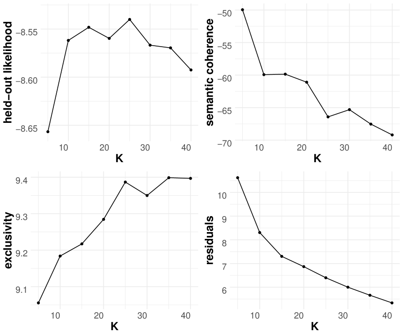
Before fitting the STM, we need to decide on the number of topics, . To do so, we use the following four model evaluation metrics: held-out likelihood, semantic coherence, exclusivity, and residuals. The held-out likelihood approach is based on document completion. The higher the held-out likelihood, the more predictive power the model has on average Wallach et al. (2009). Semantic coherence means that words characterizing a specific topic also appear together in the same documents Mimno et al. (2011). Exclusivity, on the other hand, indicates to which degree words characterizing a given topic only occur in that topic. Finally, the residuals metric, which is based on residual dispersion, indicates a (potentially) insufficiently small value of whenever the residual dispersion is larger than one Taddy (2012).
Figure 1 (left plot) shows these four metrics for a grid of between five and 40 with step size five. Both and seem to be good choices. Taking into account better interpretability for models with fewer topics, we choose .
After fitting the model we label all topics manually using, i.a., the word cloud in Figure 1 (right plot). To obtain an overview of the model output, we can conduct different global-level analyses, such as inspecting global topic proportions or creating a network graph.
5.3 Topic-Metadata Relationships
Moving from global- to document-level, we now visualize relationships between document-level topic proportions and covariates . Specifically, we examine the extent to which German MPs discussed the topic "Climate Protection" over time and in relation to several socioeconomic variables in the respective MP’s electoral district.

To demonstrate the shortcomings of the approach implemented in the stm package, we first apply the estimateEffect function to produce "naïve" estimates for the relationship between estimated topic proportions and document-level covariates. Figure 2 shows the estimated proportion of climate protection over time, peaking during the UN Climate Action Summit 2019 held in September 2019. As can be observed, estimateEffect produces predicted topic proportions outside of . This is due to using an OLS regression, which places no restrictions on the range of the dependent variable.
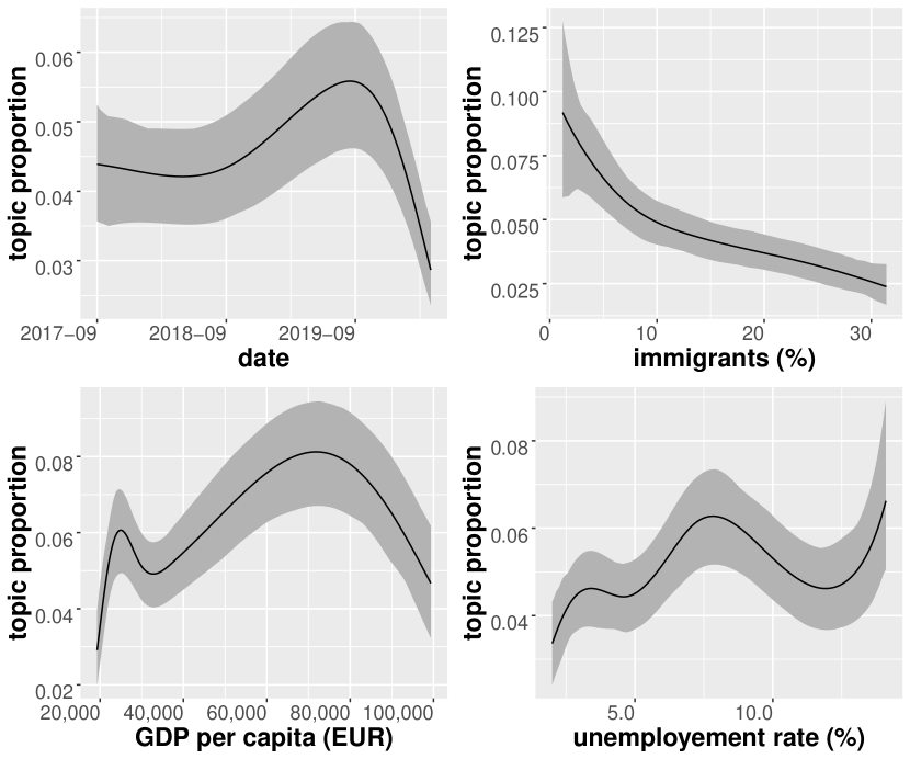
Next, we evaluate the results when replacing the OLS regression by a Beta regression, which assumes the dependent variable to be in . The top left plot of Figure 3 shows that the overall trend over time is similar to the one in Figure 2, yet the range is shifted and no negative values are observed. In addition, Figure 3 depicts the relationship of the climate protection topic with three socioeconomic covariates. On average, the higher the share of immigrants in an electoral district, the less frequently MPs associated with this district tend to discuss climate related subjects. For GDP per capita, we notice an increase until around EUR 70k, but for very high incomes this trend is reversed. The unemployment rate shows an ambiguous relationship, with rather large fluctuations.
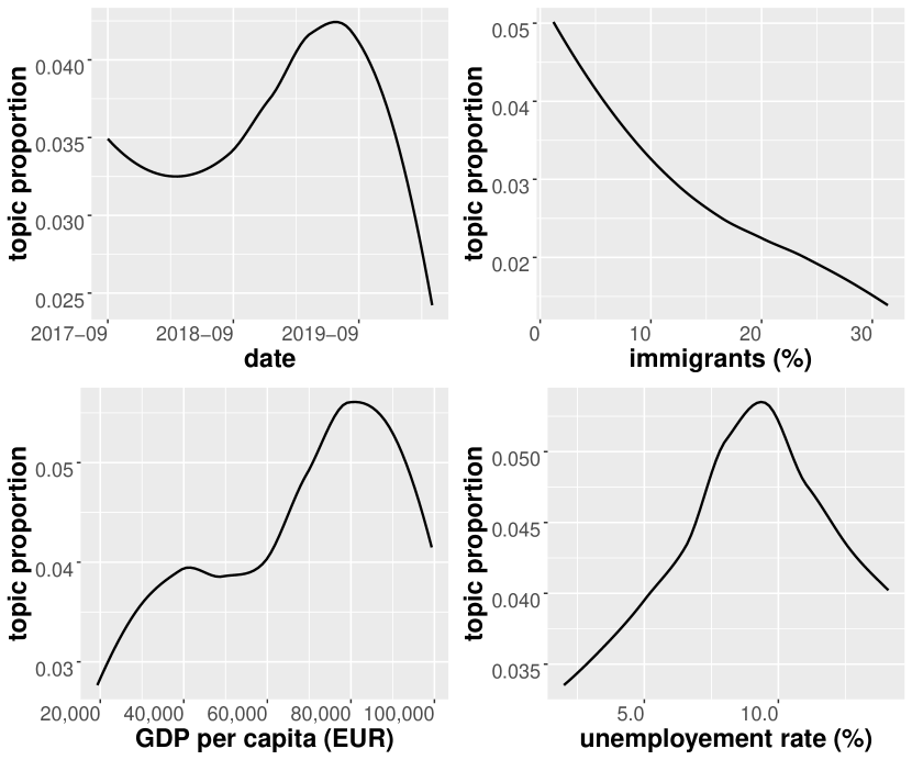
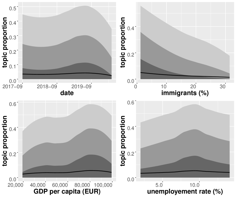
Finally, we display the results from the fully Bayesian approach discussed in Section 4.2. As can be seen in the left plot of Figure 4, the predicted progressions of mean topic proportions at different covariate values are mostly similar to those obtained with the frequentist Beta regression, yet the range is compressed and shifted downwards. In addition to the empirical mean, the right plot of Figure 4 depicts different empirical quantiles of the posterior predictive distribution of topic proportions. Here we can see that topic proportions at different covariate values varies starkly for different MPs. In general, we find that a fully Bayesian approach enables a much more comprehensive exploration of topic-metadata relationships because it allows for displaying the variation of individual topic proportions observed in the data.
6 Conclusion and Outlook
To explore topic-metadata relationships while accounting for the probabilistic nature of topic proportions, the R package stm implements repeated OLS regressions of sampled topic proportions on metadata covariates by using the method of composition. In this paper, we identified shortcomings of and proposed improvements upon this original implementation and applied them to a dataset containing Twitter posts by German MPs. Our methods are equally applicable to other topic models and beyond.
Several possibilities exist to build upon our explorative methods. For instance, to make inference in a Bayesian setting, our approach could be used in combination with MCMC-based methods. If the goal is to make causal inference beyond explorative purposes, one must take into account that the estimation of topic proportions induces additional dependence across documents. Developing methods to identify underlying causal mechanisms is the subject of current research (see e.g. Egami et al., 2018).
References
- Atchison and Shen (1980) J Atchison and Sheng M Shen. 1980. Logistic-normal distributions: Some properties and uses. Biometrika, 67(2):261–272.
- Benoit et al. (2018) Kenneth Benoit, Kohei Watanabe, Haiyan Wang, Paul Nulty, Adam Obeng, Stefan Müller, and Akitaka Matsuo. 2018. quanteda: An r package for the quantitative analysis of textual data. Journal of Open Source Software, 3(30):774.
- Blei et al. (2007) David M Blei, John D Lafferty, et al. 2007. A correlated topic model of science. The Annals of Applied Statistics, 1(1):17–35.
- Blei et al. (2003) David M Blei, Andrew Y Ng, and Michael I Jordan. 2003. Latent dirichlet allocation. Journal of machine Learning research, 3(Jan):993–1022.
- Egami et al. (2018) Naoki Egami, Christian J Fong, Justin Grimmer, Margaret E Roberts, and Brandon M Stewart. 2018. How to make causal inferences using texts. arXiv preprint arXiv:1802.02163.
- Farrell (2016) Justin Farrell. 2016. Corporate funding and ideological polarization about climate change. Proceedings of the National Academy of Sciences, 113(1):92–97.
- Ferrari and Cribari-Neto (2004) Silvia Ferrari and Francisco Cribari-Neto. 2004. Beta regression for modelling rates and proportions. Journal of applied statistics, 31(7):799–815.
- Kim (2017) In Song Kim. 2017. Political cleavages within industry: Firm-level lobbying for trade liberalization. The American Political Science Review, 111(1):1.
- Lucas et al. (2015) Christopher Lucas, Richard A Nielsen, Margaret E Roberts, Brandon M Stewart, Alex Storer, and Dustin Tingley. 2015. Computer-assisted text analysis for comparative politics. Political Analysis, 23(2):254–277.
- Mimno et al. (2011) David Mimno, Hanna M Wallach, Edmund Talley, Miriam Leenders, and Andrew McCallum. 2011. Optimizing semantic coherence in topic models. In Proceedings of the conference on empirical methods in natural language processing, pages 262–272. Association for Computational Linguistics.
- Richardson (2007) Leonard Richardson. 2007. Beautiful soup documentation. April.
- Roberts et al. (2016) Margaret E. Roberts, Brandon M. Stewart, and Edoardo M. Airoldi. 2016. A model of text for experimentation in the social sciences. Journal of the American Statistical Association, 111(515):988–1003.
- Roberts et al. (2019) Margaret E. Roberts, Brandon M. Stewart, and Dustin Tingley. 2019. stm: An R package for structural topic models. Journal of Statistical Software, 91(2):1–40.
- Roesslein (2020) Joshua Roesslein. 2020. Tweepy: Twitter for python! URL: https://github.com/tweepy/tweepy.
- Taddy (2012) Matt Taddy. 2012. On estimation and selection for topic models. In Artificial Intelligence and Statistics, pages 1184–1193.
- Tanner (2012) Martin A Tanner. 2012. Tools for statistical inference. Springer.
- Treier and Jackman (2008) Shawn Treier and Simon Jackman. 2008. Democracy as a latent variable. American Journal of Political Science, 52(1):201–217.
- Wallach et al. (2009) Hanna M Wallach, Iain Murray, Ruslan Salakhutdinov, and David Mimno. 2009. Evaluation methods for topic models. In Proceedings of the 26th annual international conference on machine learning, pages 1105–1112.
- Wang and Blei (2013) Chong Wang and David M Blei. 2013. Variational inference in nonconjugate models. Journal of Machine Learning Research, 14(Apr):1005–1031.