Numerical evidence of a super-universality of the 2D and 3D random quantum Potts models

Abstract

The random $q$-state quantum Potts model is studied on hypercubic lattices in dimensions 2 and 3 using the numerical implementation of the Strong Disorder Renormalization Group introduced by Kovacs and Iglói [Phys. Rev. B 82, 054437 (2010)]. Critical exponents $\nu$, $d_{f}$ and $\psi$ at the Infinite Disorder Fixed Point are estimated by Finite-Size Scaling for several numbers of states $q$ between 2 and 50. When scaling corrections are not taken into account, the estimates of both $d_{f}$ and $\psi$ systematically increase with $q$. It is shown however that $q$-dependent scaling corrections are present and that the exponents are compatible within error bars, or close to each other, when these corrections are taking into account. This provides evidence of the existence of a super-universality of all 2D and 3D random Potts models.

I Introduction

Random quantum ferromagnets are known to undergo a very peculiar phase transition for which quantum fluctuations, that drive the transition in the absence of disorder, are dominated by disorder fluctuations. Thanks to this peculiarity, the properties of the Infinite-Disorder Fixed Point (IDFP) that governs the critical behavior at the transition can be studied using a rather simple real-space renormalization group, introduced by Ma and Dasgupta MaDasgupta , and referred to as Strong Disorder Renormalization Group (SDRG). In the case of the random transverse-field Ising chain (RTIM), Fisher was able to find the asymptotic solution of the flow equations and determine exactly the critical exponents Fisher1 ; Fisher2 ; Monthus1 ; Monthus2 . In particular, the dynamical exponent $z$ is infinite at the fixed point whereas $z=1$ for the pure RTIM. The excitation gap $\Delta E$ displays an essential singularity $\Delta E\sim e^{-aL^{\psi}}$ with the lattice size $L$ where the critical exponent is $\psi=1/2$. The average magnetization follows a power law $\mu\sim L^{d_{f}}$ with a fractal dimension $d_{f}=d-\phi\psi$ and a magnetic critical exponent $\phi$ equals to the golden number $(1+\sqrt{5})/2$. These exponents are expected to be exact. Away from the critical point, in the so-called Griffiths phase, the dynamics is dominated by rare macroscopic clusters of strong (resp. weak) couplings that can order earlier (resp. later) than the rest of the system VojtaReview . As a consequence, the dynamical exponent is larger than $1$ and diverges with the control parameter $\delta$ as $1/|\delta|$ as the IDFP is approached Igloi1 . Finally, the correlation length diverges as $\xi\sim|\delta|^{-\nu}$ with $\nu=2$.

The universality class of the RTIM turned out to be quiet robust: the number of states $q$ of the 1D random quantum Potts model was shown to be an irrelevant parameter in the SDRG flow equations Senthil . Therefore the critical behavior is described by the same IDFP as the RTIM for all values of the number of states $q$, in contrast to what is observed in the classical case where the magnetic critical exponent increases smoothly with $q$ Jacobsen1 ; Chatelain1 ; Jacobsen2 ; Chatelain2 . For a sufficiently strong disorder, the critical behavior of the random $q$-state quantum clock model is also expected to be governed by the same IDFP as the RTIM Senthil ; Carlon1 . The random quantum $N$-color Ashkin-Teller chain, equivalent to $N$ coupled Ising chains, has attracted much attention in the last decade. In the case $N=2$, the phase diagram is qualitatively unchanged by the introduction of disorder Carlon1 . Along the self-dual transition line, the inter-chain coupling is an irrelevant parameter in the SDRG flow equations Goswani . As a consequence, the critical behavior is again the same as the random RTIM whereas exponents vary along the line in the pure case. For strong inter-chain coupling, the transition line splits into two lines, enclosing a new intermediate phase acting as a double-Griffiths phase Vojta3 ; Chatelain3 . Despite the fact that the inter-chain coupling flows towards an infinite value during renormalization, the critical behavior is still in the RTIM universality class along these two lines Vojta3 . In the case $N\geq 3$, the pure Ashkin-Teller chain undergoes a first-order phase transition, as the Potts model with $q\geq 4$, which becomes continuous in presence of disorder Goswani ; Vojta1 ; Vojta2 ; Ibrahim ; Chatelain4 . The critical behavior is in the RTIM universality class at weak inter-chain coupling but seems to be governed by a distinct IDFP at stronger inter-chain coupling Vojta2 .

In this paper, we address the question whether the robustness of the universality class of the RTIM is specific to the 1D case or exists also in higher dimensions. Much less is known about 2D or 3D random quantum ferromagnets. The extension of the SDRG to higher dimensions is trivial but the flow equations are then too complicated for an analytical solution to be found. The numerical implementation of the SDRG rules is complicated by the fact that the topology of the lattice changes during the renormalization. A single site, or cluster, is coupled to a large number of other spins after only a few iterations. Nevertheless, the critical behavior of the 2D RTIM could be shown to be governed by an IDFP Motrunich . An efficient algorithm, allowing for accurate estimates of the critical exponents, was introduced by Kovacs and IglóiKovacs1 ; Kovacs2 . They were able to show that the critical exponents of the random RTIM depend on the dimension of the lattice. Recently, the critical behavior of the 2D quantum Potts model with a quasi-periodic modulation of the couplings was shown to be governed by an infinite quasi-periodicity fixed point, distinct from an IDFP but with an infinite dynamical exponent like an IDFP Agarwal1 ; Agarwal2 . Interestingly, the critical exponents are compatible within error bars for all numbers of states $q\geq 3$. Later on, Kang et al. discussed the IDFP of the random quantum Potts model in light of a mapping onto a discrete gauge model where the size of the gauge group is equal to the number of states $q$ of the Potts model Vasseur . Quantum Monte Carlo simulations were performed for the two-dimensional random quantum Ising model and the 3-state Potts model. The numerical estimates of the critical exponents of the two models are in good agreement, providing evidence of an independence on $q$ and the super-universality of the IDFP in two dimensions.

In this work, the $q$-state random quantum Potts model is considered in two and three dimensions. Since in the classical 2D random Potts model, the magnetic critical exponent increases slowly with $q$, we considered number of states up to $q=50$. Critical exponents are estimated numerically using the Kovacs-Iglói algorithm. In the first section of this paper, the model and the algorithm are presented. The determination of the location of the critical points is detailed in section III. The correlation length exponent $\nu$ is extracted from the statistics of the pseudo-critical points. In section IV, the magnetic fractal dimension $d_{f}$ is estimated from the Finite-Size Scaling of the average magnetic moment. In section V, the exponent $\psi$ is estimated from the analysis of the average energy gap. Conclusions follow.

II Potts model and SDRG algorithm

II.1 The random quantum Potts model

The $q$-state quantum Potts model is defined on a lattice $\Lambda=(V,E)$ by the Hamiltonian Stefen ; Solyom

$$H_{\rm Potts}=-\sum_{(i,j)\in E}J_{ij}D_{i,j}-\frac{1}{q}\sum_{i\in V}h_{i}M_{i}$$ (1)

acting on the Hilbert space spanned by the states $\bigotimes_{i\in V}\ket{n_{i}}$ with $n_{i}=0,\ldots,q-1$. The first sum extends over the set $E$ of edges of the lattice $\Lambda$ and the matrix elements of the diagonal operator $D_{i,j}$ vanish unless $n_{i}=n_{j}$, in which case they are equal to 1. A representation of this operator in terms of local operators is given by

$$D_{i,j}={1\over q}\sum_{n=0}^{q-1}\Omega_{i}^{n}\Omega_{j}^{-n}$$ (2)

where $\Omega_{i}={\mathbbm{1}}^{\otimes i-1}\otimes\Omega\otimes{\mathbbm{1}}^{\otimes N-i}$ ($N$ is the number of sites of the lattice) and $\Omega$ is a diagonal $q\times q$ matrix whose diagonal elements are $\omega^{n}$ with $\omega=e^{2i\pi/q}$. In the pure case, i.e. $J_{ij}=J>0$, the first term of the Hamiltonian favors a ferromagnetic ordering of the spins, i.e. $n_{i}=n$ $\forall i$. The second sum of the Hamiltonian (1) extends over the set $V$ of sites of the lattice $\Lambda$ and $M_{i}={\mathbbm{1}}^{\otimes i-1}\otimes M\otimes{\mathbbm{1}}^{\otimes N-i}$ with $M$ the $q\times q$ matrix whose elements are all equal to 1. In the pure case, $h_{i}=h$, the second term of the Hamiltonian destroys the ferromagnetic ordering and is associated to quantum fluctuations. When $q=2$, the Potts model is equivalent to the RTIM whose Hamiltonian takes the simpler form

$$H_{\rm Ising}=-\sum_{(i,j)\in E}J_{ij}\sigma_{i}^{z}\sigma_{j}^{z}-\sum_{i\in V}h_{i}\sigma_{i}^{x}$$ (3)

where $\sigma_{i}^{x,z}$ are Pauli matrices acting on the site $i$ of the lattice. In the one-dimensional case, only the Ising model is exactly solvable when $J_{ij}=J$ and $h_{i}=h$. Duality arguments predict that the transition point is located at $J=h$ for any number of states $q$. The pure Potts chain undergoes a second-order phase transition when $q\leq q_{c}(1)=4$ and a first-order transition when $q>q_{c}(1)$. At higher dimensions $d>1$, the transition point is not known exactly. The number of states $q_{c}(d)$ separating the regime of first and second-order phase transition is also not known exactly for $d>1$.

In the following, the Potts model with quenched disorder is considered. The exchange couplings $J_{ij}$ and the transverse fields $h_{i}$ are independent random variables distributed according to the distributions $P_{0}(J_{ij})$ and $Q_{0}(h_{i})$. As mentioned in the introduction, the critical exponents of the random RTIM ($q=2$) has been determined exactly by Fisher. In dimensions $d=2,3,$ and 4, they were estimated numerically by Kovacs and Iglói. In the following, the RTIM will be used as a test bed for our implementation of the SDRG algorithm and for the analysis of the numerical data. In the regime $q>q_{c}(d)$, the first-order phase transition of the pure Potts model is expected to be rounded by disorder and turned into a continuous transition, as first discussed by Goswani et al. Goswani . A rigorous proof was later given that an infinitesimal amount of disorder is sufficient to round any first-order phase transitions in quantum systems in dimensions $d\leq 2$ Aizenman1 ; Aizenman2 . For $d>2$, the first-order phase transition may survive at weak disorder, as in the classical case for $d\geq 3$, for example in the random 3D 4-state classical Potts model Chatelain5 ; Chatelain6 .

In this work, several probability distributions were considered. The uniform distribution

$$P_{0}(J_{ij})=\Theta(J_{ij})\Theta(1-J_{ij}),$$ (4)

where $\Theta$ is the Heaviside function, for the exchange couplings and

$$Q_{0}(h_{i})=\frac{1}{h_{\rm max}}\Theta(h_{i})\Theta(h_{\rm max}-h_{i})$$ (5)

for the transverse fields. The Potts model is in the ferromagnetic phase for a sufficiently small parameter $\theta=\log h_{\rm max}$ and in the paramagnetic phase for large $\theta$. The distributions (4) and (5) are referred to as weak disorder in the following. These distributions are expected to evolve along the RG flow and become broader and broader. Because the distributions $P_{0}$ and $Q_{0}$ are far from the distributions at the IDFP, corrections to scaling are expected for small lattice sizes and therefore small numbers of RG steps. To minimize these corrections, pow-law distributions

$$P_{0}(J_{ij})\sim J_{ij}^{-\Delta},\quad(0<J_{ij}<1)$$

$$Q_{0}(h_{i})\sim h_{i}^{-\Delta},\quad(0<h_{i}<h_{\rm max})$$ (6)

were also considered for several numbers of states $q$ of the Potts model. The value $\Delta=2/3$ is referred to as a medium disorder and $\Delta=4/5$ as a strong disorder.

II.2 SDRG algorithm

The Strong Disorder Renormalization Group (SDRG) is a real-space decimation scheme where the strongest coupling $\Omega=\max(\{J_{ij}\},\{h_{i}\})$ is decimated at each iteration Fisher1 ; Fisher2 ; Monthus1 . The case of the RTIM is discussed first. If the strongest coupling is an exchange coupling, say $\Omega=J_{ij}$, the two spins $i$ and $j$ are merged into a new effective cluster whose magnetic moment $\mu^{\prime}=\mu_{i}+\mu_{j}$ is the sum of the moments $\mu_{i}$ and $\mu_{j}$ of the two spins $i$ and $j$. Second-order perturbation theory shows that this new cluster is coupled to an effective transverse field $h^{\prime}=\frac{h_{i}h_{j}}{J_{ij}}$ and to any other spin $k\neq i,j$ by an exchange coupling $J_{ik}^{\prime}=J_{ik}+J_{jk}$. If the strongest coupling $\Omega$ is a transverse field, say $h_{i}$, the spin $i$ is decimated. An effective coupling is induced between all pairs of spins $k$ and $l$ that were both coupled to site $i$. To second order in perturbation theory, this effective coupling is $J^{\prime}_{kl}=J_{kl}+\frac{J_{ik}J_{il}}{h_{i}}$. As this scheme is iterated, the probability distributions $P(J)$ and $Q(h)$ of the couplings become broader and broader so that second-order perturbation theory is expected to become exact at the IDFP. The sum rule can then be replaced by a maximum rule: at the IDFP, it is sufficient to write the exchange coupling of a spin $k$ with the new effective cluster at site $i$ as the maximum $J_{ik}^{\prime}=\max(J_{ik},J_{jk})$ instead of the sum. Similarly, the effective exchange coupling $J_{kl}^{\prime}$ induced by the decimation of the site $i$ can be simplified as $J^{\prime}_{kl}=\max(J_{kl},\frac{J_{ik}J_{il}}{h_{i}})$. For the Potts model, the SDRG rules are shown to be Senthil

$$h^{\prime}=\frac{h_{i}h_{j}}{\kappa J_{ij}},\quad J^{\prime}_{kl}=J_{kl}+\frac{J_{ik}J_{il}}{\kappa h_{i}}$$ (7)

where $\kappa=q/2$. These rules are the same for any dimension $d$ of the lattice. However, the main difficulty in implementing them numerically when $d>1$ comes from the increasing number of couplings $J_{ij}$ that are generated at each decimation. Finding the largest coupling requires more and more CPU time and even storing all the couplings restricts the application to small lattice sizes. A crucial simplification was introduced by Kovacs and Iglói Kovacs1 ; Kovacs2 . They showed that many couplings are actually irrelevant at the IDFP. The resulting algorithm and the details of our implementation for the Potts model are discussed in the following.

The Hamiltonian can be seen as a weighted graph. A weight

$$r_{i}=-\ln h_{i}$$ (8)

is attached to each node $i$ and an edge with a distance

$$d_{ij}=d_{ji}=-\ln J_{ij}$$ (9)

is defined between each pair $(i,j)$ of nodes of the graph for which $J_{ij}\neq 0$. With the above definitions, the SDRG rules become:

• If $r_{i}$ is the global minimum, equivalently if $h_{i}$ is the global maximum, then the node $i$ is removed. For all pairs of sites $(k,l)$ connected to $i$, i.e. such that $J_{ik},J_{il}\neq 0$, the distance $d_{kl}$ is updated as

  $$d_{kl}^{\prime}=\min(d_{kl},d_{ki}+d_{il}-r_{i}+\ln\kappa)$$ (10)

  which is equivalent to (7) when replacing the sum rule by the maximum rule.

• If $d_{ij}$ is the global minimum, or equivalently if $J_{ij}$ is the global maximum, then the two nodes $i$ and $j$ are merged into a single node $i$ whose weight is

  $$r_{i}^{\prime}=r_{i}+r_{j}-d_{ij}+\ln\kappa$$ (11)

  which is again equivalent to (7). For each node $k$ previously connected to both $i$ and $j$, i.e. $J_{ik},J_{jk}\neq 0$, the distance to the new site $i$ is updated as $d_{ki}^{\prime}=\min(d_{ik},d_{jk})$.

Several improvements can be implemented. First, instead of removing the node $i$ when the spin is decimated ($\Omega=h_{i}$), it is set as inactive. The definition (9) of the distances $d_{ij}$ are modified to

$$d_{ij}=d_{ji}=-\ln J_{ij}+\frac{l_{i}}{2}\ln(\kappa h_{i})+\frac{l_{j}}{2}\ln(\kappa h_{j})$$ (12)

where $l_{i}$ is the activation status of the node $i$ which takes the value $l_{i}=0$ when the node has not been decimated yet (the node is then said to be active) and 1 otherwise (the node is inactive). By setting the node $i$ as inactive instead of removing it when $\Omega=h_{i}$, it is not necessary anymore to add new edges associated to the effective couplings that are generated by second order perturbation theory. Instead, the exchange coupling between two active sites $k$ and $l$ is computed on the fly when necessary as $J_{kl}=e^{-\delta_{kl}}$ where $\delta_{kl}$ is the shortest distance of all paths of the graph joining sites $k$ and $l$ and going through inactive sites only. If no path connects $k$ and $l$ then $J_{kl}=0$. The condition of the shortest distance is equivalent to the maximum rule and the SDRG rule is recovered. Indeed, when the site $i$ is decimated, $\delta_{kl}=d_{ki}+d_{il}=-\ln J_{ki}+\ln(\kappa h_{i})-\ln J_{il}$ so that the effective exchange coupling is $J_{kl}^{\prime}=e^{-\delta_{kl}}={J_{ki}J_{il}\over\kappa h_{i}}$ as expected. The advantage of this implementation is that the number of edges does not grow during site decimation. Inactive sites are removed during edge decimation: if $\Omega=\delta_{ij}$, sites $i$ and $j$ are merged into a new cluster on site, say $i$. All inactive sites $k$ belonging to the shortest path between sites $i$ and $j$ can now be removed and all edges $d_{kl}$ are added to $d_{il}$ using the minimum rule $d_{il}^{\prime}=\min(\delta_{il},d_{ik}+d_{kl})$.

The computation of the shortest distance $\delta_{kl}$ between two sites can be time-consuming. Hopefully, the shortest distance can be determined efficiently using Dijkstra algorithm Djikstra . Note that Dijkstra algorithm requires the distances to be positive. The distance $d_{ij}=-\ln J_{ij}$ between two active sites can be made positive by initially choosing all exchange couplings $J_{ij}$ smaller or equal to 1. When $\kappa\geq 1$, the SDRG rules imply that $J_{ij}^{\prime}\leq 1$ after renormalization. If the site $j$ is inactive while $i$ is active, the distance $d_{ij}=-\ln J_{ij}+{1\over 2}\ln(\kappa h_{j})$ is positive too because the decimation of the node $j$ has been possible only if $h_{j}>J_{ij}$. It follows that $-\ln J_{ij}+{1\over 2}\ln h_{j}+{1\over 2}\ln\kappa>-{1\over 2}\ln J_{ij}+{1\over 2}\ln\kappa\geq 0$ which completes the proof that $d_{ij}\geq 0$ when $\kappa\geq 1$ and $J_{ij}\leq 1$. However, the distance $d_{ij}$ can be negative when the two sites are inactive. When it is the case, any path reaching site $i$ will then go to site $j$. As a consequence, for any neighbor $k\neq i$ of site $j$, one can create or update the distance between $i$ and $k$ as $d_{ik}^{\prime}=\min(d_{ik},d_{ij}+d_{jk})$ and remove the site $j$ and all edges $d_{jk}$.

The second improvement concerns the choice of the next coupling to be renormalized. It is not necessary to find the global minimum. Finding and decimating a local minimum is sufficient if the local minimum is defined as:

• $r_{i}$ is a local minimum if $r_{i}<\delta_{ik}$ for all $k$ such that there exists at least one path between $i$ and $k$. No edge involving the node $i$ can therefore be decimated before the node $i$.

• $\delta_{ij}$ is a local minimum if $\delta_{ij}<r_{i},r_{j}$ and if $\delta_{ij}<\delta_{ik}$ or $\delta_{ij}<\delta_{jk}$ when there exists at least one path between $i$ or $j$ and $k$.

These definitions ensure that a local minimum remains a local minimum when any another node or edge is decimated first. The proof follows from the fact that:

• if the node $j$ is decimated first, which implies that $r_{j}<\delta_{jk}$ for all sites $k$ for which there exists at least one path joining $j$ and $k$, the site $j$ is set inactive. The distances between the site $j$ and its neighbors $l$ are updated to $d_{jl}^{\prime}=d_{jl}-{1\over 2}r_{j}+{1\over 2}\ln\kappa$. The shortest distance $\delta_{ik}$ is therefore unchanged if the shortest path does not go through the site $j$ and becomes $\delta_{ik}^{\prime}=\delta_{ij}+\delta_{jk}-r_{j}+\ln\kappa$ otherwise. Since $r_{j}<\delta_{jk}$ and $r_{i}<\delta_{ij}$ if $r_{i}$ is a local minimum, the new value $\delta_{ik}^{\prime}$ is necessarily larger than $r_{i}$. $r_{i}$ remains therefore a local minimum.

• if the edge $\delta_{jk}$ is decimated first, the distance between a site $i\neq j,k$ and the new site, say $j$, is updated to the value $\delta_{ij}^{\prime}=\min(\delta_{ij},\delta_{ik})$. If $r_{i}$ is a local minimum, the condition $r_{i}<\delta_{ij},\delta_{ik}$ holds. It follows that $r_{i}<\delta_{ij}^{\prime}$ and therefore, $r_{i}$ remains a local minimum.

Similarly, the distance $\delta_{ij}$ remains a local minimum in the following situations:

• if the node $k$ is decimated first, which implies that $r_{k}<\delta_{kl}$, for all sites $l$ for which there exists at least one path joining $k$ and $l$, the shortest distance $\delta_{ij}$ is unchanged if the shortest path does not go through the site $k$ and becomes $\delta_{ij}^{\prime}=\delta_{ik}+\delta_{jk}-r_{k}+\ln\kappa$ otherwise. Since $r_{k}<\delta_{ik},\delta_{jk}$ and $\delta_{ij}<\delta_{ik}$ or $\delta_{ij}<\delta_{jk}$ if $\delta_{ij}$ is a local minimum, the effective distance $\delta_{ij}^{\prime}=\delta_{ik}+\delta_{jk}-r_{k}+\ln\kappa$ is larger than $\delta_{ij}$. The latter will therefore remain a local minimum.

• if the edge $\delta_{kl}$ is decimated first, the distance between a site $i\neq k,l$ and the new site, say $k$, is updated to the value $\delta_{ik}^{\prime}=\min(\delta_{ik},\delta_{il})$. If the $\delta_{ij}$ was a local minimum with the condition $\delta_{ij}<\delta_{ik},\delta_{il}$ then $\delta_{ij}<\delta_{ik}^{\prime}$ and therefore $\delta_{ij}$ remains a local minimum.

• if the edge $\delta_{jk}$ is decimated first, the weight of the new node $j$ becomes $r^{\prime}_{j}=r_{j}+r_{k}-\delta_{jk}+\ln\kappa$. Since $\delta_{jk}<r_{k}$, the inequality $r_{j}^{\prime}>r_{j}$ holds. Therefore, if $\delta_{ij}$ is a local minimum, the condition $\delta_{ij}<r_{j}$ is preserved when the edge $\delta_{jk}$ is decimated. Distances will also be modified. In particular, $\delta_{ij}$ will be replaced by $\min(\delta_{ij},\delta_{ik})$. Since $\delta_{jk}$ was decimated first, $\delta_{jk}<\delta_{ij}$ so the condition $\delta_{ij}<\delta_{il}$ for all $l$ for which there exists a path between $i$ and $l$, should hold for $\delta_{ij}$ to be local minimum. In particular, $\delta_{ij}<\delta_{ik}$ and therefore the value of $\delta_{ij}$ will not be modified by the decimation of $\delta_{jk}$. For $l\neq k$, $\delta_{il}$ is unchanged because a path joining $i$ and $l$ can only go through inactive sites, so neither $j$ or $k$. In conclusion, $\delta_{ij}$ will remain a local minimum after the decimation of $\delta_{jk}$.

Local minimum can be decimated in any order. One can check that the same decimations as in the original SDRG will take place. Only the order differs. A lot of computation time is saved in looking for local minimum instead of the global one. The drawback of this method is that the renormalization flow being modified, one cannot study anymore the evolution of the total magnetic moment or the number of sites as a function of $\Omega$. Instead, the critical exponents should be estimated from the behavior of the magnetic moment or the transverse field of the last decimated site in the original SDRG. In our implementation, this site could have been decimated anywhere in the RG flow so one has to keep track of the smallest transverse field at each decimation.

III Critical point

The random $q$-state Potts model is studied on 2D and 3D hypercubic lattices with the above-detailed algorithm. The data have been averaged over more than $3000$ disordered configurations for the largest lattice sizes and up to $10^{6}$ for the smallest ones. These numbers were chosen in order to achieve a good convergence of average quantities. On Fig. 1, the average magnetic moment of the last decimated cluster during the original SDRG is plotted versus the number of samples in the case of the 3D 10-state Potts model. Rare events with a large contribution, usually expected in random systems, do not seem to have any influence on the plateau reached by the average magnetic moment. As can be seen on Fig. 1 in the case of the 3D 10-state Potts model, the relative fluctuations of $\bar{\mu}$ are, in the worst case $L=160$, of order ${\Delta\mu\over\bar{\mu}}\simeq 1/150<1\%$. The estimation of the error as $\sqrt{{\rm Var}\ \!\mu/N}$, where ${\rm Var}\ \!\mu$ is the variance of the data and $N$ the number of disordered configurations, leads to a relative error of $0.6\%$ for the 3D 10-state Potts model at $L=160$. For the critical exponents that will be estimated in the following, the error due to the finite number of disordered configurations is a small contribution compared to the error coming from the fits.

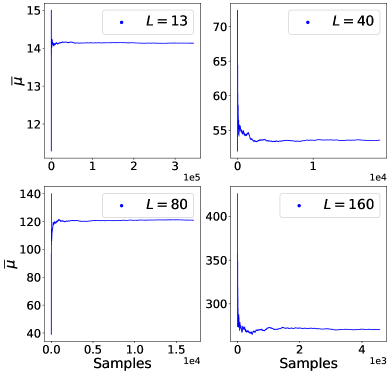
Figure 1: Average value of the magnetic moment $\mu$ of the last decimated cluster of the 3D $q=10$-Potts model with respect to the number of disordered samples. The four graphs correspond to different lattice sizes $L$. Note that the number of samples given on the $x$-axis has to be multiplied by $10^{5}$ ($L=13$, top left), $10^{4}$ ($L=40$, top right), $10^{4}$ ($L=80$, bottom left) and $10^{3}$ ($L=160$, bottom right).

A pseudo-critical point $\theta_{c}^{i}(L)\equiv\ln h_{c}^{i}(L)$ is determined for each disordered sample $i$ using the doubling method Kovacs1 ; Kovacs2 . Two identical replicas of the same system, i.e. with the same exchange couplings and transverse fields, are glued together with some specific boundary conditions. When the SDRG procedure is applied to both the joint system of size $2L$ and the initial one of size $L$, the ratio $\mu(2L)/\mu(L)$ of the magnetic moments of the last decimated cluster is expected to show a jump at the pseudo-critical point. In the paramagnetic phase, $\theta>\theta_{c}^{i}(L)$, the decimated cluster is located in one of the two replicas and $\mu(2L)=\mu(L)$. In contrast, in the ferromagnetic phase, $\theta<\theta_{c}^{i}(L)$, the last decimated cluster spans the two replicas and $\mu(2L)=2\mu(L)$. In practise, the system is considered to be in the ferromagnetic phase if the last decimated cluster contains the same sites in both replicas. To locate the pseudo-critical point, an interval $[\theta_{1},\theta_{2}]$ is manually chosen and is refined by performing additional simulations at $\theta={1\over 2}(\theta_{1}+\theta_{2})$ until the targeted accuracy $\epsilon=|\theta_{2}-\theta_{1}|$ is reached. In the following, the accuracy on the pseudo-critical point $\theta_{c}^{i}(L)$ is $10^{-5}$.

As the lattice size is increased, the pseudo-critical points $\theta_{c}^{i}(L)$ are expected to converge to the critical point $\theta_{c}$ of the infinite system as

$$|\theta_{c}^{i}(L)-\theta_{c}|\sim L^{-1/\nu}$$ (13)

where $\nu$ is the correlation length exponent. As a consequence, the probability distribution of the pseudo-critical points $\theta_{c}^{i}(L)$ should be independent of the lattice size $L$ when plotted with respect to the rescaled distance to the critical point $u=L^{1/\nu}|\theta_{c}^{i}(L)-\theta_{c}|/\theta_{c}$. This plot is shown on Fig. 2 for the 2D and 3D 10-state Potts models. As expected, all points fall nicely on the same curve when the two parameters $\theta_{c}$ and $\nu$ are appropriately chosen. To determine the values leading to the best collapse of the probability distributions $P_{L}(u)$ for different lattice sizes $L$, the following cost function

$$\sigma=\frac{1}{u_{\rm max}-u_{\rm min}}\int_{u_{\rm min}}^{u_{\rm max}}\sum_{L}\Big{[}P_{L}(u)-{1\over N_{L}}\sum_{L}P_{L}(u)\Big{]}^{2}du$$ (14)

was numerically minimized using Powell method. Only $N_{L}=4$ lattice sizes were considered. $u_{\rm min}$ and $u_{\rm max}$ are the smallest and largest values of $u$ in the dataset. The optimal values of the parameters $\theta_{c}$ and $\nu$ are collected in Table 1 for the 2D and 3D Potts models. The estimates of the correlation length exponent $\nu$ are compatible within error bars for the 2D (resp. 3D) Potts model, independently of the number of states $q$ of the Potts model.

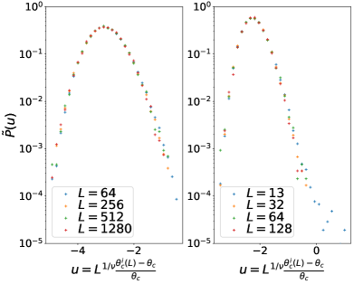
Figure 2: Probability distribution $P(u)$ of the rescaled distance $u=L^{1/\nu}(\theta_{c}^{i}(L)-\theta_{c})/\theta_{c}$ to the critical point for the four largest lattice sizes that were considered in the minimization of the cost function Eq. 14. On the left, the data for the $2D$ 10-state Potts model are plotted with the parameters $\nu=1.2594$ and $\theta_{c}=1.457$. On the right, the data for the $3D$ 10-state Potts model are plotted with the parameters $\nu=1.008$, $\theta_{c}=2.332$.

Table 1: Estimates of the critical point $\theta_{c}$ and correlation length exponent $\nu$ of the 2D and 3D random Potts models. $\theta_{c}$ and $\nu$ were obtained by imposing the collapse of the probability distribution $P(u)$.

2D	$q=2$	$3$	$5$	$10$	$20$	$50$
$\theta_{c}$	1.678(1)	1.563(1)	1.495(1)	1.457(1)	1.442(1)	1.435(1)
$\nu$	1.25(2)	1.24(2)	1.25(2)	1.26(2)	1.24(2)	1.25(2)
3D	$q=2$	$3$	$5$	$10$	$20$	$50$
$\theta_{c}$	2.532(1)	2.420(1)	2.359(1)	2.332(1)	2.325(1)	2.327(1)
$\nu$	1.01(1)	1.004(10)	1.001(10)	1.008(10)	1.004(10)	1.005(10)

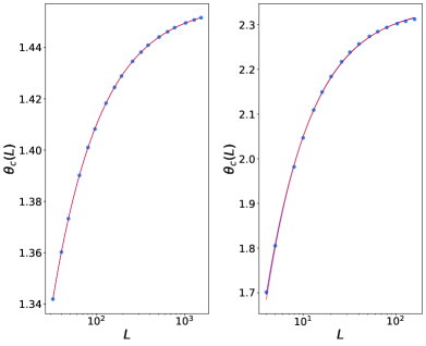
Figure 3: Average critical point $\bar{\theta}_{c}(L)$ versus the lattice size $L$ of the 2D (left) and 3D (right) $q=10$ Potts model. The blue curve corresponds to a simple fit without any correction while the red curve corresponds to a fit with an algebraic correction. They can be distinguished on the figure for small $L$ in the 3D case.

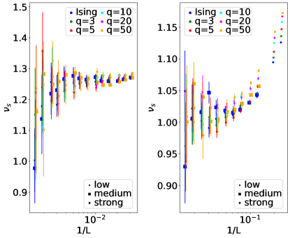
Figure 4: Effective exponent $\nu_{s}$ versus the smallest lattice size $L_{\rm min}$ entering into the fit for the 2D (left) and 3D (right) Potts models. The different colors correspond to different numbers of states $q$ of the Potts model. The different symbols correspond to different initial probability distributions of the couplings.

The correlation length exponent $\nu$ was also estimated by performing a non-linear fit of the shift of the average pseudo-critical point $\bar{\theta}_{c}(L)$ as $|\bar{\theta}_{c}(L)-\theta_{c}|=aL^{-1/\nu_{s}}$ where $\theta_{c}$, $a$ and $\nu_{s}$ are free parameters. The notation $\nu_{s}$ is used here to distinguish this estimate from the one obtained from the collapse of the probability distribution. The average pseudo-critical point is plotted on Fig. 3 for the 2D and 3D 10-state Potts models. For the other values of the number of states $q$ that were considered ($q=3,5,20$ and 50), the curves are similar. We tried to take into account possible algebraic scaling corrections by performing a non-linear fit of the data with the function $|\bar{\theta}_{c}(L)-\theta_{c}|=aL^{-1/\nu_{s}}\big{(}1+bL^{-\omega}\big{)}$ where now $\theta_{c}$, $a$, $\nu_{s}$, $b$ and $\omega$ are free parameters. Due to the small number of degrees of freedom, this fit turned out to be quite unstable, different fitting algorithms leading to incompatible values. An indirect method was therefore applied to estimate the true exponent $\nu_{s}$: the non-linear fit $|\bar{\theta}_{c}(L)-\theta_{c}|=aL^{-1/\nu_{s}}$ was performed on various ranges of lattice sizes. A $L_{\rm min}$-dependent effective exponent $\nu_{s}(L_{\rm min})$ is then estimated by a non-linear fit restricted to the lattice sizes $L\geq L_{\rm min}$. As can be seen in Fig. 4 for $q=10$, this effective exponent is relatively stable for small $L_{\rm min}$ but displays large fluctuations at large $L_{\rm min}$ because of a number of degrees of freedom of the fit becoming smaller and smaller. The error bars on $\nu_{s}(L_{\rm min})$ correspond to the standard deviation of the fit. They do not take into account the accuracy on $\theta_{c}(L)$, equal to $10^{-5}$, which leads to a much smaller contribution (or order ${\cal O}(10^{-5})$) to the error on $\nu_{s}(L_{\rm min})$. In the 2D case, the effective exponents do not vary significantly with $L_{\rm min}$, which means that scaling corrections are weak. The exponents for different numbers of states $q$ of the Potts model are compatible within error bars. In contrast, for the 3D Potts model, the influence of a correction is clearly seen as a stronger dependence of the effective exponents on $1/L_{\rm min}$. For small $L_{\rm min}$, the exponents $\nu_{s}$ of the $q$-state Potts models increase with $q$ and are fully incompatible. As $L_{\rm min}$ is increased, the exponents take smaller values and their dispersion shrinks, although their fluctuations increase. For large $L_{\rm min}$, a plateau seems to be reached around $\nu_{s}\simeq 1.00$.

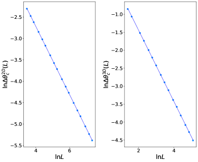
Figure 5: Standard deviation of the critical point $\Delta\theta_{c}(L)$ versus the lattice size $L$ of the 2D (left) and 3D (right) $q=10$ Potts models. The blue curve is a linear fit.

Figure 6: Effective exponent $\nu_{w}$ versus the smallest lattice size $L_{\rm min}$ entering into the fit for the 2D (left) and 3D (right) Potts models. The different colors correspond to different numbers of states $q$ of the Potts model. The different symbols correspond to different initial probability distributions of the couplings.

Finally, a third estimate of the correlation exponent $\nu$ was obtained from the standard deviation $\Delta\theta_{c}(L)=\sqrt{\overline{\theta_{c}^{2}(L)}-(\overline{\theta_{c}(L)})^{2}}$. The latter is expected to scale as $L^{-1/\nu}$ with the lattice size. A linear fit (in log-log scale) with only two free parameters is therefore sufficient in this case. To distinguish from the previous estimates, the exponent estimated from the standard deviation $\Delta\theta_{c}(L)$ will be denoted as $\nu_{w}$ in the following. An example for the 2D and 3D 10-state Potts model is presented in Fig. 5. The presence of scaling corrections is observed in the 3D case. Effective exponents $\nu_{w}(L_{\rm min})$, estimated by restricting the fit to lattice sizes $L\geq L_{\rm min}$, are shown on Fig. 6. In the 2D case, the effective exponents $\nu_{w}$ are spread around the value $1.25$ for small $L_{\rm min}$, i.e. for fits over all or most of the lattice sizes, and are compatible within error bars. However, different evolutions are observed as $L_{\rm min}$ is increased. Some exponents increase while others decrease. Note that the effective exponents $\nu_{w}(L_{\rm min})$ for a given number of states $q$ and a given initial distribution of the couplings are highly correlated because they were computed with fits over the same set of data. We were not able to identify a correlation between these different behaviors and the number of states $q$ of the Potts model or the strength of disorder in the initial distribution of the couplings. These different evolutions at large $L_{\rm min}$ are therefore probably statistical fluctuations. The 3D case is hopefully a bit clearer. The effective exponents decrease with $L_{\rm min}$ and are compatible within error bars or close to the value $\nu_{w}\simeq 0.98$ in the limit $1/L_{\rm min}\rightarrow 0$. We have no reason to believe that different Potts models belong to different universality class.

From the effective exponents at large $L_{\rm min}$, a rough estimate of the correlation lengths exponents can be inferred: $\nu_{s}\simeq 1.25(6)$ and $\nu_{w}\simeq 1.25(3)$ in the 2D case, and $\nu_{s}\simeq 1.01(5)$ and $\nu_{w}\simeq 0.985(10)$ in the 3D case. These estimates are compatible within error bars with the values of the literature for the Ising model: $1.24(2)$ in the 2D case Kovacs1 and $\nu_{s}=0.99(2)$ and $\nu_{w}=0.97(5)$ in the 3D case Kovacs2 .

IV Magnetic exponent

The computation of the magnetic moment $\mu$ of the last decimated cluster has revealed unexpected difficulties: for a given sample, $\mu$ often displays a jump at the pseudo-critical point. This jump is rare and quite small for the Ising model but more frequent and larger when the number of states $q$ of the Potts model is increased. Since the pseudo-critical points $\theta_{c}^{i}(L)$ of each sample was estimated with an accuracy of $10^{-5}$, the estimates of the magnetic moment take randomly the value at the left or at the right of the jump. The average magnetic moment is therefore equal to the mean of the values at the left and at the right of the jump. We have checked that the relative width of this jump decreases with the lattice size $L$. For power-law initial distributions of the couplings (6), broader than the uniform one, smaller jumps were observed.

The fractal dimension $d_{f}$ of magnetization is estimated from the Finite-Size Scaling

$$\bar{\mu}\sim L^{d_{f}}.$$ (15)

of the average magnetic moment $\bar{\mu}$ of the last decimated cluster at the pseudo-critical point $\theta_{c}^{i}(L)$ of each sample. The average magnetic moment $\bar{\mu}$ is plotted in Fig. 7 for the 2D and 3D 10-state Potts models. For the other values of the number of states $q$ that were considered ($q=3,5,20$ and 50), the curves are similar. The blue curve is the result of a linear fit of $\ln\bar{\mu}$ with $\ln L$. In both the 2D and 3D cases, the estimated fractal dimensions $d_{f}$ are incompatible and systematically increase with the number of states $q$ of the Potts model. A non-linear fit with an algebraic correction, $\bar{\mu}=aL^{d_{f}}\big{(}1+bL^{-\omega}\big{)}$ was performed but none of the algorithms that were used gave a stable estimate of $d_{f}$. To nevertheless take into account possible $q$-dependent scaling corrections, the fit was performed on various ranges of lattice sizes. As for the correlation-length exponent, a $L_{\rm min}$-dependent effective exponent $d_{f}(L_{\rm min})$ is estimated by a fit restricted to the lattice sizes $L\geq L_{\rm min}$. This effective exponent is shown in Fig. 8. The influence of a correction is clearly seen as a dependence with $1/L_{\rm min}$. In the case of the 2D random Potts model, the fractal dimension $d_{f}$ increases with $L_{\rm min}$ for the Ising model, is roughly stable for $q=3$ and decreases for $q\geq 4$. As a consequence, the spreading of the effective exponents $d_{f}(L_{\rm min})$ decreases with $L_{\rm min}$. Even though all exponents are not compatible within error bars, the super-universality of the 2D random Potts models seems much more plausible than without taking into account scaling corrections. In the case of the 3D random Potts model, the scenario is similar. When scaling corrections are not taken into account, the estimates of the fractal dimensions $d_{f}$ are fully incompatible. As $L_{\rm min}$ is increased, the spreading of the effective exponents $d_{f}(L_{\rm min})$ shrinks and the fractal dimensions are finally compatible with the value $1.155$. Two exceptions can be noticed: the Ising model and the $q=50$ Potts model with weak disorder, whose exponents are still far from $1.155$ at large $L_{\rm min}$. However, at medium disorder, the exponents are remarkably closer to others and are compatible with $1.155$ at large $L_{\rm min}$.

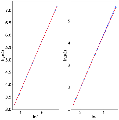
Figure 7: Average magnetic moment of the last decimated cluster $\bar{\mu}(L)$ versus the lattice size $L$ of the 2D (left) and 3D (right) $q=10$ Potts model. In the 3D case, the light blue curve corresponds to a simple fit without any correction while the red curve corresponds to a fit with an algebraic correction.

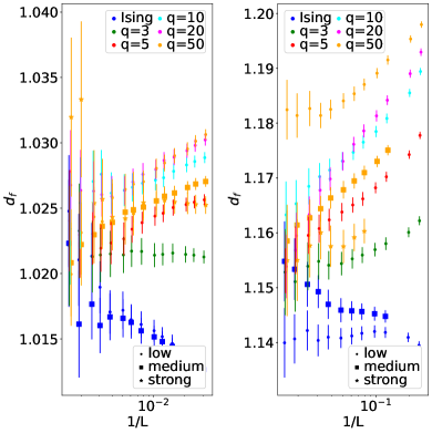
Figure 8: Effective exponent $d_{f}$ versus the smallest lattice size $L_{\rm min}$ entering into the fit for the 2D (left) and 3D (right) Potts models. The different colors correspond to different numbers of states $q$ of the Potts model. The different symbols correspond to different initial probability distributions of the couplings.

From the effective exponents at large $L_{\rm min}$, the fractal dimensions can be estimated to be $d_{f}\simeq 1.021(5)$ for the 2D random Potts model and $1.155(8)$ for the 3D model. These estimates are compatible within error bars with the values of the literature for the Ising model: $1.018(16)$ for the 2D Ising model Kovacs1 and $1.161(15)$ for the 3D Ising model Kovacs2 .

V Energy excitation

At the IDFP, the largest energy scale $\Omega$ decreases as

$$\Omega\sim\Omega_{0}e^{-cL^{\psi}}\ \Leftrightarrow\ \log{\Omega\over\Omega_{0}}\sim-L^{\psi}$$ (16)

during the SDRG flow. The same relation is expected to hold for the energy gap $\Delta E$ of the last decimated cluster, i.e. the smallest transverse field that was decimated in our implementation of the SDRG. On Fig. 9, the numerical data are presented for the 10-state 2D and 3D random Potts models. A non-linear fit of $-\ln\overline{\Delta E}=a+bL^{\psi}$ is performed over the lattice sizes $L\geq L_{\rm min}$ to estimate an effective critical exponent $\psi(L_{\rm min})$. The latter is shown in Fig. 10. Note that there are 3 free parameters in this fit so the accuracy will be smaller than for $\nu_{w}$ and $d_{f}$. In the 2D case, the effective exponents $\psi(L_{\rm min})$ are incompatible and increase with the number of states $q$ of the Potts model for small $L_{\rm min}$. However, for large $L_{\rm min}$, the $q$-dependence becomes smaller and the exponents are finally compatible within error bars with the value $0.485$. In the 3D case, the exponents $\psi$ are also incompatible and increase with the number of states $q$ of the Potts model at small $L_{\rm min}$. As in the 2D case, the spreading shrinks at large $L_{\rm min}$ but not enough for the exponents to become compatible with error bars. Larger lattices sizes would be helpful to reach a definitive conclusion.

From the effective exponents at large $L_{\rm min}$, the exponent $\psi$ can be estimated to $\psi\simeq 0.48(2)$ for the 2D random Potts model and $0.46(4)$ for the 3D model. These estimates are compatible within error bars with the values of the literature for the Ising model: $0.46(2)$ for the 2D Ising model Kovacs1 and $0.48(2)$ for the 3D Ising model Kovacs2 .

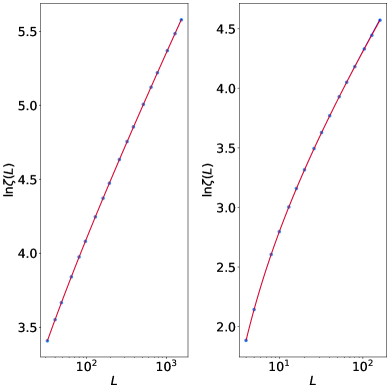
Figure 9: Average energy gap $\zeta=-\ln\overline{\Delta E}$ of the last decimated cluster versus the lattice size $L$ of the 2D (left) and 3D (right) $q=10$ Potts model. The curve is the non-linear fit $-\ln\overline{\Delta E}=a+bL^{\psi}$.

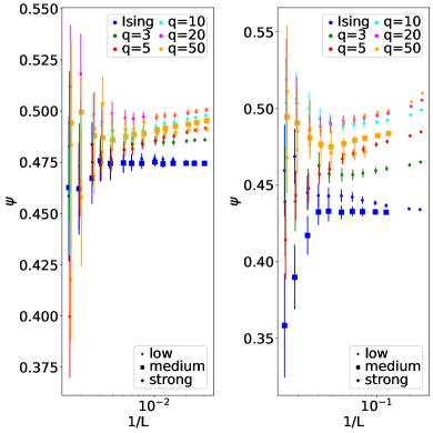
Figure 10: Effective exponent $\psi$ versus the smallest lattice size $L_{\rm min}$ entering into the fit for the 2D (left) and 3D (right) Potts models. The different colors correspond to different numbers of states $q$ of the Potts model. The different symbols correspond to different initial probability distributions of the couplings.

Table 2: Summary of the estimates of the critical exponents of the 2D and 3D random Potts models.

	$\nu_{s}$	$\nu_{w}$	$d_{f}$	$\psi$
2D	$1.25(6)$	$1.25(3)$	$1.021(5)$	$0.48(2)$
3D	$1.01(5)$	$0.985(10)$	$1.155(8)$	$0.46(4)$

VI Conclusions

When scaling corrections are not taken into account, the critical exponents $d_{f}$ and $\psi$ were shown to take, both in 2D and 3D, incompatible values that increase with the number of states $q$ of the Potts model. Since non-linear fits involving algebraic scaling corrections are unstable, effective exponents were estimated over shrinking ranges of lattice sizes $L\geq L_{\rm min}$. The limit $1/L_{\rm min}\rightarrow 0$ of these effective exponents is expected to give the critical exponent at the IDFP. The analysis is however hampered by the large fluctuations of the effective exponents, due to the smaller number of degrees of freedom in the fit at large $L_{\rm min}$. Nevertheless, scaling corrections are clearly observed. While the latter do not seem to depend on $q$ for the correlation length exponent (apart from $\nu_{s}$ in the 3D case), the corrections on the magnetic fractal dimension $d_{f}$ are strongly $q$-dependent. A shrinking of the dispersion of the effective exponents for different numbers of states $q$ is observed when $L_{\rm min}$ is increased, providing evidence of the existence of a super-universality class. This conclusion is in agreement with Ref. Vasseur where the super-universality of the 2D random Potts model is shown by means of a mapping onto a lattice gauge model. The effective exponents $\psi$ display a behavior similar to $d_{f}$, although less pronounced and with a residual dispersion of the exponents in the limit $1/L_{\rm min}\rightarrow 0$. Our final estimates of the critical exponents at the IDFP are summarized in Tab. 2. As noticed in the text, they are compatible with previous estimates obtained for the Ising model.

The question of the extension of the random quantum Ising universality class naturally arises. The 1D case was discussed in the introduction. In dimensions $d\geq 2$, it is not known whether the Ashkin-Teller model or the clock model also belong to the Ising universality class? There are some of the open questions that we will try to address in the future.

VII Bibliography

References

- (1) C. Dasgupta and S. Ma, Low-Temperature Properties of the Random Heisenberg Antiferromagnetic Chain, Phys. Rev. B 22, 1305 (1980).
- (2) D. S. Fisher, Random Transverse Field Ising Spin Chains, Phys. Rev. Lett. 69, 534 (1992).
- (3) D. S. Fisher, Critical Behavior of Random Transverse-Field Ising Spin Chains, Phys. Rev. B 51, 6411 (1995).
- (4) F. Iglói and C. Monthus, Strong Disorder RG Approach of Random Systems, Physics Reports 412, 277 (2005).
- (5) F. Iglói and C. Monthus, Strong disorder RG approach – a short review of recent developments, Eur. Phys. J. B 91, 290 (2018).
- (6) T. Vojta, J. Phys. A: Math. Gen. 39, R143 (2006).
- (7) F. Iglói, Exact Renormalization of the Random Transverse-Field Ising Spin Chain in the Strongly Ordered and Strongly Disordered Griffiths Phases, Phys. Rev. B 65, 064416 (2002).
- (8) T. Senthil and S. N. Majumdar, Critical Properties of Random Quantum Potts and Clock Models, Phys. Rev. Lett. 76, 3001 (1996).
- (9) J. Cardy and J. L. Jacobsen, Critical Behavior of Random-Bond Potts Models, Phys. Rev. Lett. 79, 4063 (1997).
- (10) C. Chatelain and B. Berche, Finite-Size Scaling Study of the Surface and Bulk Critical Behavior in the Random-Bond Eight-State Potts Model, Phys. Rev. Lett. 80, 1670 (1998).
- (11) J. L. Jacobsen and J. Cardy, Critical Behaviour of Random-Bond Potts Models: A Transfer Matrix Study, Nuclear Physics B 515, 701 (1998).
- (12) C. Chatelain and B. Berche, Universality and Multifractal Behaviour of Spin-Spin Correlation Functions in Disordered Potts Models, Nuclear Physics B 572, 626 (2000).
- (13) E. Carlon, P. Lajkó, and F. Iglói, Disorder Induced Cross-Over Effects at Quantum Critical Points, Phys. Rev. Lett. 87, 277201 (2001).
- (14) P. Goswami, D. Schwab, and S. Chakravarty, Phys. Rev. Lett. 100, 015703 (2008).
- (15) F. Hrahsheh, J. A. Hoyos, R. Narayanan, and T. Vojta, Strong-Randomness Infinite-Coupling Phase in a Random Quantum Spin Chain, Phys. Rev. B 89, 014401 (2014).
- (16) C. Chatelain and D. Voliotis, Numerical Evidence of the Double-Griffiths Phase of the Random Quantum Ashkin-Teller Chain, Eur. Phys. J. B 89, 18 (2016).
- (17) F. Hrahsheh, J. A. Hoyos, and T. Vojta, Rounding of a First-Order Quantum Phase Transition to a Strong-Coupling Critical Point, Phys. Rev. B 86, 214204 (2012).
- (18) H. Barghathi, F. Hrahsheh, J. A. Hoyos, R. Narayanan, and T. Vojta, Phys. Scr. T165, 014040 (2015).
- (19) A. K. Ibrahim and T. Vojta, Monte Carlo Simulations of the Disordered Three-Color Quantum Ashkin-Teller Chain, Phys. Rev. B 95, 054403 (2017).
- (20) C. Chatelain, Improved Matrix Product Operator Renormalization Group: Application to the N-Color Random Ashkin–Teller Chain, J. Stat. Mech. 2019, 093301 (2019).
- (21) O. Motrunich, S.-C. Mau, D. A. Huse, and D. S. Fisher, Infinite-Randomness Quantum Ising Critical Fixed Points, Phys. Rev. B 61, 1160 (2000).
- (22) I. A. Kovács and F. Iglói, Renormalization Group Study of the Two-Dimensional Random Transverse-Field Ising Model, Phys. Rev. B 82, 054437 (2010).
- (23) I. A. Kovács and F. Iglói, Infinite-Disorder Scaling of Random Quantum Magnets in Three and Higher Dimensions, Phys. Rev. B 83, 174207 (2011).
- (24) U. Agrawal, S. Gopalakrishnan, and R. Vasseur, Universality and Quantum Criticality in Quasiperiodic Spin Chains, Nature Communications 11, 1 (2020).
- (25) U. Agrawal, S. Gopalakrishnan, and R. Vasseur, Quantum Criticality in the 2d Quasiperiodic Potts Model, Phys. Rev. Lett. 125, 265702 (2020).
- (26) B. Kang, S.A. Parameswaran, A.C. Potter, R. Vasseur and S. Gazit, Superuniversality from disorder at two-dimensional topological phase transitions, Phys. Rev. B 102, 224204 (2020).
- (27) M. J. Stephen and L. Mittag, Pseudo-Hamiltonians for the Potts Model at the Critical Point, Physics Letters A 41, 357 (1972).
- (28) J. Sólyom and P. Pfeuty, Renormalization-Group Study of the Hamiltonian Version of the Potts Model, Phys. Rev. B 24, 218 (1981).
- (29) R. L. Greenblatt, M. Aizenman, and J. L. Lebowitz, Rounding of First Order Transitions in Low-Dimensional Quantum Systems with Quenched Disorder, Phys. Rev. Lett. 103, 197201 (2009).
- (30) M. Aizenman, R. L. Greenblatt, and J. L. Lebowitz, Proof of Rounding by Quenched Disorder of First Order Transitions in Low-Dimensional Quantum Systems, Journal of Mathematical Physics 53, 023301 (2012).
- (31) C. Chatelain, B. Berche, W. Janke, and P. E. Berche, Softening of First-Order Transition in Three-Dimensions by Quenched Disorder, Phys. Rev. E 64, 036120 (2001).
- (32) C. Chatelain, B. Berche, W. Janke, and P.-E. Berche, Monte Carlo Study of Phase Transitions in the Bond-Diluted 3D 4-State Potts Model, Nuclear Physics B 719, 275 (2005).
- (33) T.H. Cormen, C.E. Leiserson, R.L. Rivest, and C. Stein, Introduction to Algorithms, MIT Press and McGraw-Hill (2001)