Depth Evaluation for Metal Surface Defects by Eddy Current Testing using Deep Residual Convolutional Neural Networks

Abstract

Eddy current testing (ECT) is an effective technique in the evaluation of the depth of metal surface defects. However, in practice, the evaluation primarily relies on the experience of an operator and is often carried out by manual inspection. In this paper, we address the challenges of automatic depth evaluation of metal surface defects by virtual of state-of-the-art deep learning (DL) techniques. The main contributions are three-fold. Firstly, a highly-integrated portable ECT device is developed, which takes advantage of an advanced field programmable gate array (Zynq-7020 system on chip) and provides fast data acquisition and in-phase/quadrature demodulation. Secondly, a dataset, termed as MDDECT, is constructed using the ECT device by human operators and made openly available. It contains 48,000 scans from 18 defects of different depths and lift-offs. Thirdly, the depth evaluation problem is formulated as a time series classification problem, and various state-of-the-art 1-d residual convolutional neural networks are trained and evaluated on the MDDECT dataset. A 38-layer 1-d ResNeXt achieves an accuracy of 93.58% in discriminating the surface defects in a stainless steel sheet. The depths of the defects vary from 0.3 mm to 2.0 mm in a resolution of 0.1 mm. In addition, results show that the trained ResNeXt1D-38 model is immune to lift-off signals.

I Introduction

Eddy current testing (ECT) is a non-destructive testing (NDT) method harnessing the principle of electromagnetic induction, which, compared to other NDT methods, has the virtue of high speed, low cost and no contact [1]. These features make ECT an attractive technique in the detection and evaluation of surface defects for conductive materials [2]. Recovering the profiles of a defect, e.g. location and depth, from eddy current (EC) signals is a major topic in the research of ECT, where machine learning (ML) plays an important role [3].

Conventional ML algorithms have been adopted in various ECT applications, and many of these studies generally utilised a two-step approach. Firstly, raw EC signals would be subject to a feature transform or extraction process, such as Principle Component Analysis [4], time-frequency analysis by Rihaczek Distribution [5], Wavelet Transform [6], Hilbert–Huang Transform [7], geometry recognition from Lissajous Figure [8], and Convolutional Sparse Coding [9]. Next, the resultant feature representations, in order to achieve the ultimate task of detecting and classifying defects, would be fed to a classification or clustering algorithm such as Support Vector Machine (SVM) [6, 7, 8], Multi-Layer Perceptron [6], K-Means [4, 5], K-Nearest Neighbours [6, 8], Decision Tree [8] and Naive Bayes [8]. While these conventional ML algorithms still remain vibrant today in the research of ECT, Deep Learning (DL) methods prevail more recently, encouraged by their remarkable success in many other areas such as image classification.

A Deep Belief Network was exploited in [10] so as to, from the EC scan images of the defects on the surface of a Titanium sheet, extract features that were then fed to a least-square SVM algorithm to classify the defects. The dataset was also evaluated in [11] with a plain Convolutional Neural Network (CNN), which, in contrast to [10] where the feature extractor and classifier were separate, was trained end-to-end. In [12], an encoder-decoder CNN, named EddyNet, was proposed aiming at learning an inverse model, which predicted a crack profile given an EC signal. Training samples were procured from a forward model with inputs and outputs exchanged. In terms of pulsed ECT, a multi-task CNN was developed in [13], which installed a softmax layer and a fully connection layer as two outputs in order to simultaneously classify the type and predict the depth of flaw, respectively. In [14], a plain CNN was used to estimate the crack depth for a heat transfer tube of the steam generator of a pressurised water reactor, which, compared to conventional numerical models, was less computationally expensive at inference time. These DL-motivated studies all entailed a larger dataset compared to those using conventional ML algorithms. Specifically, the numbers of training samples in [13, 14, 12] were more than twenty thousand, while those in [5, 4, 7, 6, 9, 8] were mostly a few hundreds. In [11, 12, 13, 14], CNN was used which was one of the most popular networks in DL research. Nonetheless, the adopted CNNs were wide and shallow, which was at variance with the ‘deep’ feature of modern neural networks.

The recent advancement of CNN was largely driven by the ImageNet Large-Scale Visual Recognition Challenge (ILSVRC) [15]. AlexNet [16], the winner in 2012, was regarded as a break-through and drew attention on CNNs. In 2014, two very deep CNNs emerged. The first one was GoogLeNet (with Inception modules) [17], which adopted a sparsely connected architecture of stacking Inception modules composed of filters of various sizes. In contrast, the second, VGG [18], exploited smaller filters of the same size for all the convolutional layers and increased the depth. Both very deep CNNs were able to achieve compelling performances, however, they usually suffered the degradation problem [19] that training accuracy would saturate and then degrade as the depth increased. In 2015, ResNet [20] was proposed to address the degradation problem and won the ILSVRC-2015 with an ultra-deep network of 152 layers. The fundamental idea was to let the network fit a residual mapping, instead of the original propagation, by adding skipping connections between some layers, so that in principle a deep network would not produce higher training error than its shallower counterpart. The additional shortcut connections enabled gradients to propagate backwards to earlier layers more easily, and hence resulted in easier training than VGG. Later, ResNet evolved to the second version [21], where in each unit the activation layer preceded the convolutional layer. In 2016, ResNeXt [22] was proposed, which, in the residual module, harnessed the split-transform-merge pattern akin to the Inception module. These revolutionary CNN architectures have influenced many deep networks in applications beyond image classification. In particular, the state-of-the-art residual CNNs such as ResNet and ResNeXt can be applied to the research of defect depth estimation with ECT; however, it has not been seen in the literature.

In this paper, the problem of estimating the depth of a surface defect of a metallic sheet is addressed using a new ECT device and the state-of-the-art DL techniques. The main contributions are three-fold. Firstly, a portable multi-functional ECT device is introduced, which integrates an field programmable gate array (FPGA), an ARM processor and the Windows 10 operating system. Secondly, the defect depth estimation problem is formulated as a time series classification problem, and a dataset using the ECT device is constructed and made openly available. We name the dataset as MDDECT (Metal Defects of different Depths by ECT) and aim to initiate a data-sharing campaign. It can serve as a testbed and would encourage advancing the research of ECT in light of modern DL techniques. Lastly, the state-of-the-art residual CNNs are applied for the first time, to our knowledge, in the research of ECT. An accuracy rate of 93.58% is achieved using a 38-layer 1-d ResNeXt for defects with a depth resolution of 0.1 mm in a stainless steel sheet.

The remainder of the paper is organised as follows. LABEL:Sec:Residual-CNN-Architecture presents the architectures of the 1-d residual CNNs. The hardware design of the integrated ECT device is described in LABEL:Sec:Portable-ECT-Device. LABEL:Sec:ECT-Dataset introduces the procedures of data collection and the details of the MDDECT dataset. The configurations of hyper-parameters and training process are demonstrated, along with the results of different CNNs and discussions in LABEL:Sec:DCNN-Training-Experiment. The last section concludes the work and suggests further research directions.

II Architecture of 1-D Residual CNN

A residual CNN, e.g. ResNet, is constructed by stacking ‘residual units’, which learns a residual function $\mathcal{R}(x):=\mathcal{F}(x)-x$ where $\mathcal{F}(x)$ is the original underlying mapping [20]. Formally, a residual unit conducts calculations as expressed in (1), in which $x_{l}$ and $y_{l}$ are the input and output of the $l^{th}$ residual unit, respectively, and $\sigma$ is an activation function. The block $\mathcal{R}$ takes $x_{l}$ as input, and performs transformations with weights $W_{l}$. In the original version of ResNet, the activation function $\sigma$ is a rectified linear unit (ReLU). The block $\mathcal{R}$ is chosen from either a stack of two convolution units or a ‘bottleneck’ unit. A convolution unit is a convolution layer followed by a batch normalisation (BN) layer and a ReLU layer. A bottleneck unit comprises three convolution units, with the first and last convolution layers being 1$\times$1 convolutions, which are used to reduce dimensionality hence computational complexity.

In the second version of ResNet, the residual unit performs calculations as shown in (2), where the activation is an identity function [21]. However, the convolution unit in the block $\mathcal{R}$ is pre-activated, that is, the BN and ReLU layers precede the convolution layer. It was verified in [21] that (2) enabled gradients to propagate to any layers more easily than (1). In ResNeXt [22], the residual unit performs calculations as shown in (3), where the block $\mathcal{R}$ is an aggregation of a number of transformations $\mathcal{T}_{i}$, and the number $C$ is the cardinality. In practice, the split-transform-merge block $\mathcal{R}$ is usually implemented using an equivalent grouped convolution, where the number of groups equals the cardinality $C$. It is noted that here we assume that ResNeXt inherits from the second version of ResNet. In addition, the input $x_{l}$ and output $y_{l}$ share the same dimension in (1), (2) and (3) so as to illustrate the idea. When the dimensions are different, a convolution layer will replace the identity connection to match the dimensions.

$$y_{l}=\sigma\left(x_{l}+\mathcal{R}(x_{l},W_{l})\right)$$ (1)

$$y_{l}=x_{l}+\mathcal{R}(x_{l},W_{l})$$ (2)

$$y_{l}=x_{l}+\sum_{i=1}^{C}\mathcal{T}_{i}(x_{l},W_{li})$$ (3)

The convention of naming a network is followed in this paper by appending the version and depth to the type of network. However, because the convolution layers used are 1-d instead of 2-d, we append ‘1D’ to the name in order to differentiate the networks from the original 2-d ones. Usually, residual CNNs comprise multiple stages, each one of which has one or a stack of multiple residual units. In this paper, we unify the number of stages to four. The first residual unit of each stage doubles the channel dimension while halves the temporal dimension. In order to clarify details, LABEL:Fig:ResNet-Block-1 illustrates the architectures of ResNet1Dv1-14, ResNet1Dv2-14 and ResNeXt1D-14, which serve as the base-line networks for the defect depth classification task. They all have the same depth of 14 essential layers.

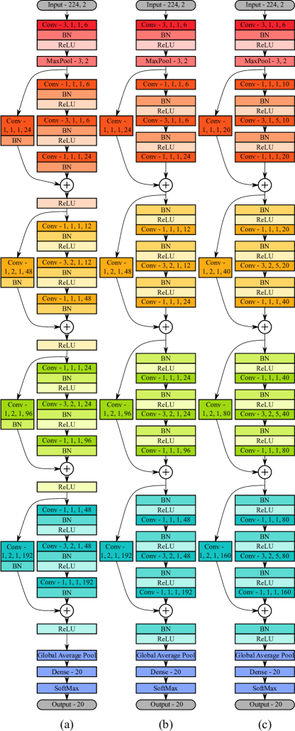
Figure 1: Detailed architectures of three 1-d residual networks. Four stages in each network are marked in different colours. The input tensor has 224 sampling points and 2 channels. In terms of the convolution layer, the numbers in the block represent the kernel size, strides, number of groups and number of filters. In terms of the max pooling layer, the numbers represent the kernel size and strides. The output tensor has 20 labels. (a), (b) and (c) correspond to ResNet1Dv1-14, ResNet1Dv2-14 and ResNeXt1D-14, respectively.

III Hardware Design of ECT Device

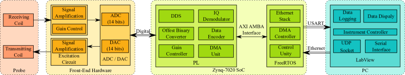
Figure 2: The block diagram of the architecture of the ECT device. The system is mainly composed of four modules, including a replaceable coil probe sensor, an SoC composed of an FPGA and an ARM processor, front-end circuits and a host PC running Windows 10 system.

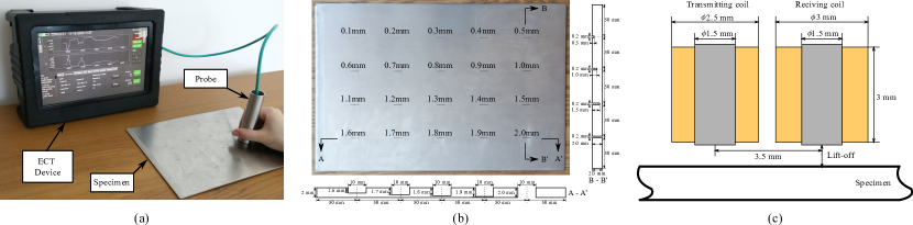
Figure 3: Images of the ECT device, specimen and probe sensor schematic. (a) illustrates a scene of a human operator scanning a steel sheet with a hand-hold probe sensor. (b) demonstrates the geometry dimensions of a steel sheet that is used as a specimen to collect data from. (c) shows the schematic of a probe sensor, which consists of two cylindrical ferrite-cored coils.

The architecture of the ECT device is shown in LABEL:Fig:Architecture-of-the. The system mainly consists of four components, which are a replaceable coil probe sensor, a Zynq-7020 system on chip (SoC), front-end circuits and a host PC. Zynq-7020 SoC is the cornerstone of the system, which integrates an ARM dual Cortex-A9 processor and a Xilinx 7-series FPGA. This module is responsible for generating excitation signals, implementing in-phase and quadrature (I/Q) demodulation and transferring data between the module and the host PC. The front-end circuits consist of ADC/DAC, signal amplification and gain control modules. A parallel digital interface is exploited to connect the front-end hardware and the SoC via an FPGA Mezzanine Card (FMC) connector. The system is capable of providing a multi-frequency excitation signal, and the received signal can be demodulated at each frequency simultaneously. The signal-to-noise ratio (SNR) of the output signal is above 80 dB on average. LABEL:Fig:Images-of-the(a) demonstrates a scene of a human operator holding a probe sensor and scanning a stainless steel sheet. The received signals and statistic information are displayed on the screen of the ECT device in real-time.

IV MDDECT Dataset

The success of deep learning in an application relies heavily on the effort of constructing large and well-labeled datasets. For instance, ImageNet contains 14 million high-quality images in 22 thousand visual categories [15]. However, it is difficult in principle to develop a universal dataset like ImageNet for defect depth estimation by ECT, because the impedance signal captured by an ECT sensor is determined by a plurality of factors. A widely accepted standard specimen with standard defects is lacking in the ECT research community.

The MDDECT dataset was constructed using the integrated ECT device described in LABEL:Sec:Portable-ECT-Device, which installed a probe sensor as shown in LABEL:Fig:Images-of-the(c). The excitation frequency was set as 20 kHz taking into account the system SNR and skin depth of the plate under test. The signal data rate was configured as 2,500 samples per second. A stainless steel sheet with 20 machine-fabricated slots on the surface was used as the specimen to scan, whose detailed geometry dimensions are shown in LABEL:Fig:Images-of-the(b). The defects were surface opening cracks, and shared the same length and width of 10 mm and 0.2 mm, respectively. The depth of the defects started from 0.1 mm and incremented by 0.1 mm to the largest 2.0 mm. The defect of 2.0 mm in depth was a through crack, as the thickness of the sheet was 2.0 mm.

Although the MDDECT dataset was specialised to the ECT device and the specimen, many other practical variances, which would nontrivially affect the performance of an ECT system, were taken into account. Firstly, thirty volunteers, who had no experience operating an ECT device, were invited to scan the defects, hence introducing a great variety of uncertainties, as composed to some research, e.g. [8, 9, 10, 11], where an automatically controlled movement was harnessed to scan defects. Secondly, lift-off signals were deliberately collected and labeled, so that the classifier should be able to differentiate lift-offs and defects. As seen in LABEL:Fig:Procedure(c), lift-off signals were generated by randomly tapping the probe to a defect-free area on the surface of the specimen. The lift-off distances were controlled to be under 3 mm above the surface. In addition, normal signals of defect-free areas were also captured and labeled, and the capturing process is illustrated in LABEL:Fig:Procedure(d). Thirdly, eight different scanning angles between the long-edge line of a defect and the line crossing the axial centres of the two coils were determined, as demonstrated in LABEL:Fig:[s]Procedure(a) and 4(b). Also, the volunteers scanned across a defect along an angle in two directions, back and forth. Lastly, when scanning a defect, the volunteers were asked to try to maintain a constant lift-off distance of 0.5 mm, constant moving speed of 60 mm/s and hold the probe vertical to the surface. However, variances were inevitable and represented more practical testing scenarios, hence making the MDDECT challenging.

After a preliminary test, it was found that the signals of the defects of 0.1 mm and 0.2 mm were under the noise floor, and hence the data from these two defects were excluded from the dataset. As a result, the total number of classes was 20, including 18 classes of defects, the lift-off class and normal signal class. Each volunteer repeated the same scanning 5 times. All scans were divided into scan segments, each of time window 0.5 seconds, which gave rise to the temporal dimension of 1250. Ultimately, the dataset tensor had dimensions of (30, 8, 2, 5, 20, 1250, 2), each one of which represented the number of volunteers, scanning angles, directions, repeats of each scanning, classes, temporal points, and channels, respectively. The last dimension corresponded to the in-phase and quadrature channels. In total, the MDDECT comprehended 48,000 scan segments (or scans for simplicity) in 20 classes. In terms of the split of training and test sets, volunteers and the data scanned by them were randomly selected. As a result, the dimensions for training and test sets are (43200, 1250, 2) and (4800, 1250, 2), respectively, constituting 90% and 10% of the total samples. Hence the test set consists of three randomly selected volunteers. The MDDECT dataset is available on Kaggle.

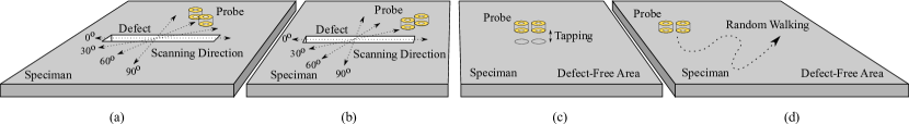
Figure 4: Illustrations of data collecting processes. (a) and (b) demonstrate the probe scanning across a defect in eight different angles and two directions (back and forth). Notice that the line crossing the axial centres of the two coils is either tangental or normal to the scanning direction. (c) shows the probe tapping on the surface of a defect-free area in order to generate lift-off signals. (d) shows the probe moving in a random trajectory on the surface of a defect-free area in order to generate normal signals.

V Experiment Details and Results

Before training a network, we needed to extract and set aside a validation set from the training set, in order to determine hyper-parameters and select DL models. The test set must not be used in the training phase, and should only serve to produce the final claim on accuracy. As the training set contains data from 27 volunteers, we randomly selected 3 from the 27 volunteers and used their corresponding data as a validation set. In addition, the temporal dimension was decimated from 1250 to 250 by a factor of 5, in order to enable a faster training. As a result, the dimensions of the training, validation and test sets were (38400, 250, 2), (4800, 250, 2) and (4800, 250, 2), respectively. The ratio of the number of samples among them was 8:1:1.

V-A Normalise and augment data

The final training data was applied with a channel-wise normalisation according to (4), where $x_{i}$ is the flattened tensor when the channel dimension equals $i$, and $\mu_{i}$ and $\sigma_{i}$ are the mean and standard deviation of $x_{i}$, respectively. This normalisation is termed as z-normalisation [23], which nullifies the mean and standardises the variance of the data in terms of each channel. The resultant training data was then used to train a network. In addition, the calculated $\mu_{i}$ and $\sigma_{i}$ from the training data were used to normalise the validation and test data too. In order to appreciate the data in general before training, the z-normalised validation data are plotted all together in a complex plane in LABEL:Fig:Signal-Comparison, from which it can be seen that the lift-off signals are larger in magnitude and also different in phase compared to the defect signals. However, most signals overlap severely with each other, indicating the difficulties to classify these signals.

$$\frac{x_{i}-\mu_{i}}{\sigma_{i}},i=1,2$$ (4)

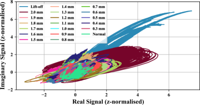
Figure 5: The z-normalised validation data all together in a complex plane. The mean and standard deviation used in the normalisation were calculated from the training data. The x and y axes represent the in-phase and quadrature channels, respectively.

After normalisation, the data was then configured for train-time and test-time augmentations. In terms of train-time augmentation, every training sample was cropped randomly for every epoch in order to introduce certain variances to the training data on the fly. Concretely, a segment of dimensions (224, 2) was cropped randomly under a uniform distribution from the original training sample of dimensions (250, 2). As a result, the input dimensions to a network were (224, 2), where the batch dimension was not shown. In terms of test-time augmentation, 10-crop test was conducted to the validation and test samples, that is, the final classification result of a sample was determined by averaging the outputs of a network for 10 random crops from the sample.

TABLE I: Architecture Details of Residual CNNs

Stage	Output Size	Network Architecture
		ResNet1Dv1-26	ResNet1Dv2-26	ResNeXt1D-26	ResNet1Dv1-14	ResNet1Dv2-14	ResNeXt1D-14 (Wider 1)	ResNeXt1D-14 (Wider 2)	ResNeXt1D-38
					(Wider)	(Wider)
	224	conv - 3, 1, 1, 6	conv - 3, 1, 1, 6	conv - 3, 1, 1, 6	conv - 3, 1, 1, 8	conv - 3, 1, 1, 8	conv - 3, 1, 1, 8	conv - 3, 1, 1, 8	conv - 3, 1, 1, 6
	112	max pool - 3, 2
1	112	$\left[\begin{array}[]{c}1,6\\ 3,6\\ 1,24\end{array}\right]\times 2$	$\left[\begin{array}[]{c}1,6\\ 3,6\\ 1,24\end{array}\right]\times 2$	$\left[\begin{array}[]{c}1,10\\ 3,10,C=5\\ 1,20\end{array}\right]\times 2$	$\left[\begin{array}[]{c}1,8\\ 3,8\\ 1,32\end{array}\right]\times 1$	$\left[\begin{array}[]{c}1,8\\ 3,8\\ 1,32\end{array}\right]\times 1$	$\left[\begin{array}[]{c}1,14\\ 3,14,C=7\\ 1,28\end{array}\right]\times 1$	$\left[\begin{array}[]{c}1,15\\ 3,15,C=5\\ 1,30\end{array}\right]\times 1$	$\left[\begin{array}[]{c}1,10\\ 3,10,C=5\\ 1,20\end{array}\right]\times 3$
2	56	$\left[\begin{array}[]{c}1,12\\ 3,12\\ 1,48\end{array}\right]\times 2$	$\left[\begin{array}[]{c}1,12\\ 3,12\\ 1,48\end{array}\right]\times 2$	$\left[\begin{array}[]{c}1,20\\ 3,20,C=5\\ 1,40\end{array}\right]\times 2$	$\left[\begin{array}[]{c}1,16\\ 3,16\\ 1,64\end{array}\right]\times 1$	$\left[\begin{array}[]{c}1,16\\ 3,16\\ 1,64\end{array}\right]\times 1$	$\left[\begin{array}[]{c}1,28\\ 3,28,C=7\\ 1,56\end{array}\right]\times 1$	$\left[\begin{array}[]{c}1,30\\ 3,30,C=5\\ 1,60\end{array}\right]\times 1$	$\left[\begin{array}[]{c}1,20\\ 3,20,C=5\\ 1,40\end{array}\right]\times 3$
3	28	$\left[\begin{array}[]{c}1,24\\ 3,24\\ 1,96\end{array}\right]\times 2$	$\left[\begin{array}[]{c}1,24\\ 3,24\\ 1,96\end{array}\right]\times 2$	$\left[\begin{array}[]{c}1,40\\ 3,40,C=5\\ 1,80\end{array}\right]\times 2$	$\left[\begin{array}[]{c}1,32\\ 3,32\\ 1,128\end{array}\right]\times 1$	$\left[\begin{array}[]{c}1,32\\ 3,32\\ 1,128\end{array}\right]\times 1$	$\left[\begin{array}[]{c}1,80\\ 3,80,C=7\\ 1,160\end{array}\right]\times 1$	$\left[\begin{array}[]{c}1,60\\ 3,60,C=5\\ 1,120\end{array}\right]\times 1$	$\left[\begin{array}[]{c}1,40\\ 3,40,C=5\\ 1,80\end{array}\right]\times 3$
4	14	$\left[\begin{array}[]{c}1,48\\ 3,48\\ 1,192\end{array}\right]\times 2$	$\left[\begin{array}[]{c}1,48\\ 3,48\\ 1,192\end{array}\right]\times 2$	$\left[\begin{array}[]{c}1,80\\ 3,80,C=5\\ 1,160\end{array}\right]\times 2$	$\left[\begin{array}[]{c}1,64\\ 3,64\\ 1,256\end{array}\right]\times 1$	$\left[\begin{array}[]{c}1,64\\ 3,64\\ 1,256\end{array}\right]\times 1$	$\left[\begin{array}[]{c}1,160\\ 3,160,C=7\\ 1,320\end{array}\right]\times 1$	$\left[\begin{array}[]{c}1,120\\ 3,120,C=5\\ 1,240\end{array}\right]\times 1$	$\left[\begin{array}[]{c}1,80\\ 3,80,C=5\\ 1,160\end{array}\right]\times 3$
	1	global average pool, 20-d fc, softmax
# Trainable Parameters		$9.37\times 10^{4}$	$9.30\times 10^{4}$	$9.38\times 10^{4}$	$1.01\times 10^{5}$	$1.00\times 10^{5}$	$9.77\times 10^{4}$	$1.14\times 10^{5}$	$1.35\times 10^{6}$
FLOPs		$3.70\times 10^{6}$	$3.69\times 10^{6}$	$3.84\times 10^{6}$	$4.11\times 10^{6}$	$4.09\times 10^{6}$	$4.25\times 10^{6}$	$4.99\times 10^{6}$	$5.42\times 10^{6}$

V-B Determine network architectures and hyper-parameters

As discussed in LABEL:Sec:Residual-CNN-Architecture, the networks exploited in this paper were one-dimensional variants of the residual CNNs. In addition, the CNNs were fixed to have four stages, and hence the minimal depth was 14 for each network, where only one residual module existed in each stage. LABEL:Fig:ResNet-Block-1 illustrates the architectures of ResNet1Dv1-14, ResNet1Dv2-14 and ResNeXt1D-14, which served as the base-line networks. The width of them, that is, the number of filters in the first convolution layer, was set to 6. They all had a similar level of trainable parameters and floating point operations (FLOPs).

Based upon the three base-line networks, we experimented on the depth dimension and doubled the number of residual modules in each stage of the networks, which gave rise to three deeper networks: ResNet1Dv1-26, ResNet1Dv2-26 and ResNeXt1D-26. In addition, we also attempted to expand the width dimension from the base-line networks while maintaining the number of trainable parameters and FLOPs similar to the 26-layer ones, which gave rise to four wider networks. The details of the architectures of these seven new networks are listed in LABEL:Tab:deeperandwider. As they had a similar computation complexity, we would be able to compare their performances and see whether depth or width was more effective under the scope of this paper. Lastly, we evaluated our deepest network ResNeXt1D-38, where in each stage there were three residual modules. The details of the architecture of ResNeXt1D-38 are listed in the last column in LABEL:Tab:deeperandwider.

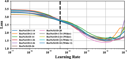
Figure 6: Losses v.s. learning rate. The best initial learning rate appears to be the same for all the evaluated networks, which is about 4.0$\times$10^-5 and marked by a dotted vertical line in the figure.

Learning rate is an important hyper-parameter affecting the training and performance of a network. In order to find the best initial learning rate, we performed the strategy from [24], where the training started with a small learning rate and increased it epoch by epoch in a geometric progression. After a few epochs, the loss v.s. learning rate plot could be drawn, and the best initial learning rate located at the point where the loss decreased most rapidly. This strategy was applied to all the networks we evaluated, and the resultant plots of loss v.s. learning rate are shown in LABEL:Fig:Data-Augmentation-2. It can be seen that all the networks appear to share the same best learning rate 4.0$\times$10^-5, at which the losses descend rapidly. It is noted that this way of finding the best initial learning rate may not an exact solution. Notice that the x-axis in the figure is in a logarithmic scale.

All the networks were applied with the same following training configurations and hyper-parameters. Adam optimiser was exploited with default values of parameters recommended in [25], and the mini-batch size was set to 128. The training data were shuffled for every epoch, and each network was trained for 10,000 epochs. The learning rate was initialised to 4.0$\times$10^-5, and decreased to 4.0$\times$10^-6 at epoch 5,000, and finally to 4.0$\times$10^-7 at epoch 7,500.

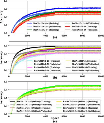
Figure 7: Training processes of eleven networks. (a), (b) and (c) depict the training and validation accuracies for three base-line networks, four deeper networks and four wider networks, respectively. Solid and dashed lines represent the training and validation accuracies, respectively. Results of the same network use similar colours.

V-C Train networks and analyse results

The training was coded using the Tensorflow library, and conducted on an Nvidia RTX 2080Ti GPU. In total, the training of the networks took about five days to finish. The training and validation accuracies and losses are displayed in LABEL:Fig:Training-on-MD for three base-line networks: ResNet1Dv1-14, ResNet1Dv2-14 and ResNeXt1D-14, four deeper networks: ResNet1Dv1-26, ResNet1Dv2-26, ResNeXt1D-26 and ResNeXt1D-38, and four wider ResNet1Dv1-14, ResNet1Dv2-14 and ResNeXt1D-14 with respect to training epoch, which are also available as a TensorBoard experiment.

Three main observations can be taken from the training processes. Firstly, the three base-line networks all suffer the under-fitting problem as per LABEL:Fig:Training-on-MD(a), that is, they converge to large training errors between 15% and 10%, which implies that their representation powers are insufficient for the MDDECT dataset. Such suggestion is verified by the results of larger networks in LABEL:Fig:Training-on-MD(b) and 7(c), where the training errors of ResNet1Dv1-26, ResNet1Dv2-26 and ResNeXt1D-26 are well below 5%, and the training errors of the wider ResNet1Dv1-14, ResNet1Dv2-14 and ResNeXt1D-14 are slightly higher than 5%. On the other hand, the validation errors of the larger networks are around 10%. However, it’s difficult to conclude that the larger networks are over-fitted to the training data, only based on the about 5% difference between the training and validation errors. Secondly, the deeper networks in general have achieved higher accuracies than the wider ones that share similar level of trainable parameters and FLOPs, as can be seen by comparing LABEL:Fig:Training-on-MD(b) and 7(c). Thirdly, different versions and types of network lead to marginal differences in terms of both the training and validation accuracies. In LABEL:Fig:Training-on-MD(b), the discrepancies of the training and validation accuracies of ResNet1Dv1-26, ResNet1Dv2-26 and ResNeXt1D-26 are within 3%. The discrepancies in LABEL:Fig:Training-on-MD(c) are even smaller. However, ResNeXt1D-26 has achieved the best performance among the larger networks of similar levels of complexity. As a consequence, we further trained a ResNeXt1D-38, the deepest network we evaluated, so as to test the limit of performance. Its training and validation accuracies are plotted in LABEL:Fig:Training-on-MD(b).

TABLE II: Classification Results

Network Architecture	Accuracy
	Top-1	± 0.1mm
ResNet1Dv1-14	87.88%	95.14%
ResNet1Dv2-14	83.21%	93.01%
ResNeXt1D-14	86.65%	94.51%
ResNet1Dv1-26	92.50%	96.90%
ResNet1Dv2-26	91.85%	96.06%
ResNeXt1D-26	93.15%	96.78%
ResNet1Dv1-14 (Wider)	90.42%	95.88%
ResNet1Dv2-14 (Wider)	89.93%	95.65%
ResNeXt1D-14 (Wider 1)	91.31%	96.23%
ResNeXt1D-14 (Wider 2)	89.38%	95.00%
ResNeXt1D-38	93.58%	97.20%

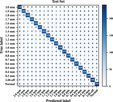
Figure 8: Confusion matrix of the trained ResNeXt1D-38 on the test set. Every entry in the matrix represents the number of samples that are classified to a specific class.

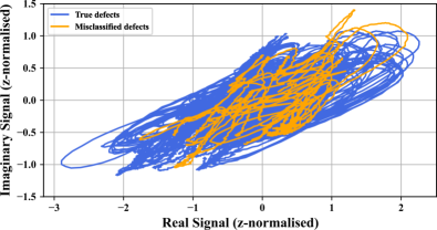
Figure 9: The z-normalised signals in the complex plane for the samples in the test set that are predicted as the 1.4 mm defect from the trained ResNeXt1D-38 model. Blue and yellow traces represent the true and misclassified samples, respectively.

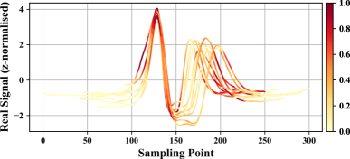
Figure 10: The real signals of the samples of the 2.0 mm defects in the test set with class activation mappings calculated based on the trained ResNeXt1D-38. The colour represents the activation level of a sampling point with respect to the 2.0 mm defect class. The plots are aligned according to their first peaks in order to clarify the activation regions.

In order to claim the final accuracies, the best trained model of a network was selected as the one that achieved the highest validation accuracy during training for that network. Next, the test set data was fed to the chosen model to produce the final claimed accuracy of the network. The final top-1 accuracies of each network are listed in LABEL:Tab:Results. It can be seen that ResNeXt1D-38 has achieved the highest accuracy of 93.58%, while the second best accuracy is 93.15%, achieved by ResNeXt1D-26. The fact that the additional 12 layers give rise to an improvement of only 0.43% implies that simply increasing the depth may not be able to push the boundary of performance, and over-fitting may occur. Moreover, if the accuracy metric is relaxed to tolerate an error of $\pm$ 0.1 mm, the ‘$\pm$ 0.1 mm accuracies’ are also listed in the same table, where ResNeXt1D-38 also wins with 97.20%. If we examine closer on the results of ResNeXt1D-38, its confusion matrices on the test set is shown in LABEL:Fig:Confusion-Matrix-2-1. It can be seen that the mistaken samples tend to be classified into the adjacent classes of their ground-truth classes, which explains the much improved 97.20% accuracy with $\pm$ 0.1 mm tolerances. In addition, it appears that shallower defects are not more difficult to classify than deeper ones. Lastly, the lift-off samples are all correctly detected. Being immune to lift-off signals is an important and desirable feature for an ECT defect depth estimation method.

In order to further understand the misclassified samples, we can plot the data according to their predicted labels. For instance, the test set data labeled as the 1.4 mm defect by the trained ResNeXt1D-38 are plotted in LABEL:Fig:Plots-of-the, from which it can be seen that, the wrongly labeled samples overlap in great deal with the correct samples. This phenomenon can be found for other defects as well. We argue that it is almost impossible to estimate by human the depth of a defect in the resolution of 0.1 mm, while ResNeXt1D-38 has achieved a 93.58% accuracy. A Class Activation Mapping (CAM) can be calculated as per [26] to examine the contributions of every sampling points to the classification of a time series. As an illustration, CAMs for the samples of the 2.0 mm defect in the test set were calculated based on the trained ResNeXt1D-38, and are shown in LABEL:Fig:Class-Activation-Mapping. It can be seen that only some regions of the time series are activated and other regions are masked out. This can help explain why ResNeXt1D-38 is able to correctly differentiate samples of different classes that have overlapping parts, because they have different activation regions for their own classes. Moreover, it is worth pointing out that the times series of the same class share similar activation regions, as can be clearly seen in LABEL:Fig:Class-Activation-Mapping.

VI Conclusions

The evaluation of the depth of a surface defect of metallic materials is a major application of ECT, where, recent DL-motivated methods commence to surpass the conventional ones. However, many existing approaches have not taken full advantage of the state-of-the-art DL techniques proposed in computer vision. In this paper, we aim at addressing the problem of ECT-based surface defect depth estimation by using 1-d deep residual convolutional networks. Firstly, a highly integrated and multi-functional portable ECT device is developed based on Zynq-7020 SoC, which provides fast data acquisition and I/Q demodulation. Secondly, a dataset, termed as the MDDECT, is constructed by 30 volunteer operators using the ECT device, and consists of 48,000 samples of 20 classes in total. The MDDECT dataset is openly available and can be exploited as a testbed in order to promote new ECT algorithms. Thirdly, eleven 1-d residual networks of three different types are evaluated, and a 38-layer network network ResNeXt1D-38 has achieved an accuracy of 93.58% in terms of estimating the depth of the surface defects from 0.3 mm to 2.0 mm with depth resolution of 0.1 mm. In addition, the deep learning algorithms can reject lift-off signal, hence immune to lift-off noise. Future research directions would be to evaluate a different family of deep networks such as recurrent networks and other learning strategies. Moreover, a continued effort should be made to enrich the MDDECT dataset with more diversities, scans and specimens.

References

- [1] A. Sophian, G. Y. Tian, D. Taylor, and J. Rudlin, “Electromagnetic and eddy current NDT: a review,” Insight, vol. 43, no. 5, p. 6, 2001.
- [2] J. García-Martín, J. Gómez-Gil, and E. Vázquez-Sánchez, “Non-Destructive Techniques Based on Eddy Current Testing,” Sensors, vol. 11, no. 3, pp. 2525–2565, Feb. 2011.
- [3] K. Bin Ali, A. N. Abdalla, D. Rifai, and M. A. Faraj, “Review on system development in eddy current testing and technique for defect classification and characterization,” Iet Circuits Devices & Systems, vol. 11, no. 4, pp. 338–351, Jul. 2017.
- [4] J. Kim, G. Yang, L. Udpa, and S. Udpa, “Classification of pulsed eddy current GMR data on aircraft structures,” NDT & E International, vol. 43, no. 2, pp. 141–144, Mar. 2010.
- [5] S. Hosseini and A. A. Lakis, “Application of time–frequency analysis for automatic hidden corrosion detection in a multilayer aluminum structure using pulsed eddy current,” NDT & E International, vol. 47, pp. 70–79, Apr. 2012.
- [6] R. Smid, A. Docekal, and M. Kreidl, “Automated classification of eddy current signatures during manual inspection,” NDT & E International, vol. 38, no. 6, pp. 462–470, Sep. 2005.
- [7] B. Liu and Z. Li, “Study on the automatic recognition of hidden defects based on Hilbert Huang transform and hybrid SVM-PSO model,” in 2017 Prognostics and System Health Management Conference (PHM-Harbin), pp. 1–7, Jul. 2017.
- [8] L. Yin, B. Ye, Z. Zhang, Y. Tao, H. Xu, J. R. Salas Avila, and W. Yin, “A novel feature extraction method of eddy current testing for defect detection based on machine learning,” NDT & E International, vol. 107, p. 102108, Oct. 2019.
- [9] Y. Tao, H. Xu, J. R. S. Avila, C. Ktistis, W. Yin, and A. J. Peyton, “Defect Feature Extraction in Eddy Current Testing Based on Convolutional Sparse Coding,” in 2019 IEEE International Instrumentation and Measurement Technology Conference (I2MTC), pp. 1–6, May. 2019.
- [10] J. Bao, B. Ye, X. Wang, and J. Wu, “A Deep Belief network and Least Squares Support Vector Machine Method for Quantitative Evaluation of Defects in Titanium Sheet Using Eddy Current Scan Image,” Frontiers in Materials, vol. 7, p. 576806, Sep. 2020.
- [11] W. Deng, J. Bao, and B. Ye, “Defect Image Recognition and Classification for Eddy Current Testing of Titanium Plate Based on Convolutional Neural Network,” Complexity, Oct. 2020.
- [12] S. Li, A. Anees, Y. Zhong, Z. Yang, Y. Liu, R. S. M. Goh, and E.-X. Liu, “Learning to Reconstruct Crack Profiles for Eddy Current Nondestructive Testing,” in Workshop on Machine Learning and the Physical Sciences, Vancouver, Canada, Dec. 2019.
- [13] X. Fu, C. Zhang, X. Peng, L. Jian, and Z. Liu, “Towards end-to-end pulsed eddy current classification and regression with CNN,” in 2019 IEEE International Instrumentation and Measurement Technology Conference (I2MTC), pp. 1–5, May. 2019.
- [14] K. Demachi, T. Hori, and S. Perrin, “Crack depth estimation of non-magnetic material by convolutional neural network analysis of eddy current testing signal,” Journal of Nuclear Science and Technology, vol. 57, no. 4, pp. 401–407, Apr. 2020.
- [15] J. Deng, W. Dong, R. Socher, L. Li, Kai Li, and Li Fei-Fei, “ImageNet: A large-scale hierarchical image database,” in 2009 IEEE Conference on Computer Vision and Pattern Recognition, pp. 248–255, Jun. 2009.
- [16] A. Krizhevsky, I. Sutskever, and G. E. Hinton, “ImageNet Classification with Deep Convolutional Neural Networks,” in Advances in Neural Information Processing Systems 25, F. Pereira, C. J. C. Burges, L. Bottou, and K. Q. Weinberger, Eds., pp. 1097–1105. Curran Associates, Inc., 2012.
- [17] C. Szegedy, Wei Liu, Yangqing Jia, P. Sermanet, S. Reed, D. Anguelov, D. Erhan, V. Vanhoucke, and A. Rabinovich, “Going deeper with convolutions,” in 2015 IEEE Conference on Computer Vision and Pattern Recognition (CVPR), pp. 1–9, Jun. 2015.
- [18] K. Simonyan and A. Zisserman, “Very Deep Convolutional Networks for Large-Scale Image Recognition,” in 3rd International Conference on Learning Representations (ICLR), San Diego, CA, USA, May. 2015.
- [19] R. Srivastava, K. Greff, and J. Schmidhuber, “Highway Networks,” ArXiv, 2015.
- [20] K. He, X. Zhang, S. Ren, and J. Sun, “Deep Residual Learning for Image Recognition,” in 2016 IEEE Conference on Computer Vision and Pattern Recognition (CVPR), pp. 770–778, Jun. 2016.
- [21] K. He, X. Zhang, S. Ren, and J. Sun, “Identity Mappings in Deep Residual Networks,” in Computer Vision – ECCV 2016, ser. Lecture Notes in Computer Science, B. Leibe, J. Matas, N. Sebe, and M. Welling, Eds., pp. 630–645. Cham: Springer International Publishing, 2016.
- [22] S. Xie, R. Girshick, P. Dollár, Z. Tu, and K. He, “Aggregated Residual Transformations for Deep Neural Networks,” in 2017 IEEE Conference on Computer Vision and Pattern Recognition (CVPR), pp. 5987–5995, Jul. 2017.
- [23] H. Ismail Fawaz, G. Forestier, J. Weber, L. Idoumghar, and P.-A. Muller, “Deep learning for time series classification: a review,” Data Mining and Knowledge Discovery, Mar. 2019.
- [24] L. N. Smith, “Cyclical Learning Rates for Training Neural Networks,” in 2017 IEEE Winter Conference on Applications of Computer Vision (WACV), pp. 464–472, Mar. 2017.
- [25] D. P. Kingma and J. Ba, “Adam: A Method for Stochastic Optimization,” CoRR, vol. abs/1412.6980, 2015.
- [26] B. Zhou, A. Khosla, A. Lapedriza, A. Oliva, and A. Torralba, “Learning Deep Features for Discriminative Localization,” in 2016 IEEE Conference on Computer Vision and Pattern Recognition (CVPR), pp. 2921–2929, Jun. 2016.