Kubo Formula for Non-Hermitian Systems and Tachyon Optical Conductivity

Abstract

Linear response theory plays a prominent role in various fields of physics and provides us with extensive information about the thermodynamics and dynamics of quantum and classical systems. Here we develop a general theory for the linear response in non-Hermitian systems with nonunitary dynamics and derive a modified Kubo formula for the generalized susceptibility for an arbitrary (Hermitian and non-Hermitian) system and perturbation. We use this to evaluate the dynamical response of a non-Hermitian, one-dimensional Dirac model with imaginary and real masses, perturbed by a time-dependent electric field. The model has a rich phase diagram, and in particular, features a tachyon phase, where excitations travel faster than an effective speed of light. Surprisingly, we find that the dc conductivity of tachyons is finite, and the optical sum rule is exactly satisfied for all masses. Our results highlight the peculiar properties of the Kubo formula for non-Hermitian systems and are applicable for a large variety of settings.

Introduction.

Linear response theory is a fundamental framework in many branches of physics that describes the way in which a physical system responds to small external perturbations and allows us to interpret physical measurements [1]. The response is expressed in terms of a generalized susceptibility of the unperturbed system. The change in the expectation value of an operator $A$ due to a time-dependent perturbation $V(t)=Bf(t)$ is assumed to be linear in the perturbative force $f(t)$,

$$\delta\langle A(t)\rangle=\int dt^{\prime}\chi_{AB}(t,t^{\prime})f(t^{\prime})\,,$$ (1)

with $\chi_{AB}(t,t^{\prime})$ known as the response function. In general, $\chi_{AB}(t,t^{\prime})$ is real, and for systems invariant under time translations $\chi_{AB}(t,t^{\prime})=\chi_{AB}(t-t^{\prime})$. Traditionally, the explicit expression for the response function in Eq. (1) is given by the Kubo formula [2], and has been for decades a standard tool in the study of electric transport and spin susceptibilities in response to applied electric and magnetic fields in typical many-body [3, 4, 5], closed [6, 7], or open systems [8, 9, 10]. Through the fluctuation-dissipation theorem, the linear response provides information about the equilibrium fluctuations of a system, and can reveal, e.g., topological properties through the quantum Hall response [11] or demonstrate the presence of fractional charge carriers for the fractional quantum Hall effect via noise measurements [12].

Recently, a newly emerging field of non-Hermitian physics [13, 14, 15, 16, 17, 18, 19] has become very active, mostly for its promising applications [17] and for exhibiting unique features, which are absent in the Hermitian realm, such as exceptional points [20, 21, 22, 23, 24], non-Hermitian skin effect [25, 26, 27, 28, 29], non-Bloch phase transitions [30], and unidirectional invisibility [31], to mention a few. By now, quantum optics and cold atoms setups provide fertile grounds where such non-Hermitian concepts are probed experimentally [21, 32, 33, 34]. In such state-of-the-art experiments, e.g., in a quantum gas microscopy experiment [35, 36], the measurement backaction can qualitatively alter the low-energy physics, so it is crucial to understand and describe the effect of small perturbations in such non-Hermitian systems. In this regard, only recently, a non-Hermitian perturbation of a Hermitian Hamiltonian has been considered, and a modified Kubo formula for the generalized susceptibility has emerged [37]. Still, at present, a complete non-Hermitian linear response theory, in which the Hamiltonian governing the system and the perturbation are both non-Hermitian, is missing.

In the present work we address this problem, and fill this gap, by developing a general formalism and providing a generalized Kubo formula for the susceptibility $\chi_{AB}(t,t^{\prime})$ introduced in Eq. (1) which is suitable for non-Hermitian systems under very general conditions. We use our approach by computing the correlation function for the current operator, in response to an external electric field, and the associated optical conductivity for a non-Hermitian tachyon model. Although non-Hermiticity is in general associated with dissipation, we find remarkable features such as a finite dc conductivity in the absence of scatterers or local charge conservation, which guarantees that the optical sum rule is satisfied [38].

General theory.

We consider a general setup in which the system is modeled by a time-independent non-Hermitian Hamiltonian $H_{0}$ with a nondegenerate spectrum subjected to a time-dependent perturbation $V(t)=Bf(t)$, which starts to act at $t=0$, where $B$ is an operator which can be non-Hermitian and $f(t)$, the perturbation force, is assumed to be small and real-valued. We are interested in the linear response of a system operator $\delta\langle A(t)\rangle=\langle A(t)\rangle-\langle A\rangle_{0}$. The expectation value $\langle A(t)\rangle$ at time $t$ is given by [39]

$$\langle A(t)\rangle=\frac{\text{tr}[\rho(t)A]}{\text{tr}[\rho(t)]},$$ (2)

where $\rho(t)$ is the density matrix of the system in the Schrödinger representation obeying the non-Hermitian von Neumann equation $i\hbar\partial_{t}\rho(t)=H\rho(t)-\rho(t)H^{\dagger}$, with $H=H_{0}+V(t)$, the full Hamiltonian. Its solution is decomposed as $\rho(t)=\rho_{0}(t)+\delta\rho(t)$ with $\rho_{0}(t)=e^{-iH_{0}t/\hbar}\rho(0)e^{iH_{0}^{\dagger}t/\hbar}$, the density matrix of the unperturbed system, and $\delta\rho(t)$ arising from the external perturbation. Rotating to the interaction picture (see Supplemental Material for more details), the variation $\delta\langle A(t)\rangle$ is evaluated to first order in the perturbation as

$$\delta\langle A(t)\rangle=\frac{\textrm{tr}[\delta\rho_{I}(t)A_{I}(t)]}{\textrm{tr}[\rho_{0}(t)]}-\langle A(t)\rangle_{0}\frac{\textrm{tr}[\delta\rho(t)]}{\textrm{tr}[\rho_{0}(t)]},$$ (3)

where $A_{I}(t)=e^{iH_{0}^{\dagger}t/\hbar}Ae^{-iH_{0}t/\hbar}$ is written in the interaction representation in terms of the unperturbed system, and $\delta\rho_{I}(t)=e^{iH_{0}t/\hbar}\delta\rho(t)e^{-iH_{0}^{\dagger}t/\hbar}$. The second, norm correction term, is specific to nonunitary dynamics and is absent in the unitary evolution, yet it is important to reproduce correctly the dynamics of the expectation values. The expectation value dynamics of an operator $A$ acquires additional terms, due to the fact that $H\neq H^{\dagger}$ and the wave function norm is not conserved. Keeping in mind that $A_{I}(t)$ is identical to the Heisenberg picture time evolution in terms of $H_{0}$, i.e., $A(t)=A_{I}(t)$, we finally obtain a compact expression for the generalized susceptibility defined in Eq. (1) as

$$\chi_{AB}(t,t^{\prime})=-\frac{i}{\hbar}\theta(\tau)\textrm{tr}\bigg{\{}\bigg{[}[A(\tau),B]_{\sim}-\langle A(t)\rangle_{0}[e^{iH_{0}^{\dagger}\tau/\hbar}e^{-iH_{0}\tau/\hbar},B]_{\sim}\bigg{]}\cdot\frac{\rho_{0}(t^{\prime})}{\textrm{tr}[\rho_{0}(t)]}\bigg{\}},$$ (4)

in terms of a modified commutator defined as $[X,Y]_{\sim}=XY-Y^{\dagger}X$, where $\tau=t-t^{\prime}$. The first term is the natural generalization of the Hermitian Kubo formula for the non-Hermitian setting. The second term arises solely from the nonunitary dynamics, and $\langle A(t)\rangle_{0}={\text{tr}[\rho_{0}(t)A]}/{\text{tr}[\rho_{0}(t)]}$. In contrast to the Hermitian Kubo formula, the non-Hermitian counterpart is not time-translation invariant and depends separately on $t$ and $t^{\prime}$ due to the appearance of the system density matrix $\rho_{0}(t)$ at various times, which may have a nonunitary evolution in the absence of the perturbation. Finally, note that expectation values are obtained using the right eigenvectors of the system Hamiltonian, which is a conventional approach to treat non-Hermitian systems as effective models of dissipative dynamics with no quantum jumps [40, 41]. An alternative route, would be to use a biorthogonal basis [42]. This approach is usually employed for a class of non-Hermitian Hamiltonians invariant under space-time reflection ($\mathcal{PT}$) symmetry, and endowed with a real spectrum in the $\mathcal{PT}$-symmetric phase  [43, 13]. Various $\mathcal{PT}$-symmetric Hamiltonians have been extensively studied especially in photonics by controlling gain and loss [21, 44, 45, 46, 32]. The eigenspectrum reality is a property shared by a larger class of pseudo-Hermitian Hamiltonians [47, 48], and allows us to map a non-Hermitian $\mathcal{PT}$-symmetric Hamiltonian, onto a Hermitian Hamiltonian with unitary evolution, by using a positive definite pseudometric operator. However, the biorthogonal approach is unsuitable for the broken $\mathcal{PT}$-symmetry phase, where the Hamiltonian possesses complex pairs of eigenvalues and such a mapping does not exist [47, 49, 50].

When the system Hamiltonian $H_{0}$ is Hermitian, the expression (4) simplifies considerably since $\rho_{0}(t)=\rho(0)$ is a time-independent equilibrium density matrix. For example, if additionally, the perturbation proves Hermitian, the norm corrections drop out, and assuming that the system is invariant under time translation, one readily recovers the regular Kubo formula [1], $\chi(\tau)=-\frac{i}{\hbar}\theta(\tau)\langle[A(\tau),B]\rangle_{0}$. If the perturbation is anti-Hermitian $B^{\dagger}=-B$, the correlation function recovers the central result of Ref. [37], where the modified commutator becomes an anticommutator, $\chi(\tau)=-\frac{i}{\hbar}\theta(\tau)(\langle\{A(\tau),B\}\rangle_{0}-2\langle A\rangle_{0}\langle B\rangle_{0})$. Finally, for a $\mathcal{PT}$-symmetric model, in the symmetric phase, or for any pseudo-Hermitian model with a real eigenspectrum, where the initial density matrix is constructed from the ground-state wave function, the correlation function Eq. (4) simplifies to

$$\chi_{AB}(\tau) = -\frac{i}{\hbar}\theta(\tau)\langle[A(\tau),B]_{\sim}-$$ (5)

$$-\langle A(0)\rangle_{0}[e^{iH_{0}^{\dagger}\tau/\hbar}e^{-iH_{0}\tau/\hbar},B]_{\sim}\rangle_{0}.$$

If $H_{0}$ is non-Hermitian, the norm correction term is crucial and it cannot be discarded as it may encompass the dominant contribution to linear response.

Non-Hermitian Dirac Hamiltonian.

Using our results in Eq. (4), we investigate a rather generic one-dimensional (1D) non-Hermitian Dirac model which contains a tachyon phase [51]. Such a non-Hermitian Hamiltonian has been recently realized experimentally on waveguide lattices on a photonic chip [52, 53] as well as proposed as an effective Hamiltonian in an ion trap experiment [54]. The system Hamiltonian in momentum space is

$$H_{0}=\sum_{p}p\,c\,\sigma_{x}+\Delta\sigma_{y}-imc^{2}\sigma_{z},$$ (6)

which has two momentum-dependent energy bands $E_{\pm}(p)=\pm\varepsilon(p)$, with $\varepsilon(p)=\sqrt{p^{2}c^{2}+\Delta^{2}-m^{2}c^{4}}$ [see Fig. 1(a)], with the Fermi velocity as the effective light speed $c$. The Hamiltonian is invariant with respect to a $\mathcal{PT}$-symmetry operator $\sigma_{x}\mathcal{K}$, with $\mathcal{K}$ performing complex conjugation, $[\sigma_{x}\mathcal{K},H_{0}]=0$. The gapped non-Hermitian Dirac Hamiltonian at $|\Delta|>mc^{2}$ is in a $\mathcal{PT}$-symmetric phase since the eigenvectors are invariant to the $\mathcal{PT}$-symmetry operator and the spectrum consists of two real energy bands [43, 13, 47]. In this regime, the density of states, $g(\omega)=\sum_{p}\delta(\omega-E_{\pm}(p))$ vanishes below the gap edge and features a sharp threshold singularity at $\sqrt{\Delta^{2}-m^{2}c^{4}}$. Exactly at $|\Delta|=mc^{2}$, the spectrum becomes gapless with a linear dispersion $\varepsilon(p)=c|p|$. The $p=0$ point marks an exceptional point (EP), where not only the eigenvalues, but also the eigenvectors coalesce [20, 22]. Because of the linear dispersion, the density of states is constant for all energies. For $|\Delta|<mc^{2}$, a tachyonlike spectrum with a hyperbolic gapless dispersion develops. Depending on $p$, the system is in a $\mathcal{PT}$-symmetric phase with real eigenvalues for $p^{2}c^{2}>m^{2}c^{4}-\Delta^{2}$ or in a $\mathcal{PT}$-symmetry broken phase, with conjugate pairs of imaginary eigenvalues, at $p^{2}c^{2}<m^{2}c^{4}-\Delta^{2}$. These two momentum regions are separated by EPs at $\varepsilon(p_{\rm EP})=0$. Close to the EP, the spectrum behaves as $|\varepsilon(p)|\sim\sqrt{p-p_{\rm EP}}$, and consequently $g(\omega)\sim\omega$ for small energies. This is reminiscent of the case of 2D graphene [55], but in 1D such a behavior is only possible for non-Hermitian systems. Close to the EP, the group velocity diverges as $\partial_{p}\varepsilon(p)\sim 1/\sqrt{p-p_{\rm EP}}$.

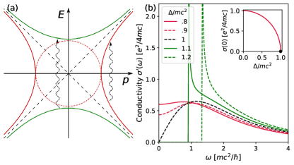
Figure 1: (a) Dispersion relation for the non-Hermitian Hamiltonian (6) with (green) parabolic spectrum of gapped Dirac Hamiltonians at $|\Delta|>mc^{2}$, (red) hyperbolic tachyon dispersion for $|\Delta|<mc^{2}$, and (black) linear Dirac spectrum at $|\Delta|=mc^{2}$. The dispersion is imaginary (dashed-dotted line) only in the tachyon phase for $p^{2}c^{2}<m^{2}c^{4}-\Delta^{2}$. The wiggly lines denote resonant optical transitions under the applied electric field. (b) The real part of the conductivity $\sigma^{\prime}(\omega)$ as a function of frequency for several values of the ratio $\Delta/mc^{2}$ in the case of (green) parabolic, (black) linear, or (red) hyperbolic (tachyon) dispersion. (Inset) Tachyon dc conductivity as a function of $\Delta/mc^{2}$.

As a perturbation, we consider a time-dependent electric field $\mathcal{E}$ that couples to the current operator and induces optical transitions between the two bands. The electric field effect is taken into account through a time-dependent vector potential $\mathcal{A}(t)$ as $p\to p+e\mathcal{A}(t)$, with $e$, the absolute value of electric charge, and $\mathcal{E}=-\partial\mathcal{A}/\partial t$. Then the perturbation couples to the vector potential through the current operator $j=-\delta H/\delta\mathcal{A}=\sum_{p}j_{p}$, with $j_{p}=-ec\sigma_{x}$. In spite of being non-Hermitian, $H_{0}$ is still gauge invariant [56, 38] . This also implies that the local charge density $\langle n(x)\rangle$ is conserved and the continuity equation holds [58]

$$-e\partial_{t}\langle n(x)\rangle+\partial_{x}\langle j(x)\rangle=0,$$ (7)

which guarantees that the optical sum rule is satisfied, as we discuss later.

Optical conductivity.

Our main task is to determine the current-current correlator $\chi(t,t^{\prime})\equiv-\chi_{jj}(t,t^{\prime})$ using Eq. (4) and the corresponding optical conductivity, that describes the optical response to the external electric field. As initial conditions we assume the half filling case. In the gapped and $\mathcal{PT}$-symmetric tachyon phases, the system starts in the ground state with all the $-\varepsilon(p)$ levels initially occupied, while in the $\mathcal{PT}$-symmetry broken phase the levels with a larger weight, and corresponding to the slowest decay rate, associated with $+i|\varepsilon(p)|$ states dominate the dynamics at $t<0$ [58] are assumed to be filled.

First of all, we find that while in general the perturbation causes transitions between the bands, the response is zero in the broken $\mathcal{PT}$-symmetry phase for tachyons, i.e., when the spectrum consists of pairs of imaginary eigenvalues. This is due to exact cancellation between the generalized commutator contribution to the response, $[j_{p}(\tau),j_{p}(0)]$, and the norm corrections. We have also checked this numerically by solving Eq. (6) in the presence of a weak electromagnetic field. Therefore, only the $\mathcal{PT}$-symmetric part of the model with pairs of real eigenvalues contributes to linear response. The initial conditions fix $\rho_{0}(t)=\rho(0)$, and Eq. (5) becomes

$$\chi(\tau) = {\sum_{p}}^{\prime}\frac{\chi(p,\tau)}{L}=\frac{i\theta(\tau)}{\hbar\,L}{\sum_{p}}^{\prime}\langle[j_{p}(\tau),j_{p}(0)]\rangle_{0}$$ (8)

$$-\langle j_{p}(0)\rangle_{0}\langle[e^{iH_{0}^{\dagger}\tau/\hbar}e^{-iH_{0}\tau/\hbar},j_{p}(0)]\rangle_{0},$$

where $L$ is the system size and $\sum_{p}^{\prime}$ restricts the sum to momenta in the $\mathcal{PT}$-symmetric region $p^{2}c^{2}>m^{2}c^{4}-\Delta^{2}$. For our particular model, at half filling, $\chi(\tau)$ is time-translation invariant, unlike the general formula in Eq. (4).

First we consider the case $\Delta=0$ with purely imaginary mass, where the salient features of non-Hermitian linear response are clearly manifested. Noticing that the Hamiltonian $H_{0}(\Delta=0)$ is self-conjugate with respect to $\sigma_{x}$, it implies $[j_{p},H_{0}(\Delta=0)]_{\sim}=0$, and therefore the current operator is time independent. Hence the first contribution to $\chi(\tau)$ in Eq. (8), containing the commutator $[j_{p}(\tau),j_{p}(0)]=0$, drops out. However, the norm correction term remains finite and contributes to the linear response. Such a term is unique to non-Hermitian systems, without any analogue in the conventional Hermitian Kubo formula.

For generic real gap $\Delta$, both the generalized commutator and the norm correction terms contribute, and $\chi(p,\tau)$ reads

$$\chi(p,\tau)=\frac{2e^{2}c^{2}}{\hbar}\theta(\tau)\frac{(\varepsilon(p)\Delta-pmc^{3})^{2}}{(p^{2}c^{2}+\Delta^{2})^{2}}\sin\frac{2\varepsilon(p)\tau}{\hbar}.$$ (9)

The result recovers correctly the Hermitian limit $m\to 0$ [59, 60]. The correlation function (9) captures an interesting behavior for the Dirac-point dispersion $|\Delta|=mc^{2}$: only half of the momenta contribute to linear response. Indeed, for $p>0$ and $\Delta=mc^{2}$, $\chi(p>0,\tau)=0$ and $\langle j_{p>0}(t)\rangle=ec$, while for $p<0$ and $\Delta=-mc^{2}$, $\chi(p<0,\tau)=0$ and $\langle j_{p<0}(t)\rangle=-ec$. This is a result of destructive quantum interference, due to the two masses of equal amplitude, that inhibits half of the momentum states to transition from the ground to the excited states [58]. This is analogous to unidirectional invisibility in non-Hermitian systems [31, 17]. Our construction is based on the assumption of a non-degenerate spectrum, so exactly at the EP the theory does not apply. Nevertheless, for any choice of parameters that brings the system close to the EP, the linear theory remains valid [58], and in particular, the correlation function vanishes close to the EP on both sides, which indicates that one would not expect unphysical anomalies due to the EP.

The time dependent $\chi(\tau)$ is obtained by summation over all momentum states. We find that in the gapped phase $\chi(\tau)$ exhibits a damped oscillating behavior with a slow decay $\sim\tau^{-1/2}$ which transforms into an exponential decay for the linear dispersion and in the tachyon phase [58]. The response in frequency space $\chi(\omega)$ follows by Fourier transforming Eq. (9) and summing over momenta. The real (absorptive) part of the optical conductivity is given by the imaginary part of the susceptibility, $\sigma^{\prime}(\omega)=\chi^{\prime\prime}(\omega)/\omega$ [58].

Figure 1(b) displays the evolution of $\sigma^{\prime}(\omega)$ in all three regimes. For $|\Delta|=mc^{2}$, the dispersion is linear, similarly to the gapless 1D Dirac equation, but, in contrast to the expectations from a 1D Hamiltonian $\sim pc\sigma_{x}$, where $\sigma^{\prime}(\omega)=0$ [60], now $\sigma^{\prime}(\omega>0)>0$. This is a manifestation of Zitterbewegung, and follows from the noncommutativity of the current operator and Hamiltonian, due to the additional real and imaginary mass terms [61, 62].

The conductivity in the gapped phase $|\Delta|>mc^{2}$, behaves qualitatively similar to the one in the gapped Hermitian model [60]. There is a threshold for excitations given by the band gap $\hbar\omega\simeq 2\,\sqrt{\Delta^{2}-m^{2}c^{4}}$, above which a threshold singularity appears, similarly to the density of states.

Finally, in the tachyon phase $|\Delta|<mc^{2}$, $\sigma^{\prime}(\omega)$ remains always finite, with no anomalous behavior when the system approaches the EP, although the group velocity $\partial_{p}\varepsilon(p)$ diverges at the EPs. The low-frequency constant optical conductivity parallels closely to graphene, where the linear density of states produces similar behavior. Furthering this analogy with graphene, we also identify a nonzero dc conductivity $\sigma_{\rm dc}=\sigma(\omega=0)$ for tachyons which depends on the ratio of the effective gap and the imaginary mass,

$$\sigma_{\rm dc}=\frac{e^{2}}{4mc}\frac{|\sqrt{\Delta^{2}-m^{2}c^{4}}|}{mc^{2}},$$ (10)

while $\sigma_{\rm dc}=0$ for $|\Delta|\geq mc^{2}$. A finite dc conductivity without scatterers was only thought to be possible for graphene [63, 55] in 2D, and the present 1D non-Hermitian Dirac system represents another occurrence. However, with increasing frequency, the analogy with graphene stops, as the EPs do not play a major role and the optical conductivity decays with frequency as $\sim\omega^{-3}$. Finally, as a consequence of the local charge conservation [58, 38], the optical sum rule [1] is satisfied for all phases of the non-Hermitian model,

$$\int_{0}^{\infty}\sigma^{\prime}(\omega)d\omega=\frac{e^{2}c}{2\hbar}.$$ (11)

It would be interesting to investigate this and other sum rules in non-Hermitian, higher dimensional systems as well.

Connection to experiments.

Our general theory is expected to find applications in a variety of non-Hermitian settings [18], where additional external perturbations reveal various aspects of the underlying model. For example, the role of topology in non-Hermitian systems, combined with many-body physics, as well as various sources of dissipation can be probed using our theory.

In terms of the tachyon physics, imaginary mass particle dynamics has been recently demonstrated experimentally in waveguide lattices [52], and in single-photon interferometric devices [53], thus realizing the effective non-Hermitian Hamiltonian (6). The waveguide lattices are composed by alternating waveguides where either loss or gain is dominant, and an alternating coupling coefficient between the propagating modes. The mode propagation in the paraxial approximation is then mapped to a Dirac-like Hamiltonian where the imaginary mass results from the interplay between the ratio of coupling coefficients and gain/loss rates. Experiments on single-photon interferometry [53] have already realized Eq. (6). Because of the extreme tunability of this setup, additional perturbations such as a frequency dependent vector potential can be engineered, and the current can be measured separately for each $p$ mode. From this, $\chi(p,\tau)$ is determined, whose knowledge yields the optical conductivity.

Another promising avenue involves ion trap physics, which allows us to simulate the 1D Dirac equation in a minimal setup consisting of two atomic levels and a motional degree of freedom [64, 65, 54]. In such setups, the density matrix of the system evolves according to a Lindblad equation [66, 67], but postselecting outcomes with no photon emission events singles out the dynamics driven by the non-Hermitian Hamiltonian in Eq. (6). Finally, the optical conductivity can be measured by in situ fluorescence spectroscopy [68].

Conclusions.

To sum up, we developed a unified linear response theory for non-Hermitian systems and perturbations, and provided an expression for the Kubo formula suitable for non-Hermitian models. It contains (i) a generalized commutator, (ii) norm correction terms due to nonunitary dynamics, and (iii) is not generally time-translation invariant. Through the generalized commutator, the non-Hermitian linear response gives direct experimental access to unequal-time anticommutators of observables instead of commutators, quantities hard to measure within the Hermitian realm.

We applied it to investigate the optical conductivity of a generic one-dimensional Dirac model, with both real and imaginary masses. This model features a tachyon phase where excitations travel faster than an effective speed of light. We find that the low-energy physics in this phase is graphenelike with constant optical conductivity and finite minimal conductivity. For all masses, the optical sum rule is satisfied. We argue that these results can be tested experimentally. Our Kubo formula represents an ideal starting point to gain information about non-Hermitian many-body systems as well, where the available methods are limited.

References

- Mahan [2000] G. D. Mahan, Many-Particle Physics, 3rd ed. (Kluwer, Boston, 2000).
- Kubo [1957] R. Kubo, J. Phys. Soc. Jpn. 12, 570 (1957).
- Baranger and Stone [1989] H. U. Baranger and A. D. Stone, Phys. Rev. B 40, 8169 (1989).
- Crépieux and Bruno [2001] A. Crépieux and P. Bruno, Phys. Rev. B 64, 014416 (2001).
- Nagaosa et al. [2010] N. Nagaosa, J. Sinova, S. Onoda, A. H. MacDonald, and N. P. Ong, Rev. Mod. Phys. 82, 1539 (2010).
- Cohen [2003] D. Cohen, Phys. Rev. B 68, 155303 (2003).
- Bohr et al. [2006] D. Bohr, P. Schmitteckert, and P. Wölfle, Europhys. Lett. 73, 246 (2006).
- Michel et al. [2004] M. Michel, J. Gemmer, and G. Mahler, Eur. Phys. J. B 42, 555 (2004).
- Fujii [2007] T. Fujii, J. Phys. Soc. Jpn. 76, 044709 (2007).
- Kundu et al. [2009] A. Kundu, A. Dhar, and O. Narayan, J. Stat. Mech.: Theory Exp. 2009 (03), L03001.
- Thouless et al. [1982] D. J. Thouless, M. Kohmoto, M. P. Nightingale, and M. den Nijs, Phys. Rev. Lett. 49, 405 (1982).
- Saminadayar et al. [1997] L. Saminadayar, D. C. Glattli, Y. Jin, and B. Etienne, Phys. Rev. Lett. 79, 2526 (1997).
- Bender [2007] C. M. Bender, Rep. Prog. Phys. 70, 947 (2007).
- Rotter [2009] I. Rotter, J. Phys. A: Math. Theor. 42, 153001 (2009).
- Moiseyev [2011] N. Moiseyev, Non-Hermitian Quantum Mechanics (Cambridge University Press, Cambridge New York, 2011).
- Cao and Wiersig [2015] H. Cao and J. Wiersig, Rev. Mod. Phys. 87, 61 (2015).
- El-Ganainy et al. [2018] R. El-Ganainy, K. G. Makris, M. Khajavikhan, Z. H. Musslimani, S. Rotter, and D. N. Christodoulides, Nat. Phys. 14, 11 (2018).
- Ashida et al. [2020] Y. Ashida, Z. Gong, and M. Ueda, Adv. Phys. 69, 249 (2020).
- Bergholtz et al. [2021] E. J. Bergholtz, J. C. Budich, and F. K. Kunst, Rev. Mod. Phys. 93, 015005 (2021).
- Berry [2004] M. V. Berry, Czech. J. Phys. 54, 1039 (2004).
- Makris et al. [2008] K. G. Makris, R. El-Ganainy, D. N. Christodoulides, and Z. H. Musslimani, Phys. Rev. Lett. 100, 103904 (2008).
- Heiss [2012] W. D. Heiss, J. Phys. A: Math. Theor. 45, 444016 (2012).
- Zhen et al. [2015] B. Zhen, C. W. Hsu, Y. Igarashi, L. Lu, I. Kaminer, A. Pick, S.-L. Chua, J. D. Joannopoulos, and M. Soljačić, Nature 525, 354 (2015).
- Dóra et al. [2019] B. Dóra, M. Heyl, and R. Moessner, Nat. Commun. 10, 2254 (2019).
- Yao and Wang [2018] S. Yao and Z. Wang, Phys. Rev. Lett. 121, 086803 (2018).
- Kunst et al. [2018] F. K. Kunst, E. Edvardsson, J. C. Budich, and E. J. Bergholtz, Phys. Rev. Lett. 121, 026808 (2018).
- Song et al. [2019] F. Song, S. Yao, and Z. Wang, Phys. Rev. Lett. 123, 246801 (2019).
- Li et al. [2020a] L. Li, C. H. Lee, and J. Gong, Phys. Rev. Lett. 124, 250402 (2020a).
- Borgnia et al. [2020] D. S. Borgnia, A. J. Kruchkov, and R.-J. Slager, Phys. Rev. Lett. 124, 056802 (2020).
- Longhi [2019] S. Longhi, Phys. Rev. Research 1, 023013 (2019).
- Lin et al. [2011] Z. Lin, H. Ramezani, T. Eichelkraut, T. Kottos, H. Cao, and D. N. Christodoulides, Phys. Rev. Lett. 106, 213901 (2011).
- El-Ganainy et al. [2019] R. El-Ganainy, M. Khajavikhan, D. N. Christodoulides, and S. K. Özdemir, Commun. Phys. 2, 37 (2019).
- Li et al. [2020b] L. Li, C. H. Lee, S. Mu, and J. Gong, Nat. Commun. 11, 5491 (2020b).
- Takasu et al. [2020] Y. Takasu, T. Yagami, Y. Ashida, R. Hamazaki, Y. Kuno, and Y. Takahashi, Prog. Theor. Exp. Phys. 2020, 12A110 (2020).
- Bakr et al. [2009] W. S. Bakr, J. I. Gillen, A. Peng, S. Fölling, and M. Greiner, Nature 462, 74 (2009).
- Kuhr [2016] S. Kuhr, Natl. Sci. Rev. 3, 170 (2016).
- Pan et al. [2020] L. Pan, X. Chen, Y. Chen, and H. Zhai, Nat. Phys. 16, 767 (2020).
- Benfatto et al. [2005] L. Benfatto, S. G. Sharapov, N. Andrenacci, and H. Beck, Phys. Rev. B 71, 104511 (2005).
- Graefe et al. [2008] E. M. Graefe, H. J. Korsch, and A. E. Niederle, Phys. Rev. Lett. 101, 150408 (2008).
- Daley [2014] A. J. Daley, Adv. Phys. 63, 77 (2014).
- Herviou et al. [2019] L. Herviou, N. Regnault, and J. H. Bardarson, SciPost Phys. 7, 69 (2019).
- Brody [2014] D. C. Brody, J. Phys. A: Math. Theor. 47, 035305 (2014).
- Bender and Boettcher [1998] C. M. Bender and S. Boettcher, Phys. Rev. Lett. 80, 5243 (1998).
- Musslimani et al. [2008] Z. H. Musslimani, K. G. Makris, R. El-Ganainy, and D. N. Christodoulides, Phys. Rev. Lett. 100, 030402 (2008).
- Guo et al. [2009] A. Guo, G. J. Salamo, D. Duchesne, R. Morandotti, M. Volatier-Ravat, V. Aimez, G. A. Siviloglou, and D. N. Christodoulides, Phys. Rev. Lett. 103, 093902 (2009).
- Özdemir et al. [2019] Ş. K. Özdemir, S. Rotter, F. Nori, and L. Yang, Nat. Mater. 18, 783 (2019).
- Mostafazadeh [2002] A. Mostafazadeh, J. Math. Phys. 43, 205 (2002).
- Zhang and You [2019] G.-Q. Zhang and J. Q. You, Phys. Rev. B 99, 054404 (2019).
- Mostafazadeh [2007] A. Mostafazadeh, Phys. Lett. B 650, 208 (2007).
- Gardas et al. [2016] B. Gardas, S. Deffner, and A. Saxena, Sci. Rep. 6, 23408 (2016).
- Feinberg [1967] G. Feinberg, Phys. Rev. 159, 1089 (1967).
- Song et al. [2020] W. Song, S. Gao, H. Li, C. Chen, S. Wu, S. Zhu, and T. Li, arXiv e-prints (2020), 2011.08496 [physics.optics] .
- Xiao et al. [2021] L. Xiao, D. Qu, K. Wang, H.-W. Li, J.-Y. Dai, B. Dóra, M. Heyl, R. Moessner, W. Yi, and P. Xue, PRX Quantum 2, 020313 (2021).
- Lee et al. [2015] T. E. Lee, U. Alvarez-Rodriguez, X.-H. Cheng, L. Lamata, and E. Solano, Phys. Rev. A 92, 032129 (2015).
- Castro Neto et al. [2009] A. H. Castro Neto, F. Guinea, N. M. R. Peres, K. S. Novoselov, and A. K. Geim, Rev. Mod. Phys. 81, 109 (2009).
- Merzbacher [1998] E. Merzbacher, Quantum Mechanics (Wiley, New York, 1998).
- Note [1] Gauge invariance in our case means that a time dependent electric field can equally be represented by a vector or a scalar potential.
- [58] D. Sticlet, B. Dora, and C. P. Moca, Supplementary Material .
- Dóra and Simon [2015] B. Dóra and F. Simon, Sci. Rep. 5, 14844 (2015).
- Lee et al. [1974] P. Lee, T. Rice, and P. Anderson, Solid State Commun. 14, 703 (1974).
- Cserti and Dávid [2006] J. Cserti and G. Dávid, Phys. Rev. B 74, 172305 (2006).
- Thaller [2011] B. Thaller, The Dirac Equation (Springer, 2011).
- Katsnelson [2006] M. I. Katsnelson, Eur. Phys. J. B 51, 157 (2006).
- Lamata et al. [2007] L. Lamata, J. León, T. Schätz, and E. Solano, Phys. Rev. Lett. 98, 253005 (2007).
- Gerritsma et al. [2010] R. Gerritsma, G. Kirchmair, F. Zähringer, E. Solano, R. Blatt, and C. F. Roos, Nature 463, 68 (2010).
- Lindblad [1976] G. Lindblad, Comm. Math. Phys. 48, 119 (1976).
- Gorini et al. [1976] V. Gorini, A. Kossakowski, and E. C. G. Sudarshan, J. Math. Phys. 17, 821 (1976).
- Anderson et al. [2019] R. Anderson, F. Wang, P. Xu, V. Venu, S. Trotzky, F. Chevy, and J. H. Thywissen, Phys. Rev. Lett. 122, 153602 (2019).