Large factor model estimation
by nuclear norm plus $l_{1}$ norm penalization

Abstract

This paper provides a comprehensive estimation framework via nuclear norm plus $l_{1}$ norm penalization for high-dimensional approximate factor models with a sparse residual covariance. The underlying assumptions allow for non-pervasive latent eigenvalues and a prominent residual covariance pattern. In that context, existing approaches based on principal components may lead to misestimate the latent rank, due to the numerical instability of sample eigenvalues. On the contrary, the proposed optimization problem retrieves the latent covariance structure and exactly recovers the latent rank and the residual sparsity pattern. Conditioning on them, the asymptotic rates of the subsequent ordinary least squares estimates of loadings and factor scores are provided, the recovered latent eigenvalues are shown to be maximally concentrated and the estimates of factor scores via Bartlett’s and Thompson’s methods are proved to be the most precise given the data. The validity of outlined results is highlighted in an exhaustive simulation study and in a real financial data example.

1 Introduction

The digital revolution has enormously enlarged the amount of available data for researchers and practitioners. Consequently, the need rises to develop methodologies able to summarize the content of high-dimensional datasets, in order to derive meaningful information from them.

The factor model is an effective tool to this end, as it detects the latent covariance structure behind a set of variables. We can define the factor model for any $p$-dimensional mean-centered random vector $x$ as

$$x=Bf+\epsilon,$$ (1)

where $B$ is a $p\times r$ matrix, $f$ is a $r\times 1$ random vector with $E(f)=0_{r}$ and $V(f)=I_{r}$, and $\epsilon$ is a $p\times 1$ random vector with $E(\epsilon)=0_{p}$ and $V(\epsilon)=S^{*}$, with $S^{*}$ full rank $p\times p$ matrix.

Let us indicate by $\Sigma^{*}$ the $p\times p$ covariance matrix of the random vector $x$. Assuming that $f$ and $\epsilon$ are componentwise uncorrelated, the factor model (1) induces in $\Sigma^{*}$ a low rank plus residual decomposition of the following type:

$$\Sigma^{*}=L^{*}+S^{*}=BB^{\prime}+S^{*},$$ (2)

where $L^{*}=BB^{\prime}=U_{L}\Lambda_{L}U_{L}^{\prime}$, with $U_{L}$ $p\times r$ semi-orthogonal matrix and $\Lambda_{L}$ $r\times r$ diagonal matrix. The representation (2) is invariant under orthogonal transforms, and it is therefore unidentifiable from the data without further constraints.

Suppose that we have a sample $x_{k}$, $k=1,\ldots,n$. The unbiased $p\times p$ sample covariance matrix is defined as $\Sigma_{n}=(n-1)^{-1}{\sum_{k=1}^{n}x_{k}x_{k}^{\prime}}$. Most of factor model estimation methods rely on $\Sigma_{n}$ as an input, and make essentially use of two techniques: principal component analysis (see Jolliffe (2002) for an overview) and maximum likelihood. As outlined in (Bai et al., 2008), however, a large dimension $p$ leads to some particular estimation problems for model (1), due to the limitations of $\Sigma_{n}$ in high dimensions.

From a historical perspective, the classical inferential theory for factor models (Anderson, 1958) prescribes that the dimension $p$ is fixed while the sample size $n$ tends to infinity. In particular, the strict condition $p<n$ is required to ensure consistency. As a consequence, the classical framework is clearly inappropriate if $p$ is large. When $p>n$, in fact, $\Sigma_{n}$ becomes inconsistent and no longer Wishart-distributed.

At the same time, when the dimension $p$ and the sample size $n$ are finite, Anderson and Rubin (1956) show that the use of the principal components of $\Sigma_{n}$ to estimate $B$ leads to loadings and factor scores estimates which are incoherent with model assumptions, because any estimate of $S^{*}$ so derived will never be full rank. That is the reason why Chamberlain and Rothschild (1983) prove that the principal components of $\Sigma_{n}$ consistently identify $L^{*}$ under model (1) as $p\rightarrow\infty$, provided that the $r$ eigenvalues of $L^{*}$ diverge with $p$ and $S^{*}$ is a non-diagonal matrix with vanishing eigenvalues as $p$ diverges.

Another relevant aspect concerns the ratio $p/n$. If $p/n\rightarrow 1^{-}$, the bad conditioning properties of $\Sigma_{n}$ inevitably affect the consistency of principal component analysis (PCA) as a factor model estimation method. In fact, the sample eigenvalues follow the Marcenko-Pastur law (Marčenko and Pastur, 1967), which crucially depends on the ratio $p/n$. In particular, if $p/n\rightarrow 1^{-}$, it is more likely to observe small sample eigenvalues, thus making $\Sigma_{n}$ numerically unstable.

An overall inferential theory of PCA as a high-dimensional factor model estimation method has been developed in Bai (2003). As also outlined in Chamberlain and Rothschild (1983), Bai (2003) shows that the pervasiveness of the eigenvalues of $L^{*}$ as $p\rightarrow\infty$ is crucial for the exact recovery of the latent rank $r$, performed by the identification criteria of Bai and Ng (2002). If that condition is violated, the latent rank $r$ may be underestimated by any PCA-based method, as one or more latent eigenvalues may be unrecovered, because the corresponding sample eigenvalues may not be large enough. In order to achieve consistency, PCA tolerates a non-diagonal residual covariance matrix $S^{*}$ and residual heteroscedasticity, provided that $p$ and $n$ are both large and ${\sqrt{n}}/{p}$ tends to $0$. On the contrary, if only $n$ is large, no non-diagonal residual covariance structure is admitted.

Fan et al. (2013) propose to estimate the covariance matrix $\Sigma^{*}$ in high dimensions under representation (2) by taking out the principal components of $\Sigma_{n}$ and then thresholding their orthogonal complement, under the assumption that $S^{*}$ has a bounded $l_{1}$ norm as $p$ diverges. The uniform parametric consistency of loadings, factor scores and common components obtained by such covariance matrix estimates is established. That sparsity assumption on $S^{*}$ also allows to make the estimation error of $\Sigma_{n}$ vanish in relative terms as $p$ diverges.

The asymptotic distribution of factors and factor loadings estimated via PCA when both $p$ and $n$ are large is derived in Bai and Ng (2013). A relevant merit of that paper is that factors and loadings are precisely identified without the need of any rotation. Under relatively weak factors in terms of explained variance proportion, Onatski (2011) derives the (normal) asymptotic distribution of the coefficients in the OLS regressions of the PC estimates of factors (loadings) on the true factors (true loadings). That distribution has good approximation properties even when both $p$ and $n$ are reasonably small.

Concerning maximum likelihood estimation, Anderson (1958) shows that the exact maximum likelihood is consistent for loading estimation, even if it is still inconsistent as far as factor scores estimation is concerned. Nevertheless, factor scores can be consistently estimated by the conditional maximum likelihood, via a frequentist approach (Bartlett’s estimator) or a Bayesian approach (Thompson’s estimator).

The consistency of maximum likelihood (ML) to estimate a high-dimensional factor model has been studied in Bai et al. (2012) (previous contributions on the topic also include Jöreskog (1967) and Lawley and Maxwell (1971)). Differently from the estimator of factor scores based on PCA, the one based on ML is consistent also for small $p$ and $n$, even if the estimator distribution is less complicated to derive when $p$ diverges. ML has a better asymptotic rate and is more efficient than PCA in the case of independent and heteroscedastic residuals. However, in presence of a non-diagonal residual covariance structure, the convergence rates and the optimality conditions of ML estimators become cumbersome. It is important to note that the relative magnitude of $p$ and $n$ is a crucial issue for both methods (ML and PCA) to provide consistent factor model estimates.

Given these premises, the interest arises to find an alternative estimation method to ML and PCA, as they both present some relevant drawbacks in high dimensions. First of all, the latent rank recovery fails if the latent eigenvalues are not spiked enough with respect to the dimension. Then, the sample covariance matrix is increasingly numerically unstable as the dimension increases, such that the need to regularize sample eigenvalues rises. In addition, a more effective sampling theory is needed with respect to the degree of spikiness of latent eigenvalues and the degree and pattern of residual sparsity. Ideally, all these features should be present also for finite values of $p$ and $n$.

In Bai and Ng (2019), it is proposed to use the nuclear norm heuristics in place of PCA. That work provides the asymptotic normality and parametric consistency of approximate factor model estimates as both $p$ and $n$ diverge. The proposed objective function is a least squares loss penalized by a nuclear norm plus $l_{1}$ norm heuristics, which is useful to detect covariance matrix decompositions of type (2) where $S^{*}$ is element-wise sparse. In Farnè and Montanari (2020), the authors exploit the same heuristics to derive algebraically consistent covariance matrix estimates, that is, the latent rank and the residual sparsity pattern are exactly recovered for finite values of $p$ and $n$. Such a feature is extremely important, as it allows to avoid the use of any identification criterion for the latent rank like the one described in Bai and Ng (2019).

The results of Farnè and Montanari (2020) are obtained by allowing for intermediate degrees of spikiness for latent eigenvalues and intermediate degrees of sparsity for the residual component. In particular, their assumptions prescribe that the latent eigenvalues are spiked in the sense of Yu and Samworth (Fan et al. (2013), p. 656), thus allowing for intermediately pervasive latent factors as $p$ diverges. What is more, the number of non-zeros in the residual component $\mathbf{S}^{*}$ is allowed to grow with $p$ (even if slower than the latent eigenvalues). The identifiability of the matrix components $\mathbf{L}^{*}$ and $\mathbf{S}^{*}$ is ensured by imposing that $\mathbf{L}^{*}$ and $\mathbf{S}^{*}$ are far enough from being sparse and low rank respectively. We refer to Appendix A for technical details.

In this paper, we provide the finite error bounds for loadings, factor scores and common components estimated under the framework of Farnè and Montanari (2020). The theoretical background is discussed in Section 2. In Section 3, the asymptotic consistency of factor model estimates based on the nuclear norm plus $l_{1}$ norm heuristics under those conditions is proved. In Section 4, we present a re-optimized version of those estimates, from which in Section 5 the most precise factor model estimates produced by any algebraically consistent low rank and sparse component estimates are derived, given the data. In Section 6, we highlight that the subsequent Bartlett’s and Thompson’s estimators of factor scores provide the tightest error bound in Euclidean norm within the classes of algebraically consistent low rank and sparse component estimates, given the data. In Section 7, we provide a wide simulation study proving the validity of our approach. Section 8 then shows a real financial data application. Finally, the conclusions follow in Section 9.

2 Theoretical background

2.1 Notation

Given a $p\times p$ symmetric positive-definite matrix $M$, we denote by $\lambda_{i}(M)$, $i\in\{1,\ldots,p\}$ the eigenvalues of $M$ in descending order. Then, we recall the following norm definitions:

(i) Element-wise:

(a) $L_{0}$ norm: $\|M\|_{0}=\sum_{i=1}^{p}\sum_{j=1}^{p}\mathbbm{1}(M_{ij}\neq 0)$, which is the total number of non-zeros;

(b) $L_{1}$ norm: $\|M\|_{1}=\sum_{i=1}^{p}\sum_{j=1}^{p}|M_{ij}|$;

(c) Frobenius norm: $\|M\|_{F}=\sqrt{\sum_{i=1}^{p}\sum_{j=1}^{p}M_{ij}^{2}}$;

(d) Maximum norm: $\|M\|_{\infty}=\max_{i\leq p,j\leq p}|M_{ij}|$.

(ii) Induced by vector:

(a) $\|M\|_{0,v}=\max_{i\leq p}\sum_{j\leq p}\mathbbm{1}(M_{ij}\neq 0)$, which is the maximum number of non-zeros per column, defined as the maximum ‘degree’ of $M$;

(b) $\|M\|_{1,v}=\max_{i\leq p}\sum_{j\leq p}|M_{ij}|$;

(c) Spectral norm: $\|M\|_{2}=\lambda_{1}(M)$.

(iii) Schatten:

(a) Nuclear norm of $M$, here defined as the sum of the eigenvalues of $M$: $\|M\|_{*}=\sum_{i=1}^{p}\lambda_{i}(M)$.

Given a $p-$dimensional vector $v$, we denote by $\|v\|=\sqrt{\sum_{i=1}^{p}v_{i}^{2}}$ the Euclidean vector norm of $v$.

2.2 State of the art

Imposing $S^{*}=I_{p}$, Bai (2003) shows that the loading matrix $B$ and the factor scores $f_{k}$, $k=1,\ldots,n$, are consistently recovered under model (1) as $p\rightarrow\infty$ by extracting the top $r$ eigenvectors of $\Sigma_{n}$, provided that the $r$ eigenvalues of $L^{*}$ are scaled with $p$. The reason why this method is consistent as $p\rightarrow\infty$ can be understood recalling Hotelling (1933). In fact, the principal components of $\Sigma_{n}$ are derived solving the problem

$$\min_{L,rk(L)\leq r}||\Sigma_{n}-L||_{F},$$ (3)

which is equivalent to the problem

$$\min_{B_{j},f_{k,j}}\frac{1}{n}\sum_{k=1}^{n}||x_{k}-z_{k}||_{2},$$ (4)

where $z_{k}=\sum_{j=1}^{r}B_{j}f_{k,j}$, $f_{k,j}$ is the $j$-th component of $f_{k}$ and the column vectors $B_{j}$, $j=1,\ldots,r$, are orthogonal. Intuitively, the solutions to problem (4) are consistent under model (1) if and only if the eigenvalues of $L^{*}$ are scaled with $p$ and $p\rightarrow\infty$, because otherwise the signal $z_{k}$ would not be strong enough to be detected.

Full solution vectors $B_{j}$, $j=1,\ldots,r$, can be difficult to interpret in high dimensions. For this reason, Zou et al. (2006) introduce the sparse principal component analysis (SPCA), a method based on a version of problem (4) where each $B_{j}$ is penalized by a ridge plus lasso penalty. The resulting sparse principal components are not orthogonal anymore and represent approximate solutions, which reduce effectively the complexity of estimated components when $p$ is large.

At the same time, as $p$ diverges, the assumption $S^{*}=I_{p}$ is definitely too strong, as it is unlikely that the latent structure is able to entirely catch the covariance for all pairs of variables. In order to relax that assumption, Candès et al. (2011) propose the principal component pursuit (PCP), that is based on the solution of the following problem:

$$\min_{L+S=\Sigma_{n}}||L||_{*}+||S||_{1},$$ (5)

where $||L||_{*}$ is the nuclear norm of $L$, which is the sum of its singular values, and $||S||_{1}$ is the $l_{1}$ norm of $S$, which is the sum of all its absolute entries. Problem (5) can be thought of as a robust PCA problem in presence of missing or grossly corrupted data. It is solved exploiting the singular value thresholding algorithm of Cai et al. (2010).

Even if problem (5) is able to bypass the assumption $S^{*}=I_{p}$, the number of parameters to be recovered may be remarkably high without any further assumption on $S^{*}$, particularly if $p$ is large. In order to reduce the parameter space dimensionality, a rough alternative is to impose sparsity on $\Sigma^{*}$. In the covariance matrix context, for instance, Bickel and Levina (2008) assume that $\Sigma^{*}$ is sparse and recover it by solving the problem $\min_{\Sigma}||\Sigma_{n}-\Sigma||_{1}$. This problem is solved by applying to $\Sigma_{n}$ the soft-thresholding algorithm of Daubechies et al. (2004), which is consistent for $\Sigma^{*}$ but does not provide any dimension reduction.

The use of the nuclear norm for rank minimization as an alternative to PCA was first proposed in Fazel et al. (2001). The nuclear norm was then successfully applied to matrix completion problems, among which the Netflix problem is the most celebrated one. Within this research strand, we mention Srebro et al. (2005), Candès and Tao (2010), Mazumder et al. (2010), and Hastie et al. (2015), which all describe and solve approximate robust PCA problems.

Given these premises, in this paper we merge dimension reduction and sparsity in a single problem with the aim to explore the performance of the subsequent estimates of factor scores and loadings. First, we recover the two components $L^{*}$ and $S^{*}$ of $\Sigma^{*}$ from $\Sigma_{n}$. This step is performed by solving the following problem (Farnè and Montanari, 2020):

$$\min_{L,S}||\Sigma_{n}-(L+S)||_{F}+\lambda||L||_{*}+\rho||S||_{1,off},$$ (6)

where $||L||_{*}$ is the nuclear norm of $L$ and $||S||_{1,off}$ is the $l_{1}$ norm of $S$ excluding the diagonal, i.e. $\sum_{i=1}^{p-1}\sum_{j=i+1}^{p}|S_{ij}|$. Second, we estimate factor scores and loadings conditioning on the estimates of $L^{*}$ and $S^{*}$ given by 6.

Problem (6) is a least squares one, penalized by a nuclear norm plus $l_{1}$ norm heuristics, which has been proved in Fazel (2002) to be the tightest convex relaxation of the original NP-hard problem involving $rank(L)$ and $||S||_{0}$. The optimum is computed via an alternate thresholding algorithm, composed by a singular value thresholding (Cai et al., 2010) and a soft-thresholding step (Daubechies et al., 2004) (we refer to the supplement of Farnè and Montanari (2020) for more details). Some variants of (6) have been used to estimate the covariance matrix and its inverse under the low rank plus sparse assumption in Agarwal et al. (2012) and Chandrasekaran et al. (2012) respectively.

Problem (6) can be thought of as an approximate robust PCA problem. In Farnè and Montanari (2020), a refined estimation theory for the estimates of $L^{*}$, $S^{*}$ and $\Sigma^{*}$ obtained by (6) is provided assuming the generalized spikiness of the eigenvalues of $L^{*}$ and the generalized element-wise sparsity of $S^{*}$. A characterizing feature of those estimates is that they are both parametrically and algebraically consistent, i.e., the latent rank and the residual sparsity pattern are exactly recovered. The effectiveness of problem (6) as a factor model estimation method has been recently studied in Bai and Ng (2019) as far as parametric consistency is concerned, but no algebraic consistency theory is provided therein. Moreover, the latent eigenvalues must diverge with $p$ in order to ensure parametric consistency. In this paper we derive finite sample consistency results for factor loadings, factor scores and common components based on the theoretical framework of Farnè and Montanari (2020), which encompasses a wide range of low rank plus sparse stochastic structures.

The solutions to problem (6) in Farnè and Montanari (2020) are called $\widehat{\mathit{L}}_{ALCE}$ and $\widehat{\mathit{S}}_{ALCE}$, where ALCE stands for ALgebraic Covariance Estimator. ALCE estimates are then re-optimized by applying an additional least squares step, leading to the final estimates $\widehat{\mathit{L}}_{UNALCE}$ and $\widehat{\mathit{S}}_{UNALCE}$ (where UNALCE stands for UNshrunk ALCE). The main alternative is POET (Fan et al., 2013), a two-step estimator where $L^{*}$ is estimated as the covariance matrix of the top $r$ principal components, and $S^{*}$ is estimated by soft-thresholding their orthogonal complement. In comparison to Bai and Ng (2019) and Fan et al. (2013), the estimation framework of this paper gives several advantages:

1. no need to use any additional criterion to recover the latent rank;

2. intermediately spiked latent eigenvalues are recovered;

3. any residual sparsity pattern is exactly recovered;

4. the sampling theory is relaxed according to the degree of pervasiveness of latent factors and the degree of sparsity of the residual component;

5. finite sample error bounds are provided.

Moving from the assumptions of Bai (2003) and Fan et al. (2013), we now recall the assumptions of Farnè and Montanari (2020) and we introduce new assumptions to establish the consistency of the OLS-based factor scores obtained via (6).

3 Factor model estimation under generalized pervasiveness

3.1 Derivation of estimates

Let us first define the $n\times r$ matrix $F$ as $F^{\prime}=[f_{1}\ldots f_{n}]$, the $p\times r$ matrix $B$ as $B^{\prime}=[b_{1}\ldots b_{p}]$, and the $n\times p$ data matrix $X$ as $X^{\prime}=[x_{1}\ldots x_{n}]$. The factor-model estimates based on the ordinary least squares are derived as follows:

$$\min_{B,F}\frac{1}{pn}\sum_{j=1}^{p}\sum_{k=1}^{n}(X_{k,i}-b_{j}^{\prime}f_{k})^{2}.$$ (7)

According to Bai (2003), minimizing (7) amounts to maximizing $tr(F^{\prime}(XX^{\prime})F)$. Under the constraints that $\frac{1}{n}\sum_{k=1}^{n}\widehat{f}_{k}\widehat{f}_{k}^{\prime}=I_{r}$ and $\widehat{B}^{\prime}\widehat{B}$ is diagonal, (7) is solved by $\widehat{F}_{OLS,1}=\sqrt{n}{U}_{n}$, where ${U}_{n}$ is the $n\times r$ matrix of the top $r$ eigenvectors of the $n\times n$ matrix $XX^{\prime}$, and $\widehat{B}_{OLS,1}^{\prime}=\frac{1}{n}\widehat{F}_{OLS,1}^{\prime}X$.

In Fan et al. (2013), the asymptotic consistency of the factor-model estimates derived in the same way is proved assuming that the residual covariance matrix is sparse. In particular, uniform asymptotic rates for loadings, factor scores and common components are provided. In this section, we generalize the results of Fan et al. (2013) to a much wider context, assuming the intermediate regimes of latent eigenvalue spikiness and residual element-wise sparsity of Farnè and Montanari (2020), which encompass the underlying assumptions of Bai (2003) and Fan et al. (2013).

Before proceeding with technicalities, let us explore what happens to factor model estimates imposing alternative constraints to the solutions of (7). In particular, let us add to $\widehat{B}^{\prime}\widehat{B}$ diagonal the condition $\sum_{i=1}^{p}||\widehat{b}_{i}||=\max$. In that case, the solution in $B$ is $\widehat{B}_{OLS,2}={U}_{r}{\widehat{\Lambda}_{r}}^{1/2}$, where ${U}_{r}$ is the $p\times r$ matrix whose columns are the top $r$ eigenvectors of $\Sigma_{n}$ and $\widehat{\Lambda}_{r}$ is the diagonal matrix containing the top $r$ eigenvalues of $\Sigma_{n}$. Conditionally on $\widehat{B}_{OLS,2}$, the factor scores are then estimated for $k=1,\ldots,n$ as follows: $\widehat{f}_{k,2}=(\widehat{B}_{OLS,2}^{\prime}\widehat{B}_{OLS,2})^{-1}\widehat{B}_{OLS,2}^{\prime}x_{k}=\widehat{\Lambda}_{r}^{-1}\widehat{B}_{OLS,2}^{\prime}x_{k}$.

It is worth exploring the relationship between $\widehat{F}_{OLS,1}=\sqrt{n}{U}_{n}$ and $\widehat{F}_{OLS,2}$, defined as $\widehat{F}_{OLS,2}^{\prime}=[\widehat{f}_{1,2}\ldots\widehat{f}_{n,2}]$. Denoting the eigenvalues and the eigenvectors of $X^{\prime}X/n$ by $\widehat{\lambda}_{i}$ and ${u}_{i}$, $i=1,\ldots,p$, we know that the corresponding eigenvalues and eigenvectors of $XX^{\prime}/n$ are $\widehat{\lambda}_{i}$ and $\widehat{\lambda}_{i}^{-1/2}X{u}_{i}$, respectively. It follows that $\widehat{F}_{OLS,2}=XU_{r}\widehat{\Lambda}_{r}^{-1/2}=\widehat{F}_{OLS,1}/\sqrt{n}$, and $\widehat{F}_{OLS,2}\sqrt{n}=\widehat{F}_{OLS,1}$. At the same time, we can write $\widehat{B}_{OLS,1}^{\prime}=1/n\widehat{F}_{OLS,1}^{\prime}X=1/n\widehat{F}_{OLS,2}^{\prime}\sqrt{n}X=1/n\widehat{B}_{OLS,2}^{\prime}X^{\prime}X\sqrt{n}=\widehat{B}_{OLS,2}^{\prime}\Sigma_{n}\sqrt{n}$.

As a consequence, it follows that any asymptotic rate for $\widehat{B}_{OLS,1}$ and $\widehat{f}_{OLS,1}$ holds for $\widehat{B}_{OLS,2}$ and $\widehat{f}_{OLS,2}$ as well, because the two mapping relationships only depend on $\Sigma_{n}$, which converges to $\Sigma^{*}$ in relative terms as $p$ diverges under the assumptions of Fan et al. (2013). This holds for POET-based estimates even under the assumptions of Farnè and Montanari (2020).

Considering the estimates $\widehat{B}_{OLS,2}$ and $\widehat{F}_{OLS,2}$ based on ALCE estimates instead of POET, we note that under the conditions of Corollary 2 in Farnè and Montanari (2020), i.e. as $p^{\alpha+\delta}/\sqrt{n}$ converges to $0$, ALCE-based estimates converge to the respective targets. As a consequence, for a large enough dimension $p$, ALCE and POET estimates are so close to share the relative error bound.

3.2 Consistency of estimates

We assume the matrix components $\mathbf{L}^{*}$ and $\mathbf{S}^{*}$ to come from the following sets of matrices:

$$\mathcal{B}(r) = \{\mathbf{L}\in\mathbb{R}^{p\times p}\mid{\mathbf{L}}={\mathbf{U}\mathbf{D}\mathbf{U}^{\top}},\mathbf{U}\in\mathbb{R}^{p\times r}\mathrm{semi-orthogonal},\mathbf{D}\in\mathbb{R}^{r\times r}\mathrm{diagonal}\},$$ (8)

$$\mathcal{A}(s) = \{\mathbf{S}\in\mathbb{R}^{p\times p}\mid|\mathrm{support}(\mathbf{S})|\leq s\},$$ (9)

where $\mathcal{B}(r)$ is the variety of matrices with at most rank $r$, and $\mathcal{A}(s)$ is the variety of (element-wise) sparse matrices with at most $s$ non-zero elements, where $\mathrm{support}(\mathbf{S})$ is the orthogonal complement of $ker(\mathbf{S})$ and $|\mathrm{support}(\mathbf{S})|$ denotes its dimension. Denoting by $T(\mathbf{L}^{*})$ and $\Omega(\mathbf{S}^{*})$ the tangent spaces to $\mathcal{B}(r)$ and $\mathcal{A}(s)$ respectively, the identifiability of $\mathbf{L}^{*}$ and $\mathbf{S}^{*}$ is ensured bounding the following rank-sparsity measures:

$$\xi(T(\mathbf{L}^{*})) = \max_{\mathbf{M}\in T(\mathbf{L}^{*}),\|\mathbf{M}\|_{2}\leq 1}{\|\mathbf{M}\|_{\infty}},$$ (10)

$$\mu(\Omega(\mathbf{S}^{*})) = \max_{\mathbf{M}\in\Omega(\mathbf{S}^{*}),\|\mathbf{M}\|_{\infty}\leq 1}\ {\|\mathbf{M}\|_{2}},$$ (11)

as controlling the product between 10 and 11 ensure that $T(\mathbf{L}^{*})$ and $\Omega(\mathbf{S}^{*})$ intersect only at the origin.

We have recalled in the introduction the assumption context of Farnè and Montanari (2020). In order to prove our results, we need to recall their six assumptions. This is needed to allow for intermediate spikiness regimes for latent eigenvalues and sparsity regimes for the residual component, to bound the distribution tails of factors and residuals, to impose a prescribed magnitude for the rank and a lower bound for the sample size, to control for the residual sparsity pattern and to guarantee its recovery. The assumptions are reported in detail in Appendix A.

In addition, the following lower bounds for the smallest latent eigenvalue and the minimum off-diagonal absolute magnitude in the residual component are crucial for identifiability and recovery of both matrix components.

Assumption 1.

1. The minimum eigenvalue of $\mathbf{L}^{*}$ ($\lambda_{r}(\mathbf{L}^{*})$) is greater than $C_{2}{\psi}/{\xi^{2}(T)}$.

2. The minimum absolute value of the non-zero off-diagonal entries of $\mathbf{S}^{*}$, ${S}_{min,off}$, is greater than $C_{3}\psi/\mu(\Omega)$.

Note that Assumption 1.1 ensures both rank recovery and parametric consistency, while Assumption 1.2 is necessary only to recover the sparse component.

We add here a crucial assumption on loadings, residuals and their interaction. This assumption generalizes the corresponding assumption of Fan et al. (2013) to the intermediate spikiness and sparsity regimes.

Assumption 2.

There exists $M>0$ such that, for all $j\leq p$, $s\leq n$ and $t\leq n$

1. $||b_{j}||_{max}<M,$

2. $E[p^{-\alpha/2}(\epsilon_{s}^{\prime}\epsilon_{t}-E(\epsilon_{s}^{\prime}\epsilon_{t}))]^{4}<M$ and

3. $E[||p^{-\alpha/2}\sum_{i=1}^{p}b_{i}\epsilon_{t,i}||^{4}]<M$,

where $\epsilon_{t,i}$ is the $i-$th component of $\epsilon_{t}$. In addition, $n=o(p^{2})$.

Assumption 2 is made weaker wrt the corresponding assumption in Fan et al. (2013) according to the true degree of spikiness of latent eigenvalues. Note that we keep the assumption $n=o(p^{2})$, in order to obtain uniform rates for loadings, factor scores, and common components.

We now focus on factor model estimates. We follow the inferential framework of Bai (2003), exactly as Fan et al. (2013) does. We start reasoning on POET factor model estimates based on ordinary least squares. We define the projection matrix onto the orthogonally rotated true factor space as $H_{POET}=\frac{1}{n}(\widehat{\Lambda}_{r})^{-1}\widehat{F}_{POET}^{\prime}FB^{\prime}B$. Then, the following Theorem holds.

Theorem 1.

Suppose that Assumptions 1, 3, 4 and 2 hold. Then, setting $d=p^{\alpha}$, for the OLS factor model estimates based on POET it holds

$$\max_{j\leq p}\frac{1}{d}||{\widehat{b}_{j}-Hb_{j}}||=O_{p}\left(\omega_{n}\right)$$

with $\omega_{n}=p^{\alpha+\delta/2}\sqrt{\frac{\log p}{n}}+p$ and

$$\max_{k\leq n}\frac{1}{d}||{\widehat{f}_{k}-Hf_{k}}||=O\left({\frac{p}{\sqrt{n}}}+\frac{n^{1/4}p}{p^{\alpha/2}}\right)$$

and

$$\max_{j\leq p,k\leq n}\frac{1}{d}||\widehat{b}_{j}^{\prime}\widehat{f}_{k}-b_{j}^{\prime}f_{k}||=O\left(\frac{n^{1/4}p}{p^{\alpha/2}}+\log(n)^{1/b_{2}}p^{\alpha+\delta/2}\sqrt{\frac{\log{p}}{n}}\right)$$

as $p$ and $n$ diverge to infinity.

Theorem 1 shows that OLS-based POET factor model estimates are still asymptotically consistent under the generalized spikiness and sparsity regimes, provided that the rank $r$ is known. Otherwise, as reported by Yu and Samworth in the discussion of Fan et al. (2013), the latent rank may be underestimated by the information criteria of Bai and Ng (2002) when $\alpha<1$, since in that case $\lim_{p,n\rightarrow\infty}P\{IC(r^{\prime})<P(IC(r))\}>0$, $r^{\prime}<r$. Estimated loadings are consistent as long as $\alpha>1/2$ and $n>k_{1}p^{\delta}$ for some $k_{1}>0$. The consistency of estimated factor scores requires $\alpha>\frac{3}{4}$ and $n=o(p^{2})$. The consistency of communalities requires both sets of conditions. Note that the asymptotic consistency requires the convergence condition of $\Sigma_{n}$ to $\Sigma^{*}$, i.e. the convergence of $p^{\alpha}/\sqrt{n}$ to $0$, to hold.

Concerning ALCE-based factor model estimates, the following result holds.

Theorem 2.

If the assumptions of Theorem 1 and Assumptions 2, 5, 6, and 1 hold, Theorem 1 holds also for the OLS factor model estimates based on ALCE, setting $d=p^{\alpha+\delta}$.

Note that Assumption 5 encompasses the condition $n>k_{1}p^{\delta}$, and the asymptotic consistency requires the convergence of $\Sigma_{n}$ to $\Sigma^{*}$, which holds in this case if $p^{\alpha+\delta}/\sqrt{n}\rightarrow 0$. Estimated loadings now require the conditions $\alpha+\delta>1/2$ and $n>k_{1}p^{\delta}$ for some $k_{1}>0$ to be consistent, while the estimated factor scores require $\alpha+\delta>\frac{3}{4}$ and $n=o(p^{2})$. We refer to Appendices B.1 and B.2 for the formal proofs.

From the following section, we explore the behaviour of UNALCE-based factor model estimates whenever the parameters $p$ and $n$ are fixed. Those estimates, in fact, show very interesting properties as far as numerical stability and fitting properties is concerned.

4 ALCE and UNALCE in the finite sample

In Section 3 we derived the asymptotic consistency of OLS-based factor model estimates obtained via POET and ALCE. In this section, we discuss the optimality properties of factor model estimates based on heuristics (6) when the parameters $p$ and $n$ are fixed. In order to do that, we need to recall two key results of Farnè and Montanari (2020).

The first one follows by Theorem 1 and Corollary 1. Theorem 1 states that the solutions of 6 under Assumptions 1-6 and Assumption 1 are parametrically consistent and recover exactly the latent rank and the residual sparsity pattern with high probability. The threshold parameters are set as $\psi=\frac{1}{\xi(T)}\frac{p^{\alpha}}{\sqrt{n}}$, and $\rho=\gamma\psi$, where $\gamma\in[9\xi(T),1/(6\mu(\Omega))]$. The resulting estimators are $\widehat{{L}}_{ALCE}$, $\widehat{{S}}_{ALCE}$ and $\widehat{{\Sigma}}_{ALCE}$. Corollary 1 states the finite bounds and the positive definiteness conditions for the residual and the overall ALCE estimates. Theorem 1 and Corollary 1 together mean that ALCE estimates are algebraically consistent.

The second key result is related to the finite sample optimization of ALCE estimates. Let us define ${Y}_{pre}$ and ${Z}_{pre}$ the last updates of the gradient step during the minimization algorithm of (6). We also define ${\Sigma}_{pre}={Y}_{pre}+{Z}_{pre}$. In Farnè and Montanari (2020), it was proved that ALCE estimates can be improved as much as possible conditioning on ${Y}_{pre}$ and ${Z}_{pre}$. We report here a consequence of that result relevant for our purposes.

Theorem 1.

Suppose that $\widehat{\mathcal{B}}(r)$ and $\widehat{\mathcal{A}}(s)$ are the recovered matrix varieties, and define as $\widehat{{L}}_{ALCE}=\widehat{U}_{ALCE}\widehat{D}_{ALCE}\widehat{U}_{ALCE}^{\prime}$ the eigenvalue decomposition of $\widehat{{L}}_{ALCE}$. Assume that ${S}$ has the same off-diagonal elements as $\widehat{{S}}_{ALCE}$ and that the diagonal elements of ${L}+{S}$ are the same as $\widehat{{\Sigma}}_{ALCE}$. Under Assumptions 1-6 and Assumption 1, then the minima

$$\min_{{L}\in\widehat{\mathcal{B}}(\widehat{r})}\|{L}-L^{*}\|_{2}$$

$$\min_{{S}\in\widehat{\mathcal{A}}(\widehat{s})}\|{S}-S^{*}\|_{2}$$

$$\min_{{L}\in\widehat{\mathcal{B}}(\widehat{r}),{S}\in\widehat{\mathcal{A}}(\widehat{s})}\|({L}+{S})-\Sigma^{*}\|_{2}$$

$$\min_{{S}\in\widehat{\mathcal{A}}(\widehat{s})}\|{S}^{-1}-S^{*-1}\|_{2}$$

$$\min_{{L}\in\widehat{\mathcal{B}}(\widehat{r}),{S}\in\widehat{\mathcal{A}}(\widehat{s})}\|({L}+{S})^{-1}-\Sigma^{*-1}\|_{2}$$

conditioning on ${Y}_{pre}$ and ${Z}_{pre}$ are achieved if and only if

$${L}=\widehat{{L}}_{UNALCE}=\widehat{U}_{ALCE}(\widehat{D}_{ALCE}+\breve{\psi}{I}_{r})\widehat{U}_{ALCE}^{\prime}\quad\mbox{and}$$

$$\quad diag({S})=diag(\widehat{{S}}_{UNALCE})=diag(\widehat{{\Sigma}}_{ALCE})-diag(\widehat{{L}}_{UNALCE})$$

where $\breve{\psi}>0$ is any prescribed threshold parameter.

Theorem 1 states that the UNALCE estimates of $L^{*}$,$S^{*}$,$\Sigma^{*}$,$S^{*-1}$,$\Sigma^{*-1}$ show the least possible errors in spectral (and Frobenius) norm within the class of algebraically consistent estimates, conditioning on the data. We note that Weyl’s theorem ensures that the absolute errors of UNALCE individual eigenvalues also have the minimum possible upper bound under the same assumptions. We refer to Appendix B.3 for the proofs.

5 Optimality properties of UNALCE estimates

We now analyze the parametric and algebraic properties of $(\widehat{L}_{UNALCE},\widehat{S}_{UNALCE})$ with respect to $(\widehat{L}_{ALCE},\widehat{S}_{ALCE})$ and $(\widehat{L}_{POET},\widehat{S}_{POET})$, and their impact on factor model estimates. Proving the consistency of the estimates obtained by (6) involves sub-differential methods and fixed point theorems. The reference norm to assess consistency is the dual norm of the cartesian space $\mathcal{Y}=\mathcal{B}(r)\oplus\mathcal{A}(s)$, which is $g_{\gamma}(\widehat{S}-S^{*},\widehat{L}-L^{*})=\max\left({||\widehat{L}-L^{*}||_{2},\frac{||\widehat{S}-S^{*}||_{\infty}}{\gamma}}\right).$ In Luo (2011), it is shown that the proof requires to solve three algebraic problems. The first one requires the minimization of (6) under the constraint $(L,S)\in\mathcal{M}$, where $\mathcal{M}$ is the class of low rank matrices $L$ and sparse matrices $S$ satisfying the following conditions

$$||\mathbb{P}_{T^{\prime\perp}}(L-L^{*})||\leq\xi(T)\psi,$$

$$g_{\gamma}(\Sigma-\Sigma^{*},\Sigma-\Sigma^{*})\leq 11\psi,$$

provided that $\Sigma=L+S$, $\mathbb{P}$ is the projection operator and $T^{\prime}$ is a manifold sufficiently close to the tangent space $T$. As a consequence, those constraints hold for $\widehat{L}_{ALCE}$, $\widehat{S}_{ALCE}$, and $\widehat{\Sigma}_{ALCE}=\widehat{L}_{ALCE}+\widehat{S}_{ALCE}$. From this consideration, we can derive the following corollary.

Corollary 1.

In general, it holds

$$||\mathbb{P}_{T^{\prime\perp}}(\widehat{L}_{UNALCE}-L^{*})||\leq(C+1)\psi$$

$$g_{\gamma}(\widehat{\Sigma}_{UNALCE}-\Sigma^{*},\widehat{\Sigma}_{UNALCE}-\Sigma^{*})\leq(C+2)\psi,$$

where $C$ is the positive constant of Theorem 1.

Conditionally on $Y_{pre}$ and $Z_{pre}$, it holds

$$||\mathbb{P}_{T^{\prime\perp}}(\widehat{L}_{ALCE}-L^{*})||-||\mathbb{P}_{T^{\prime\perp}}(\widehat{L}_{UNALCE}-L^{*})||\leq\psi,$$

$$g_{\gamma}(\widehat{\Sigma}_{ALCE}-\Sigma^{*},\widehat{\Sigma}_{ALCE}-\Sigma^{*})-g_{\gamma}(\widehat{\Sigma}_{UNALCE}-\Sigma^{*},\widehat{\Sigma}_{UNALCE}-\Sigma^{*})\leq\psi.$$

We refer to Appendix C for a discussion of the algebraic and parametric properties of POET and UNALCE component error estimates.

We now report a crucial property of the eigenvalues of UNALCE estimates.

Theorem 1.

Let us define $\mu_{L}=tr(L^{*})/p$, $\mu_{S}=tr(S^{*})/p$, $\mu_{\Sigma}=tr(\Sigma^{*})/p$, $\mu_{S^{-1}}=tr(S^{*-1})/p$, $\mu_{\Sigma^{*-1}}=tr(\Sigma^{*-1})/p$. Under the assumptions of Theorem 1, the following statements hold:

$$\widehat{L}_{UNALCE} = \min_{L\in\widehat{\mathcal{B}}(\widehat{r})}\frac{1}{p}E\left[\sum_{i=1}^{p}(\widehat{\lambda}_{L,i}-\mu_{L})^{2}|\Sigma_{n}\right],$$

$$\widehat{S}_{UNALCE} = \min_{S\in\widehat{\mathcal{A}}(\widehat{s})}\frac{1}{p}E\left[\sum_{i=1}^{p}(\widehat{\lambda}_{S,i}-\mu_{S})^{2}|\Sigma_{n}\right],$$

$$\widehat{\Sigma}_{UNALCE} = \min_{\Sigma\in\widehat{\mathcal{Y}}}\frac{1}{p}E\left[\sum_{i=1}^{p}(\widehat{\lambda}_{\Sigma,i}-\mu_{\Sigma})^{2}|\Sigma_{n}\right],$$

$$\widehat{S}_{UNALCE}^{-1} = \min_{S\in\widehat{\mathcal{A}}(\widehat{s})}\frac{1}{p}E\left[\sum_{i=1}^{p}(\widehat{\lambda}_{S^{-1},i}-\mu_{S^{-1}})^{2}|\Sigma_{n}\right],$$

$$\widehat{\Sigma}_{UNALCE}^{-1} = \min_{\Sigma\in\widehat{Y}}\frac{1}{p}E\left[\sum_{i=1}^{p}(\widehat{\lambda}_{\Sigma^{-1},i}-\mu_{\Sigma^{-1}})^{2}|\Sigma_{n}\right].$$

Theorem 1 states that the expected dispersion of UNALCE estimated eigenvalues around the true mean eigenvalue is the minimum possible within the classes of algebraically consistent estimates, thus outperforming both ALCE and POET. This important result follows from the eigenvalue dispersion lemma of Ledoit and Wolf (2004) (see Appendix B.5 for the proof).

According to Bun et al. (2017), we can define the empirical spectral density function (ESD) of a matrix $M$, $\rho(z)_{M}^{p}$, $z\in R^{+}$, as follows: $\rho(z)_{M}^{p}=\frac{1}{p}\sum_{i=1}^{p}\delta(z-\lambda_{M,i})$, where $\delta(z-\lambda_{M,i})$ is the Dirac-delta function. We know that the $k-$th moment of the ESD of $M$ is equal to $p^{-1}tr(M^{k})$. The limit of $\rho(z)_{M}^{p}$ as $p$ and $z$ go to infinity, that is the limiting spectral distribution (LSD), is defined as $\rho(z)_{M}=\lim_{p\rightarrow\infty}\rho(z)_{M}^{p}$.

Given these definitions, from Theorem 1 we can state Corollary 2.

Corollary 2.

Under the assumptions of Theorems 1, the second moments of $\rho(z)_{\widehat{L}_{UNALCE}-L^{*}}^{p}$, $\rho(z)_{\widehat{S}_{UNALCE}-S^{*}}^{p}$, $\rho(z)_{\widehat{\Sigma}_{UNALCE}-\Sigma^{*}}^{p}$, $\rho(z)_{\widehat{S}^{-1}_{UNALCE}-S^{*-1}}^{p}$, $\rho(z)_{\widehat{\Sigma}^{-1}_{UNALCE}-\Sigma^{*-1}}^{p}$ are the minimum possible within the classes of algebraically consistent estimates. As $\frac{p^{\alpha+\delta}}{\sqrt{n}}\rightarrow 0$, the first moments of $\rho(z)_{\widehat{L}_{UNALCE}-L^{*}}$, $\rho(z)_{\widehat{S}_{UNALCE}-S^{*}}$, $\rho(z)_{\widehat{\Sigma}_{UNALCE}-\Sigma^{*}}$, $\rho(z)_{\widehat{S}^{-1}_{UNALCE}-S^{*-1}}$, $\rho(z)_{\widehat{\Sigma}^{-1}_{UNALCE}-\Sigma^{*-1}}$ converge to zero.

Corollary 2, proved in Appendix B.6, states that target eigenvalues are estimated in the best possible way by UNALCE within the classes of algebraically consistent estimates.

6 Bartlett’s and Thompson’s factor scores optimality

In this section, we prove that Bartlett’s and Thompson’s factor scores estimates based on UNALCE show the minimum loss given the finite sample. First, we state the optimality of the UNALCE-based loading matrix, $\widehat{B}_{UNALCE}=U_{ALCE}\sqrt{D_{UNALCE}}$, with $\widehat{D}_{UNALCE}=\widehat{D}_{ALCE}+\breve{\psi}I_{r}$, by the following Corollary.

Corollary 1.

Under the assumptions of Theorem 1 and Assumption 2, the constraints $\widehat{B}^{\prime}\widehat{B}$ diagonal and $\sum_{i=1}^{p}||\widehat{b}_{i}||=\max$, the minimum

$$\min_{\widehat{B},\widehat{L}=\widehat{B}\widehat{B}^{\prime}\in\widehat{\mathcal{B}}(\widehat{r})}||\widehat{B}-B||$$

is for $\widehat{B}=\widehat{{B}}_{UNALCE}$.

Corollary 1 is a direct consequence of Theorem 1.

Then, we define Bartlett’s factor scores estimates for the observation $k$, $k=1,\ldots,n$, as follows: $\widehat{f}_{k,B}=(\widehat{B}^{\prime}\widehat{S}^{-1}\widehat{B})^{-1}\widehat{B}^{\prime}\widehat{S}^{-1}x_{k}$. They simply are the GLS estimates of factor scores conditioning on the data. We can also define the projections onto the estimated latent space, also called communalities, as $\widehat{B}\widehat{f}_{k,B}$ for $k=1,\ldots,n$. The true Bartlett’s factors are defined as $f_{k,B}=({B}^{\prime}{S}^{*-1}{B})^{-1}{B}^{\prime}{S}^{*-1}x_{k}$. The following result for Bartlett’s factor scores and projections onto the latent space based on UNALCE holds.

Theorem 1.

Under the assumptions of Theorem 1 and Assumption 2, the minima for $k=1,\ldots,n$

$$\min_{\widehat{B},\widehat{L}=\widehat{B}\widehat{B}^{\prime}\in\widehat{\mathcal{B}}(\widehat{r}),\widehat{S}\in\widehat{\mathcal{A}}(\widehat{s})}||\widehat{f}_{k,B}-f_{k,B}||$$

$$\min_{\widehat{B},\widehat{L}=\widehat{B}\widehat{B}^{\prime}\in\widehat{\mathcal{B}}(\widehat{r}),\widehat{S}\in\widehat{\mathcal{A}}(\widehat{s})}||\widehat{B}\widehat{f}_{k,B}-Bf_{k,B}||$$ (12)

conditioning on ${Y}_{pre}$ and ${Z}_{pre}$ are achieved if and only if $\widehat{B}=\widehat{{B}}_{UNALCE}$ and $\widehat{S}=\widehat{{S}}_{UNALCE}$.

Theorem 1 states that Bartlett’s factor scores and communalities estimated by UNALCE are the most precise given the finite sample within the classes of algebraically consistent estimates for $B$ and $S^{*}$.

Suppose now that the bivariate distribution $(x_{k},f_{k})$, $k=1,\ldots,n$, is normal, i.e.

$$\left(\begin{array}[]{rl}x_{k}\\ f_{k}\end{array}\right)\sim NMV\left[\left(\begin{array}[]{rl}\mu\\ 0\end{array}\right),\left(\begin{array}[]{rl}BB^{\prime}+S^{*}&L^{*}\\ L^{*}&I_{r}\end{array}\right)\right].$$

As a consequence, from the Bayesian point of view, we can derive the following a posteriori expected value for $f_{k}$:

$$E(f_{k}|x_{k})=B^{\prime}(BB^{\prime}+S^{*})^{-1}x_{k}.$$

Thompson’s estimates of factor scores are the estimates of this expected value: $\widehat{f}_{k,T}=\widehat{B}^{\prime}(\widehat{B}\widehat{B}^{\prime}+\widehat{S})^{-1}x_{k}$. The corresponding Thompson’s true factor scores are $f_{k,T}=B^{\prime}(BB^{\prime}+S)^{-1}x_{k}$. The following Theorem on the performance of Thompson’s estimates of factor scores and communalities based on UNALCE holds.

Theorem 2.

Under the assumptions of Theorem 1 and Assumption 2, the minima for $k=1,\ldots,n$

$$\min_{B,{L}={B}{B}^{\prime}\in\widehat{\mathcal{B}}(\widehat{r}),{S}\in\widehat{\mathcal{A}}(\widehat{s})}||\widehat{f}_{k,T}-f_{k,T}||$$

$$\min_{B,{L}={B}{B}^{\prime}\in\widehat{\mathcal{B}}(\widehat{r}),{S}\in\widehat{\mathcal{A}}(\widehat{s})}||\widehat{B}\widehat{f}_{k,T}-Bf_{k,T}||$$ (13)

are achieved if and only if $\widehat{B}=\widehat{{B}}_{UNALCE}$ and $\widehat{S}=\widehat{{S}}_{UNALCE}$.

Theorem 2 states the same optimality properties of Theorem 1 for Thompson’s estimates. Both proofs, reported in Appendices B.8 and B.9, rely on Theorem 1 and Corollary 2, and involve results on the inverse of a matrix sum. We stress that the optimality of UNALCE with respect to the estimates of factor scores holds both against ALCE and POET, as long as the asymptotic rates of Theorem 1 converge to $0$.

Bartlett’s and Thompson’s estimates based on UNALCE converge to $\widehat{f}_{OLS,UNALCE}$, because as $p$ and $n$ diverge respecting the condition $p^{\alpha+\delta}/\sqrt{n}\rightarrow 0$, $\widehat{S}$ converges to $I_{p}$ in the former case, and $I_{p}$ is negligible with respect to $\widehat{B}\widehat{B}^{\prime}$ in the second case. Therefore, the uniform rates derived in Section 3 asymptotically hold for UNALCE Bartlett’s and Thompson’s estimates too.

7 Simulation study

7.1 Simulation settings

In this section, we test the validity of Theorems 1 and 2 on some data simulated for that purpose. Here we report our main simulation parameters:

1. the dimension $p$, the sample size $n$;

2. the rank $r$ and the condition number $cond({L}^{*})=\lambda_{max}({L}^{*})/\lambda_{min}({L}^{*})$ of the low rank component ${L}^{*}$;

3. the trace of ${L}^{*}$, $\tau\theta p$, where $\tau$ is a magnitude parameter and $\theta$ is the proportion of variance explained by ${L}^{*}$;

4. the number of off-diagonal non-zeros $s$ in the sparse component ${S}^{*}$;

5. the proportion of non-zeros $\pi_{s}$ over the number of off-diagonal elements;

6. the proportion of the (absolute) residual covariance $\rho_{{S}^{*}}$;

7. $N=100$ replicates for each setting.

Essentially, the low rank component is simulated by setting $r$ equispaced eigenvalues with sum $\tau\theta p$ and deriving an orthonormal $r-$dimensional basis by Gram-Schmidt algorithm. The residual variances are simulated by a $p-$dimensional Dirichlet distribution with sum $1-\tau\theta p$, and then matched to the previously simulated diagonal elements of the low rank component according to their relative magnitude. The off-diagonal elements are first simulated entry-wise by exploiting Cauchy-Schwartz inequality. The smallest $p(p-1)/2-s$ absolute off-diagonal elements are then set to $0$. The detailed simulation algorithm is reported in Farné (2016).

The main parameters of simulated settings are reported in Tables 1 and 2. We can see that Setting 1 presents not so spiked eigenvalues and a very sparse residual component. This is the most consistent setting with UNALCE assumptions. Setting 2 has spiked eigenvalues and a far less sparse residual. Settings 3 and 4 are intermediately spiked and sparse but present a much lower $p/n$ ratio. In particular, while Settings 1 and 2 have $p/n=10$, Setting 3 has $p/n=1$ and Setting 4 has $p/n=0.5$. Setting 4 is the most consistent with POET assumptions.

In each setting, the eigenvalues of ${L}^{*}$ and ${\Sigma}^{*}$ almost overlap, while the eigenvalues of ${S}^{*}$ are much smaller. Note that the minimum allowed off-diagonal residual element in absolute value, ${S}_{min,off}$, decreases from Setting 1 to Setting 4.

Table 1: Simulated settings: parameters

Setting $p$ $n$ $p/n$ $r$ $\theta$ $c$ $\pi_{s}$ $\rho_{\mathbf{S}^{*}}$ spikiness sparsity 1 $100$ $1000$ $0.1$ $4$ $0.7$ $2$ $0.0238$ $0.0045$ low high 2 $100$ $1000$ $0.1$ $3$ $0.8$ $4$ $0.1172$ $0.0072$ high low 3 $150$ $150$ $1$ $5$ $0.8$ $2$ $0.0320$ $0.0033$ middle middle 4 $200$ $100$ $2$ $6$ $0.8$ $2$ $0.0366$ $0.0039$ middle middle

Table 2: Simulated settings: spectral norms and condition numbers

Setting $\|{L}^{*}\|_{2}$ $\lambda_{r}({L}^{*})$ $cond({{L}^{*}})$ $\|{S}^{*}\|_{2}$ ${S}_{min,off}$ $cond({{S}^{*}})$ $\|{\Sigma}^{*}\|_{2}$ $cond({{\Sigma}^{*}})$ 1 $23.33$ $11.67$ $2$ $3.78$ $0.0275$ $2.26e+07$ $24.49$ $9.49e+07$ 2 $128$ $32$ $4$ $5.58$ $0.0226$ $2.53e+05$ $130.14$ $4.07e+06$ 3 $32$ $16$ $2$ $2.56$ $0.0161$ $2.35e+13$ $32.48$ $1.58e+10$ 4 $35.56$ $17.78$ $2$ $4.69$ $0.0138$ $1.17e+13$ $36.39$ $3.09e+09$

For each setting, and each of the $h=1,\ldots,100$ replicates, we simulate $n$ data vectors $z_{h,k}$, $k=1,\ldots,n$, and we define the respective unbiased sample covariance matrix as $\Sigma_{n,h}$, the respective spectral decomposition as $\widehat{U}_{h}\widehat{\Lambda}_{h}\widehat{U}_{h}^{\prime}$, the sample covariance matrix based on the top $r$ principal components as $\widehat{U}_{h}\widehat{\Lambda}_{h,r}\widehat{U}_{h}^{\prime}$. We then apply the minimization algorithm of (6) on $\Sigma_{n,h}$ to get ALCE estimates, and we derive the subsequent UNALCE and POET covariance estimates: $\widehat{L}_{h,UN}=\widehat{B}_{h,UN}\widehat{B}_{h,UN}^{\prime}=(\widehat{U}_{h,UN}\widehat{\Lambda}_{h,UN}^{1/2})(\widehat{U}_{h,UN}\widehat{\Lambda}_{h,UN}^{1/2})^{\prime}$, $\widehat{L}_{h,P}=\widehat{\Sigma}_{h,r}=\widehat{B}_{h,P}\widehat{B}_{h,P}^{\prime}=(\widehat{U}_{h,r}\widehat{\Lambda}_{h,r}^{1/2})(\widehat{U}_{h,r}\widehat{\Lambda}_{h,r}^{1/2})^{\prime}$, $\widehat{S}_{h,UN}$, $\widehat{S}_{h,POET}$.

Consequently, we derive Bartlett’s estimates ($k=1,\ldots,n$):

$$\widehat{f}_{h,i,UNALCE,Bartlett}=(\widehat{B}_{h,UN}^{\prime}(\widehat{S}_{h,UN})^{-1}\widehat{B}_{h,UN})^{-1}\widehat{B}_{h,UN}^{\prime}(\widehat{S}_{h,UN})^{-1}(z_{h,k}-\bar{z}_{h}),$$

$$\widehat{f}_{h,i,POET,Bartlett}=(\widehat{B}_{h,P}^{\prime}(\widehat{S}_{h,P})^{-1}\widehat{B}_{h,P})^{-1}\widehat{B}_{h,P}^{\prime}(\widehat{S}_{h,P})^{-1}(z_{h,k}-\bar{z}_{h}),$$

and Thompson’s estimates of factor scores:

$$\widehat{f}_{h,i,UNALCE,Thompson}=\widehat{B}_{h,UN}^{\prime}(\widehat{\Sigma}_{h,UN})^{-1}(z_{h,k}-\bar{z}_{h}),$$

$$\widehat{f}_{i,POET,Thompson}=\widehat{B}_{h,P}^{\prime}(\widehat{\Sigma}_{h,P})^{-1}(z_{h,k}-\bar{z}_{h}).$$

Defining $H=\frac{1}{n}\widehat{\Lambda}_{r}^{-1}\widehat{F}^{\prime}FB^{\prime}B$, we calculate the metrics of Theorem 1 for both POET and UNALCE Bartlett’s and Thompson’s estimates and for each replicate $h=1,\ldots,100$ :

$$Loss_{B}(h)=\max_{j\leq p}||{\widehat{b}_{h,j}-Hb_{j}}||,$$

$$Loss_{f}(h)=\max_{k\leq n}||{\widehat{f}_{h,k}-Hf_{k}}||,$$

and

$$Loss_{Bf}(h)=\max_{j\leq p,k\leq n}||\widehat{b}_{h,j}^{\prime}\widehat{f}_{k,j}-b_{j}^{\prime}f_{k}||.$$

In addition, we calculate the projection of the low rank error matrix onto the orthogonal complement of $L^{*}$ and we measure for each replicate $h$ the magnitude of that matrix in spectral norm for POET and UNALCE:

$$PrErr_{h,P}=||\mathbb{P}_{L}(\widehat{L}_{h,P}-L^{*})||,$$

$$PrErr_{h,UN}=||\mathbb{P}_{L}(\widehat{L}_{h,UN}-L^{*})||.$$

Finally, we calculate the means, variances, medians and median absolute deviations of $Loss_{B}$, $Loss_{f}$, $Loss_{Bf}$ and $PrErr$ over the $N$ replicates, both for UNALCE and POET.

7.2 Simulation results

Table 3: Simulation results: means and standard deviations of the four sample losses calculated for Bartlett’s factor scores over 100 runs.

		Setting 1		Setting 2		Setting 3		Setting 4
		UNALCE	POET	UNALCE	POET	UNALCE	POET	UNALCE	POET
$Loss_{B}$	mean	2.8385	3.186	4.5077	4.701	3.5768	3.773	4.5555	4.8756
	std	0.1045	0.1586	0.1407	0.1829	0.2104	0.2564	0.4084	0.5361
$Loss_{f}$	mean	0.1928	0.3566	0.2478	0.2916	0.3371	0.3848	0.4926	0.5305
	std	0.0266	0.0438	0.0796	0.0344	0.0632	0.073	0.1105	0.1003
$Loss_{Bf}$	mean	0.9652	2.0299	2.1791	2.6577	2.1976	2.424	3.1832	3.5572
	std	0.1177	0.2435	0.5464	0.2565	0.2227	0.2749	0.3805	0.4871
$PrErr$	mean	0.9064	1.921	2.674	3.2001	2.8525	3.1922	4.4129	5.0542
	std	0.1192	0.2277	0.2927	0.4532	0.3206	0.395	0.4614	0.7066

Table 4: Simulation results: medians and median absolute deviations of the four sample losses calculated for Bartlett’s factor scores over 100 runs.

		Setting 1		Setting 2		Setting 3		Setting 4
		UNALCE	POET	UNALCE	POET	UNALCE	POET	UNALCE	POET
$Loss_{B}$	median	2.848	3.1894	4.4935	4.6756	3.5614	3.7427	4.469	4.7674
	mad	0.0851	0.1258	0.1125	0.1492	0.1703	0.2085	0.3092	0.4287
$Loss_{f}$	median	0.1882	0.3499	0.2333	0.2875	0.3368	0.3722	0.4694	0.514
	mad	0.0208	0.0352	0.0382	0.0267	0.0486	0.0579	0.0847	0.0786
$Loss_{Bf}$	median	0.9577	1.9817	2.0844	2.6544	2.1681	2.4069	3.1446	3.4671
	mad	0.0902	0.188	0.287	0.2052	0.1734	0.2188	0.2869	0.3566
$PrErr$	median	0.8923	1.9059	2.6905	3.1018	2.8433	3.1436	4.3324	4.9193
	mad	0.0902	0.1798	0.2362	0.3612	0.3206	0.395	0.354	0.5366

Table 5: Simulation results: means and standard deviations of the four sample losses calculated for Thompson’s factor scores over 100 runs.

		Setting 1		Setting 2		Setting 3		Setting 4
		UNALCE	POET	UNALCE	POET	UNALCE	POET	UNALCE	POET
$Loss_{B}$	mean	2.8362	3.186	4.5014	4.701	3.5745	3.773	4.5492	4.8756
	std	0.1049	0.1586	0.1404	0.1829	0.2106	0.2564	0.4065	0.5361
$Loss_{f}$	mean	0.1924	0.3566	0.2472	0.2916	0.3366	0.3848	0.4915	0.5305
	std	0.0265	0.0438	0.0798	0.0344	0.0631	0.073	0.1103	0.1003
$Loss_{Bf}$	mean	0.9613	2.0299	2.1764	2.6577	2.1963	2.424	3.1759	3.5572
	std	0.1179	0.2435	0.5321	0.2565	0.2227	0.2749	0.3802	0.4871
$PrErr$	mean	0.9064	1.921	2.674	3.2001	2.8525	3.1922	4.4129	5.0542
	std	0.1192	0.2277	0.2927	0.4532	0.3206	0.395	0.4614	0.7066

Table 6: Simulation results: medians and median absolute deviations of the four sample losses calculated for Thompson’s factor scores over 100 runs.

		Setting 1		Setting 2		Setting 3		Setting 4
		UNALCE	POET	UNALCE	POET	UNALCE	POET	UNALCE	POET
$Loss_{B}$	median	2.8471	3.1894	4.4875	4.6756	3.5586	3.7427	4.4653	4.7674
	mad	0.0854	0.1258	0.1122	0.1492	0.1704	0.2085	0.3084	0.4287
$Loss_{f}$	median	0.1876	0.3499	0.2322	0.2875	0.3364	0.3722	0.4682	0.514
	mad	0.0208	0.0352	0.0383	0.0267	0.0486	0.0579	0.0845	0.0786
$Loss_{Bf}$	median	0.9506	1.9817	2.0748	2.6544	2.1691	2.4069	3.1316	3.4671
	mad	0.0910	0.188	0.2826	0.2052	0.1737	0.2188	0.2863	0.3566
$PrErr$	median	0.8923	1.9059	2.6905	3.1018	2.8433	3.1436	4.3324	4.9193
	mad	0.0902	0.1798	0.2362	0.3612	0.3206	0.395	0.354	0.5366

In Table 3, we have reported means and standard deviations for the performance indicators $Loss_{B}$, $Loss_{f}$, $Loss_{Bf}$ and $PrErr$, measured for Bartlett’s factor scores over 100 replicates for each setting. We can observe that the means are smaller for UNALCE with respect to POET for each setting and indicator, while the variances tend to be larger, particularly for Settings 2 and 3. This happens because Setting 2 has the most spiked eigenvalues and the smallest latent condition number, which leads to sporadic identifiability problems. As a proof of that, when we consider median and median absolute deviations, reported in Table 4, UNALCE prevails over POET under all settings. Anyway, we observe that the gain of UNALCE versus POET is far larger in Setting 1 and decreases progressively for Settings 2,3,4, as those settings are increasingly consistent with POET assumptions. This can also be appreciated in Figures 1, 2, 3, 4, which show $Loss_{B}$, $Loss_{f}$ and $Loss_{Bf}$, $PrErr$ for Settings 1 and 4 respectively.

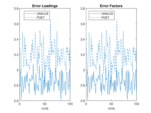
Figure 1: Bartlett’s estimates: $Loss_{B}$, $Loss_{f}$ for Setting 1 over $100$ replicates.

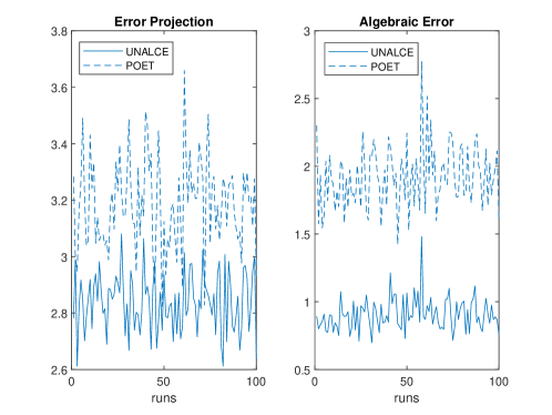
Figure 2: Bartlett’s estimates: $Loss_{Bf}$ and $PrErr$ for Setting 1 over $100$ replicates.

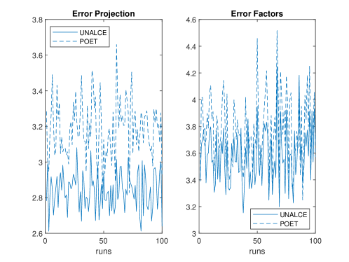
Figure 3: Bartlett’s estimates: $Loss_{B}$, $Loss_{f}$ for Setting 4 over $100$ replicates.

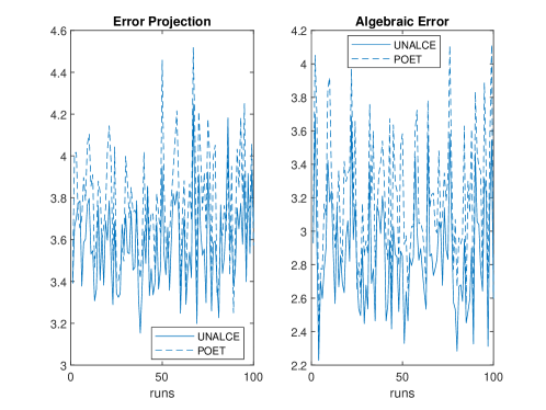
Figure 4: Bartlett’s estimates: $Loss_{Bf}$ and $PrErr$ for Setting 4 over $100$ replicates.

8 A real data example

In this section, we apply the UNALCE methodology to a real financial dataset, already used in Fan et al. (2013) to describe the performance of POET methodology. The dataset contains $251$ annualized daily returns (year $2010$) of $p=50$ stocks, relative to five UK industry sectors: ”consumer goods-textiles and apparel clothing”, ”financial-credit services”, ”healthcare-hospitals”, ”services-restaurant” and ”utilities-water utilities”, with $10$ stocks from each sector.

In Figure 5, we report the eigenvalues of the $50-$dimensional sample covariance matrix. Looking at the figure from a factor model perspective, we can state that no more than $3$ latent factors should be considered.

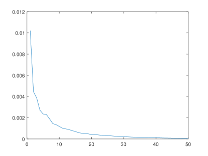
Figure 5: Sample eigenvalues: UK market data

In Fan et al. (2013), the authors show the results of POET methodology with $r=2$, reporting that $25.8\%$ of recovered residual non-zeros are within blocks, and $6.7\%$ are off-blocks. In addition, all recovered non-zeros are positive within blocks, while only $60.3\%$ are positive off-blocks. The results are claimed to be similar for $r=1,2,3$.

In order to make a comparison, we have computed UNALCE estimates for a grid of $20\times 20$ thresholds. The statistics of the optimal solutions, recovered via MC criterion (see Farnè and Montanari (2020)), are reported in Table 7 (the optimal thresholds are $\widehat{\psi}=0.0007$ and $\widehat{\rho}=0.0004$). We can note that the recovered rank is $1$, the UNALCE proportion of latent variance is very low (under $20\%$), and the recovered residual is diagonal.

Since UNALCE, differently from POET, recovers exactly the rank and the sparsity pattern, we have computed POET solutions (with hard thresholding) for $r=1$, selecting via $10-$fold cross-validation the optimal constant $\widehat{C}=1.10$ over a grid of $1000$ constants, linearly spaced from $0$ to $100$. The results are reported in Table 7. We can note that the latent variance proportion is still very low ($23.29\%$), and the residual presents a relevant proportion of off-diagonal non-zeros ($19\%$) but a very small proportion of residual covariance ($0.89\%$). This means that the recovered non-zeros are irrelevant to explain the covariance structure. What is more, only $10.2\%$ of within-blocks elements are non-zeros, against the $21\%$ of off-blocks elements, and all recovered non-zeros are positive.

Table 7: Covariance estimation results for UNALCE and POET (with $r=1$). $\widehat{r}$ is the latent rank, $\widehat{\theta}$ is the latent variance proportion, $\widehat{\rho}_{\widehat{S}}$ is the residual covariance proportion, $\widehat{\pi}_{nz}$ is the residual nonzero proportion, $\|\widehat{\Sigma}-\Sigma_{n}\|$ is the sample total loss.

	UNALCE	POET
$\widehat{r}$	1	1
$\widehat{\theta}$	0.1930	0.2329
$\widehat{\rho}_{\widehat{S}}$	0	0.0089
$\widehat{\pi}_{nz}$	0	0.1902
$\|\widehat{\Sigma}-\Sigma_{n}\|$	0.0013	0.0021

Since we know that POET does not offer any algebraic guarantee on the recovered sparsity pattern, and UNALCE approximates quite better the sample covariance matrix (the sample total loss is $0.0013$ against $0.0021$ for POET), we cannot claim so easily the presence of a residual cluster-wise structure. On the contrary, it is more likely that we have one weak latent factor (consistently recovered by UNALCE) which entirely explains the covariance structure. The result reported in Fan et al. (2013) could be explained by the use of principal component analysis with $p=50$, which could be not large enough to ensure that the estimated residuals are no longer correlated across variables.

Finally, we calculate three quantities to estimate the variability of the estimated loadings, factor scores and factor projections:

• $var_{B}=\sum_{j=1}^{p}\|\widehat{b}_{j}-\tilde{b}\|$, where $\tilde{b}$ is the mean estimated factor loading;

• $var_{f}=\sum_{k=1}^{n}\|\widehat{f}_{k}\|$ for factor scores ($\sum_{k=1}^{n}{\widehat{f}_{k}}$ is zero by construction);

• $var_{Bf}=\sum_{k=1}^{n}\|\widehat{B}\widehat{f}_{k}-\widetilde{Bf}\|$, where $\widetilde{Bf}$ is the mean factor projection across the observations.

These computations are reported for Bartlett’s and Thompson’s UNALCE and POET factor model estimates in Table 8. We observe that $var_{B}$ and $var_{Bf}$ are better for UNALCE, as we could expect from Corollary 1 and Theorems 1 and 2, while $var_{f}$ presents smaller values for POET. This is due to the particular structure of the POET residual component, which presents only positive elements. However, we must note that such structure cannot be trusted, as UNALCE recovers a diagonal residual and possesses the algebraic consistency property.

Table 8: Estimated variabilities for UNALCE and POET ($r=1$). Bartlett’s and Thompson’s factor loadings, scores and projections.

Metric	Method	UNALCE	POET
$var_{B}$		0.1990	0.2367
$var_{f}$	Bartlett	197.53	194.25
	Thompson	189.74	174.65
$var_{Bf}$	Bartlett	18.17	19.63
	Thompson	17.46	17.65

9 Conclusions

In this paper, we propose a new method to estimate an approximate factor model with a sparse residual in high dimensions. In particular, we elaborate over the results of Farnè and Montanari (2020) to prove that the ordinary least squares (OLS) estimates of factor loadings and scores based on UNALCE (UNshrunk ALgebraic Covariance Estimator) are asymptotically consistent, as well as the same estimates based on POET (Fan et al., 2013). Consistency holds in Euclidean norm under the assumption of intermediate spikiness of latent eigenvalues and element-wise sparsity of the residual component, while UNALCE provides the exact recovery of the latent rank and the residual sparsity pattern. A lower bound is imposed on the smallest latent eigenvalue and the smallest absolute nonzero residual element to ensure identifiability.

Moving from the eigenvalue dispersion lemma of Ledoit and Wolf (2004), we then prove that Bartlett’s and Thompson’s factor scores show the tightest possible error bound in Euclidean norm given the finite sample, within the class of estimate pairs with exact low rank and sparsity pattern. The proofs require advanced techniques of matrix algebra. In addition, it is proved that the projection of the low rank error matrix onto the orthogonal complement of the low rank space has the minimum possible Euclidean norm given the finite sample. Moreover, Bartlett’s and Thompson’s scores converge to the OLS ones, thus being also asymptotically consistent.

In the end, we prove in an ad hoc simulation study the validity of our optimality results, showing that UNALCE-based factor scores work particularly well with respect to POET-based ones if the latent eigenvalues are not so spiked and the residual is very sparse with prominent non-zeros in absolute value. A real financial data example further supports the optimality properties of the UNALCE approach compared to the POET one.

Appendix A Assumptions and key results of Farnè and Montanari (2020)

A.1 Assumptions

Assumption 1.

All the eigenvalues of the $r\times r$ matrix $p^{-\alpha}\mathbf{B}^{\top}\mathbf{B}$ are bounded away from $0$ for all $p$ and $\alpha\in[0,1]$.

Assumption 2.

There exist $k_{L},k_{S}>0$, $\delta\in[0,0.5]$, such that $\xi(T(\mathbf{L}^{*}))=\sqrt{{r}/{(k_{L}^{2}p^{2\delta})}}$, $\mu(\Omega(\mathbf{S}^{*}))=k_{S}p^{\delta}$, ${k_{S}}/{k_{L}}\leq{1}/{54}$ with $\delta<\alpha$.

Assumption 3.

There exist $r_{1},r_{2}>0$ and $b_{1},b_{2}>0$ such that, for any $t>0$, $k\leq n$, $i\leq r$, $j\leq p$:

$$\Pr(|\mathbf{f}_{ik}|>s)\leq\exp({-b_{1}/t}),\qquad\Pr(|\mathbf{\epsilon}_{jk}|>s)\leq\exp({-b_{2}/t}).$$

Assumption 4.

There exist $c_{1},c_{2},c_{3},\delta_{2},\delta_{2}^{\prime}>0$, $\delta^{\prime}\in[0,\delta+0.5]$ such that $\lambda(\mathbf{S}^{*})_{min}>c_{1}$, $\min_{i,j\leq p}\mathrm{var}(\mathbf{\epsilon}_{ik}\mathbf{\epsilon}_{jk})>c_{2}$ for any $k\leq n$, $i,j\leq p$, $s^{*}_{ii}\leq c_{3}$ for any $i\leq p$,$s^{\prime}=\max_{i\leq p}\sum_{j\leq p}\mathbbm{1}(\mathbf{S}^{*}_{ij}=0)\leq\delta_{2}p^{\delta}$ with $\delta_{2}\geq k_{S}$ and $\|\mathbf{S}\|_{1,v}=\max_{i\leq p}\sum_{j\leq p}|\mathbf{S}^{*}_{ij}|\leq\delta_{2}^{\prime}p^{\delta^{\prime}}$.

Assumption 5.

There exist $\delta_{3},\delta_{4}>0$ such that $r=\delta_{3}\ln{p}$ and $n\geq\delta_{4}p^{1.5\delta}$.

Assumption 6.

$2\delta\leq\alpha\leq 2\delta+\delta^{\prime}$ and $\delta_{5}<\frac{C_{3}\delta}{k_{L}\delta_{4}}<\delta^{\prime}$ with $\delta_{5}>0$.

Assumption 1 prescribes that the latent eigenvalues are spiked in the sense of Yu and Samworth (Fan et al. (2013), p. 656), thus allowing for intermediately pervasive latent factors as $p$ diverges. Assumption 2 ensures the identifiability of $L^{*}$ and $S^{*}$. Note that the condition $\delta<\alpha$ imposes a gap between the magnitude of latent eigenvalues and the residual sparsity degree, i.e. the number of residual non-zeros. Assumption 3 bounds the tails of factors and residuals. Assumption 4 controls for the sparsity degree of the residual component. Assumption 5 prescribes the order of the latent rank and a necessary lower bound for the sample size. Assumption 6 ensures the sparsity pattern recovery. We refer to Farnè and Montanari (2020) for more details.

A.2 Key results

Theorem 1.

Let $\Omega=\Omega({S}^{*})$ and $T=T({L}^{*})$. Suppose that Assumptions 1-6 and Assumption 1 hold. Define

$$\psi=\frac{1}{\xi(T)}\frac{p^{\alpha}}{\sqrt{n}}$$

with $\rho=\gamma\psi$, where $\gamma\in[9\xi(T),1/(6\mu(\Omega))]$. Then, with probability greater than $1-C_{4}p^{-C_{5}}$, the pair $(\widehat{{L}},\widehat{{S}})$ minimizing (6) recovers the rank of ${L}^{*}$ ($rank(\widehat{{L}})=rank({L}^{*})$) and the sparsity pattern of $S^{*}$ ($sign(\widehat{{S}})=sign({S}^{*})$). Moreover, the matrix losses for each component are bounded as follows:

$$\|\widehat{{L}}-{L}^{*}\|_{2}\leq C\psi,\qquad\|\widehat{{S}}-{S}^{*}\|_{\infty}\leq C\rho.$$

Once defined $\phi_{S}=Cs^{\prime}\xi(T)\psi$ and $\phi=C(s^{\prime}\xi(T)+1)\psi$, where $s^{\prime}$ is the maximum number of non-zeros per row/column in ${S}^{*}$, we can state the following Corollary.

Corollary 1.

Under the assumptions of Theorem 1, it holds $||\widehat{{S}}_{ALCE}-{S}^{*}||_{2}\leavevmode\nobreak\ \leq\phi_{S}$, $||\widehat{{\Sigma}}_{ALCE}-{\Sigma}^{*}||_{2}\leq\phi$, $||\widehat{{S}}_{ALCE}^{-1}-{S}^{*-1}||_{2}\leq\phi_{S}$, and $||\widehat{{\Sigma}}_{ALCE}^{-1}-{\Sigma}^{{}^{*}-1}||_{2}\leq\psi$. In addition, $\widehat{{S}}_{ALCE}$, $\widehat{{\Sigma}}_{ALCE}$, $\widehat{{S}}_{ALCE}^{-1}$, $\widehat{{\Sigma}}_{ALCE}^{-1}$ are positive definite if and only if $\lambda_{p}({{S}^{*}})>\phi_{{S}}$, $\lambda_{p}({{\Sigma}^{*}})>\phi$, $\lambda_{p}({{S}^{*}})\geq 2\phi_{{S}}$, $\lambda_{p}({{\Sigma}^{*}})\geq 2\phi$, respectively.

We refer to Farnè and Montanari (2020) for the proofs.

Appendix B Proofs

B.1 Proof of Theorem 1

Recalling that ${\Sigma}_{n}=(n-1)^{-1}\sum_{k=1}^{n}{x}_{k}{x}_{k}^{\prime}$ and ${x}_{k}={B}{f}_{k}+{\epsilon}_{k}$, where ${{f}}_{k}$ and ${{\epsilon}}_{k}$, $k=1,\ldots,n$, are respectively the vectors of factor scores and residuals for each observation, we can decompose the error matrix ${{E}}_{n}={\Sigma}_{n}-{\Sigma}^{*}$ in four components as follows (cf. Fan et al. (2013)):

$${{E}}_{n}={\Sigma}_{n}-{\Sigma}^{*}=\widehat{{D}}_{1}+\widehat{{D}}_{2}+\widehat{{D}}_{3}+\widehat{{D}}_{4},$$

where:

$$\widehat{{D}}_{1}=\left(n^{-1}{B}\sum_{k=1}^{n}{f}_{k}{f}_{k}^{\prime}-{I}_{r}\right){B}^{\prime},\widehat{{D}}_{2}=n^{-1}\sum_{k=1}^{n}\left({\epsilon}_{k}{\epsilon}_{k}^{\top}-{S}^{*}\right),\widehat{{D}}_{3}=n^{-1}{B}\sum_{k=1}^{n}{f}_{k}{\epsilon}_{k}^{\prime},\widehat{{D}}_{4}=\widehat{{D}}_{3}^{\prime}.$$

We thus recall from Farnè and Montanari (2020) the following result.

Lemma 1.

Under Assumptions 1, 3, 4, 5, there exists a positive constant $C$ such that

$$||{D}_{1}||_{2} \leq C\left(p^{\alpha}\sqrt{\frac{1}{n}}\right);$$

$$||{D}_{2}||_{2} \leq C\left(p^{\delta}\sqrt{\frac{\log{p}}{n}}\right);$$

$$||{D}_{3}||_{2} \leq C\left(p^{\frac{\alpha}{2}+\frac{\delta}{2}}\sqrt{\frac{\log{p}}{n}}\right).$$ (14)

As a consequence, we can recall the following fundamental Lemma proved in Farnè and Montanari (2020).

Lemma 2.

Let $\widehat{\lambda}_{r}$ be the $r-$th largest eigenvalue of ${{\Sigma}}_{n}$. Under the assumptions of Lemma 1, if $\delta<\alpha$, then $\widehat{\lambda}_{r}>C_{1}p^{\alpha}$ with probability approaching $1$ for some $C_{1}>0$.

Then, we proceed as follows. According to Bai (2003), setting $\widehat{F}=\widehat{F}_{OLS,1}$, we can write, for each $t=1,\ldots,n$,

$$\widehat{f}_{t}-Hf_{t}=\left(\frac{\widehat{\Lambda}_{r}}{p}\right)^{-1}\left\{\frac{1}{n}\sum_{s=1}^{n}\widehat{f}_{s}\frac{E(\epsilon_{s}^{\prime}\epsilon_{t})}{p}+\frac{1}{n}\sum_{s=1}^{n}\widehat{f}_{s}\varsigma_{st}+\frac{1}{n}\sum_{s=1}^{n}\widehat{f}_{s}\eta_{st}+\frac{1}{n}\sum_{s=1}^{n}\widehat{f}_{s}\xi_{st}\right\},$$

where $\xi_{st}=\frac{(f_{t}^{\prime}\sum_{i=1}^{p}b_{i}\epsilon_{is})}{p}$, $\eta_{st}=\frac{(f_{s}^{\prime}\sum_{i=1}^{p}b_{i}\epsilon_{it})}{p}$, $\varsigma_{st}=\frac{\epsilon_{s}^{\prime}\epsilon_{t}}{p}-\frac{E(\epsilon_{s}^{\prime}\epsilon_{t})}{p}$, and $\widehat{\Lambda}_{r}$ is the diagonal matrix containing the top $r$ eigenvalues of $\Sigma_{n}$ in decreasing order. The eigenvalues of $\left(\frac{\widehat{\Lambda}_{r}}{p}\right)^{-1}$ scale to $O(p^{1-\alpha})$ as $p\rightarrow\infty$.

Relying on Assumption 2, we can prove the following lemmas by simply applying the corresponding proofs in Fan et al. (2013), where Assumption 2 is imposed with $\alpha=1$.

Lemma 3.

For all $i\leq r$:

$$\frac{1}{n}\sum_{t=1}^{n}\left(\frac{1}{np}\sum_{s=1}^{n}\widehat{f}_{is}E(\epsilon_{s}^{\prime}\epsilon_{t})\right)^{2} = O(n^{-1});$$

$$\frac{1}{n}\sum_{t=1}^{n}\frac{1}{n}\left(\sum_{s=1}^{n}\widehat{f}_{is}\varsigma_{st}\right)^{2} = O(p^{-\alpha});$$

$$\frac{1}{n}\sum_{t=1}^{n}\frac{1}{n}\left(\sum_{s=1}^{n}\widehat{f}_{is}\eta_{st}\right)^{2} = O(p^{-\alpha});$$

$$\frac{1}{n}\sum_{t=1}^{n}\frac{1}{n}\left(\sum_{s=1}^{n}\widehat{f}_{is}\xi_{st}\right)^{2} = O(p^{-\alpha}).$$

Lemma 4.

$$\max_{t\leq n}\bigg{|}\bigg{|}\frac{1}{np}\sum_{s=1}^{n}\widehat{f}_{s}E(\epsilon_{s}^{\prime}\epsilon_{t})\bigg{|}\bigg{|}=O\left(\sqrt{\frac{1}{n}}\right);$$

$$\max_{t\leq n}\bigg{|}\bigg{|}\frac{1}{n}\sum_{s=1}^{n}\widehat{f}_{s}\varsigma_{st}\bigg{|}\bigg{|}=O\left(\frac{n^{1/4}}{p^{\alpha/2}}\right);$$

$$\max_{t\leq n}\bigg{|}\bigg{|}\frac{1}{n}\sum_{s=1}^{n}\widehat{f}_{s}\eta_{st}\bigg{|}\bigg{|}=O\left(\frac{n^{1/4}}{p^{\alpha/2}}\right);$$

$$\max_{t\leq n}\bigg{|}\bigg{|}\frac{1}{n}\sum_{s=1}^{n}\widehat{f}_{s}\xi_{st}\bigg{|}\bigg{|}=O\left(\frac{n^{1/4}}{p^{\alpha/2}}\right).$$

We recall that $H=\frac{1}{n}(\widehat{\Lambda}_{r})^{-1}\widehat{F}^{\prime}FB^{\prime}B$. Since the eigenvalues of $\left(\frac{\widehat{\Lambda}_{r}}{p}\right)^{-1}$ scale to $O(p^{1-\alpha})$ instead of $O(p)$, applying Assumption 2 and following Fan et al. (2013) we obtain

Lemma 5.

$$\max_{i\leq r}\frac{1}{n}\sum_{k=1}^{n}(\widehat{f}_{k}-Hf_{k})_{i}^{2}=O\left(\frac{p^{1-\alpha}}{n}+\frac{p^{1-\alpha}}{p^{\alpha}}\right);$$

$$\frac{1}{n}\sum_{k=1}^{n}||\widehat{f}_{k}-Hf_{k}||=O\left(\frac{p^{1-\alpha}}{n}+\frac{p^{1-\alpha}}{p^{\alpha}}\right);$$

$$\max_{k\leq n}\sum_{k=1}^{n}||\widehat{f_{k}}-Hf_{k}||=O\left({\frac{p^{1-\alpha}}{\sqrt{n}}}+\frac{p^{1-\alpha}n^{1/4}}{p^{\alpha/2}}.\right)$$ (15)

Note that (15), which bounds the uniform rate of $\widehat{f}_{k}-Hf_{k}$ over $k=1,\ldots,n$, proves the second thesis of Theorem 1.

At the same time, applying Assumption 2 and following Fan et al. (2013), we can claim

Lemma 6.

$$HH^{\prime}=I_{\widehat{r}}+O\left(\frac{p^{(1-\alpha)/2}}{\sqrt{n}}+\frac{p^{(1-\alpha)/2}}{p^{\alpha/2}}\right);$$

$$H^{\prime}H=I_{{r}}+O\left(\frac{p^{(1-\alpha)/2}}{\sqrt{n}}+\frac{p^{(1-\alpha)/2}}{p^{\alpha/2}}\right).$$

We can now prove the first thesis of Theorem 1, about the uniform rate of $\widehat{b}_{j}-Hb_{j}$ over $j=1,\ldots,p$. Following Fan et al. (2013), we know that $\widehat{b}_{j}-Hb_{j}$ can be decomposed in three terms:

$$\widehat{b}_{j}-Hb_{j}=\frac{1}{n}\sum_{k=1}^{n}Hf_{k}\epsilon_{k,i}+\sum_{k=1}^{n}x_{k,i}(\widehat{f}_{k}-Hf_{k})+H(\widehat{f}_{k}\widehat{f}_{k}^{\prime}-I_{r})b_{j}=I+II+III.$$ (16)

The claim (14) in Lemma 1 allows us to prove that $I$ is $O\left(p^{\delta/2}\sqrt{\frac{\log(p)}{n}}\right)$. From Lemma 5 and the fact $||H||=O(1)$, it follows that the $II$ is $O\left(\frac{p^{\frac{1-\alpha}{2}}}{n^{\frac{1}{2}}}+\frac{p^{\frac{1-\alpha}{2}}}{p^{\frac{\alpha}{2}}}\right)$. Lemma 5 and Assumption 2 imply that $III$ is $O\left(\frac{1}{\sqrt{n}}\right)$. Therefore, we can prove that

$$\max_{j\leq p}||{\widehat{b}_{j}-Hb_{j}}||=O_{p}\left(\omega_{n}\right)$$

where $\omega_{n}=p^{\delta/2}\sqrt{\frac{\log p}{n}}+\frac{p^{(1-\alpha)/2}}{p^{\alpha/2}}$.

Applying the two proved theses of Theorem 1 and Lemma 6, we can consequently prove, for each $k=1,\ldots,n$, the third thesis:

$$\max_{j\leq p,i\leq r}||\widehat{b}_{j}^{\prime}\widehat{f}_{k}-b_{j}^{\prime}f_{k}||=O\left(\frac{n^{1/4}p^{1-\alpha}}{p^{\alpha/2}}+\log(n)^{1/b_{2}}p^{\delta/2}\sqrt{\frac{\log{p}}{n}}\right)$$ (17)

simply following Fan et al. (2013).

B.2 Proof of Theorem 2

Corollary 1 in Farnè and Montanari (2020) prescribe that $\widehat{L}_{ALCE}=\widehat{U}_{ALCE}\widehat{D}_{ALCE}\widehat{U}_{ALCE}^{\prime}$ is asymptotically consistent if and only if $p^{\alpha+\delta}/n$ tends to $0$ as both $p$ and $n$ diverge. Therefore, as these conditions are respected, $\widehat{L}_{ALCE}$ and $\widehat{L}_{POET}$ both converge to $L^{*}$, and the proof of Theorem 1 can be straightforwardly applied to UNALCE estimates taking into account that now $\left(\frac{\widehat{D}_{ALCE}}{p}\right)^{-1}$ scale to $O(p^{1-\alpha-\delta})$ instead of $O(p^{1-\alpha})$.

B.3 Proof of Theorem 1

Let us decompose the minimization problems considered in Theorem 1 conditioning on $Y_{pre}$ and $Z_{pre}$. Suppose that the assumptions of Theorem 1 hold. The problem in $L$ can be rewritten as

$$\min_{L\in\widehat{\mathcal{B}}(\widehat{r})}||L-L^{*}||^{2}=\min_{L\in\widehat{\mathcal{B}}(\widehat{r})}||L-Y_{pre}+Y_{pre}-L^{*}||^{2}\leq\min_{L\in\widehat{\mathcal{B}}(\widehat{r})}||L-Y_{pre}||^{2}+||Y_{pre}-L^{*}||^{2},$$

which is minimum if $L=\widehat{L}_{UNALCE}$ because of the optimal approximation property of principal components, since $\widehat{L}_{UNALCE}$ is derived by the top $\widehat{r}$ principal components of ${Y}_{pre}$.

The problem in $S$ can be rewritten as follows. Suppose that, exploiting the assumption $diag(L)+diag(S)=diag(\widehat{\Sigma}_{ALCE})$, we constrain ourselves within the class of matrices with diagonal $diag(\widehat{\Sigma}_{ALCE})-diag(L)$, where $L$ has rank at most $r$ and belongs to $\widehat{\mathcal{B}}(\widehat{r})$. We call this space $\widehat{\mathcal{A}}_{diag}$. Defining ${\Sigma}_{pre}={Y}_{pre}+{Z}_{pre}$, conditioning on $Y_{pre}$ and assuming the invariance of the off-diagonal elements in $\widehat{S}$, we can write

$$\min_{S\in\widehat{\mathcal{A}}_{diag}}||S-S^{*}||^{2}=\min_{L\in\widehat{\mathcal{B}}(\widehat{r})}||(\widehat{\Sigma}_{ALCE}-L)-(\Sigma_{pre}-Y_{pre})+(\Sigma_{pre}-Y_{pre})-(\Sigma^{*}-L^{*})||\leq$$

$$\min_{L\in\widehat{\mathcal{B}}(\widehat{r})}||(\widehat{\Sigma}_{ALCE}-L)-(\Sigma_{pre}-Y_{pre})||+||(\Sigma_{pre}-Y_{pre})-(\Sigma^{*}-L^{*})||\leq$$

$$\min_{L\in\widehat{\mathcal{B}}(\widehat{r})}||(\widehat{\Sigma}_{ALCE}-\Sigma_{pre})||+||L-Y_{pre}||+||(\Sigma_{pre}-Y_{pre})-(\Sigma^{*}-L^{*})||.$$

Since $(\widehat{\Sigma}_{ALCE}-\Sigma_{pre})$ and $(\Sigma_{pre}-Y_{pre})-(\Sigma^{*}-L^{*})$ are fixed, the entire problem boils down to $\min_{L\in\widehat{\mathcal{B}}(\widehat{r})}||L-Y_{pre}||^{2}$, which is solved for $L=\widehat{L}_{UNALCE}$. Therefore, we can write $\widehat{S}_{UNALCE}=\min_{S\in\widehat{\mathcal{A}}_{diag}}||S-S^{*}||^{2}$, and the minimum amounts to $||\widehat{S}_{UNALCE}-S^{*}||^{2}$.

The problem in $\Sigma$ can be rewritten as

$$\min_{\Sigma\in\widehat{Y}}||\Sigma-\Sigma^{*}||=\min_{\Sigma\in\widehat{Y}}||L-L^{*}+S-S^{*}||\leq$$

$$\leq\min_{L\in\widehat{\mathcal{B}}(\widehat{r})}||L-L^{*}||+\min_{S\in\widehat{\mathcal{A}}_{diag}}||S-S^{*}||\leq\min_{L\in\widehat{\mathcal{B}}(\widehat{r})}||L-Y_{pre}||+||Y_{pre}-L^{*}||+||\widehat{S}_{UNALCE}-S^{*}||$$

or alternatively

$$\leq\min_{L\in\widehat{\mathcal{B}}(\widehat{r})}2||L-Y_{pre}||+||Y_{pre}-L^{*}||+||(\widehat{\Sigma}_{ALCE}-\Sigma_{pre})||+||(\Sigma_{pre}-Y_{pre})-(\Sigma^{*}-L^{*})||$$

which is minimum if $L=\widehat{L}_{UNALCE}$ and $S=\widehat{S}_{UNALCE}$.

The same optimality properties are transmitted to $S^{*-1}$ and $\Sigma^{*-1}$. It is enough to recall that

$$||\widehat{S}^{-1}-S^{*-1}||\leq||{S}^{*-1}||\times||\widehat{S}-S^{*}||\times||{S}^{*-1}||\leq 2\lambda_{min}(S^{*})||\widehat{S}-S^{*}||$$

and

$$||\widehat{\Sigma}^{-1}-\Sigma^{*-1}||\leq||{\Sigma}^{*-1}||\times||\widehat{\Sigma}-\Sigma^{*}||\times||{\Sigma}^{*-1}||\leq 2\lambda_{min}(\Sigma^{*})||\widehat{\Sigma}-\Sigma^{*}||,$$

such that $\widehat{S}_{UNALCE}^{-1}$ and $\widehat{\Sigma}_{UNALCE}^{-1}$ minimize $||\widehat{S}^{-1}-S^{*-1}||$ and $||\widehat{\Sigma}^{-1}-\Sigma^{*-1}||$ respectively under the assumptions of Theorem 1.

B.4 Proof of Corollary 1

In order to prove the first part of the corollary, we can state that

$$||\mathbb{P}_{T^{\prime\perp}}(\widehat{L}_{UNALCE}-L^{*})||\leq||(\widehat{L}_{UNALCE}-L^{*})||\leq$$

$$||(\widehat{L}_{UNALCE}-\widehat{L}_{ALCE}+\widehat{L}_{ALCE}-L^{*})||\leq$$

$$||(\widehat{L}_{ALCE}-L^{*})||+||(\widehat{L}_{UNALCE}-\widehat{L}_{ALCE})||\leq(C+1)\psi,$$

where $C\geq\xi(T)$, because $\widehat{L}_{UNALCE}=\widehat{U}_{ALCE}(\widehat{D}_{ALCE}+\lambda I_{r})\widehat{U}_{ALCE}^{\prime}=\widehat{L}_{ALCE}+\widehat{U}_{ALCE}\lambda I_{r}\widehat{U}_{ALCE}^{\prime}$. Relying on $\widehat{S}_{UNALCE}=\widehat{S}_{ALCE}-diag(\widehat{U}_{ALCE}(\widehat{D}_{ALCE}+\lambda I_{r})\widehat{U}_{ALCE})$, we then have

$$g_{\gamma}(\widehat{\Sigma}_{UNALCE}-\Sigma^{*},\widehat{\Sigma}_{UNALCE}-\Sigma^{*})=||\widehat{\Sigma}_{UNALCE}-\widehat{\Sigma}_{ALCE}+\widehat{\Sigma}_{ALCE}-\Sigma^{*}||\leq$$

$$||\widehat{\Sigma}_{UNALCE}-\widehat{\Sigma}_{ALCE}||+||\widehat{\Sigma}_{ALCE}-\Sigma^{*}||\leq$$

$$||\widehat{L}_{UNALCE}-\widehat{L}_{ALCE}||+||\widehat{S}_{UNALCE}-\widehat{S}_{ALCE}||+||\widehat{\Sigma}_{ALCE}-\Sigma^{*}||=$$

$$|\widehat{U}_{ALCE}(\lambda I_{r})\widehat{U}_{ALCE}||+||-\widehat{U}_{ALCE}(\lambda I_{r})\widehat{U}_{ALCE}||+||\widehat{\Sigma}_{ALCE}-\Sigma^{*}||=$$

$$(C+2)\lambda,$$

with $C\leq 11$ (see Luo (2011)).

In order to prove the second part of the corollary, we recall from Farnè and Montanari (2020) that $||\widehat{L}_{ALCE}-Y_{pre}||-||\widehat{L}_{UNALCE}-Y_{pre}||\leq\psi$ and $||\widehat{\Sigma}_{ALCE}-\Sigma_{pre}||-||\widehat{\Sigma}_{UNALCE}-\Sigma_{pre}||\leq\psi$. Then we can write

$$||\mathbb{P}_{T^{\prime\perp}}(\widehat{L}_{ALCE}-Y_{pre}+Y_{pre}-L^{*})||\leq$$

$$||(\widehat{L}_{ALCE}-Y_{pre}+Y_{pre}-L^{*})||\leq$$

$$||\widehat{L}_{UNALCE}-\widehat{L}_{ALCE}||+||(\widehat{L}_{UNALCE}-Y_{pre})||+||(Y_{pre}-L^{*})||$$

Therefore,

$$||\mathbb{P}_{T^{\prime\perp}}(\widehat{L}_{ALCE}-L^{*})|-||\mathbb{P}_{T^{\prime\perp}}(\widehat{L}_{UNALCE}-L^{*})||\leq$$

$$||(\widehat{L}_{ALCE}-L^{*})||-||(\widehat{L}_{UNALCE}-L^{*})||\leq\psi.$$

Similarly, conditioning on $\Sigma_{pre}$ and recalling Farnè and Montanari (2020), we have

$$g_{\gamma}(\widehat{\Sigma}_{ALCE}-\Sigma^{*},\widehat{\Sigma}_{ALCE}-\Sigma^{*})-g_{\gamma}(\widehat{\Sigma}_{UNALCE}-\Sigma^{*},\widehat{\Sigma}_{UNALCE}-\Sigma^{*})\leq$$

$$||\widehat{\Sigma}_{ALCE}-\Sigma^{*}||-||\widehat{\Sigma}_{UNALCE}-\Sigma^{*}||\leq\psi.$$

B.5 Proof of Theorem 1

Restricting to $\widehat{\mathcal{Y}}=\widehat{\mathcal{B}}(\widehat{r})+\widehat{\mathcal{A}}(\widehat{s})$ and conditioning on $Y_{pre}$ and $Z_{pre}$ (which in turn rely on $\Sigma_{n}$), we have proved in Theorem 1 that $\widehat{L}_{UNALCE}=\min_{L\in\widehat{\mathcal{B}}(\widehat{r})}||L-L^{*}||^{2}$, $\widehat{S}_{UNALCE}=\min_{S\in\widehat{\mathcal{A}}(\widehat{s})}||S-S^{*}||^{2}$ and $\widehat{\Sigma}_{UNALCE}=\min_{\Sigma\in\widehat{Y}}||\Sigma-\Sigma^{*}||^{2}$. According to Ledoit and Wolf (2004), we can write

$$\frac{1}{p}E\left[\sum_{i=1}^{p}(\widehat{\lambda}_{L,i}-\mu_{L})^{2}|\Sigma_{n}\right]=\frac{1}{p}\sum_{i=1}^{p}(\lambda_{L,i}-\mu_{L})^{2}+E(||\widehat{L}-L^{*}||^{2}|\Sigma_{n}),$$ (18)

$$\frac{1}{p}E\left[\sum_{i=1}^{p}(\widehat{\lambda}_{S,i}-\mu_{S})^{2}|\Sigma_{n}\right]=\frac{1}{p}\sum_{i=1}^{p}(\lambda_{S,i}-\mu_{S})^{2}+E(||\widehat{S}-S^{*}||^{2}|\Sigma_{n}),$$ (19)

$$\frac{1}{p}E\left[\sum_{i=1}^{p}(\widehat{\lambda}_{\Sigma,i}-\mu_{\Sigma})^{2}|\Sigma_{n}\right]=\frac{1}{p}\sum_{i=1}^{p}(\lambda_{\Sigma,i}-\mu_{L})^{2}+E(||\widehat{\Sigma}-\Sigma^{*}||^{2}|\Sigma_{n}),$$ (20)

where $\mu_{L}=tr({L}^{*})/p$, $\mu_{S}=tr({S}^{*})/p$ and $\mu_{\Sigma}=tr({\Sigma}^{*})/p$. As a consequence, since $E(||\widehat{L}\leavevmode\nobreak\ -\leavevmode\nobreak\ L^{*}||^{2}|\Sigma_{n})$, $E(||\widehat{S}-S^{*}||^{2}|\Sigma_{n})$ and $E(||\widehat{\Sigma}-\Sigma^{*}||^{2}|\Sigma_{n})$ are minimum under the assumptions of Theorem 1, we can write $\widehat{L}_{UNALCE}=\min_{L\in\widehat{\mathcal{B}}(\widehat{r})}\frac{1}{p}E\left[\sum_{i=1}^{p}(\widehat{\lambda}_{L,i}-\mu_{L})^{2}\right]$, $\widehat{S}_{UNALCE}=\min_{S\in\widehat{\mathcal{A}}_{diag}}\frac{1}{p}E\left[\sum_{i=1}^{p}(\widehat{\lambda}_{S,i}-\mu_{S})^{2}\right]$ and $\widehat{\Sigma}_{UNALCE}=\min_{\Sigma\in\widehat{Y}}\frac{1}{p}E\left[\sum_{i=1}^{p}(\widehat{\lambda}_{\Sigma,i}-\mu_{\Sigma})^{2}\right]$. These results mean that within the classes of algebraically consistent estimates the eigenvalues of $\widehat{L}_{UNALCE}$, $\widehat{S}_{UNALCE}$, and $\widehat{\Sigma}_{UNALCE}$ are the most concentrated possible around their respective true means.

The optimality properties of the eigenvalues of $S^{*}$ and $\Sigma^{*}$ estimated by UNALCE are transmitted to $S^{*-1}$ and $\Sigma^{*-1}$. In fact, we know that $E(||\widehat{S}^{-1}\leavevmode\nobreak\ -\leavevmode\nobreak\ S^{*-1}||^{2}|\Sigma_{n})$ and $E(||\widehat{\Sigma}^{-1}\leavevmode\nobreak\ -\leavevmode\nobreak\ \Sigma^{*-1}||^{2}|\Sigma_{n})$ are the minimum possible under the assumptions of Theorem 1. Since it also holds

$$\frac{1}{p}E\left[\sum_{i=1}^{p}(\widehat{\lambda}_{S^{-1},i}-\mu_{S^{-1}})^{2}|\Sigma_{n}\right]=\frac{1}{p}\sum_{i=1}^{p}(\lambda_{S^{-1},i}-\mu_{S^{-1}})^{2}+E(||\widehat{S}^{-1}-S^{*-1}||^{2}|\Sigma_{n}),$$

$$\frac{1}{p}E\left[\sum_{i=1}^{p}(\widehat{\lambda}_{\Sigma^{-1},i}-\mu_{\Sigma^{-1}})^{2}|\Sigma_{n}\right]=\frac{1}{p}\sum_{i=1}^{p}(\lambda_{\Sigma^{-1},i}-\mu_{\Sigma^{-1}})^{2}+E(||\widehat{\Sigma}^{-1}-\Sigma^{*-1}||^{2}|\Sigma_{n}),$$

where $\mu_{S^{-1}}$ and $\mu_{\Sigma^{-1}}$ are the mean eigenvalues of $S^{*-1}$ and $\Sigma^{*-1}$, we are allowed to conclude that $\widehat{S}^{-1}_{UNALCE}=\min_{S\in\widehat{\mathcal{A}}_{diag}}\sum_{i=1}^{p}\widehat{S}^{-1}_{UNALCE}=(\widehat{\lambda}_{S^{-1},i}-\mu_{S^{-1}})^{2}$ and $\widehat{\Sigma}^{-1}_{UNALCE}=\min_{\Sigma\in\widehat{Y}}\sum_{i=1}^{p}(\widehat{\lambda}_{\Sigma^{-1},i}-\mu_{\Sigma^{-1}})^{2}$ .

B.6 Proof of Corollary 2

We show the proof with respect to $\widehat{L}_{UNALCE}$ as the extension to $\widehat{S}_{UNALCE}$, $\widehat{\Sigma}_{UNALCE}$, $\widehat{S}^{-1}_{UNALCE}$, $\widehat{\Sigma}^{-1}_{UNALCE}$ is straightforward. From Theorem 1 we know that

$$sum_{L}=\sum_{i=1}^{p}(\widehat{\lambda}_{\widehat{L}_{UNALCE},i}-\mu_{L})^{2}=$$

$$=\sum_{i=1}^{p}\widehat{\lambda}_{\widehat{L}_{UNALCE},i}^{2}+p\mu_{L}^{2}-2\mu_{L}\sum_{i=1}^{p}\widehat{\lambda}_{\widehat{L}_{UNALCE},i}$$

is minimum into the recovered low rank matrix variety. Then we note that $sum_{L}/p$ can be rewritten as $\frac{1}{p}tr(\widehat{L}_{UNALCE}-\mu_{L}I_{p})^{2}$. We know that $\frac{1}{p}(tr(\widehat{L}_{UNALCE}-\mu_{L}I_{p})^{2})$ is the second moment of $\rho(z)_{\widehat{L}_{UNALCE}-{L^{*}}}$, because $tr(\mu_{L}I_{p})=tr(L^{*})$ and $tr(\widehat{L}_{UNALCE}-\mu_{L}I_{p})^{2}=tr(\widehat{L}_{UNALCE}-L^{*})^{2}$. Therefore, the claim on the second moment of $\rho(z)_{\widehat{L}_{UNALCE}-L^{*}}^{p}$ is proved. Concerning the claim on the first moment of $\rho(z)_{\widehat{L}_{UNALCE}-L^{*}}$, it is sufficient to note that $tr(\widehat{L}_{UNALCE}-\mu_{L}I_{p})=tr(\widehat{L}_{UNALCE}-L^{*})$ tends to $0$ as $\psi=\frac{1}{\xi(T)}\frac{p^{\alpha}}{\sqrt{n}}$ tends to $0$.

B.7 Proof of Corollary 1

Since the eigenvalues of $\widehat{L}_{UNALCE}$ are the most concentrated around their mean under the assumptions of Theorem 1, the same holds for $\widehat{B}_{UNALCE}$, because its eigenvalues are the square root of the ones of $\widehat{L}_{UNALCE}$ and the variance is a monotonic operator. Therefore, according to Ledoit and Wolf (2004), $\min_{B,{L}={B}{B}^{\prime}\in\widehat{\mathcal{B}}}||\widehat{B}-B|||\Sigma_{n}$ is solved by $\widehat{B}=\widehat{B}_{UNALCE}$ under the constraint $\widehat{B}^{\prime}\widehat{B}$ diagonal and $\sum_{i=1}^{p}||\widehat{b}_{i}||=\max$.

B.8 Proof of Theorem 1

We start considering the loss $||\widehat{f}_{k,B}-f_{k,B}||$. Since $\widehat{f}_{k,B}=(\widehat{B}^{\prime}\widehat{S}^{-1}\widehat{B})^{-1}\widehat{B}^{\prime}\widehat{S}^{-1}x_{k}$, $k=1,\ldots,n$, that loss is majorized by $||(\widehat{B}^{\prime}\widehat{S}^{-1}\widehat{B})^{-1}\widehat{B}^{\prime}\widehat{S}^{-1}-(B^{\prime}S^{*-1}B)^{-1}B^{\prime}S^{*-1}||\times||x_{k}||$. The eigenvalues of $\widehat{B}^{\prime}\widehat{S}^{-1}\widehat{B}$ coincide with the ones of $\widehat{S}^{-1}\widehat{B}\widehat{B}^{\prime}=\widehat{S}^{-1}\widehat{L}$. According to Ledoit and Wolf (2004), the expected variance of the estimated eigenvalues around their true mean depends on the true variance and the squared bias in spectral norm of the overall estimate. Therefore, conditioning on $\Sigma_{n}$, we can focus on the spectral losses $||\widehat{B}^{\prime}\widehat{S}^{-1}-B^{\prime}S^{*-1}||$ and $||\widehat{S}^{-1}\widehat{L}-S^{*-1}L^{*}||$.

We first focus on $||\widehat{S}^{-1}\widehat{L}-S^{*-1}L^{*}||$. Conditioning on $Y_{pre}$ and $Z_{pre}$, we can write

$$||\widehat{S}^{-1}\widehat{L}-S^{*-1}L^{*}||\leq||\widehat{S}^{-1}\widehat{L}-Z_{pre}^{-1}Y_{pre}||+||Z_{pre}^{-1}Y_{pre}-S^{*-1}L^{*}||,$$

where the term $||Z_{pre}^{-1}Y_{pre}-S^{*-1}L^{*}||$ entirely depends on $\Sigma_{n}$.

We now consider two generic estimates $L$ and $S$. Under the assumptions of Theorem 1, we must constrain our search by setting $off-diag(S)=off-diag(\widehat{S}_{ALCE})$ and $diag(S)=diag(\widehat{\Sigma}_{ALCE}-L)$, $L\in\mathcal{L}(\widehat{r})$. Therefore, conditioning on ${\Sigma}_{pre}={Y}_{pre}+{Z}_{pre}$, we can write

$$||\widehat{S}^{-1}\widehat{L}-Z_{pre}^{-1}Y_{pre}||=||({\Sigma}_{pre}-L)^{-1}L-({\Sigma}_{pre}-Y_{pre})^{-1}Y_{pre}||,$$

with $off-diag(L)=off-diag({Y}_{pre})$. We apply the formula $({\Sigma}_{pre}-L)^{-1}=\sum_{k=0}^{\infty}({\Sigma}_{pre}^{-1}L)^{k}{\Sigma}_{pre}^{-1}$, which leads to

$$||({\Sigma}_{pre}-L)^{-1}L-({\Sigma}_{pre}-Y_{pre})^{-1}Y_{pre}||=\left|\left|\sum_{k=0}^{\infty}({\Sigma}_{pre}^{-1}L)^{k}{\Sigma}_{pre}^{-1}L-\sum_{k=0}^{\infty}({\Sigma}_{pre}^{-1}Y_{pre})^{k}{\Sigma}_{pre}^{-1}Y_{pre}\right|\right|.$$

Conditioning on $Y_{pre}$, we can write $L=Y_{pre}+\Delta_{L,pre}$. Therefore, it follows

$$||({\Sigma}_{pre}-L)^{-1}L-({\Sigma}_{pre}-Y_{pre})^{-1}Y_{pre}||=\left|\left|\sum_{k=0}^{\infty}\Sigma_{pre}^{-k}(L^{k}-Y_{pre}^{k}){\Sigma}_{pre}^{-1}\Delta_{L,pre}\right|\right|.$$

Applying Cauchy-Schwartz inequality, we obtain

$$\left|\left|({\Sigma}_{pre}-L)^{-1}L-({\Sigma}_{pre}-Y_{pre})^{-1}Y_{pre}\right|\right|\leq$$

$$\sum_{k=0}^{\infty}||{\Sigma}_{pre}^{-k}||\times||L^{k}-Y_{pre}^{k}||\times||{\Sigma}_{pre}^{-1}||\times||\Delta_{L,pre}||$$ (21)

Recalling Theorem 1, which states that the variance of the eigenvalues of $\widehat{L}_{UNALCE}$ are the most concentrated possible around their true mean within the recovered low rank variety, we note that this holds for any power of $\widehat{L}_{UNALCE}$, $\widehat{L}_{UNALCE}^{k}$ (with $k\neq 0$), due to the monotonicity of the variance operator. For this reason, $||L^{k}-Y_{pre}^{k}||$ is the minimum possible for $L=\widehat{L}_{UNALCE}$ at any $k$. Under the assumptions of Theorem 1, the same holds for $||\Delta_{L,pre}||$, and the problem in $S$ is solved by $\widehat{S}_{UNALCE}$. Therefore, $||\widehat{S}^{-1}\widehat{L}-Z_{pre}^{-1}Y_{pre}||$ is minimum for $\widehat{L}_{UNALCE}$ and $\widehat{S}_{UNALCE}$.

Conditioning on $Y_{pre}$ and $Z_{pre}$, we can write

$$||\widehat{B}^{\prime}\widehat{S}^{-1}-B^{\prime}S^{*-1}||\leq||\widehat{B}^{\prime}\widehat{S}^{-1}-B_{pre}^{\prime}Z_{pre}^{-1}||+||B_{pre}^{\prime}Z_{pre}^{-1}-B^{\prime}S^{*-1}||,$$

where the term $||B_{pre}^{\prime}Z_{pre}^{-1}-B^{\prime}S^{*-1}||$ entirely depends on $\Sigma_{n}$. Conditioning on $B_{pre}$, obtained defining $Y_{pre}=B_{pre}B_{pre}^{\prime}$, applying the same framework we can write $B=B_{pre}+\Delta_{B,pre}$, and

$$||\widehat{B}^{\prime}\widehat{S}^{-1}-B_{pre}^{\prime}Z_{pre}^{-1}||\leq||\Delta_{B,pre}||\times\sum_{k=0}^{\infty}||{\Sigma}_{pre}^{-k}||\times||(L^{k}-Y_{pre}^{k})||\times||{\Sigma}_{pre}^{-1}||,$$ (22)

which is minimum for $\widehat{B}=\widehat{B}_{UNALCE}$ from Theorem 1.

Starting from

$$||(\widehat{B}^{\prime}\widehat{S}^{-1}\widehat{B})^{-1}\widehat{B}^{\prime}\widehat{S}^{-1}-(B^{\prime}S^{*-1}B)^{-1}B^{\prime}S^{*-1}||\leq$$

$$||(\widehat{B}^{\prime}\widehat{S}^{-1}\widehat{B})^{-1}\widehat{B}^{\prime}\widehat{S}^{-1}-(B_{pre}^{\prime}Z_{pre}^{-1}B_{pre})^{-1}B_{pre}^{\prime}Z_{pre}^{-1}||+$$

$$+||(B_{pre}^{\prime}Z_{pre}^{-1}B_{pre})^{-1}B_{pre}^{\prime}Z_{pre}^{-1}-(B^{\prime}S^{*-1}B)^{-1}B^{\prime}S^{*-1}||,$$

noting that

$$(\widehat{B}^{\prime}\widehat{S}^{-1}\widehat{B})^{-1}\widehat{B}^{\prime}\widehat{S}^{-1}-(B_{pre}^{\prime}Z_{pre}^{-1}B_{pre})^{-1}B_{pre}^{\prime}Z_{pre}^{-1}=$$

$$=[(\widehat{B}^{\prime}\widehat{S}^{-1}\widehat{B})^{-1}-(B_{pre}^{\prime}Z_{pre}^{-1}B_{pre})^{-1}][(\widehat{B}^{\prime}\widehat{S}^{-1}+B_{pre}^{\prime}Z_{pre}^{-1})]+$$

$$-(\widehat{B}^{\prime}\widehat{S}^{-1}\widehat{B})^{-1}B_{pre}^{\prime}Z_{pre}^{-1}+(B_{pre}^{\prime}Z_{pre}^{-1}B_{pre})^{-1}\widehat{B}^{\prime}\widehat{S}^{-1},$$

we obtain

$$||(\widehat{B}^{\prime}\widehat{S}^{-1}\widehat{B})^{-1}\widehat{B}^{\prime}\widehat{S}^{-1}-(B_{pre}^{\prime}Z_{pre}^{-1}B_{pre})^{-1}B_{pre}^{\prime}Z_{pre}^{-1}||\leq$$

$$\leq||[(\widehat{B}^{\prime}\widehat{S}^{-1}\widehat{B})^{-1}-(B_{pre}^{\prime}Z_{pre}^{-1}B_{pre})^{-1}]||\times||[(\widehat{B}^{\prime}\widehat{S}^{-1}+B_{pre}^{\prime}Z_{pre}^{-1})]||\times$$

$$\times||(\widehat{B}^{\prime}\widehat{S}^{-1}\widehat{B})^{-1}B_{pre}^{\prime}Z_{pre}^{-1}||\times||(B_{pre}^{\prime}Z_{pre}^{-1}B_{pre})^{-1}\widehat{B}^{\prime}\widehat{S}^{-1}||.$$

Conditioning on $B_{pre}$ and $Z_{pre}$,

$$||[(\widehat{B}^{\prime}\widehat{S}^{-1}+B_{pre}^{\prime}Z_{pre}^{-1})]||=||[(\widehat{B}^{\prime}\widehat{S}^{-1}-B_{pre}^{\prime}Z_{pre}^{-1}+2B_{pre}^{\prime}Z_{pre}^{-1}]||\leq$$

$$\leq||\widehat{B}^{\prime}\widehat{S}^{-1}-B_{pre}^{\prime}Z_{pre}^{-1}||+2||B_{pre}^{\prime}Z_{pre}^{-1}||$$

Therefore, the first and the second multiplicative factors are minimum for $\widehat{B}=\widehat{B}_{UNALCE}$ and $\widehat{S}=\widehat{S}_{UNALCE}$ for 21 and 22 respectively.

Concerning $||(\widehat{B}^{\prime}\widehat{S}^{-1}\widehat{B})^{-1}B_{pre}^{\prime}Z_{pre}^{-1}||$ and $||(B_{pre}^{\prime}Z_{pre}^{-1}B_{pre})^{-1}\widehat{B}^{\prime}\widehat{S}^{-1}||$, it is sufficient to write $(\widehat{B}^{\prime}\widehat{S}^{-1}\widehat{B})^{-1}=(B_{pre}^{\prime}Z_{pre}^{-1}B_{pre})^{-1}+\Delta_{B^{\prime}S^{-1}B}$ and $\widehat{B}^{\prime}\widehat{S}^{-1}=B_{pre}^{\prime}Z_{pre}^{-1}+\Delta_{B^{\prime}S^{-1}}$, such that both norms are minimum for $B=\widehat{B}_{UNALCE}$ and $S=\widehat{S}_{UNALCE}$ because $||\Delta_{B^{\prime}S^{-1}B}||$ and $||\Delta_{B^{\prime}S^{-1}}||$ are minimum for 21 and 22.

Finally, we can extend the validity to $\widehat{B}\widehat{f}_{k,B}-Bf_{k,B}$ noting that $||\widehat{B}\widehat{f}_{k,B}-Bf_{k,B}||\leq||\widehat{B}(\widehat{B}^{\prime}\widehat{S}^{-1}\widehat{B})^{-1}\widehat{B}^{\prime}\widehat{S}^{-1}-B(B^{\prime}S^{*-1}B)^{-1}B^{\prime}S^{*-1}||\times||x_{k}||$ and claiming that

$$\widehat{B}(\widehat{B}^{\prime}\widehat{S}^{-1}\widehat{B})^{-1}\widehat{B}^{\prime}\widehat{S}^{-1}-B(B^{\prime}S^{*-1}B)^{-1}B^{\prime}S^{*-1}=$$

$$=\widehat{B}(\widehat{B}^{\prime}\widehat{S}^{-1}\widehat{B})^{-1}\widehat{B}^{\prime}\widehat{S}^{-1}-B(B^{\prime}S^{*-1}B)^{-1}B^{\prime}S^{*-1}+$$

$$+B(\widehat{B}^{\prime}\widehat{S}^{-1}\widehat{B})^{-1}\widehat{B}^{\prime}\widehat{S}^{-1}-B(\widehat{B}^{\prime}\widehat{S}^{-1}\widehat{B})^{-1}\widehat{B}^{\prime}\widehat{S}^{-1}+$$

$$+(\widehat{B}-B)(B^{\prime}S^{*-1}B)^{-1}B^{\prime}S^{*-1}-(\widehat{B}-B)(B^{\prime}S^{*-1}B)^{-1}B^{\prime}S^{*-1}$$

which becomes

$$(\widehat{B}-B)(\widehat{B}^{\prime}\widehat{S}^{-1}\widehat{B})^{-1}\widehat{B}^{\prime}\widehat{S}^{-1}+B((\widehat{B}^{\prime}\widehat{S}^{-1}\widehat{B})^{-1}\widehat{B}^{\prime}\widehat{S}^{-1}-(B^{\prime}S^{*-1}B)^{-1}B^{\prime}S^{*-1})$$

$$-(\widehat{B}-B)(B^{\prime}S^{*-1}B)^{-1}B^{\prime}S^{*-1}+(\widehat{B}-B)(B^{\prime}S^{*-1}B)^{-1}B^{\prime}S^{*-1}=$$

$$(\widehat{B}-B)((\widehat{B}^{\prime}\widehat{S}^{-1}\widehat{B})^{-1}\widehat{B}^{\prime}\widehat{S}^{-1}-(B^{\prime}S^{*-1}B)^{-1}B^{\prime}S^{*-1}))$$

$$+B((\widehat{B}^{\prime}\widehat{S}^{-1}\widehat{B})^{-1}\widehat{B}^{\prime}\widehat{S}^{-1}-(B^{\prime}S^{*-1}B)^{-1}B^{\prime}S^{*-1}))+(\widehat{B}-B)(B^{\prime}S^{*-1}B)^{-1}B^{\prime}S^{*-1}.$$

Since $(\widehat{B}-B)$ and $(\widehat{B}^{\prime}\widehat{S}^{-1}\widehat{B})^{-1}\widehat{B}^{\prime}\widehat{S}^{-1}-(B^{\prime}S^{*-1}B)^{-1}B^{\prime}S^{*-1}$ are minimum for $\widehat{B}=\widehat{B}_{UNALCE}$ and $\widehat{S}=\widehat{S}_{UNALCE}$ as we previously proved, we can derive that also $\widehat{B}(\widehat{B}^{\prime}\widehat{S}^{-1}\widehat{B})^{-1}\widehat{B}^{\prime}\widehat{S}^{-1}-B(B^{\prime}S^{*-1}B)^{-1}B^{\prime}S^{*-1}=\widehat{B}\widehat{f}_{B}-Bf$ is the minimum possible for the same matrices, thus proving the thesis.

B.9 Proof of Theorem 2

We start considering the loss $||\widehat{B}\widehat{f}_{k,T}-Bf_{k,T}||$. For the definition of $\widehat{f}_{k,T}$, that loss is majorized by $||\widehat{B}\widehat{B}^{\prime}\widehat{\Sigma}^{-1}-BB^{\prime}\Sigma^{*-1}||\times||x_{k}||=||\widehat{L}\widehat{\Sigma}^{-1}-L\Sigma^{*-1}||\times||x_{k}||$. Conditioning on $Y_{pre}$, $Z_{pre}$ and $\Sigma_{pre}$, we write

$$||\widehat{L}\widehat{\Sigma}^{-1}-L^{*}\Sigma^{*-1}||\leq||\widehat{L}\widehat{\Sigma}^{-1}-Y_{pre}\Sigma_{pre}^{-1}||+||Y_{pre}\Sigma_{pre}^{-1}-L^{*}\Sigma^{*-1}||.$$ (23)

Then, we apply the following formula for the inverse of a sum:

$$\widehat{\Sigma}^{-1}=(\widehat{S}+\widehat{L})^{-1}=\widehat{S}^{-1}-\widehat{S}^{-1}(I_{p}+\widehat{L}\widehat{S}^{-1})^{-1}\widehat{L}\widehat{S}^{-1}.$$

We observe that $||I_{p}+\widehat{L}\widehat{S}^{-1}-(I_{p}-Y_{pre}Z_{pre}^{-1})||=||\widehat{L}\widehat{S}^{-1}-Y_{pre}Z_{pre}^{-1}||$, such that $(I_{p}+\widehat{L}_{UNALCE}\widehat{S}_{UNALCE}^{-1})$ inherits the optimality properties of $\widehat{L}_{UNALCE}\widehat{S}_{UNALCE}^{-1}$ previously proved. In addition, the same optimality property is transmitted to $(I_{p}+\widehat{L}_{UNALCE}\widehat{S}_{UNALCE}^{-1})^{-1}$, for the consequences of Theorems 1 and 1.

Therefore,

$$||\widehat{\Sigma}^{-1}-\Sigma_{pre}^{-1}||=$$

$$||\widehat{S}^{-1}-\widehat{S}^{-1}(I_{p}+\widehat{L}\widehat{S}^{-1})^{-1}\widehat{L}\widehat{S}^{-1}-[Z_{pre}^{-1}-Z_{pre}^{-1}(I_{p}+Y_{pre}Z_{pre}^{-1})^{-1}Y_{pre}Z_{pre}^{-1}]||\leq$$

$$||\widehat{S}^{-1}-Z_{pre}^{-1}||+||\widehat{S}^{-1}(I_{p}+\widehat{L}\widehat{S}^{-1})^{-1}\widehat{L}\widehat{S}^{-1}-Z_{pre}^{-1}(I_{p}+Y_{pre}Z_{pre}^{-1})^{-1}Y_{pre}Z_{pre}^{-1}||.$$

The first term is minimum for $\widehat{S}_{UNALCE}$ from Theorem 1. Noting that

$$\widehat{S}^{-1}(I_{p}+\widehat{L}\widehat{S}^{-1})^{-1}\widehat{L}\widehat{S}^{-1}-Z_{pre}^{-1}(I_{p}+Y_{pre}Z_{pre}^{-1})^{-1}Y_{pre}Z_{pre}^{-1}=$$

$$=[\widehat{S}^{-1}(I_{p}+\widehat{L}\widehat{S}^{-1})^{-1}-Z_{pre}^{-1}(I_{p}+Y_{pre}Z_{pre}^{-1})^{-1}][\widehat{L}\widehat{S}^{-1}+Y_{pre}Z_{pre}^{-1}]+$$

$$+Z_{pre}^{-1}(I_{p}+Y_{pre}Z_{pre}^{-1})\widehat{L}\widehat{S}^{-1}-\widehat{S}^{-1}(I_{p}+\widehat{L}\widehat{S}^{-1})^{-1}Y_{pre}Z_{pre}^{-1},$$

and in turn

$$[\widehat{S}^{-1}(I_{p}+\widehat{L}\widehat{S}^{-1})^{-1}-Z_{pre}^{-1}(I_{p}+Y_{pre}Z_{pre}^{-1})^{-1}]=$$

$$(\widehat{S}^{-1}-{Z}_{pre}^{-1})[(I_{p}+\widehat{L}\widehat{S}^{-1})^{-1}+(I_{p}+Y_{pre}Z_{pre}^{-1})^{-1}]+$$

$$-\widehat{S}^{-1}(I_{p}+Y_{pre}Z_{pre}^{-1})^{-1}+Z_{pre}^{-1}(I_{p}+\widehat{L}\widehat{S}^{-1})^{-1},$$

conditioning on $Y_{pre}$, $Z_{pre}$ and $\Sigma_{pre}$, it follows from Theorem 1 that the minimum is for $\widehat{L}=\widehat{L}_{UNALCE}$ and $\widehat{S}=\widehat{S}_{UNALCE}$.

Then, moving from 23 and applying Cauchy-Scwartz inequality, we obtain

$$||\widehat{L}\widehat{\Sigma}^{-1}-Y_{pre}\Sigma_{pre}^{-1}||\leq||\widehat{L}-Y_{pre}||\times||\widehat{\Sigma}^{-1}+\Sigma_{pre}^{-1}||\times||\widehat{L}\Sigma_{pre}^{-1}||\times||Y_{pre}\widehat{\Sigma}^{-1}||,$$

and conditioning on $Y_{pre}$ and $\Sigma_{pre}$, since

$$||\widehat{\Sigma}^{-1}+\Sigma_{pre}^{-1}||\leq||\widehat{\Sigma}^{-1}-\Sigma_{pre}^{-1}||+2||\Sigma_{pre}^{-1}||,$$

$\widehat{L}=Y_{pre}+\Delta_{L,pre}$ and $\widehat{\Sigma}^{-1}=\Sigma_{pre}^{-1}+\Delta_{\Sigma,pre}^{-1}$, the minimum of $||\widehat{L}\widehat{\Sigma}^{-1}-Y_{pre}\Sigma_{pre}^{-1}||$ is for $\widehat{L}=\widehat{L}_{UNALCE}$ and $\widehat{\Sigma}=\widehat{\Sigma}_{UNALCE}$.

We can extend the validity of the proved optimality to $\widehat{f}_{k,T}-f_{k,T}=\widehat{B}^{\prime}\widehat{\Sigma}^{-1}x_{k}-B^{\prime}\Sigma^{*-1}x_{k}$ recalling that $||\widehat{f}_{k,T}-f_{k,T}||\leq||\widehat{B}^{\prime}\widehat{\Sigma}^{-1}-B^{\prime}\Sigma^{*-1}||\times||x_{k}||$ and noting that

$$\widehat{B}\widehat{f}_{k,T}-Bf=\widehat{B}{\widehat{B}^{\prime}\widehat{\Sigma}^{-1}}-BB^{\prime}\Sigma^{*-1}=\widehat{B}{\widehat{B}^{\prime}\widehat{\Sigma}^{-1}}-BB^{\prime}\Sigma^{*-1}+\widehat{B}B^{\prime}\Sigma^{*-1}-\widehat{B}B^{\prime}\Sigma^{*-1}=$$

$$=\widehat{B}(\widehat{B}^{\prime}\widehat{\Sigma}^{-1}-B^{\prime}\Sigma^{*-1})+(\widehat{B}-B)B^{\prime}\Sigma^{*-1}.$$

In fact, conditioning on ${B}_{pre}$ and $\Sigma_{pre}$, $||\widehat{B}^{\prime}\widehat{\Sigma}^{-1}-B^{\prime}\Sigma^{*-1}||$ must be minimum for $\widehat{B}=\widehat{B}_{UNALCE}$ and $\widehat{\Sigma}=\widehat{\Sigma}_{UNALCE}$ because $||\widehat{B}-B||$ and $||\widehat{B}\widehat{f}_{k,T}x_{k}^{-1}-Bfx_{k}^{-1}||$ are minimum for those matrices.

Appendix C Algebraic and parametric properties of matrix error estimates

We briefly examine the behaviour of $\widehat{L}_{POET}$ and $\widehat{S}_{POET}$ with respect to the projection operator $\mathbb{P}$ and the reference norm $g_{\gamma}$. Suppose that $\psi$ converges to $0$. In that case, the consistency of those estimates is also guaranteed, i.e. $\widehat{L}_{POET}$ and $\widehat{S}_{POET}$ belong to $\mathcal{M}$. However, we know from Luo (2011) that $g_{\gamma}(\widehat{\Sigma}-\Sigma^{*},\widehat{\Sigma}-\Sigma^{*}))\leq 11\psi$ would cause $g_{\gamma}(\mathcal{P}_{\mathcal{Y}^{\perp}}(\widehat{S}+\widehat{L}-\Sigma_{n})<\psi$: therefore, $\widehat{L}_{POET}$ and $\widehat{S}_{POET}$ would coincide with $\widehat{L}_{ALCE}$ and $\widehat{S}_{ALCE}$. As a consequence, as $\psi$ is far from zero we have $||\mathbb{P}_{T^{\prime\perp}}(\widehat{L}_{POET}-L^{*})||>\xi(T)\psi$ or $g_{\gamma}(\mathcal{P}_{\mathcal{Y}^{\perp}}(\widehat{S}_{POET}+\widehat{L}_{POET}-\Sigma_{n}))>\psi$, which means $g_{\gamma}(\widehat{\Sigma}_{POET}-\Sigma^{*},\widehat{\Sigma}_{POET}-\Sigma^{*})>11\psi$. As $\psi$ converges to $0$, instead, both POET and UNALCE estimates converge to the ALCE ones.

Concerning the trace of estimates, we note that the traces of $\widehat{\Sigma}_{UNALCE}$ and $\widehat{\Sigma}_{ALCE}$ differ from the trace of $\Sigma_{n}$, due to the use in the solution algorithm of the accelerated optimization scheme of Nesterov (2013) (otherwise the equality would hold). Since by definition $diag(\widehat{L}_{UNALCE})+diag(\widehat{S}_{UNALCE})=diag(\widehat{\Sigma}_{ALCE})$, it follows instead that $trace(\widehat{\Sigma}_{ALCE})=trace(\widehat{\Sigma}_{UNALCE})$ and $diag(\widehat{L}_{UNALCE}-\widehat{L}_{ALCE})=-diag(\widehat{S}_{UNALCE}-\widehat{S}_{ALCE})$. This leads to the following equality

$$||diag(\widehat{S}_{UNALCE}-\widehat{S}_{ALCE})||^{2}_{Fro}=||diag(\widehat{L}_{UNALCE}-\widehat{L}_{ALCE})||^{2}_{Fro}=\sum_{i=1}^{p}(\widehat{{L}}_{UNALCE,ii}\leavevmode\nobreak\ -\leavevmode\nobreak\ \widehat{{L}}_{ALCE,ii})^{2}$$

and the following inequality

$$||diag(\widehat{L}_{UNALCE}-\widehat{L}_{ALCE})||^{2}_{Fro}\leq tr(\widehat{L}_{UNALCE}-\widehat{L}_{ALCE})^{2}=||\widehat{U}_{ALCE}\Lambda I_{r}\widehat{U}_{ALCE}^{\prime}||^{2}_{Fro}=r\lambda^{2}.$$

As we know from Farnè and Montanari (2020) that $||diag(\widehat{S}_{UNALCE}-\widehat{S}_{ALCE})||^{2}_{Fro}=||(\widehat{S}_{UNALCE}-\widehat{S}_{ALCE})||^{2}_{Fro}$, if follows that

$$0<||(\widehat{S}_{UNALCE}-S^{*})||^{2}_{Fro}-||(\widehat{S}_{ALCE}-S^{*})||^{2}_{Fro}\leq r\lambda^{2}$$

and

$$0<||diag(\widehat{L}_{UNALCE}-L^{*})||^{2}_{Fro}-||diag(\widehat{L}_{ALCE}-L^{*})||^{2}_{Fro}\leq r\lambda^{2},$$

which leads to the following corollary.

Corollary 1.

Conditionally on $Y_{pre}$ and $Z_{pre}$,

$$trace((\widehat{L}_{UNALCE}-L^{*})^{2})-trace((\widehat{L}_{ALCE}-L^{*})^{2})\leq trace(\widehat{L}_{UNALCE}-\widehat{L}_{ALCE})^{2}=r\psi^{2},$$

$$trace((\widehat{S}_{UNALCE}-S^{*})^{2})-trace((\widehat{S}_{ALCE}-S^{*})^{2})\leq trace(\widehat{S}_{ALCE}-\widehat{S}_{UNALCE})^{2}=r\psi^{2}.$$

References

- Agarwal et al. (2012) Agarwal, A., S. Negahban, and M. J. Wainwright (2012). Noisy matrix decomposition via convex relaxation: Optimal rates in high dimensions. The Annals of Statistics 40(2), 1171–1197.
- Anderson (1958) Anderson, T. W. (1958). An introduction to multivariate statistical analysis. New York: Wiley.
- Anderson and Rubin (1956) Anderson, T. W. and H. Rubin (1956). Statistical inference in factor analysis. In Proceedings of the third Berkeley symposium on mathematical statistics and probability, Volume 5, pp. 111–150.
- Bai (2003) Bai, J. (2003). Inferential theory for factor models of large dimensions. Econometrica 71(1), 135–171.
- Bai et al. (2012) Bai, J., K. Li, et al. (2012). Statistical analysis of factor models of high dimension. The Annals of Statistics 40(1), 436–465.
- Bai and Ng (2002) Bai, J. and S. Ng (2002). Determining the number of factors in approximate factor models. Econometrica 70(1), 191–221.
- Bai and Ng (2013) Bai, J. and S. Ng (2013). Principal components estimation and identification of static factors. Journal of Econometrics 176(1), 18–29.
- Bai and Ng (2019) Bai, J. and S. Ng (2019). Rank regularized estimation of approximate factor models. Journal of econometrics 212(1), 78–96.
- Bai et al. (2008) Bai, J., S. Ng, et al. (2008). Large dimensional factor analysis. Foundations and Trends® in Econometrics 3(2), 89–163.
- Bickel and Levina (2008) Bickel, P. J. and E. Levina (2008). Covariance regularization by thresholding. The Annals of Statistics, 2577–2604.
- Bun et al. (2017) Bun, J., J.-P. Bouchaud, and M. Potters (2017). Cleaning large correlation matrices: tools from random matrix theory. Physics Reports 666, 1–109.
- Cai et al. (2010) Cai, J.-F., E. J. Candès, and Z. Shen (2010). A singular value thresholding algorithm for matrix completion. SIAM Journal on Optimization 20(4), 1956–1982.
- Candès et al. (2011) Candès, E. J., X. Li, Y. Ma, and J. Wright (2011). Robust principal component analysis? Journal of the ACM (JACM) 58(3), 11.
- Candès and Tao (2010) Candès, E. J. and T. Tao (2010). The power of convex relaxation: Near-optimal matrix completion. IEEE Transactions on Information Theory 56(5), 2053–2080.
- Chamberlain and Rothschild (1983) Chamberlain, G. and M. Rothschild (1983). Arbitrage, factor structure, and mean-variance analysis on large asset markets. Econometrica (pre-1986) 51(5), 1281.
- Chandrasekaran et al. (2012) Chandrasekaran, V., P. A. Parrilo, and A. S. Willsky (2012, 08). Latent variable graphical model selection via convex optimization. Ann. Statist. 40(4), 1935–1967.
- Daubechies et al. (2004) Daubechies, I., M. Defrise, and C. De Mol (2004). An iterative thresholding algorithm for linear inverse problems with a sparsity constraint. Communications on pure and applied mathematics 57(11), 1413–1457.
- Fan et al. (2013) Fan, J., Y. Liao, and M. Mincheva (2013). Large covariance estimation by thresholding principal orthogonal complements. Journal of the Royal Statistical Society: Series B (Statistical Methodology) 75(4), 603–680.
- Farné (2016) Farné, M. (2016). Large Covariance Matrix Estimation by Composite Minimization. Ph. D. thesis, Alma Mater Studiorum.
- Farnè and Montanari (2020) Farnè, M. and A. Montanari (2020). A large covariance matrix estimator under intermediate spikiness regimes. Journal of Multivariate Analysis 176, 104577.
- Fazel (2002) Fazel, M. (2002). Matrix rank minimization with applications. Ph. D. thesis, Stanford University.
- Fazel et al. (2001) Fazel, M., H. Hindi, and S. P. Boyd (2001). A rank minimization heuristic with application to minimum order system approximation. In American Control Conference, 2001. Proceedings of the 2001, Volume 6, pp. 4734–4739. IEEE.
- Hastie et al. (2015) Hastie, T., R. Mazumder, J. D. Lee, and R. Zadeh (2015). Matrix completion and low-rank svd via fast alternating least squares. The Journal of Machine Learning Research 16(1), 3367–3402.
- Hotelling (1933) Hotelling, H. (1933). Analysis of a complex of statistical variables into principal components. Journal of educational psychology 24(6), 417.
- Jolliffe (2002) Jolliffe, I. T. (2002). Second edition. Springer Series in Statistics, New York.
- Jöreskog (1967) Jöreskog, K. G. (1967). Some contributions to maximum likelihood factor analysis. Psychometrika 32(4), 443–482.
- Lawley and Maxwell (1971) Lawley, D. N. and A. E. Maxwell (1971). Factor Analysis as a Statistical Method. Butterworths, London.
- Ledoit and Wolf (2004) Ledoit, O. and M. Wolf (2004). A well-conditioned estimator for large-dimensional covariance matrices. Journal of multivariate analysis 88(2), 365–411.
- Luo (2011) Luo, X. (2011). High dimensional low rank and sparse covariance matrix estimation via convex minimization. Arxiv preprint.
- Marčenko and Pastur (1967) Marčenko, V. A. and L. A. Pastur (1967). Distribution of eigenvalues for some sets of random matrices. Mathematics of the USSR-Sbornik 1(4), 457.
- Mazumder et al. (2010) Mazumder, R., T. Hastie, and R. Tibshirani (2010). Spectral regularization algorithms for learning large incomplete matrices. Journal of machine learning research 11(Aug), 2287–2322.
- Nesterov (2013) Nesterov, Y. (2013). Gradient methods for minimizing composite functions. Mathematical Programming 140(1), 125–161.
- Onatski (2011) Onatski, A. (2011). Asymptotic distribution of the principal components estimator of large factor models when factors are relatively weak. Manuscript, Columbia University.
- Srebro et al. (2005) Srebro, N., J. Rennie, and T. S. Jaakkola (2005). Maximum-margin matrix factorization. In Advances in neural information processing systems, pp. 1329–1336.
- Zou et al. (2006) Zou, H., T. Hastie, and R. Tibshirani (2006). Sparse principal component analysis. Journal of computational and graphical statistics 15(2), 265–286.