Semi-supervised empirical Bayes group-regularized factor regression

Abstract

The features in high dimensional biomedical prediction problems are often well described with lower dimensional manifolds. An example is genes that are organised in smaller functional networks. The outcome can then be described with the factor regression model. A benefit of the factor model is that is allows for straightforward inclusion of unlabeled observations in the estimation of the model, i.e., semi-supervised learning. In addition, the high dimensional features in biomedical prediction problems are often well characterised. Examples are genes, for which annotation is available, and metabolites with $p$-values from a previous study available. In this paper, the extra information on the features is included in the prior model for the features. The extra information is weighted and included in the estimation through empirical Bayes, with Variational approximations to speed up the computation. The method is demonstrated in simulations and two applications. One application considers influenza vaccine efficacy prediction based on microarray data. The second application predictions oral cancer metastatsis from RNAseq data.

1. Department of Epidemiology & Data Science, Amsterdam UMC, VU University, PO Box 7057, 1007 MB Amsterdam, The Netherlands
2. Mathematical Institute, Leiden University, Leiden, The Netherlands
3. MRC Biostatistics Unit, Cambridge Institute of Public Health, Cambridge, United Kingdom
4. Division of Mathematical & Statistical Methods - Biometris, Wageningen University & Research, Wageningen, The Netherlands

Keywords: Empirical Bayes; Factor regression; High-dimensional data; Semi-supervised learning

Software available from: https://github.com/magnusmunch/bayesfactanal

1 Introduction

In modern biomedical research, there is an interest in prediction models based on large sets of omics features. Common outcomes are, for example, categorical disease status, time-to-event, or continuous anthropomorphic measures.

In many omics studies, the number of omics features considered is large and may run in the tens of thousands (in, e.g., genomics). At the same time, the number of samples is generally low, commonly due to high measurement costs, logistics, or the availability of subjects. The high-dimensionality of data (i.e., $p>n$) complicates model estimation. On the other hand, extra unlabeled omics data is often available. Here, ‘unlabeled’ refers to data for which the predictor features are available, but not the study response/outcome. Unlabeled data may, for example, come from online repositories or previous studies with the same set of features, but a different response. Inclusion of unlabeled data in prediction problems, termed semi-supervised learning in the machine learning community, has received plenty of attention (see Zhu and Goldberg, 2009, for an introduction).

Several authors have argued that the high-dimensional feature space in omics data arises from noisy observations on a lower dimensional latent space. West (2003) show that gene expression data from breast cancer patients are indeed well described with a lower dimensional (linear) latent space. Moreover, Carvalho et al. (2008) improve prediction of mutant p53 gene versus wild type in breast cancer patients with the lower dimensional structure of the gene expression data. West (2003) and Carvalho et al. (2008) use a Bayesian linear factor (regression) model approach to describe the latent space. Mes et al. (2020) is an example of a frequentist latent space approach (technically a hybrid between Bayes and frequentist) to prediction from radiomics features.

Inclusion of unlabeled data into the estimation of linear factor models may benefit estimation Liu and Rubin (1998); Bańbura and Modugno (2014). Here, we extend the estimation of a Bayesian factor regression model to include unlabeled data to improve prediction from a high-dimensional feature space. We treat the unlabeled data as data with a missing response and consider the full likelihood approach, together with a Bayesian prior.

In addition, extra information on the features is often available. The extra information, termed co-data, may be a partitioning of the features, such as pathway membership of the genes, or continuous information, such as $p$-values from a previous study. Recently, several methods have been introduced that use the co-data to improve prediction (see, e.g., van Nee et al., 2020; Münch et al., 2019; te Beest et al., 2017; van de Wiel et al., 2016).

In the current paper, we apply the co-data approach (more specifically, a group-adaptive empirical Bayes approach akin to that in Münch et al., 2019), together with the inclusion of the unlabeled data, to the Bayesian factor regression model. We present an extension of the method to a mixed mode factor analysis, the outcome is binary instead of continuous. Simulations show that the approach is competitive or even outperforms classical approaches in some settings. Applications to influenza vaccine efficacy prediction and oral cancer lymph node metastasis prediction show that the approach has the potential to enhance predictive performance compared to existing methods.

The rest of the paper is organised as follows: Sections 2 and 3 describe the model and its estimation in detail. The approach is demonstrated in a simulated setting in Section 4 and two real data settings in Section 5. We conclude with a short discussion on the pros and cons of the method in Section 6.

2 Model

2.1 Observational model

We assume our observed $p$-dimensional feature vectors $\mathbf{x}_{i}$ and outcomes $y_{i}$, $i=1,\dots n$, are standardised, such that $\forall j:\sum_{i=1}^{n}x_{ij}=0$, $\forall j:\sum_{i=1}^{n}x^{2}_{ij}=n$, $\sum_{i=1}^{n}y_{i}=0$, $\sum_{i=1}^{n}y_{i}^{2}=n$, and follow the factor regression model Liang et al. (2007):

$$y|\bm{\lambda} \sim\mathcal{N}(\bm{\beta}^{\text{T}}\bm{\lambda},\sigma^{2}),$$ (1a)

$$\mathbf{x}|\bm{\lambda} \sim\mathcal{N}_{p}(\mathbf{B}^{\text{T}}\bm{\lambda},\bm{\Psi})$$ (1b)

$$\bm{\lambda} \sim\mathcal{N}_{d}(\mathbf{0},\mathbf{I}_{d}),$$ (1c)

where $\bm{\lambda}$ consists of the latent factors, $\bm{\Psi}=\text{diag}(\psi_{j})$, $j=1\dots,p$, are the uniquenesses, $\sigma^{2}$ is the error variance, and $\mathbf{B}$ and $\bm{\beta}$ are the factor loadings. The latent factor dimension $d$ is assumed fixed and known. The factor model comes with some issues (namely, rotational invariance and factor indeterminancy). These do not play a major role in prediction problems, so we do not address them here. SM Section 8 provides some pointers into these issues. Model (1) implies a joint multivariate Gaussian distribution for $\begin{bmatrix}\mathbf{x}^{\text{T}}&y\end{bmatrix}^{\text{T}}$ (unconditional on $\bm{\lambda}$), so a prediction $\tilde{y}$ from observed features $\tilde{\mathbf{x}}$ is obtained by taking the expectation of the conditional distribution of $\tilde{y}$ given $\tilde{\mathbf{x}}$ from model (1):

$$\mathbb{E}(\tilde{y}|\tilde{\mathbf{x}})=\tilde{\mathbf{x}}^{\text{T}}(\mathbf{B}^{\text{T}}\mathbf{B}+\bm{\Psi})^{-1}\mathbf{B}^{\text{T}}\bm{\beta}=:\tilde{\mathbf{x}}^{\text{T}}\tilde{\bm{\beta}}.$$ (2)

In the following, it is convenient to write $\bar{p}=p+1$, $\bar{\mathbf{x}}=\begin{bmatrix}\mathbf{x}^{\text{T}}&y\end{bmatrix}^{\text{T}}$, $\bar{\mathbf{B}}=\begin{bmatrix}\mathbf{B}&\bm{\beta}\end{bmatrix}$,

$$\bar{\bm{\Psi}}=\begin{bmatrix}\bm{\Psi}&\mathbf{0}_{p\times 1}\\ \mathbf{0}_{1\times p}&\sigma^{2},\end{bmatrix}$$

and consider the equivalent form of (1):

$$\bar{\mathbf{x}}|\bm{\lambda} \sim\mathcal{N}_{\bar{p}}(\bar{\mathbf{B}}^{\text{T}}\bm{\lambda},\bar{\bm{\Psi}})$$ (3a)

$$\bm{\lambda} \sim\mathcal{N}_{d}(\mathbf{0},\mathbf{I}_{d}).$$ (3b)

If the outcomes $y_{i}$ are of sums of $N_{i}$ disjoint binary events with the shared probability of success, the linear outcome model (1a) is replaced with its logistic counterpart:

$$y|\bm{\lambda},\bm{\beta},\beta_{0}\sim\mathcal{B}\left(N,\text{expit}(\beta_{0}+\bm{\beta}^{\text{T}}\bm{\lambda})\right),$$ (4)

where $\mathcal{B}\left(N,\pi\right)$ denotes the binomial distribution with number of trials $N$ and success probability $\pi$. Note that the logistic model includes an intercept $\beta_{0}$ to accommodate unbalanced data, whereas the linear model simply considers standardised data. Feature and factor models (1b) and (1c), in combination with outcome model (4) result in a mixed-mode factor model, with Gaussian and binomially distributed features and outcome, respectively. This mixed-mode extension is detailed in Section 11 of the Supplementary Material (SM).

2.2 Bayesian prior model

In the Bayesian version of the model, the parameters $\theta:=\{\bar{\mathbf{B}},\bar{\psi}_{1},\dots,\bar{\psi}_{p+1}\}$ are endowed with conditionally conjugate prior distributions:

$$\bar{\mathbf{B}}|\bar{\psi}_{1},\dots,\bar{\psi}_{\bar{p}} \sim\prod_{\bar{j}=1}^{\bar{p}}\mathcal{N}_{d}(\mathbf{0}_{d},\bar{\psi}_{\bar{j}}\gamma_{\bar{j}}\mathbf{I}_{d}),$$ (5a)

$$\bar{\psi}_{1},\dots,\bar{\psi}_{\bar{p}} \sim\prod_{\bar{j}=1}^{\bar{p}}\Gamma^{-1}(\kappa_{\bar{j}},\nu_{\bar{j}}),$$ (5b)

where $\Gamma^{-1}(\kappa,\nu)$ denotes the inverse Gamma distribution with shape $\kappa$ and scale $\nu$. Note that index $\bar{j}$ and dimension $\bar{p}$ indicate the use of the equivalent model formulation (3). In addition, we write $\bar{\psi}_{\bar{p}}:=\sigma^{2}$ for notational convenience. Here, the variance of $\bar{\mathbf{b}}_{j}$ (column $\bar{j}$ of $\bar{\mathbf{B}}$) scales with error variance/uniquenesses $\bar{\psi}_{\bar{j}}$ as is common in Bayesian (univariate) linear models. This is mostly for computational reasons, but is often justified as a solution to scaling problems in multivariate regression problems Leday et al. (2017).

In the Bayesian model a prediction $\tilde{y}$ from features $\tilde{\mathbf{x}}$ is obtained by averaging over the posterior:

$$\mathbb{E}^{*}(\tilde{y}|\tilde{\mathbf{x}})=\tilde{\mathbf{x}}^{\text{T}}\mathbb{E}_{\bar{\mathbf{B}},\bar{\bm{\Psi}}|\bar{\mathbf{x}}}\left[(\mathbf{B}^{\text{T}}\mathbf{B}+\bm{\Psi})^{-1}\mathbf{B}^{\text{T}}\bm{\beta}\right]=:\tilde{\mathbf{x}}^{\text{T}}\bm{\beta}^{*}.$$ (6)

In practice, this expectation is hard to compute. Here, we use a combination of variational Bayes for posterior computation and Monte Carlo simulation for approximation of (6). An alternative to Monte Carlo simulation is Taylor approximation, as explained in Section 10.3 of the SM.

2.3 Additional feature structure

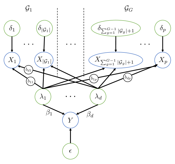
In some applications, the features naturally come partitioned into groups $\mathcal{G}_{1},\dots,\mathcal{G}_{G}$. Examples of such partitions are distinct functional networks of genes, features with significant versus features with non-significant association to the outcome in a previous study, and feature groups based on prior expert knowledge of feature importance (see, e.g., Münch et al., 2019). Figure 1 displays model (1) with partitioned features as a Bayesian network.

Figure 1: Model (1) with paritioned features as a Bayesian network, where the vertical dotted lines denote a partitioning of features $X_{1},\dots,X_{p}$ into groups $g=1,\dots,G$. Green and blue circles denote latent and observed variables, respectively. Note that the $\delta_{j}$ and $\epsilon$ are implicit in model (1) and omitted there for brevity. Here they denote the Gaussian, centred errors. That is, we have $y=\bm{\beta}^{\text{T}}\bm{\lambda}+\epsilon$, $\mathbf{x}=\mathbf{B}^{\text{T}}\bm{\lambda}+\bm{\delta}$, with $\epsilon\sim\mathcal{N}(0,\sigma^{2})$ and $\bm{\delta}\sim\mathcal{N}_{p}(0,\bm{\Psi})$.

Straightforward inclusion of the partitioning is possible through (i) a factor loadings partitioning, i.e., $\mathbf{B}=\begin{bmatrix}\begin{array}[]{c|c|c}\mathbf{B}_{1}&\cdots&\mathbf{B}_{G}\end{array}\end{bmatrix}$, or (ii) a uniquenessess partitioning, i.e.,

$$\bm{\Psi}=\begin{bmatrix}\bm{\Psi}_{1}&&\\ &\ddots&\\ &&\bm{\Psi}_{G}\end{bmatrix}.$$

Prediction (2) shows that the effect of inflation of diagonal element $\psi_{j}$ or shrinkage of column $\mathbf{b}_{j}$ on the induced regression coefficients $\tilde{\bm{\beta}}$ and $\bm{\beta}^{*}$, is similar. With an appropriate choice of priors for $\mathbf{B}$ and $\psi_{j},\dots,\psi_{p}$, the partitioning of the features $\mathcal{G}_{1},\dots,\mathcal{G}_{G}$ is included in the prior model. Here, We pursue option (i) and model the feature structure through the $\mathbf{B}$ prior, by considering groupwise constant (up to a uniquenessess scaling) prior variances, i.e., $\forall j\in\mathcal{G}_{g}:\gamma_{j}=\gamma_{g}$. The groupwise constant prior variance shrinks feature effects in the same group similarly. A small group-specific prior variance results in more shrinkage of feature effects, compared to a group with larger group-specific prior variance. By setting the group variances, the prior expected relevance of the group’s features is encoded in the model. However, determining the prior variances is not straighforward in most applications. Section 3.3 proposes an empirical Bayes approach to estimate these variances.

3 Estimation

Maximum likelihood estimation of model (3) is straightforward when $n<\bar{p}$ and many algorithms are available in literature. In the $\bar{p}>n$ domain, estimation is possible through penalized likelihood maximisation. In the current paper, focus is on the Bayesian model, so we refer the reader to Sections 9.1 and 9.2 of the SM for details on maximum (penalized) likelihood estimation of (3).

Bayesian posteriors are commonly approximated through MCMC sampling. Sampling from the posterior of model (3) and (5) is relatively straightforward (see SM Section 10.1 for a Gibbs sampler). However, due to high-dimensionality of the parameters, sampling is relatively slow. In addition, the MCMC chain shows poor mixing in all investigated applications and simulations. Poorly mixing MCMC chains require a prohibitive number of samples to properly explore the posterior. Here, we avoid computationally expensive MCMC sampling by a mean-field variational Bayes approximation of the posterior.

Mean-field variational Bayes methods minimise the Kullback-Leibler divergence of the posterior from the (approximate) variational posterior. With observed variables $\mathbf{X}$, some partitioning of unobserved variables $\bm{\theta}=\{\theta_{1},\dots,\theta_{K}\}$, and an factorised posterior assumption $p(\bm{\theta}|\mathbf{X})\approx\prod_{k=1}^{K}q(\theta_{k})$, this results in marginal posteriors $q(\theta_{k})\propto\exp\{\mathbb{E}_{\bm{\theta}_{-k}|\theta_{k},\mathbf{X}}\left[\log p(\theta_{k}|\bm{\theta}_{-k},\mathbf{X})\right]\}$. Note that we slightly abuse notation and let $q(\cdot)$ denote distinct densities based on the corresponding argument. For $p(\theta_{k}|\bm{\theta}_{-k},\mathbf{X})$ in the exponential family, $q(\theta_{k})$ is in the same exponential family with natural parameter $\mathbb{E}_{\bm{\theta}_{-k}|\theta_{k},\mathbf{X}}\left[\eta(\bm{\theta}_{-k},\mathbf{X})\right]$, where $\eta(\bm{\theta}_{-k},\mathbf{X})$ is the natural parameter of the full conditional distribution Blei et al. (2017).

Here, let $\bm{\Lambda}=\begin{bmatrix}\bm{\lambda}_{1}&\cdots\bm{\lambda}_{n}\end{bmatrix}^{\text{T}}$ and the approximate posterior factorise as

$$p(\bm{\Lambda},\bar{\mathbf{B}},\bar{\psi}_{1},\dots,\bar{\psi}_{\bar{p}}|\bar{\mathbf{X}})\approx q(\bm{\Lambda})q(\bar{\mathbf{B}})q(\bar{\psi}_{1},\dots,\bar{\psi}_{\bar{p}}),$$ (7)

so that the approximate posterior that minimises the Kullback-Leibler divergence of posterior to approximation is

$$q(\bm{\Lambda}) \overset{D}{=}\prod_{i=1}^{n}\mathcal{N}_{d}(\bm{\phi}_{i},\bm{\Xi}),$$ (8a)

$$q(\bar{\mathbf{B}}) \overset{D}{=}\prod_{\bar{j}=1}^{\bar{p}}\mathcal{N}_{d}(\bm{\mu}_{\bar{j}},\bm{\Omega}_{\bar{j}}),$$ (8b)

$$q(\bar{\psi}_{1},\dots,\bar{\psi}_{\bar{p}}) \overset{D}{=}\prod_{\bar{j}=1}^{\bar{p}}\Gamma^{-1}(n/2+d/2+\kappa_{\bar{j}},\zeta_{\bar{j}}).$$ (8c)

The so-called variational parameters are

$$\bm{\phi}_{i} =\left\{\sum_{{\bar{j}}=1}^{\bar{p}}\mathbb{E}(\bar{\psi}_{\bar{j}}^{-1})\left[\mathbb{V}(\bar{\mathbf{b}}_{\bar{j}})+\mathbb{E}(\bar{\mathbf{b}}_{\bar{j}})\mathbb{E}(\bar{\mathbf{b}}^{\text{T}}_{\bar{j}})\right]+\mathbf{I}_{d}\right\}^{-1}\mathbb{E}(\bar{\mathbf{B}})\mathbb{E}(\bar{\bm{\Psi}}^{-1})\bar{\mathbf{x}}_{i},\,i=1,\dots,n,$$ (9a)

$$\bm{\Xi} =\left\{\sum_{{\bar{j}}=1}^{\bar{p}}\mathbb{E}(\bar{\psi}_{\bar{j}}^{-1})\left[\mathbb{V}(\bar{\mathbf{b}}_{\bar{j}})+\mathbb{E}(\bar{\mathbf{b}}_{\bar{j}})\mathbb{E}(\bar{\mathbf{b}}_{\bar{j}}^{\text{T}})\right]+\mathbf{I}_{d}\right\}^{-1},$$ (9b)

$$\bm{\mu}_{\bar{j}} =\left[\mathbb{E}(\bm{\Lambda}^{\text{T}})\mathbb{E}(\bm{\Lambda})+n\mathbb{V}(\mathbf{\bm{\lambda}}_{i})+\gamma_{{\bar{j}}}^{-1}\mathbf{I}_{d}\right]^{-1}\mathbb{E}(\bm{\Lambda}^{\text{T}})\bar{\mathbf{x}}_{\bar{j}},\,{\bar{j}}=1,\dots,\bar{p},$$ (9c)

$$\bm{\Omega}_{\bar{j}} =\mathbb{E}(\psi_{\bar{j}}^{-1})^{-1}\left[\mathbb{E}(\bm{\Lambda}^{\text{T}})\mathbb{E}(\bm{\Lambda})+n\mathbb{V}(\mathbf{\bm{\lambda}}_{i})+\gamma_{{\bar{j}}}^{-1}\mathbf{I}_{d}\right]^{-1},\,{\bar{j}}=1,\dots\bar{p},$$ (9d)

$$\zeta_{\bar{j}} =\bar{\mathbf{x}}_{\bar{j}}^{\text{T}}\bar{\mathbf{x}}_{\bar{j}}/2-\mathbb{E}(\bar{\mathbf{b}}_{\bar{j}}^{\text{T}})\mathbb{E}(\bm{\Lambda}^{\text{T}})\bar{\mathbf{x}}_{\bar{j}}+\text{tr}\left[\mathbb{E}(\bm{\Lambda}^{\text{T}})\mathbb{E}(\bm{\Lambda})\mathbb{V}(\bar{\mathbf{b}}_{\bar{j}})\right]/2+n\text{tr}\left[\mathbb{V}(\bm{\lambda}_{i})\mathbb{V}(\bar{\mathbf{b}}_{\bar{j}})\right]/2$$

$$\,\,\,\,\,\,\,\,\,+\mathbb{E}(\bar{\mathbf{b}}_{\bar{j}}^{\text{T}})\mathbb{E}(\bm{\Lambda}^{\text{T}})\mathbb{E}(\bm{\Lambda})\mathbb{E}(\bar{\mathbf{b}}_{\bar{j}})/2+n\mathbb{E}(\bar{\mathbf{b}}_{\bar{j}}^{\text{T}})\mathbb{V}(\bm{\lambda}_{i})\mathbb{E}(\bar{\mathbf{b}}_{\bar{j}})/2+\gamma_{\bar{j}}^{-1}\mathbb{E}(\mathbf{b}_{\bar{j}}^{\text{T}})\mathbb{E}(\mathbf{b}_{\bar{j}})/2$$ (9e)

$$\,\,\,\,\,\,\,\,\,+\gamma_{\bar{j}}^{-1}\text{tr}\left[\mathbb{V}(\mathbf{b}_{\bar{j}})\right]/2+\nu_{\bar{j}},\,{\bar{j}}=1,\dots,{\bar{p}},$$

where we slightly abuse notation and let $\bar{\mathbf{x}}_{i}$ and $\bar{\mathbf{x}}_{\bar{j}}$ denote the $i$th row and $\bar{j}$th column of $\bar{\mathbf{X}}$, respectively. The expectations and variances are

$$\mathbb{E}(\bar{\psi}_{\bar{j}}^{-1}) =(n/2+d/2+\kappa_{\bar{j}})/\zeta_{\bar{j}},\,{\bar{j}}=1,\dots,{\bar{p}},$$

$$\mathbb{E}(\bar{\mathbf{b}}_{\bar{j}}) =\bm{\mu}_{\bar{j}},\,{\bar{j}}=1,\dots,{\bar{p}},$$

$$\mathbb{V}(\bar{\mathbf{b}}_{\bar{j}}) =\bm{\Omega}_{\bar{j}},\,{\bar{j}}=1,\dots,{\bar{p}},$$

$$\mathbb{E}(\bm{\Lambda}) =\bm{\Phi},$$

$$\mathbb{V}(\bm{\lambda}_{i}) =\bm{\Xi},\,i=1,\dots,n,$$

with $\bm{\Phi}=\begin{bmatrix}\bm{\phi}_{1}&\cdots\bm{\phi}_{n}\end{bmatrix}^{\text{T}}$. The parameters contain cyclic dependencies and are updated until convergence.

Model (1) describes a general covariance matrix. However, a correlation matrix better describes the standardised data. In the frequentist setting the general covariance model is straightforward to extend to the correlation model by restriction of the likelihood to the space of correlation matrices. Moreover, this is the default setting in the R package factanal. In the Bayesian setting, this requires either more intricate prior modelling or post hoc corrections of the posterior. Here, we consider a post hoc correction that ensures that the posterior expectation of the covariance of $\bar{\mathbf{X}}$ desribes a correlation matrix:

$$\forall\bar{j}:\mathbb{E}_{\bar{\mathbf{B}},\bar{\psi}_{1},\dots,\bar{\psi}_{\bar{p}}|\bar{\mathbf{X}}}\left(\bar{\mathbf{b}}_{\bar{j}}^{\text{T}}\bar{\mathbf{b}}_{\bar{j}}+{\bar{\psi}}_{\bar{j}}\right)=1.$$

SM Section 10.4 contains more details on this posterior correction and a possible future direct correlation modelling approach. In the following, the post hoc correction approach is applied.

3.1 Unlabeled observations

Inspection of (2) learns that the predictions $\mathbb{E}(\tilde{y}|\tilde{\mathbf{x}})$ depend on the observational model for $\mathbf{x}$ through $\mathbf{B}$ and $\bm{\Psi}$. As detailed in Liang et al. (2007), this implies that estimation benefits from additional unlabeled features $\mathbf{x}_{i}$, $i=n+1,\dots,n+m$, with the corresponding unobserved outcomes $z_{i}$, $i=n+1,\dots n+m$. A straightforward method of including the unlabeled observations is to consider the full data likelihood $p(\mathbf{X},\mathbf{z},\mathbf{y}|\bar{\mathbf{B}},\bar{\bm{\Psi}})$, with $\mathbf{z}=\begin{bmatrix}z_{n+1}&\cdots&z_{n+m}\end{bmatrix}^{\text{T}}$ Bańbura and Modugno (2014); Liu and Rubin (1998). Maximum likelihood estimation then requires marginalisation over unobserved outcomes $z_{i}$. Section 9.3 in the SM describes an EM algorithm for (penalized) maximum likelihood estimation with missing data.

In the Bayesian model, the unobserved outcomes are now included in the posterior distributions. The variational Bayes posterior (7) is augmented as

$$p(\bm{\Lambda},\bar{\mathbf{B}},\bar{\psi}_{1},\dots,\bar{\psi}_{\bar{p}},\mathbf{z}|\bar{\mathbf{X}})\approx q(\bm{\Lambda})q(\bar{\mathbf{B}})q(\bar{\psi}_{1},\dots,\bar{\psi}_{\bar{p}})q(\mathbf{z}),$$

where

$$q(\mathbf{z}) \overset{D}{=}\prod_{i={n+1}}^{n+m}\mathcal{N}(\upsilon_{i},\chi)\text{, with}$$

$$\upsilon_{i} =\mathbb{E}(\bar{\mathbf{b}}_{\bar{p}}^{\text{T}})\mathbb{E}(\bm{\lambda}_{i}),$$

$$\chi =\mathbb{E}(\bar{\psi}_{\bar{p}}^{-1})^{-1}.$$

In addition, the term $\mathbbm{1}_{\bar{j}=\bar{p}}m\mathbb{V}(z_{i})/2$ is added to (9e) and all occurences of $\bar{\mathbf{x}}_{i}$ and $\bar{\mathbf{x}}_{\bar{j}}$ in (9) are replaced with $\tilde{\mathbf{x}}_{i}$ and $\tilde{\mathbf{x}}_{\bar{j}}$, where

$$\tilde{\mathbf{X}}=\begin{bmatrix}\lx@intercol\hfil\hbox{\multirowsetup$\mathbf{X}$}\hfil\lx@intercol&\mathbf{y}\\ \lx@intercol\hfil\hfil\lx@intercol&\mathbb{E}(\mathbf{z})\end{bmatrix},$$

and

$$\mathbb{E}(z_{i}) =\upsilon_{i},$$

$$\mathbb{V}(z_{i}) =\chi.$$

SM Section 10.1 contains more details on the inclusion of unlabeled observations in the (approximate) Bayesian posterior computations through MCMC. Although not shown here due to brevity, the unobserved outcome approach is straightforward to extend to an unobserved features approach.

3.2 Latent dimension

Although we initially assumed $d$ to be the true latent dimension, in general it is unkown and needs to be estimated. Methods for dimension estimation are plentiful in the literature (see, e.g., Zwick and Velicer, 1986). Our modest aim of accurate prediction does not require correct estimation of the latent dimension, as even picking the true latent dimension does not always lead to optimal predictions Goeman (2006). Without this requirement of correct latent dimension estimation, we resort to the simple and fast Kaiser criterion. The Kaiser criterion picks $d$ that retains dimensions with variance contribution larger than that of the average feature $\mathbf{x}$. This amounts to choosing $d=\sum_{j=1}^{p}\mathbbm{1}\{v_{j}>1\}$, with $v_{j}$, $j=1,\dots,p$, the eigenvalues of the correlation matrix. That is, we set $d$ to the number of eigenvalues of the correlation matrix of $\mathbf{X}$ larger than one.

3.3 Hyperparameters

The Bayesian model requires a choice of hyperparameters $\gamma_{g}$, $\kappa_{j}$ and $\nu_{j}$. Choosing the $\gamma_{g}$ by hand requires intricate prior expert knowledge, which might not be available. An alternative is to estimate them from the data using empirical Bayes. Or, if we do know the overall scale of the $\gamma_{g}$, but not the group-specific deviations, we may reparametrise as $\gamma_{g}=\gamma\gamma_{g}^{\prime}$, fix the overall scale $\gamma$ and estimate the group-specific multipliers $\gamma_{g}^{\prime}$.

In both empirical Bayes settings we maximise the marginal likelihood (constrained maximisation for the second approach). Direct marginal likelihood maximisation requires calculation of a $p$-dimensional integral for which no closed form is available. With $p$ large (i.e., the high dimensional setup considered here), an EM algorithm with iterations

$$\bm{\gamma}^{(k+1)}=\underset{\bm{\gamma}}{\text{argmax}\,}\mathbb{E}_{\theta|\mathbf{y}}\left[\log p(\bar{\mathbf{B}}|\bar{\psi}_{1},\dots,\bar{\psi}_{\bar{p}})|\bm{\gamma}^{(k)}\right],$$

where $\bm{\gamma}=\begin{bmatrix}\gamma_{1}&\cdots\gamma_{G}\end{bmatrix}^{\text{T}}$, is computationally much more feasible. With a variational Bayes approximation of the difficult expectation, this results in

$$\bm{\gamma}^{(k+1)}=\underset{\bm{\gamma}}{\text{argmax}\,}\left\{-\frac{1}{2}\sum_{g=1}^{G}\gamma_{g}^{-1}\sum_{j\in\mathcal{G}_{g}}\mathbb{E}(\bar{\psi}_{j}^{-1})\left\{\text{tr}\left[\mathbb{V}(\bar{\mathbf{b}}_{j})\right]+\mathbb{E}(\bar{\mathbf{b}}_{j}^{\text{T}})\mathbb{E}(\bar{\mathbf{b}}_{j})\right\}-\frac{d}{2}\sum_{g=1}^{G}|\mathcal{G}_{g}|\log\gamma_{g}\right\}.$$

Finally, this gives empirical Bayes updates:

$$\gamma_{g}^{(k+1)}=\frac{\sum_{j\in\mathcal{G}_{g}}\mathbb{E}(\bar{\psi}_{j}^{-1})\left\{\text{tr}\left[\mathbb{V}(\bar{\mathbf{b}}_{j})\right]+\mathbb{E}(\bar{\mathbf{b}}_{j}^{\text{T}})\mathbb{E}(\bar{\mathbf{b}}_{j})\right\}}{|\mathcal{G}_{g}|d}.$$

For the $\gamma_{g}=\gamma\gamma_{g}^{\prime}$ parametrisation, the updates

$$\bm{\gamma}^{\prime(k+1)} =\underset{\bm{\gamma}^{\prime}}{\text{argmax}\,}\left\{-\frac{1}{\gamma}\sum_{g=1}^{G}\gamma_{g}^{\prime-1}\sum_{j\in\mathcal{G}_{g}}\mathbb{E}(\bar{\psi}_{j}^{-1})\left\{\text{tr}\left[\mathbb{V}(\bar{\mathbf{b}}_{j})\right]+\mathbb{E}(\bar{\mathbf{b}}_{j}^{\text{T}})\mathbb{E}(\bar{\mathbf{b}}_{j})\right\}-\frac{d}{2}\sum_{g=1}^{G}|\mathcal{G}_{g}|\log\gamma_{g}^{\prime}\right\},$$

$$\text{subject to }\prod_{g=1}^{G}\gamma_{g}^{\prime|\mathcal{G}_{g}|}=1,$$

are not available in closed form, but still convex and easy to compute with standard numerical optimisation tools. Empirical Bayes estimation of the $\gamma_{g}$ or $\gamma_{g}^{\prime}$ is data-dependent and does not rely on subjective arguments. In addition, empirical Bayes estimation avoids (possibly complicated) hyperpriors on the $\gamma_{g}$ and $\gamma_{g}^{\prime}$. A drawback is that we lose the uncertainty propagation property of the full Bayesian approach.

Prior error variance/uniquenesses shapes $\kappa_{\bar{j}}$ and scale $\nu_{\bar{j}}$, and overall prior variance $\gamma$ are set to default values to reflect a lack of prior knowledge. Our default choice of hyperparameters should take the standardisation of the data into account. Three postulates are used to select the hyperparameters: (i) we ensure that the prior expectation describes a correlation matrix model, i.e., $\forall j:\mathbb{E}_{\bar{\mathbf{B}},\bar{\psi}_{1},\dots,\bar{\psi}_{\bar{p}}}(\bar{\mathbf{b}}_{\bar{j}}^{\text{T}}\bar{\mathbf{b}}_{\bar{j}}+{\bar{\psi}}_{\bar{j}})=1$. Furthermore, (ii) the prior contributions of the error and the latent structure to the data are assumed equal, i.e., $\forall j:\mathbb{E}_{\bar{\mathbf{B}},\bar{\psi}_{1},\dots,\bar{\psi}_{\bar{p}}}(\bar{\mathbf{b}}_{\bar{j}}^{\text{T}}\bar{\mathbf{b}}_{\bar{j}})=\mathbb{E}_{\bar{\mathbf{B}},\bar{\psi}_{1},\dots,\bar{\psi}_{\bar{p}}}({\bar{\psi}}_{\bar{j}})=1/2$. Lastly, (iii) the prior uniqueness variance is set to $\mathbb{V}_{\bar{\mathbf{B}},\bar{\psi}_{1},\dots,\bar{\psi}_{\bar{p}}}({\bar{\psi}}_{\bar{j}})=1$. These three postulates together result in $\gamma=1/d$, $\forall\bar{j}:\kappa_{\bar{j}}=9$, and $\forall\bar{j}:\nu_{\bar{j}}=4$. As a result, $\forall{\bar{j}}:\mathbb{V}_{\bar{\mathbf{B}},\bar{\psi}_{1},\dots,\bar{\psi}_{\bar{p}}}(\mathbf{b}_{j}^{\text{T}}\mathbf{b}_{j})=1+5/(2d)$. For $d$ large compared to $5/2$ (as one expects in high-dimensional settings), we have $\mathbb{V}_{\bar{\mathbf{B}},\bar{\psi}_{1},\dots,\bar{\psi}_{\bar{p}}}(\mathbf{b}_{j}^{\text{T}}\mathbf{b}_{j})\approx 1=\mathbb{V}_{\bar{\mathbf{B}},\bar{\psi}_{1},\dots,\bar{\psi}_{\bar{p}}}({\bar{\psi}}_{\bar{j}})$, so that the contributions to the prior variance of latent structure and error are approximately equal. The methods described in this Section are implemented in the R package bayesfactanal available from https://github.com/magnusmunch/bayesfactanal.

4 Simulations

To assess the potential benefit of the proposed models in prediction of outcome $y$ from features $\mathbf{x}$, a simulation is set up. The simulation setting is meant to demonstrate the potential benefit of (i) the Bayesian factor regression model in general, (ii) the inclusion of the feature structure through the empirical Bayes estimation of the $\gamma_{g}^{\prime}$ as explained in Section 3.3, and (iii) the use of unlabeled features in the estimation.

To that end, $n=50$ labeled, and $m\in\{0,50,100,200,500\}$ unlabeled observations are drawn from model (1) and standardised after simulation. Error variance and uniquenesses are set to $\sigma^{2}=1$ and $\forall j:\psi_{j}=1$. The number of features is fixed to $p=100$. Two scenarios for the model parameters $b_{hj}$ and $\beta_{h}$ are considered:

1. the number of factors are fixed to $d=10$. The $b_{hj}$ are set so that each feature loads on two factors and factor is a part of 20 features (see (10), where each $b$ denotes 10 values and the empty cells are set to zero). $\beta_{h}$ is set so that the outcome loads on all factors. The features are divided in two groups $\mathcal{G}_{1}=\{1,\dots,50\}$ and $\mathcal{G}_{2}=\{51,\dots,100\}$. The non-zero $b_{hj}$ are drawn from independent univariate centered Gaussian distributions. The variances are $\mathbb{V}(b_{hj})=0.1$ for $j=1,\dots 50$, and $\mathbb{V}(b_{hj})=1$ for $j=51,\dots,100$ The $\beta_{h}$ are independent and drawn from the standard Gaussian distribution.

2. The second scenario fixes $d=40$. The model parameters $b_{hj}$ are drawn from independent univariate centered Gaussian distributions. The variances are $\mathbb{V}(b_{hj})=0.1$ for $j=1,\dots 50$, and $\mathbb{V}(b_{hj})=10$ for $j=51,\dots,100$, i.e., the features are structured in two groups: $\mathcal{G}_{1}=\{1,\dots,50\}$ and $\mathcal{G}_{2}=\{51,\dots,100\}$. To ensure that the proportion of variance in $y$ explained with the factors is 0.7, $\beta_{h}$ is set $\beta_{h}=0.483$.

$$\mathbf{B}=\left[\begin{array}[]{ c c c c c:c c c c c}b&&&&&&&&&b\\ b&b&&&&&&&&\\ &b&b&&&&&&&\\ &&b&b&&&&&&\\ &&&b&b&&&&&\\ &&&&b&b&&&&\\ &&&&&b&b&&&\\ &&&&&&b&b&&\\ &&&&&&&b&b&\\ &&&&&&&&b&b\end{array}\right]$$ (10)

The first scenario models a situation where the features load on two factors only in such a way that the marginal correlation between features is weak. This might occur, for example, if genes are organised in nearly disjoint functional networks, but the outcome is related to all the networks. Ridge regression is expected to perform well here. With such a sparse loadings matrix, $(\mathbf{B}^{\text{T}}\mathbf{B}+\bm{\Psi})^{-1}\approx\mathbf{I}_{p}$. That is, the information in $\mathbf{X}$ contributes little to the induced regression coefficients $\tilde{\bm{\beta}}$. In addition, the induced regression coefficients become $\tilde{\bm{\beta}}\approx\mathbf{B}^{\text{T}}\bm{\beta}=\mathbb{C}\text{ov}(y,\mathbf{x})$, a (rescaled version of the) quantity that standard linear regression methods aim to estimate.

The second scenario models a setting where all features load on all factors, but the strength of the loading depends on the feature group. This might occur, for example, if genes are organised in several interconnected functional networks, but some network have weak connections. The outcome is again related to the all functional networks. In this setting, the factor regression methods are expected to perform well. In contrast to the first simulation, $(\mathbf{B}^{\text{T}}\mathbf{B}+\bm{\Psi})^{-1}\neq\mathbf{I}_{p}$, so information on the induced regression coefficients $\tilde{\bm{\beta}}$ is contained in $\mathbf{X}$. This results in increased effiency due to the inclusion of data. Also, $\tilde{\bm{\beta}}$, is a weighted version of $\mathbb{C}\text{ov}(y,\mathbf{x})$ that is not straightforward to estimate with standard linear regression methods.

Six models are compared:

1. Ridge regression with cross validated penalty parameter with the R package glmnet Friedman et al. (2010);

2. Lasso regression with cross validated penalty parameter with the R glmnet package Friedman et al. (2010);

3. a two-step factor regression method: (i) a penalized factor model is estimated from the feature correlation matrix, with cross validated penalty parameter. Next, (ii) outcomes are regressed on the feature factor scores $\hat{\mathbb{E}}(\bm{\lambda}_{i}|\mathbf{x}_{i})$ to obtain the prediction rule. This approach was shown to work in Peeters et al. (2019a) and is implemented in the R FMradio package Peeters et al. (2019b);

4. a penalized factor regression model that includes unlabeled observations, with cross validated penalty parameter, and estimated as in SM Section (9);

5. the proposed Bayesian factor regression model (5), approximated with variational Bayes as in Section 3. The fixed hyperparameters are described in Section 3.3. Note that this model does not include external feature structure and therefore does not estimate the $\gamma_{g}^{\prime}$;

6. the proposed empirical Bayesian factor regression model (5), approximated with variational Bayes as in Section 3. The hyperparameters are described in Section 3.3, where we include the grouping of the features and estimate group-specific $\gamma_{g}^{\prime}$ by empirical Bayes.

For all models, the data are standardised before estimation, as is common in most real data applications. Models 3-6 allow for the inclusion of unlabeled features and are estimated for a range of number of unlabeled features. In addition, we fitted an intercept-only null model. We calculate estimation mean squared error (EMSE) of $\tilde{\bm{\beta}}$, prediction mean squared error (PMSE), and correlation between predictions and observations ($\mathbb{C}\text{or}(y,\hat{y})$) on test data of size $n_{\text{test}}=1000$. Lower PMSE and EMSE indicate better performance, while higher $\mathbb{C}\text{or}(y,\hat{y})$ indicates better performance. The results, with the median taken over 50 simulation replications, are displayed in Figures 2 and Figures 3, for scenarios 1 and 2, respectively.

Figure 2: Simulation results for scenario 1 with median (a) EMSE and (b) PMSE, respectively.

Figure 3: Simulation results for scenario 2 with median (a) EMSE and (b) PMSE, respectively.

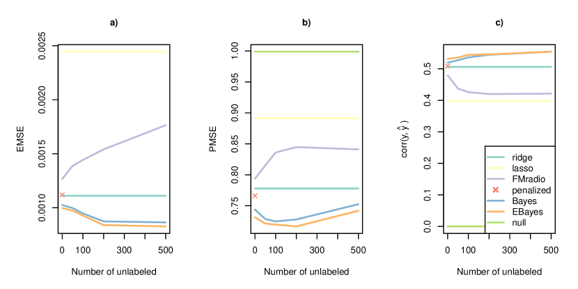
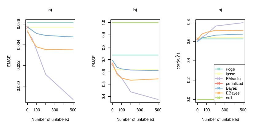
In both scenarios, the penalized factor regression model was not estimable with unlabeled data, due to non-convergence. The two-step FMradio approach also suffers from non-convergence with more unlabeled data, but was still estimable in some simulations, so it is included in the Figures.

In both scenarios estimation (i.e., EMSE) and prediction calibration (i.e., PMSE) of the Bayesian methods initially improves with more unlabeled data. However, in scenario 1 it starts deteriorating again after about $m=100$. Surprisingly, the opposite holds for FMradio. In scenario 2, where the performance continues to improve with more unlabeled data, the rate of improvement decreases with the number of unlabeled observations. This is unsurprising, as estimators generally converge at a similarly-shaped $\sqrt{n}$ rate. In both scenarios, discrimination (i.e., $\mathbb{C}\text{or}(y,\hat{y})$) keeps improving with the addition of unlabeled features. For scenario 1, this is surprising, considering the eventual deterioration in calibration and estimation.

In scenario 1, the Bayesian methods outperform the frequentist methods for almost all $m$ in terms of estimation and discrimination. Calibration is worse for the Bayesian methods for small and large $m$, but better for medium $m$. The two-step factor regression model FMradio, performs worse than the Bayesian factor regression methods and ridge, only outperforming lasso. In scenario 2, the frequentist methods outperform the Bayesian method for small $m$ in terms of estimation and calibration. For medium $m$, the Bayesian methods outperform ridge, and eventally, for large $m$, also lasso. FMradio outperforms all other methods in estimation, calibration, and discrimination. Scenario 2 simulates strong factors, that explain much of the data. Extraction of these factors in step one of the FMradio approach is therefore relatively easy. Estimation of the prediction rule based on these strong factors in step two of FMradio then results in a strong predictor.

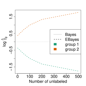
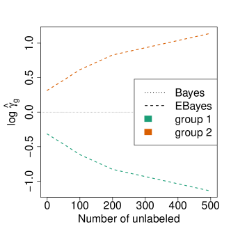
A comparison of full Bayes and empirical Bayes shows that the inclusion of the feature groupings helps in both estimation and prediction. In scenario 1, empirical Bayes estimation and calibration is slightly better than full Bayes. Discrimination is about equal. In scenario 2 empirical clearly outperforms full Bayes in all three performance measures. Figures 4 and 5 display the estimated $\log\hat{\gamma}^{\prime}_{g}$ for the empirical Bayes model in scenarios 1 and 2, respectively. Both Figures show a clear influence of the feature grouping on estimation, as the prior variances of the groups show a clear difference. Furthermore, the influence of the feature grouping grows with the number of unlabeled observations, as the diverging lines indicate.

Figure 4: Simulation results for scenario 1 with median $\log\hat{\gamma}_{g}^{\prime}$ estimated with empirical Bayes.

Figure 5: Simulation results for scenario 2 with median $\log\hat{\gamma}_{g}^{\prime}$ estimated with empirical Bayes.

5 Applications

5.1 Influenza vaccine

The data described in this Section are from Nakaya et al. (2011) and made publicly available through the NCBI GEO archive Barrett et al. (2012) with accession numbers GSE29614 and GSE29617. The analysis mostly follows Van Deun et al. (2018), where a main aim was to predict vaccine efficacy with microarray gene expression data. Here follows a short description of the data; for more details we refer the reader to Van Deun et al. (2018).

The data are from 9 and 26 subjects, observed in the 2007 and 2008 flu seasons, respectively. For all subjects there are three efficacy measures from just before and 28 after vaccination available in the form of three different plasma hemagglutination inhibition (HAI) antibody titers. The antibody titers were combined by first taking the maximum of the three log-transformed titers and then substracting the measurements just before and three days after vaccination. The scores were standardised to mean zero and variance one. In addition to the vaccine efficacy measures, there are 54,675 microarray gene expression measurements available from just before and three days after vaccination. The Robust Multichip Average (RMA) algorithm Irizarry (2003) was used to pre-process the microarrays. After pre-processing, a change score was calculated by substracting the measurements just before and three days after vaccination from each other. These scores were standardised to mean zero and variance one. Before the analysis, a pre-selection of 416 genes with highest coefficient of variation is made. The choice of 416 genes follows the analysis results of Van Deun et al. (2018). Here, we consider the 2007 data as unlabeled and the 2008 data as labeled.

The application is an example of a difficult high-dimensional prediction problem, with little data available: a situation that regularly arises in practice. Here, the available unlabeled data potentially increases predictive performance signficicantly. Additionally, genes are often considered to be organised in functional networks, so the factor model is an appropriate choice and we expect the factor regression methods to outperform classical linear regression methods.

We estimate the same models as in Section 4, with the exception of the empirical Bayes model, because there is no grouping of the features available. To assess performance we calculated cross-validated PMSE and $\mathbb{C}\text{or}(y,\hat{y})$ and display them in Table 1, where null refers to the intercept only model. The penalized factor regression model did not converge, so is not included in the results.

Table 1: Cross-validated PMSE and $\mathbb{C}\text{or}(y,\hat{y})$ (best performing in bold) calculated on the influenza vaccine data.

	PMSE	$\mathbb{C}\text{or}(y,\hat{y})$
ridge	0.959	0.171
lasso	0.929	0.339
FMradio	0.955	0.097
VBayes	0.866	0.341
null	0.962	0

Table 1 shows that the variational Bayesian factor regression that includes the unlabeled data outperforms the other methods in terms of calibration (i.e., PMSE) and discrimination (i.e., $\mathbb{C}\text{or}(y,\hat{y})$), according to expectation. The other methods perform similarly in terms of PMSE, while lasso performance approaches the Bayesian factor regression in terms of $\mathbb{C}\text{or}(y,\hat{y})$.

5.2 Oral cancer lymph node metastasis

In this Section, oral cancer lymph node metastasis is predicted with gene expression data. RNAseqs, taken from TCGA The Cancer Genome Atlas Network (2015), are measured on 133 HPV-negative oral tumours taken from 76 and 57 oral cancer patients, with and without lymph node metastasis, respectively. For more details on these data, see te Beest et al. (2017). Additional gene expressions are available from an independent microarray study on 97 oral cancer patients in Mes et al. (2017). These microarrays are normalised to the same scale as the RNAseqs and included in the analysis as unlabeled data. A set of 871 genes with $p\leq 0.01$ in the microarray data is pre-selected. To investigate the empirical Bayes estimation of the $\gamma_{g}$, the genes are divided in three groups, based on the cis-correlation between between the RNAseq data and TCGA DNA copy numbers on the same patients, quantified by Kendall’s $\tau$.

This Section investigates an example of a high-dimensional classification problem in for which both unlabeled data and external feature information is available. As before, genes are assumed to be organised in functional networks, so we expect the factor regression methods to fit the data well. We expect features with a large positive correlation between RNAseqs and DNA copy number, as quantified by Kendall’s $\tau$, to be more important for metastasis prediction. We therefore expect to estimate larger $\gamma_{g}^{\prime}$ for the groups with higher Kendall’s $\tau$.

We estimate the logistic extensions of the models estimated in Section 4. To assess performance we calculated a calibration measure Brier skill score (BSS) and discrimination measure area under the receiver operator curve (AUC) on the unlabeled data and display them in Table 2. The penalized factor regression model did not converge, so is not included in the results.

Table 2: BSS and AUC (best performing in bold) calculated on the oral cancer lymph node metastasis data.

	BSS	AUC
ridge	0.125	0.698
lasso	0.132	0.708
FMradio	0.014	0.66
VBayes	0.099	0.746
EBayes	0.101	0.748

Surprisingly, the best performing model in terms of calibration (i.e., BSS) is the lasso. The Bayesian factor regression methods outperform the other methods in terms of discrimination (i.e., AUC). The estimated $\gamma_{g}^{\prime}$ are $0.97$, $0.98$, and $1.01$ for the low-, medium-, and high cis-correlation groups, respectively. This small difference in shrinkage leads to a marginal increase in predictive performance of the empirical Bayes method compared to the full Bayes version.

6 Discussion

This paper investigates a Bayesian factor regression model for high dimensional prediction and classification problems. It allows for the inclusion of unlabeled data and feature groupings to improve predictive performance. Estimation is through a combination of variational and empirical Bayes techniques. The approach is competitive with classical ridge and lasso regression, as well as with more elaborate frequentist factor modelling approaches such as penalized factor regression and the two-step factor FMradio. Simulations show that the method is especially useful if the features are generated in dense, correlated networks. Two applications show that the method predicts just as well, or better, than existing methods in real data settings.

A technical advantage of the pursued factor modelling approach is the straightforward inclusion of unlabeled observations through the full likelihood approach. However, some caution regarding this approach is advised. For the full likelihood approach to return unbiased estimates, the missing data mechanism is assumed to be at most missing at random (MAR). That is, the missingness possibly depends on the observed features, but not on unobserved features. In the current setting, MAR implies that unobserved labels are not missing due to the value of the labels. We argue that in most applications, this is a reasonable assumption. In the examples above, observations are unlabeled because they come from independent studies. Due to the independence, it is reasonable to assume that no relation exists between not observing labels and the actual labels. Another technical advantage of Bayesian modelling is the occurence of convergence issues in frequentist models. Sections 4 and 5 show that the frequentist factor models suffer from convergence issues if the number of labeled and/or unlabeled samples becomes large. More investigation is required to determine when and why these convergence issues occur. An inherent benefit of Bayesian modelling is the uncertainty quantification that automatically comes with the Bayesian posterior. This allows for straightforward calculation of prediction intervals. We note that the uncertainty quantification in the current setting requires a more thorough investigation.

More elaborate prior modelling of the factor loadings is possible through the $\gamma_{j}$. For example, a more sparse lasso model for the factor loadings introduces the hyperpriors: $\gamma_{j}\sim\text{Exp}(\lambda_{j})$. Feature grouping is then included by parametrising $\forall j\in\mathcal{G}_{g}:\lambda_{j}=\lambda_{g}$, and estimating the $\lambda_{g}$ with empirical Bayes. In general, such Gaussian scale mixture extensions of the $\bar{\mathbf{B}}$ prior require the addition of one or more extra layers to the prior and one or more extra variational parameters to update during estimation. Some existing examples of sparse Bayesian factor models are Ferrari and Dunson (2020) and Carvalho et al. (2008). Sparse factor models often simplify the latent dimension estimation. In any case, latent dimension estimation is a topic that deserves more attention. Here, estimation is via a simple Kaiser criterion. More elaborate methods are available in literature (see, e.g., Auerswald and Moshagen, 2019).

Lastly, we give some indication of computational times. The proposed factor regression approaches are slower to estimate compared to the other methods. Model estimation times for the influenza application are: 0.87, 0.16, 5.27, and 36.46 seconds, for the ridge, lasso, FMradio, and Bayesian factor regression models, respectively. For the oral cancer metastasis appication we have 2.76, 0.98 and 54.82 seconds for the ridge, lasso and FMradio, and 124.68 and 245.18 minutes for the variational and empirical Bayesian models. Especially in the second application, the estimation is considerably slower. However, we argue that these times are still manageable and much faster than traditional MCMC estimation times.

Supplementary Material to: ‘Semi-supervised empirical Bayes group-regularized factor regression’

7 Introduction

This document contains Supplementary Material (SM) to the Main Document (MD) titled ‘Semi-supervised empirical Bayes group-regularized factor regression’.

8 Model identifiability and determinancy

Two issues arise from MD model (3): (i) Rotational unidentifiability and (ii) indeterminancy in the latent factors. Issue (i) becomes apparent if we multiply the loadings with an orthogonal matrix $\mathbf{H}$ and consider the implied covariance matrix:

$$\mathbb{C}\text{ov}(\bar{\mathbf{x}})=\bar{\mathbf{B}}^{\text{T}}\bar{\mathbf{B}}+\bar{\bm{\Psi}}=(\mathbf{H}\bar{\mathbf{B}})^{\text{T}}(\mathbf{H}\bar{\mathbf{B}})+\bar{\bm{\Psi}}.$$ (11)

From (11) we see that any arbitrary orthogonal transformation yields the same covariance. This indeterminancy is usually fixed by restricting $\bar{\mathbf{B}}\bar{\bm{\Psi}}^{-1}\bar{\mathbf{B}}^{\text{T}}$ to a diagonal matrix during maximum likelihood estimation. This restriction has no apparent interpretation, so to increase the interpretability of the model, a post hoc rotation of the loadings is often desirable. A popular choice is the orthogonal Varimax rotation, which maximises the sum of the variances of the squared loadings. Varimax rotation often leads to approximately sparse representations of features that benefit interpretability.

Issue (ii), indeterminancy of latent factors, stems from the initial postulate $\mathbb{E}(\bm{\lambda}\bm{\lambda}^{\text{T}})=\mathbf{I}_{d}$. The predicted scores $\hat{\bm{\lambda}}=\mathbb{E}(\bm{\lambda}|\bar{\mathbf{x}})$ do not necessarily adhere to this postulate:

$$\mathbb{E}(\hat{\bm{\lambda}}\hat{\bm{\lambda}}^{\text{T}})=\bar{\mathbf{B}}(\bar{\mathbf{B}}^{\text{T}}\bar{\mathbf{B}}+\bar{\bm{\Psi}})^{-1}\bar{\mathbf{B}}^{\text{T}}\neq\mathbf{I}_{d}.$$

However, we can generate a random variable $\mathbf{s}$, uncorrelated to $\bar{\mathbf{x}}$, and with expectation $\mathbf{0}_{d}$ and variance $\mathbf{I}_{d}$ to construct scores:

$$\hat{\bm{\lambda}}=\bar{\mathbf{B}}(\bar{\mathbf{B}}^{\text{T}}\bar{\mathbf{B}}+\bar{\bm{\Psi}})^{-1}\bar{\mathbf{B}}^{\text{T}}+\left[\mathbf{I}_{d}-\bar{\mathbf{B}}(\bar{\mathbf{B}}^{\text{T}}\bar{\mathbf{B}}+\bar{\bm{\Psi}})^{-1}\bar{\mathbf{B}}^{\text{T}}\right]^{1/2}\mathbf{s},$$

that do adhere to the postulate. Unfortunately, there are infinitely many choices of $\mathbf{s}$, leading to an indeterminancy in the latent factors. A simple fix to this indeterminancy is setting $\bar{\bm{\Psi}}=n^{-1}[(\bar{\mathbf{X}}^{\text{T}}\bar{\mathbf{X}})^{-1}\circ\mathbf{I}_{p}]^{-1}$.

9 Maximum likelihood estimation

9.1 Maximum likelihood

In the low-dimensional setting ($\bar{p}<n$), loadings $\bar{\mathbf{B}}$ and variances $\bar{\psi}_{1},\dots,\bar{\psi}_{\bar{p}}$ in MD model (3) may be estimated by maximum likelihood. If we denote the parameters by $\theta=\{\bar{\mathbf{B}},\bar{\psi}_{1},\dots,\bar{\psi}_{\bar{p}}\}$, the maximum likelihood estimate is given by Mardia (1979):

$$\hat{\theta}=\underset{\theta}{\text{argmax}\,}\log|\bar{\bm{\Sigma}}^{-1}|-\text{tr}\left(\bar{\bm{\Sigma}}^{-1}\bar{\mathbf{S}}\right),$$ (12)

where $\bar{\bm{\Sigma}}=\bar{\mathbf{B}}^{\text{T}}\bar{\mathbf{B}}+\bar{\bm{\Psi}}$, and $\bar{\mathbf{S}}=n^{-1}\bar{\mathbf{X}}^{\text{T}}\bar{\mathbf{X}}$ is the empirical covariance matrix of $\bar{\mathbf{X}}$. The maximum likelihood estimation is implemented in the base R package stats as the factanal function.

9.2 Penalised maximum likelihood

In high dimensional settings, i.e., $\bar{p}>n$, the unique (up to rotation) maximum likelihood estimate of MD model (3) does not exist. One solution is to penalise the likelihood van Wieringen and Peeters (2016):

$$\hat{\theta}=\underset{\theta}{\text{argmax}\,}\log|\bar{\bm{\Sigma}}^{-1}|-(1-\gamma)\text{tr}\left(\bar{\bm{\Sigma}}^{-1}\bar{\mathbf{S}}\right)-\gamma\text{tr}\left(\bar{\bm{\Sigma}}^{-1}\bm{\Gamma}\right),$$ (13)

where $\gamma\in\left(0,1\right]$ is a penalty parameter that determines the amount of penalisation and $\bm{\Gamma}$ is a positive definite shrinkage target matrix, usually taken to be diagonal, or even the identity. Computing (13) is easily done via factanal in R, where the empirical covariance is replaced with its shrunken estimate $(1-\gamma)\bar{\mathbf{S}}+\gamma\bm{\Gamma}$. Common choices for target $\bm{\Gamma}$ are van Wieringen and Peeters (2016) $\bm{\Gamma}=\mathbf{I}_{p}$ and $\bm{\Gamma}$ diagonal with $\bm{\Gamma}_{jj}=\bar{\mathbf{S}}_{jj}$. A convenient and data-drive method to pick penalty parameter $\gamma$ is $k$-fold cross validation, as described in Peeters et al. (2019a).

The attentive reader may have noticed that the penalty in (13) is not a proper penalty. The added penalty term is $\gamma\text{tr}[\bar{\bm{\Sigma}}^{-1}(\bm{\Gamma}-\bar{\mathbf{S}})]$, which does not necessarily penalise the likelihood if $\bm{\Gamma}-\bar{\mathbf{S}}>0$ somewhere. It is however, a “penalty” with good empirical performance. In addition, it automatically models a correlation matrix if both the empirical covariance and shrinkage targets are proper correlation matrices.

9.3 Unlabeled features

To incorporate the observed, unlabeled features $\mathbf{x}_{i}$, for $i=n+1,\dots,n+m$, we treat the unobserved, corresponding responses $z_{i}$, for $i=n+1,\dots,n+m$, as missing and employ an EM algorithm to incorporate them into the likelihood maximisation. Writing $\mathbf{z}=\begin{bmatrix}z_{n+1}&\cdots&z_{n+m}\end{bmatrix}^{\text{T}}$ for the unobserved responses and $\theta^{(k)}=\{\bar{\mathbf{B}}^{(k)},\bar{\psi}_{1}^{(k)},\dots,\bar{\psi}_{\bar{p}}^{(k)}\}$ for the current parameter estimates, we have respective E- and M-steps:

$$Q(\theta|\theta^{(k)}) =\mathbb{E}_{\mathbf{z}|\mathbf{y},\mathbf{X}}\left[\log p\left(\mathbf{z},\mathbf{y},\mathbf{X}\right)|\theta^{(k)}\right],$$ (14a)

$$\theta^{(k+1)} =\underset{\theta}{\text{argmax}\,}Q(\theta|\theta^{(k)}),$$ (14b)

which we iteratively apply until convergence of the expected log likelihood (14a).

The E-step in (14a) is:

$$\mathbb{E}_{\mathbf{z}|\mathbf{y},\mathbf{X}}\left[\log p\left(\mathbf{z},\mathbf{y},\mathbf{X}\right)|\theta^{(k)}\right]\propto\sum_{i=1}^{n}\log p(y_{i},\mathbf{x}_{i}|\theta^{(k)})+\sum_{i=n+1}^{n+m}\mathbb{E}_{z_{i}|\mathbf{x}_{i}}\left[\log p(z_{i},\mathbf{x}_{i}|\theta^{(k)})\right].$$

The first term is just the regular likelihood that is maximised in (12). The second term may be written as:

$$\sum_{i=n+1}^{n+m}\mathbb{E}_{z_{i}|\mathbf{x}_{i}}\left[\log p(z_{i},\mathbf{x}_{i}|\theta^{(k)})\right] \propto\log|\bar{\bm{\Sigma}}|-m^{-1}\sum_{i=n+1}^{n+m}\mathbb{E}_{z_{i}|\mathbf{x}_{i}}\left(\begin{bmatrix}\mathbf{x}_{i}^{\text{T}}&z_{i}\end{bmatrix}\bar{\bm{\Sigma}}^{-1}\begin{bmatrix}\mathbf{x}_{i}^{\text{T}}&z_{i}\end{bmatrix}^{\text{T}}\right)$$

$$=\log|\bar{\bm{\Sigma}}|-\text{tr}\left[\bar{\bm{\Sigma}}^{-1}m^{-1}\sum_{i=n+1}^{n+m}\mathbb{E}_{z_{i}|\mathbf{x}_{i}}\left(\begin{bmatrix}\mathbf{x}_{i}^{\text{T}}&z_{i}\end{bmatrix}^{\text{T}}\begin{bmatrix}\mathbf{x}_{i}^{\text{T}}&z_{i}\end{bmatrix}\right)\right]$$

$$=\log|\bar{\bm{\Sigma}}|-\text{tr}\left(\bar{\bm{\Sigma}}^{-1}\tilde{\mathbf{S}}_{-n}\right),$$

where we have written:

$$\tilde{\mathbf{S}}_{-n} =m^{-1}\sum_{i=n+1}^{n+m}\mathbb{E}_{z_{i}|\mathbf{x}_{i}}\left(\begin{bmatrix}\mathbf{x}_{i}^{\text{T}}&z_{i}\end{bmatrix}^{\text{T}}\begin{bmatrix}\mathbf{x}_{i}^{\text{T}}&z_{i}\end{bmatrix}\right)$$

$$=m^{-1}\sum_{i=n+1}^{n+m}\left[\mathbb{E}_{z_{i}|\mathbf{x}_{i}}\left(\begin{bmatrix}\mathbf{x}_{i}^{\text{T}}&z_{i}\end{bmatrix}^{\text{T}}\right)\mathbb{E}_{z_{i}|\mathbf{x}_{i}}\left(\begin{bmatrix}\mathbf{x}_{i}^{\text{T}}&z_{i}\end{bmatrix}\right)+\mathbb{V}_{z_{i}|\mathbf{x}_{i}}\left(\begin{bmatrix}\mathbf{x}_{i}^{\text{T}}&z_{i}\end{bmatrix}^{\text{T}}\right)\right]$$

$$=m^{-1}\left(\tilde{\mathbf{X}}_{-n}^{\text{T}}\tilde{\mathbf{X}}_{-n}+\begin{bmatrix}\mathbf{0}_{p\times p}&\mathbf{0}_{p\times 1}\\ \mathbf{0}_{1\times p}&m\mathbb{V}_{z|\mathbf{x}}(z|\theta^{(k)})\end{bmatrix}\right),$$

with

$$\tilde{\mathbf{X}}_{-n}^{\text{T}}=\begin{bmatrix}\mathbf{x}_{n+1}^{\text{T}}&\mathbb{E}_{z_{n+1}|\mathbf{x}_{n+1}}(z_{n+1}|\theta^{(k)})\\ \vdots&\vdots\\ \mathbf{x}_{n+m}^{\text{T}}&\mathbb{E}_{z_{n+m}|\mathbf{x}_{n+m}}(z_{n+m}|\theta^{(k)})\\ \end{bmatrix}.$$ (16)

Now if we combine this term with the regular likelihood term we have:

$$\mathbb{E}_{\mathbf{z}|\mathbf{y},\mathbf{X}}\left[\log p\left(\mathbf{z},\mathbf{y},\mathbf{X}\right)|\theta^{(k)}\right]\propto\log|\bar{\bm{\Sigma}}^{-1}|-\text{tr}\left(\bar{\bm{\Sigma}}^{-1}\tilde{\mathbf{S}}\right),$$ (17)

where

$$\tilde{\mathbf{S}}=(n+m)^{-1}\left(\tilde{\mathbf{X}}^{\text{T}}\tilde{\mathbf{X}}+\begin{bmatrix}\mathbf{0}_{p\times p}&\mathbf{0}_{p\times 1}\\ \mathbf{0}_{1\times p}&m\mathbb{V}_{z|\mathbf{x}}(z|\theta^{(k)})\end{bmatrix}\right),$$ (18)

and

$$\tilde{\mathbf{X}}=\begin{bmatrix}\bar{\mathbf{X}}\\ \tilde{\mathbf{X}}_{-n}\end{bmatrix}.$$ (19)

The expectations and variance in (16) and (18) are easily derived from the well-known relation between the joint multivariate normal distribution in (3) and the corresponding conditional distributions:

$$\mathbb{E}_{z_{i}|\mathbf{x}_{i}}(z_{i}|\theta^{(k)}) =\mathbf{x}_{i}^{\text{T}}\left[(\mathbf{B}^{(k)})^{\text{T}}\mathbf{B}^{(k)}+\bm{\Psi}^{(k)}\right]^{-1}(\mathbf{B}^{(k)})^{\text{T}}\bm{\beta}^{(k)},$$

$$\mathbb{V}_{z|\mathbf{x}}(z|\theta^{(k)}) =(\bm{\beta}^{(k)})^{\text{T}}\left\{\mathbf{I}_{d}-\mathbf{B}^{(k)}\left[(\mathbf{B}^{(k)})^{\text{T}}\mathbf{B}^{(k)}+\bm{\Psi}^{(k)}\right]^{-1}(\mathbf{B}^{(k)})^{\text{T}}\right\}\bm{\beta}^{(k)}+(\sigma^{2})^{(k)}.$$

The M-step in (17) is easily computed as before in (12), using the factanal function in R with the augmented empirical covariance $\tilde{\mathbf{S}}$ instead of $\bar{\mathbf{S}}$. The above is easily generalised to include data with arbitrary missingness patterns.

10 Bayesian inference

In this Section it is useful to note that the likelihood MD (3) of i.i.d. Gaussian data $\bar{\mathbf{X}}=\begin{bmatrix}\bar{\mathbf{x}}_{1}&\cdots&\bar{\mathbf{x}}_{n}\end{bmatrix}^{\text{T}}$ may be rewritten as a product over densities of columns $\bar{\mathbf{x}}_{\bar{j}}$, $\bar{j}=1,\dots,\bar{p}$, instead of the observations $\bar{\mathbf{x}}_{i}$, $i=1,\dots,n$, where we abuse notation to indicate column (and thus variable) $\bar{j}$ of $\bar{\mathbf{X}}$ by $\bar{\mathbf{x}}_{\bar{j}}$ and row (and thus observation) $i$ by $\bar{\mathbf{x}}_{i}$:

$$\prod_{i=1}^{n}p(\bar{\mathbf{x}}_{i}|\bm{\lambda}_{i},\bar{\mathbf{B}},\bar{\psi}_{1},\dots,\bar{\psi}_{\bar{p}})=\prod_{\bar{j}=1}^{\bar{p}}p(\bar{\mathbf{x}}_{\bar{j}}|\bm{\Lambda},\bar{\mathbf{b}}_{\bar{j}},\bar{\psi}_{\bar{j}}),$$ (21)

with $\bm{\Lambda}=\begin{bmatrix}\bm{\lambda}_{1}&\cdots&\bm{\lambda}_{n}\end{bmatrix}^{\text{T}}$ and

$$p(\bar{\mathbf{x}}_{\bar{j}}|\bm{\Lambda},\bar{\mathbf{b}}_{\bar{j}},\bar{\psi}_{\bar{j}})\overset{D}{=}\mathcal{N}_{n}\left(\bm{\Lambda}\bar{\mathbf{b}}_{\bar{j}},\psi_{\bar{j}}\mathbf{I}_{n}\right).$$

10.1 Gibbs sampling

This Section derives the full conditionals of the Bayesian model in (3) and (5). To that end, in this Section, we include the unlabeled features and unobserved outcomes into $\bar{\mathbf{X}}$, i.e.,

$$\bar{\mathbf{X}}_{(n+m)\times\bar{p}}=\begin{bmatrix}\lx@intercol\hfil\hbox{\multirowsetup$\mathbf{X}$}\hfil\lx@intercol&\mathbf{y}\\ \lx@intercol\hfil\hfil\lx@intercol&\mathbf{z}\end{bmatrix}.$$

In addition, we slightly abuse notation, write $\bar{\mathbf{x}}_{i}$ and $\bar{\mathbf{x}}_{j}$ as the $i$th row and $j$th column of $\bar{\mathbf{X}}$, respectively. Then, the full conditional for $\bm{\Lambda}$ is:

$$p(\bm{\Lambda}|\bar{\mathbf{X}},\bar{\mathbf{B}},\bar{\psi}_{1},\dots\bar{\psi}_{\bar{p}}) \propto\prod_{i=1}^{n+m}p(\bar{\mathbf{x}}_{i}|\bm{\lambda}_{i},\bar{\mathbf{B}},\bar{\psi}_{1},\dots\bar{\psi}_{\bar{p}})\prod_{i=1}^{n+m}p(\bm{\lambda}_{i})$$

$$\propto\prod_{i=1}^{n+m}\exp\left[-\frac{1}{2}(\bar{\mathbf{x}}_{i}-\bar{\mathbf{B}}^{\text{T}}\bm{\lambda}_{i})^{\text{T}}\bar{\bm{\Psi}}^{-1}(\bar{\mathbf{x}}_{i}-\bar{\mathbf{B}}^{\text{T}}\bm{\lambda}_{i})-\frac{1}{2}\bm{\lambda}_{i}^{\text{T}}\bm{\lambda}_{i}\right]$$

$$\propto\prod_{i=1}^{n+m}\exp\bigg{\{}-\frac{1}{2}\left[\bm{\lambda}_{i}-(\bar{\mathbf{B}}\bar{\bm{\Psi}}^{-1}\bar{\mathbf{B}}^{\text{T}}+\mathbf{I}_{d})^{-1}\bar{\mathbf{B}}\bar{\bm{\Psi}}^{-1}\bar{\mathbf{x}}_{i}\right]^{\text{T}}$$

$$\quad\quad\quad(\bar{\mathbf{B}}\bar{\bm{\Psi}}^{-1}\bar{\mathbf{B}}^{\text{T}}+\mathbf{I}_{d})\left[\bm{\lambda}_{i}-(\bar{\mathbf{B}}\bar{\bm{\Psi}}^{-1}\bar{\mathbf{B}}^{\text{T}}+\mathbf{I}_{d})^{-1}\bar{\mathbf{B}}\bar{\bm{\Psi}}^{-1}\bar{\mathbf{x}}_{i}\right]\bigg{\}},$$

which allows us to write:

$$\bm{\Lambda}|\bar{\mathbf{X}},\bar{\mathbf{B}},\bar{\psi}_{1},\dots\bar{\psi}_{\bar{p}} \sim\prod_{i=1}^{n+m}\mathcal{N}_{d}\left((\bar{\mathbf{B}}\bar{\bm{\Psi}}^{-1}\bar{\mathbf{B}}^{\text{T}}+\mathbf{I}_{d})^{-1}\bar{\mathbf{B}}\bar{\bm{\Psi}}^{-1}\bar{\mathbf{x}}_{i},(\bar{\mathbf{B}}\bar{\bm{\Psi}}^{-1}\bar{\mathbf{B}}^{\text{T}}+\mathbf{I}_{d})^{-1}\right).$$ (22)

Next, we consider

$$p(\bar{\mathbf{B}}|\bar{\mathbf{X}},\bm{\Lambda},\bar{\psi}_{1},\dots\bar{\psi}_{\bar{p}}) \propto\prod_{i=1}^{n+m}p(\bar{\mathbf{x}}_{i}|\bm{\lambda}_{i},\bar{\mathbf{B}},\bar{\psi}_{1},\dots\bar{\psi}_{\bar{p}})\prod_{\bar{j}=1}^{\bar{p}}p(\bar{\mathbf{b}}_{\bar{j}}|\bar{\psi}_{\bar{j}})$$

$$=\prod_{\bar{j}=1}^{\bar{p}}p(\bar{\mathbf{x}}_{\bar{j}}|\bm{\Lambda},\bar{\mathbf{b}}_{\bar{j}},\bar{\psi}_{\bar{j}})p(\bar{\mathbf{b}}_{\bar{j}}|\bar{\psi}_{\bar{j}})$$

$$\propto\prod_{\bar{j}=1}^{\bar{p}}\exp\left[\frac{\bar{\psi}_{\bar{j}}^{-1}}{2}(\bar{\mathbf{x}}_{\bar{j}}-\bm{\Lambda}\bar{\mathbf{b}}_{\bar{j}})^{\text{T}}(\bar{\mathbf{x}}_{\bar{j}}-\bm{\Lambda}\bar{\mathbf{b}}_{\bar{j}})-\frac{\gamma_{\bar{j}}^{-1}\bar{\psi}_{\bar{j}}^{-1}}{2}\bar{\mathbf{b}}_{\bar{j}}^{\text{T}}\bar{\mathbf{b}}_{\bar{j}}\right]$$

$$\propto\prod_{\bar{j}=1}^{\bar{p}}\exp\bigg{\{}-\frac{1}{2}\left[\bar{\mathbf{b}}_{\bar{j}}-(\bm{\Lambda}^{\text{T}}\bm{\Lambda}+\gamma^{-1}_{\bar{j}}\mathbf{I}_{d})^{-1}\bm{\Lambda}^{\text{T}}\bar{\mathbf{x}}_{\bar{j}}\right]^{\text{T}}$$

$$\quad\quad\quad\bar{\psi}_{\bar{j}}^{-1}(\bm{\Lambda}^{\text{T}}\bm{\Lambda}+\gamma^{-1}_{\bar{j}}\mathbf{I}_{d})\left[\bar{\mathbf{b}}_{\bar{j}}-(\bm{\Lambda}^{\text{T}}\bm{\Lambda}+\gamma^{-1}_{\bar{j}}\mathbf{I}_{d})^{-1}\bm{\Lambda}^{\text{T}}\bar{\mathbf{x}}_{\bar{j}}\right]\bigg{\}},$$

which gives

$$\bar{\mathbf{B}}|\bar{\mathbf{X}},\bm{\Lambda},\bar{\psi}_{1},\dots\bar{\psi}_{\bar{p}}\sim\prod_{\bar{j}=1}^{\bar{p}}\mathcal{N}_{d}\left((\bm{\Lambda}^{\text{T}}\bm{\Lambda}+\gamma^{-1}_{\bar{j}}\mathbf{I}_{d})^{-1}\bm{\Lambda}^{\text{T}}\bar{\mathbf{x}}_{\bar{j}},\bar{\psi}_{\bar{j}}(\bm{\Lambda}^{\text{T}}\bm{\Lambda}+\gamma^{-1}_{\bar{j}}\mathbf{I}_{d})^{-1}\right).$$ (23)

For the $\bar{\psi}_{\bar{j}}$, we derive:

$$p(\bar{\psi}_{1},\dots\bar{\psi}_{\bar{p}}|\bar{\mathbf{X}},\bm{\Lambda},\bar{\mathbf{B}}) \propto\prod_{i=1}^{n+m}p(\bar{\mathbf{x}}_{i}|\bm{\lambda}_{i},\bar{\mathbf{B}},\bar{\psi}_{1},\dots\bar{\psi}_{\bar{p}})\prod_{\bar{j}=1}^{\bar{p}}p(\bar{\mathbf{b}}_{\bar{j}}|\bar{\psi}_{\bar{j}})p(\bar{\psi}_{\bar{j}})$$

$$=\prod_{\bar{j}=1}^{\bar{p}}p(\bar{\mathbf{x}}_{\bar{j}}|\bm{\Lambda},\bar{\mathbf{b}}_{\bar{j}},\bar{\psi}_{\bar{j}})p(\bar{\mathbf{b}}_{\bar{j}}|\bar{\psi}_{\bar{j}})p(\bar{\psi}_{\bar{j}})$$

$$\propto\prod_{\bar{j}=1}^{\bar{p}}\bar{\psi}_{\bar{j}}^{-(\frac{n+m+d}{2}+\kappa_{\bar{j}})-1}$$

$$\quad\quad\quad\exp\left\{-\bar{\psi}_{\bar{j}}^{-1}\left[\frac{1}{2}(\bar{\mathbf{x}}_{\bar{j}}-\bm{\Lambda}\bar{\mathbf{b}}_{\bar{j}})^{\text{T}}(\bar{\mathbf{x}}_{\bar{j}}-\bm{\Lambda}\bar{\mathbf{b}}_{\bar{j}})+\frac{\gamma^{-1}_{\bar{j}}}{2}\bar{\mathbf{b}}_{\bar{j}}^{\text{T}}\bar{\mathbf{b}}_{\bar{j}}+\nu_{\bar{j}}\right]\right\},$$

to arrive at

$$\bar{\psi}_{1},\dots\bar{\psi}_{\bar{p}}|\bar{\mathbf{X}},\bm{\Lambda},\bar{\mathbf{B}}\sim\prod_{\bar{j}=1}^{\bar{p}}\Gamma^{-1}\left(\frac{n+m+d}{2}+\kappa_{\bar{j}},\frac{1}{2}(\bar{\mathbf{x}}_{\bar{j}}-\bm{\Lambda}\bar{\mathbf{b}}_{\bar{j}})^{\text{T}}(\bar{\mathbf{x}}_{\bar{j}}-\bm{\Lambda}\bar{\mathbf{b}}_{\bar{j}})+\frac{\gamma_{\bar{j}}^{-1}}{2}\bar{\mathbf{b}}_{\bar{j}}^{\text{T}}\bar{\mathbf{b}}_{\bar{j}}+\nu_{j}\right).$$ (24)

Given the latent variables and parameters, $z$ is independent of $\mathbf{x}$, so the full conditional for the missing outcomes is equal to the likelihood:

$$\mathbf{z}|\mathbf{X},\bm{\Lambda},\bar{\mathbf{B}},\bar{\psi}_{1},\dots\bar{\psi}_{\bar{p}}\sim\prod_{i=n+1}^{n+m}\mathcal{N}(\bar{\mathbf{b}}_{\bar{p}}^{\text{T}}\bm{\lambda}_{i},\bar{\psi}_{\bar{p}}).$$ (25)

Using these full conditionals, samples from the posterior may be generated through a straightforward Gibbs sampling scheme.

10.2 Variational evidence lower bound

Variational parameters are generally updated until convergence of the evidence lower bound. Here we describe a general case of our evidence lower bound, in which missingness may be occur in all all variables (i.e., both response and features). The number of missing values for feature $\bar{j}$ is indicated with $m_{\bar{j}}$. Let $\tau_{\bar{j}}=(n/2+d/2+\kappa_{\bar{j}})/(2\zeta_{\bar{j}})$, then:

$$\text{ELBO}= -\frac{np-\sum_{{\bar{j}}=1}^{\bar{p}}m_{\bar{j}}}{2}\log 2\pi+\frac{nd+pn+dp+\sum_{{\bar{j}}=1}^{\bar{p}}m_{\bar{j}}}{2}$$

$$+\sum_{{\bar{j}}=1}^{{\bar{p}}}\left[\log\Gamma\left(\frac{n+d}{2}+\kappa_{\bar{j}}\right)-\log\Gamma(\kappa_{\bar{j}})-\frac{d}{2}\psi\left(\frac{n+d}{2}+\kappa_{\bar{j}}\right)+\frac{d}{2}\log\gamma_{\bar{j}}+\kappa_{\bar{j}}\left(1+\log\nu_{\bar{j}}\right)\right]$$

$$+\sum_{{\bar{j}}=1}^{{\bar{p}}}\left[\frac{m_{\bar{j}}}{2}\log\chi_{\bar{j}}-\tau_{\bar{j}}m_{\bar{j}}\chi_{\bar{j}}-\left(\frac{n-d}{2}+\kappa_{\bar{j}}\right)\log\zeta_{\bar{j}}-\frac{1}{2}\nu_{\bar{j}}\tau_{\bar{j}}\right]$$

$$+\sum_{{\bar{j}}=1}^{\bar{p}}\left[\frac{1}{2}\log|\bm{\Omega}_{\bar{j}}|-\tau_{\bar{j}}\gamma_{\bar{j}}^{-1}\text{tr}\left(\bm{\Omega}_{\bar{j}}\right)-n\tau_{\bar{j}}\text{tr}\left(\bm{\Xi}\bm{\Omega}_{\bar{j}}\right)-\tau_{\bar{j}}\text{tr}\left(\bm{\Phi}^{\text{T}}\bm{\Phi}\bm{\Omega}_{\bar{j}}\right)\right]$$

$$+2\text{tr}\left[\text{diag}\left(\tau_{\bar{j}}\right)\tilde{\mathbf{X}}^{\text{T}}\bm{\Phi}\mathbf{M}\right]-n\text{tr}\left[\text{diag}\left(\tau_{\bar{j}}\right)\mathbf{M}^{\text{T}}\bm{\Xi}\mathbf{M}\right]-\text{tr}\left[\text{diag}\left(\tau_{j}\gamma_{\bar{j}}^{-1}\right)\mathbf{M}^{\text{T}}\mathbf{M}\right]$$

$$-\text{tr}\left[\text{diag}\left(\tau_{\bar{j}}\right)\mathbf{M}^{\text{T}}\bm{\Phi}^{\text{T}}\bm{\Phi}\mathbf{M}\right]-\text{tr}\left[\text{diag}\left(\tau_{\bar{j}}\right)\tilde{\mathbf{X}}^{\text{T}}\tilde{\mathbf{X}}\right]$$

$$+\frac{n}{2}\log|\bm{\Xi}|-\frac{n}{2}\text{tr}(\bm{\Xi})-\frac{1}{2}\text{tr}\left(\bm{\Phi}^{\text{T}}\bm{\Phi}\right),$$

where $\psi(x)$ denotes the digamma function and $\mathbf{M}=\begin{bmatrix}\bm{\mu}_{1}&\cdots&\bm{\mu}_{{\bar{p}}}\end{bmatrix}$.

10.3 Posterior expectation

In the (variational) Bayesian model, the prediction rule $\mathbb{E}(\tilde{y}|\tilde{\mathbf{x}})$ is not available in closed-form. In the MD, we approximate it with Monte Carlo simulations from the posterior. This is generally fast, because it requires sample from multivariate Gaussian and inverse Gamma distributions, for which fast sampling algorithms are available.

Alternatively, one may approximate the expectation with a truncated Taylor series. If we denote $\theta=\{\mathbf{B},\bm{\beta},\bm{\psi}_{1},\dots,\psi_{p}\}$ and $g(\theta)=\tilde{\mathbf{x}}^{\text{T}}(\mathbf{B}^{\text{T}}\mathbf{B}+\bm{\Psi})^{-1}\mathbf{B}^{\text{T}}\bm{\beta}$, a second order Taylor approximation around the variational posterior mean of the parameters is:

$$\mathbb{E}(\tilde{y}|\tilde{\mathbf{x}}) =\mathbb{E}\left[g(\theta)\right]$$

$$\approx g\left[\mathbb{E}(\theta)\right]+\frac{1}{2}\text{tr}\left[\frac{\partial^{2}g(\theta)}{\partial\theta^{2}}\bigg{|}_{\theta=\mathbb{E}(\theta)}\mathbb{V}(\theta)\right].$$

The mean-field assumption and form of the variational posterior allow us to write:

$$\mathbb{E}(\tilde{y}|\tilde{\mathbf{x}}) \approx g\left[\mathbb{E}(\theta)\right]+\frac{1}{2}\sum_{j=1}^{p}\text{tr}\left[\frac{\partial^{2}g(\theta)}{\partial\mathbf{b}_{j}\partial\mathbf{b}_{j}^{\text{T}}}\bigg{|}_{\mathbf{b}_{j}=\mathbb{E}(\mathbf{b}_{j})}\mathbb{V}(\mathbf{b}_{j})\right]+\frac{1}{2}\sum_{j=1}^{p}\left[\frac{\partial^{2}g(\theta)}{\partial\psi_{j}^{2}}\bigg{|}_{\psi_{j}=\mathbb{E}(\psi_{j})}\mathbb{V}(\psi_{j})\right],$$ (26)

where we have used that

$$\frac{\partial^{2}g(\theta)}{\partial\bm{\beta}\partial\bm{\beta}^{\text{T}}}=\mathbf{0}.$$

The derivative in the third term of the right-hand side of (26) is given by:

$$\frac{\partial^{2}g(\theta)}{\partial\psi_{j}^{2}}=2\tilde{\mathbf{x}}^{\text{T}}[(\mathbf{B}^{\text{T}}\mathbf{B}+\bm{\Psi})^{-1}]_{jj}[(\mathbf{B}^{\text{T}}\mathbf{B}+\bm{\Psi})^{-1}]_{j}^{\text{T}}[(\mathbf{B}^{\text{T}}\mathbf{B}+\bm{\Psi})^{-1}]_{j}\mathbf{B}^{\text{T}}\bm{\beta},$$

so that we can write:

$$\frac{1}{2}\sum_{j=1}^{p}\left[\frac{\partial^{2}g(\theta)}{\partial\psi_{j}^{2}}\bigg{|}_{\psi_{j}=\mathbb{E}(\psi_{j})}\mathbb{V}(\psi_{j})\right]=\tilde{\mathbf{x}}^{\text{T}}\mathbf{B}^{\text{T}}\bm{\beta}\text{tr}\left\{\text{diag}\left[(\mathbf{B}^{\text{T}}\mathbf{B}+\bm{\Psi})^{-1}\right](\mathbf{B}^{\text{T}}\mathbf{B}+\bm{\Psi})^{-2}\text{diag}[\mathbb{V}(\psi_{j})]\right\}.$$

The trace involving the derivatives with respect to $\mathbf{b}_{j}$ in the second term in the right-hand side (26) is a bit more involved. We write $\mathbf{E}=(\mathbf{B}^{\text{T}}\mathbf{B}+\bm{\Psi})^{-1}$ and only retain the non-zero parts when deriving with respect to $\mathbf{b}_{j}$:

$$\partial^{2}g(\theta)=2\tilde{\mathbf{x}}^{\text{T}}\Big{[} \mathbf{E}(\partial\mathbf{B})^{\text{T}}\mathbf{B}\mathbf{E}(\partial\mathbf{B})^{\text{T}}\mathbf{B}\mathbf{E}\mathbf{B}^{\text{T}}+2\mathbf{E}\mathbf{B}^{\text{T}}(\partial\mathbf{B})\mathbf{E}(\partial\mathbf{B})^{\text{T}}\mathbf{B}\mathbf{E}\mathbf{B}^{\text{T}}$$

$$+ 2\mathbf{E}(\partial\mathbf{B})^{\text{T}}\mathbf{B}\mathbf{E}\mathbf{B}^{\text{T}}(\partial\mathbf{B})\mathbf{E}\mathbf{B}^{\text{T}}+2\mathbf{E}\mathbf{B}^{\text{T}}(\partial\mathbf{B})\mathbf{E}\mathbf{B}^{\text{T}}(\partial\mathbf{B})\mathbf{E}\mathbf{B}^{\text{T}}$$

$$- 2\mathbf{E}(\partial\mathbf{B})^{\text{T}}(\partial\mathbf{B})\mathbf{E}\mathbf{B}^{\text{T}}-2\mathbf{E}(\partial\mathbf{B})^{\text{T}}\mathbf{B}\mathbf{E}(\partial\mathbf{B})^{\text{T}}-2\mathbf{E}\mathbf{B}^{\text{T}}(\partial\mathbf{B})\mathbf{E}(\partial\mathbf{B})^{\text{T}}\Big{]}\bm{\beta}.$$

Straightforward derivation of$\mathbf{B}$ with respect to $\mathbf{b}_{j}$ then gives a very messy expression, which we do not show here. Plugging into (26), together with $g[\mathbb{E}(\theta)]=\tilde{\mathbf{x}}^{\text{T}}(\mathbf{B}^{\text{T}}\mathbf{B}+\bm{\Psi})^{-1}\mathbf{B}^{\text{T}}\bm{\beta}|_{\theta=\mathbb{E}(\theta)}$, results in a fast approximation method for $\mathbb{E}(\tilde{y}|\tilde{\mathbf{x}})$ that is linear in $\tilde{\mathbf{x}}$.

10.4 Bayesian inference for correlation matrix

This Section considers two approaches to modelling a correlation matrix instead of a general covariance matrix.

10.4.1 Proper correlation modelling

We observe $n$ observations on $p$ standardised variables $\mathbf{x}$, i.e., $\sum_{i=1}^{n}x_{ij}=0,n^{-1}\sum_{i=1}^{n}x^{2}_{ij}=1$, $j=1,\dots,p$. The standardisation implies that we should model the correlation matrix instead of the covariance matrix. Write $\bm{\Psi}=\text{diag}(\psi_{j})$, for the diagonal matrix with unique variances $\psi_{j}$, $j=1,\dots,p$ on the diagonal, $\mathbf{B}_{d\times p}$ for the matrix of factor loadings, $\lambda$ for a vector of $d$ latent variables and consider the observational factor model:

$$\mathbf{x}|\bm{\lambda},\mathbf{B},\psi_{1},\dots,\psi_{p}, \sim\mathcal{N}_{p}\left(\mathbf{B}^{\text{T}}\bm{\lambda},\bm{\Psi}\right),$$ (27a)

$$\bm{\lambda} \sim\mathcal{N}_{d}\left(\mathbf{0}_{d\times 1},\mathbf{I}_{d}\right).$$ (27b)

Model (27) induces a marginal covariance matrix:

$$\mathbb{V}(\mathbf{x})=\mathbf{B}^{\text{T}}\mathbf{B}+\bm{\Psi},$$

which is a non-degenerate correlation matrix if we require $\forall j:\psi_{j}=1-\mathbf{b}_{j}^{\text{T}}\mathbf{b}_{j}>0$.

We now consider the Bayesian prior

$$\mathbf{B},\psi_{1},\dots,\psi_{p} \sim\prod_{j=1}^{p}\mathcal{N}_{d}(\mathbf{0}_{d\times 1},\gamma_{j}\mathbf{I}_{d})\mathbbm{1}\{\mathbf{b}_{j}^{\text{T}}\mathbf{b}_{j}<1\}\delta\left(\psi_{j}-1+\mathbf{b}_{j}^{\text{T}}\mathbf{b}_{j}\right).$$ (28)

This prior is a product of priors over variables $j=1,\dots,p$, with each variable $j$ prior itself a product of a multivariate normal for $\mathbf{b}_{j}$, truncated to a unit ball and a (degenerate) Dirac distribution for $\psi_{j}$. Introduction of the latent variables $\psi_{j}$ results in tractable (approximate) posterior computations, as will become clear later on. To see that prior (28) results in a model for a correlation matrix, we use (21) to integrate the joint distribution of data and prior over the $\psi_{j}$:

$$\int_{\psi_{1}}\cdots\int_{\psi_{p}} \prod_{i=1}^{n}p(\mathbf{x}_{i}|\bm{\lambda}_{i},\mathbf{B},\psi_{1},\dots,\psi_{p})p(\mathbf{B},\psi_{1},\dots,\psi_{j})d\psi_{1}\cdots d\psi_{j}$$

$$=\prod_{j=1}^{p}\int_{\psi_{j}}p(\mathbf{x}_{j}|\bm{\Lambda},\mathbf{b}_{j},\psi_{j})p(\mathbf{b}_{j},\psi_{j})d\psi_{j}=\prod_{j=1}^{p}p(\mathbf{x}_{j}|\bm{\Lambda},\mathbf{b}_{j})p(\mathbf{b}_{j})$$

$$=\prod_{i=1}^{n}p(\mathbf{x}_{i}|\bm{\lambda}_{i},\mathbf{B})p(\mathbf{B}),$$

where $p(\mathbf{x}_{i}|\bm{\lambda}_{i},\mathbf{B})$ corresponds to the observational model (27) with $\forall j:\psi_{j}=1-\mathbf{b}_{j}^{\text{T}}\mathbf{b}_{j}$ and the prior

$$p(\mathbf{B})\overset{D}{=}\prod_{j=1}^{p}\mathcal{N}_{d}(\mathbf{0}_{d\times 1},\gamma_{j}\mathbf{I}_{d})\mathbbm{1}\{\mathbf{b}_{j}^{\text{T}}\mathbf{b}_{j}<1\}$$

is truncated to the unit ball to ensure a non-degenerate correlation matrix.

A mean-field approximation to the posterior of model (27) and (28) is

$$p(\bm{\Lambda},\mathbf{B},\psi_{1},\dots,\psi_{p}|\mathbf{X})\approx q(\bm{\Lambda})q(\mathbf{B})q(\psi_{1},\dots,\psi_{p}),$$

such that the Kullback-Leibler divergence of the posterior from the (approximate) variational posterior is minimised. Here, a slight abuse of notation allows $q$ to refer to different functions depending on the input variable. In general, in mean-field variational Bayes with parameters $\bm{\theta}=\{\theta_{1},\dots,\theta_{K}\}$, data $\mathbf{X}$, and an assumed factorised approximate posterior: $p(\bm{\theta}|\mathbf{X})\approx\prod_{k=1}^{K}q(\theta_{k}|\mathbf{X})$, results in $q(\theta_{k}|\mathbf{X})\propto\exp\{\mathbb{E}_{\bm{\theta}_{-k}|\theta_{k},\mathbf{X}}\left[\log p(\theta_{k}|\bm{\theta}_{-k},\mathbf{X})\right]\}$. For model (27) and (28) this results in:

$$q(\bm{\Lambda}) \overset{D}{=}\prod_{i=1}^{n}\mathcal{N}_{d}(\bm{\phi}_{i},\bm{\Xi}),$$

$$q(\mathbf{B}) \overset{D}{=}\prod_{j=1}^{p}\mathcal{N}_{d}(\bm{\mu}^{*}_{j},\bm{\Omega}^{*}_{j})\mathbbm{1}\{\mathbf{b}_{j}^{\text{T}}\mathbf{b}_{j}<1\},$$

$$q(\psi_{1},\dots,\psi_{p}) \overset{D}{=}\prod_{j=1}^{p}\delta\left(\psi_{j}-\zeta_{j}\right),$$

with

$$\bm{\phi}_{i} =\left\{\sum_{j=1}^{p}\mathbb{E}(\psi_{j})^{-1}\left[\mathbb{V}(\bar{\mathbf{b}}_{j})+\mathbb{E}(\bar{\mathbf{b}}_{j})\mathbb{E}(\bar{\mathbf{b}}^{\text{T}}_{j})\right]+\mathbf{I}_{d}\right\}^{-1}\mathbb{E}(\bar{\mathbf{B}})\mathbb{E}(\bar{\bm{\Psi}})^{-1}\mathbf{x}_{i},$$

$$\bm{\Xi} =\left\{\sum_{j=1}^{p}\mathbb{E}(\psi_{j})^{-1}\left[\mathbb{V}(\bar{\mathbf{b}}_{j})+\mathbb{E}(\bar{\mathbf{b}}_{j})\mathbb{E}(\bar{\mathbf{b}}_{j}^{\text{T}})\right]+\mathbf{I}_{d}\right\}^{-1},$$

$$\bm{\mu}^{*}_{j} =\left[\mathbb{E}(\bm{\Lambda}^{\text{T}}\bm{\Lambda})+\gamma_{j}^{-1}\mathbf{I}_{d}\right]^{-1}\mathbb{E}(\bm{\Lambda}^{\text{T}})\mathbf{x}_{j},$$

$$\bm{\Omega}^{*}_{j} =\mathbb{E}(\psi_{j})\left[\mathbb{E}(\bm{\Lambda}^{\text{T}}\bm{\Lambda})+\gamma_{j}^{-1}\mathbf{I}_{d}\right]^{-1},$$

$$\zeta_{j} =1-\mathbb{E}(\bar{\mathbf{b}}_{j}^{\text{T}})\mathbb{E}(\bar{\mathbf{b}}_{j})-\text{tr}[\mathbb{V}(\bar{\mathbf{b}}_{j})].$$

The expectations involving $\bm{\Lambda}$ and $\psi_{j}$ are:

$$\mathbb{E}(\bm{\Lambda}^{\text{T}}\bm{\Lambda}) =n\bm{\Xi}+\bm{\Phi}^{\text{T}}\bm{\Phi},$$

$$\mathbb{E}(\bm{\Lambda}) =\bm{\Phi},$$

$$\mathbb{E}(\psi_{j}) =\zeta_{j}.$$

10.4.2 Elliptical truncated multivariate Gaussian

The expectations and variances involving the $\mathbf{b}_{j}$ are not available in closed form and little bit more involved. They are expectations and variances of multivariate elliptical truncated Gaussians. We resort to calculation using the moment generating function as in Arismendi and Broda (2017). This results in the following expressions for the expectation and variance:

$$\bm{\mu}_{j}=\mathbb{E}(\bar{\mathbf{b}}_{j}) =\bm{\mu}^{*}_{j}+L^{-1}\mathbf{v},$$

$$\bm{\Omega}_{j}=\mathbb{V}(\bar{\mathbf{b}}_{j}) =\bm{\Omega}^{*}_{j}+L^{-1}\mathbf{V}-L^{-2}\mathbf{v}\mathbf{v}^{\text{T}},$$

where

$$L =\sum_{t=0}^{\infty}c_{t}F_{p+2t}(r^{-1}),$$

$$\mathbf{v} =\sum_{t=0}^{\infty}\mathbf{c}^{\prime}_{t}F_{p+2t}(r^{-1}),$$

$$\mathbf{V} =\sum_{t=0}^{\infty}\mathbf{C}^{{}^{\prime\prime}}_{t}F_{p+2t}(r^{-1}),$$

are infinite sums that we truncate to approximate the moments. Here, $F_{p}(x)$ denotes the chi-squared distribution function of $x$ with $p$ degrees of freedom.

The coefficients of the sums are calculate recursively:

$$c_{t} =\frac{1}{2t}\sum_{s=0}^{t-1}d_{t-s}c_{s},$$

$$\mathbf{c}^{\prime}_{t} =\frac{1}{2t}\sum_{s=0}^{t-1}\left(\mathbf{d}^{\prime}_{t-s}c_{s}+d_{t-s}\mathbf{c}^{\prime}_{s}\right),$$

$$\mathbf{C}^{{}^{\prime\prime}}_{t} =\frac{1}{2t}\sum_{s=0}^{t-1}\left(\mathbf{D}^{{}^{\prime\prime}}_{t-s}c_{s}+\mathbf{d}^{\prime}_{t-s}(\mathbf{c}^{\prime}_{s})^{\text{T}}+\mathbf{c}^{\prime}_{s}(\mathbf{d}^{\prime}_{t-s})^{\text{T}}+d_{t-s}\mathbf{C}^{{}^{\prime\prime}}_{s}\right).$$

We write $\bm{\Omega}^{*}_{j}=\mathbf{Q}\bm{\Lambda}\mathbf{Q}^{\text{T}}$ for the eigen decomposition of $\bm{\Omega}_{j}^{*}$ and $z^{m}_{j}=r\lambda_{j}^{-1}(1-r\lambda_{j}^{-1})^{m-1}$. Then, the coefficients $d_{m}$, $\mathbf{d}^{\prime}_{m}$, and $\mathbf{D}^{{}^{\prime\prime}}_{m}$ are:

$$d_{m} =\sum_{j=1}^{p+1}(1-r\lambda_{j}^{-1})^{m}+m(\bm{\mu}_{j}^{*})^{\text{T}}\mathbf{Q}\bm{\Lambda}^{-1/2}\text{diag}(z_{j}^{m})\bm{\Lambda}^{-1/2}\mathbf{Q}^{\text{T}}\bm{\mu}_{j}^{*},$$

$$\mathbf{d}^{\prime}_{m} =-2m\mathbf{Q}\bm{\Lambda}^{1/2}\text{diag}(z_{j}^{m})\bm{\Lambda}^{-1/2}\mathbf{Q}^{\text{T}}\bm{\mu}_{j}^{*},$$

$$\mathbf{D}^{{}^{\prime\prime}}_{m} =2m\mathbf{Q}\bm{\Lambda}^{1/2}\text{diag}(z_{j}^{m})\bm{\Lambda}^{1/2}\mathbf{Q}^{\text{T}}.$$

Lastly, the first recursive coefficients of the infinite sums are:

$$c_{0} =\exp\left(-\frac{1}{2}(\bm{\mu}_{j}^{*})^{\text{T}}(\bm{\Omega}^{*}_{j})^{-1}\bm{\mu}_{j}^{*}\right)\prod_{j=1}^{p+1}r^{1/2}\lambda_{j}^{-1/2},$$

$$\mathbf{c}^{\prime}_{0} =-\bm{\mu}^{*}_{j}\exp\left(-\frac{1}{2}(\bm{\mu}^{*}_{j})^{\text{T}}(\bm{\Omega}^{*}_{j})^{-1}\bm{\mu}^{*}_{j}\right)\prod_{j=1}^{p+1}r^{1/2}\lambda_{j}^{-1/2},$$

$$\mathbf{C}^{{}^{\prime\prime}}_{0} =\left(\bm{\mu}^{*}_{j}(\bm{\mu}^{*}_{j})^{\text{T}}-\bm{\Omega}^{*}_{j}\right)\exp\left(-\frac{1}{2}(\bm{\mu}^{*}_{j})^{\text{T}}(\bm{\Omega}^{*}_{j})^{-1}\bm{\mu}^{*}_{j}\right)\prod_{j=1}^{p+1}r^{1/2}\lambda_{j}^{-1/2}.$$

The remaining $r$ is a free parameter that may be chosen to balance accuracy and speed of convergence. Sheil and O’Muircheartaigh (1977) found empirically that $r=29/32\min(\lambda_{j})$ gives good performance. In a small simulation study we found that truncating the series at $t=50$ gives high enough accuracy for our purposes.

10.4.3 Variational evidence lower bound

The evidence lower bound (ELBO) of model (27) and (28) is given by:

ELBO $$=-\frac{n(p+1)}{2}\log 2\pi+\frac{dn}{2}-\frac{d}{2}\sum_{j=1}^{p+1}\log\gamma_{j}-\frac{n}{2}\log|\bm{\Delta}|-\frac{1}{2}\sum_{j=1}^{p+1}\zeta_{j}^{-1}\sum_{i=1}^{n}\upsilon_{ij}^{2}-\frac{n}{2}\sum_{j=1}^{p+1}\zeta_{j}^{-1}\chi_{j}$$

$$+\sum_{i=1}^{n}\bm{\phi}_{i}^{\text{T}}\mathbf{M}\text{diag}(\zeta_{j}^{-1})\bm{\upsilon}_{i}-\frac{n}{2}\sum_{j=1}^{p+1}\zeta_{j}^{-1}\text{tr}\left(\bm{\Omega}_{j}\bm{\Xi}\right)-\frac{n}{2}\sum_{j=1}^{p+1}\zeta_{j}^{-1}\bm{\mu}_{j}^{\text{T}}\bm{\Xi}\bm{\mu}_{j}-\frac{1}{2}\sum_{j=1}^{p+1}\zeta_{j}^{-1}\sum_{i=1}^{n}\bm{\phi}_{i}^{\text{T}}\bm{\Omega}_{j}\bm{\phi}_{i}$$

$$-\frac{1}{2}\sum_{j=1}^{p+1}\zeta_{j}^{-1}\sum_{i=1}^{n}\left(\bm{\phi}_{i}^{\text{T}}\bm{\mu}_{j}\right)^{2}-\frac{n}{2}\sum_{j=1}^{p+1}\log\zeta_{j}-\frac{n}{2}\text{tr}\left(\bm{\Delta}^{-1}\bm{\Xi}\right)-\frac{1}{2}\sum_{i=1}^{n}\bm{\phi}_{i}^{\text{T}}\bm{\Delta}^{-1}\bm{\phi}_{i}+\frac{n}{2}\log|\bm{\Xi}|$$

$$-\sum_{j=1}^{p+1}\log L_{p}(\mathbf{b}_{j})+\sum_{j=1}^{p+1}\log L_{q}(\mathbf{b}_{j})-\frac{d}{2}\sum_{j=1}^{p+1}\log\zeta_{j}+\frac{1}{2}\sum_{j=1}^{p+1}\log|\bm{\Omega}_{j}^{*}|-\frac{1}{2}\sum_{j=1}^{p+1}\zeta_{j}^{-1}\gamma_{j}^{-1}\text{tr}\left(\bm{\Omega}_{j}\right)$$

$$-\frac{1}{2}\sum_{j=1}^{p+1}\zeta_{j}^{-1}\gamma_{j}^{-1}\bm{\mu}_{j}^{\text{T}}\bm{\mu}_{j}+\frac{1}{2}\sum_{j=1}^{p+1}(\bm{\mu}_{j}^{*})^{\text{T}}(\bm{\Omega}_{j}^{*})^{-1}\bm{\mu}_{j}^{*}-\sum_{j=1}^{p+1}(\bm{\mu}_{j}^{*})^{\text{T}}(\bm{\Omega}_{j}^{*})^{-1}\bm{\mu}_{j}$$

$$+\frac{1}{2}\sum_{j=1}^{p+1}\bm{\mu}_{j}^{\text{T}}(\bm{\Omega}_{j}^{*})^{-1}\bm{\mu}_{j}+\frac{1}{2}\sum_{j=1}^{p+1}\text{tr}\left((\bm{\Omega}_{j}^{*})^{-1}\bm{\Omega_{j}}\right).$$

10.4.4 Ad hoc approach

An ad hoc approach to the Bayesian correlation matrix is to freely estimate a general covariance matrix and after estimation apply a correction to ensure that the posterior mean is a correlation matrix: $\forall j:\mathbb{E}_{\bar{\mathbf{b}}_{j},\bar{\psi}_{j}|\bar{\mathbf{X}}}\left(\mathbf{b}_{j}^{\text{T}}\mathbf{b}_{j}+\psi_{j}\right)=1$. To that end we use the VB approximation to write

$$c_{j}=\mathbb{E}_{\bar{\mathbf{b}}_{j},\bar{\psi}_{j}|\bar{\mathbf{X}}}\left(\mathbf{b}_{j}^{\text{T}}\mathbf{b}_{j}+\psi_{j}\right)\approx\bm{\mu}_{j}^{\text{T}}\bm{\mu}_{j}+\text{tr}\left(\bm{\Omega}_{j}\right)+\frac{\zeta_{j}}{n/2+\kappa_{j}-1},$$

and use the rescaled variational posterior for prediction:

$$q(\bar{\mathbf{B}}) \overset{D}{=}\prod_{j=1}^{p+1}\mathcal{N}_{d}(c_{j}^{-1/2}\bm{\mu}_{j},c_{j}^{-1}\bm{\Omega}_{j})$$

$$q(\bar{\bm{\Psi}}) \overset{D}{=}\prod_{j=1}^{p+1}\Gamma^{-1}\left(\frac{n+m+d}{2}+\kappa_{j},c_{j}^{-1}\zeta_{j}\right).$$

Inspection of the prediction rule then gives:

$$\mathbb{E}(\tilde{y}|\tilde{\mathbf{x}}) =\tilde{\mathbf{x}}^{\text{T}}\text{diag}(c_{j})\bm{\Psi}^{-1}\text{diag}(c_{j}^{-1/2})\mathbf{B}^{\text{T}}\left\{\mathbf{B}\text{diag}(c_{j}^{-1/2})\text{diag}(c_{j})\bm{\Psi}^{-1}\text{diag}(c_{j}^{-1/2})\mathbf{B}^{\text{T}}+\mathbf{I}_{d}\right\}^{-1}\bm{\beta}c_{p+1}^{-1/2}$$

$$=\tilde{\mathbf{x}}^{\text{T}}\text{diag}\left[\left(c_{j}/c_{p+1}\right)^{1/2}\right]\tilde{\bm{\beta}},\,\,j=1,\dots,p,$$

which shows that the ad hoc approach is a rescaling of the original prediction rule, with scaling factor the ratio of feature to outcome posterior standard deviation.

11 Logistic regression

In the case of sums of $N_{i}$ disjoint binary events $y_{i}$, we consider the logistic model for the outcomes. In logistic models, we cannot center the data to remove any fixed mean effects from the model. We therefore include a mean/intercept term $\bar{\bm{\beta}}=\begin{bmatrix}\beta_{0}&\bm{\beta}^{\text{T}}\end{bmatrix}^{\text{T}}$ in the observational model and introduce the following Bayesian factor regression model for binomial outcomes $y_{i}$:

$$y|\bm{\lambda},\bar{\bm{\beta}} \sim\mathcal{B}\left(N,\text{expit}(\beta_{0}+\bm{\beta}^{\text{T}}\bm{\lambda})\right),$$

$$\eta|\bm{\lambda},\bar{\bm{\beta}} \sim\mathcal{PG}(N,\beta_{0}+\bm{\beta}^{\text{T}}\bm{\lambda}),$$

$$\mathbf{x}|\bm{\lambda},\mathbf{B},\psi_{1},\dots,\psi_{p} \sim\mathcal{N}_{p}(\mathbf{B}^{\text{T}}\bm{\lambda},\bm{\Psi}),$$

$$\bm{\lambda} \sim\mathcal{N}_{d}(\mathbf{0}_{d},\mathbf{I}_{d}),$$

$$\bm{\beta} \sim\mathcal{N}_{d}(\mathbf{0}_{d},\gamma_{\bar{p}}\mathbf{I}_{d}),$$

$$\beta_{0} \sim 1,$$

$$\mathbf{B}|\psi_{1},\dots,\psi_{p} \sim\prod_{j=1}^{p}\mathcal{N}_{d}(\mathbf{0}_{d},\psi_{j}\gamma_{j}\mathbf{I}_{d}),$$

$$\psi_{1},\dots,\psi_{p} \sim\prod_{j=1}^{p}\Gamma^{-1}(\kappa_{j},\nu_{j}),$$

where we have introduced additional latent variables $\eta$, with $\mathcal{PG}(N,\delta)$, $N>0$, $\delta\in\mathbb{R}$, the Pólya-Gamma distribution Polson et al. (2013). Note that the intercept $\beta_{0}$ is given a flat prior and is therefore not directly shrunken.

Similar to the linear case, we switch to the joint notation with $\bar{\mathbf{X}}=\begin{bmatrix}\mathbf{X}&\mathbf{y}-\mathbf{N}/2\end{bmatrix}$, $\mathbf{N}=\begin{bmatrix}N_{1}&\cdots&N_{n}\end{bmatrix}^{\text{T}}$, $\bar{\mathbf{B}}=\begin{bmatrix}\mathbf{B}&\bm{\beta}\end{bmatrix}$, $\bar{\mathbf{H}}=\begin{bmatrix}\mathbf{1}_{n\times p}&\bm{\eta}\end{bmatrix}$, and

$$\bar{\bm{\Psi}}=\begin{bmatrix}\bm{\Psi}&\mathbf{0}_{p\times 1}\\ \mathbf{0}_{1\times p}&1\end{bmatrix}.$$

In addition, we introduce a slight abuse of notation by letting $\bar{\bm{\eta}}_{i}$ and $\bar{\bm{\eta}}_{j}$ denote the $i$th row and $j$th column of $\bar{\mathbf{H}}$, respectively. Extension to unlabeled features is straightforward by considering additional unobserved outcomes $z_{i}$, $i=n+1,\dots,n+m$ that follow the same model as the observed outcomes.

11.1 Gibbs sampler

The full conditionals for $\bm{\eta}$, $\bm{\Lambda}$, $\bar{\bm{\beta}}$, $\mathbf{B}$, and $\psi_{1},\dots,\psi_{p}$ are derived in a similar way as in the linear model. The full conditional for $\bm{\eta}$ is the same as in the prior:

$$p(\bm{\eta}|\mathbf{y},\bm{\Lambda},\bar{\bm{\beta}}) =\prod_{i=1}^{n+m}p(\eta_{i}|\bm{\lambda}_{i},\bar{\bm{\beta}}),$$

so that we have

$$\bm{\eta}|\mathbf{y},\bm{\Lambda},\bar{\bm{\beta}}\sim\prod_{i=1}^{n+m}\mathcal{PG}(N_{i},\beta_{0}+\bm{\beta}^{\text{T}}\bm{\lambda}_{i})$$

For $\bm{\Lambda}$ we have:

$$p(\bm{\Lambda}|\mathbf{X},\mathbf{y},\mathbf{z},\bm{\eta},\bar{\mathbf{B}},\psi_{1},\dots\psi_{p}) \propto\prod_{i=1}^{n+m}p(y_{i}|\bm{\lambda}_{i},\bar{\bm{\beta}})p(\eta_{i}|\bm{\lambda}_{i},\bar{\bm{\beta}})p(\mathbf{x}_{i}|\bm{\lambda}_{i},\mathbf{B},\psi_{1},\dots\psi_{p})p(\bm{\lambda}_{i})$$

$$\propto\prod_{i=1}^{n+m}\frac{\exp(\beta_{0}+\bm{\beta}^{\text{T}}\bm{\lambda}_{i})^{y_{i}}}{\left[\exp(\beta_{0}+\bm{\beta}^{\text{T}}\bm{\lambda}_{i})+1\right]^{N_{i}}}$$

$$\quad\quad\quad\exp\left[-\eta_{i}(\beta_{0}+\bm{\beta}^{\text{T}}\bm{\lambda}_{i})^{2}/2\right]\cosh\left[(\beta_{0}+\bm{\beta}^{\text{T}}\bm{\lambda}_{i})/2\right]^{N_{i}}$$

$$\quad\quad\quad\exp\left[-\frac{1}{2}(\mathbf{x}_{i}-\mathbf{B}^{\text{T}}\bm{\lambda}_{i})^{\text{T}}\bm{\Psi}^{-1}(\mathbf{x}_{i}-\mathbf{B}^{\text{T}}\bm{\lambda}_{i})-\frac{1}{2}\bm{\lambda}_{i}^{\text{T}}\bm{\lambda}_{i}\right]$$

$$\propto\prod_{i=1}^{n+m}\exp\bigg{\{}-\frac{1}{2}\bm{\lambda}_{i}^{\text{T}}(\mathbf{B}\bm{\Psi}^{-1}\mathbf{B}^{\text{T}}+\eta_{i}\bm{\beta}\bm{\beta}^{\text{T}}+\mathbf{I}_{d})\bm{\lambda}_{i}$$

$$\quad\quad\quad+\bm{\lambda}_{i}^{\text{T}}\left[\mathbf{B}\bm{\Psi}^{-1}\mathbf{x}_{i}+(y_{i}-N_{i}/2-\eta_{i}\beta_{0})\bm{\beta}\right]\bigg{\}},$$

so that

$$\bm{\Lambda}|\mathbf{X},\mathbf{y},\mathbf{z},\bm{\eta},\bar{\mathbf{B}},\psi_{1},\dots\psi_{p} \sim\mathcal{N}_{d}\big{(}\mathbf{B}\bm{\Psi}^{-1}\mathbf{B}^{\text{T}}+\eta_{i}\bm{\beta}\bm{\beta}^{\text{T}}+\mathbf{I}_{d})^{-1}\left[\mathbf{B}\bm{\Psi}^{-1}\mathbf{x}_{i}+(y_{i}-N_{i}/2-\eta_{i}\beta_{0})\bm{\beta}\right],$$

$$\quad\quad\quad(\mathbf{B}\bm{\Psi}^{-1}\mathbf{B}^{\text{T}}+\eta_{i}\bm{\beta}\bm{\beta}^{\text{T}}+\mathbf{I}_{d})^{-1}\big{)}$$

For $\bar{\bm{\beta}}$ we have:

$$p(\bar{\bm{\beta}}|\mathbf{y},\bm{\eta},\bm{\Lambda}) \propto\prod_{i=1}^{n+m}p(y_{i}|\bm{\lambda}_{i},\bar{\bm{\beta}})p(\eta_{i}|\bm{\lambda}_{i},\bar{\bm{\beta}})p(\bm{\beta})p(\beta_{0})$$

$$\propto\prod_{i=1}^{n+m}\frac{\exp(\beta_{0}+\bm{\beta}^{\text{T}}\bm{\lambda}_{i})^{y_{i}}}{\left[\exp(\beta_{0}+\bm{\beta}^{\text{T}}\bm{\lambda}_{i})+1\right]^{N_{i}}}$$

$$\quad\quad\quad\exp\left[-\eta_{i}(\beta_{0}+\bm{\beta}^{\text{T}}\bm{\lambda}_{i})^{2}/2\right]\cosh\left[(\beta_{0}+\bm{\beta}^{\text{T}}\bm{\lambda}_{i})/2\right]^{N_{i}}$$

$$\quad\quad\quad\exp\left(\frac{\gamma_{\bar{p}}^{-1}}{2}\bm{\beta}^{\text{T}}\bm{\beta}\right)$$

$$\propto\exp\bigg{\{}-\frac{1}{2}\bar{\bm{\beta}}^{\text{T}}\begin{bmatrix}\sum_{i=1}^{n+m}\eta_{i}&\bm{\eta}^{\text{T}}\bm{\Lambda}\\ \bm{\Lambda}^{\text{T}}\bm{\eta}&\bm{\Lambda}^{\text{T}}\text{diag}(\eta_{i})\bm{\Lambda}+\gamma_{\bar{p}}^{-1}\mathbf{I}_{d}\end{bmatrix}\bar{\bm{\beta}}$$

$$\quad\quad\quad+\bar{\bm{\beta}}^{\text{T}}\begin{bmatrix}\sum_{i=1}^{n+m}(y_{i}-N_{i}/2)\\ \bm{\Lambda}^{\text{T}}(\mathbf{y}-\mathbf{N}/2)\end{bmatrix}\bigg{\}}.$$

This gives:

$$\bar{\bm{\beta}}|\mathbf{y},\bm{\eta},\bm{\Lambda} \sim\mathcal{N}_{d+1}\bigg{(}\begin{bmatrix}\sum_{i=1}^{n+m}\eta_{i}&\bm{\eta}^{\text{T}}\bm{\Lambda}\\ \bm{\Lambda}^{\text{T}}\bm{\eta}&\bm{\Lambda}^{\text{T}}\text{diag}(\eta_{i})\bm{\Lambda}+\gamma_{\bar{p}}^{-1}\mathbf{I}_{d}\end{bmatrix}^{-1}\begin{bmatrix}\sum_{i=1}^{n+m}(y_{i}-N_{i}/2)\\ \bm{\Lambda}^{\text{T}}(\mathbf{y}-\mathbf{N}/2)\end{bmatrix},$$

$$\quad\quad\quad\begin{bmatrix}\sum_{i=1}^{n+m}\eta_{i}&\bm{\eta}^{\text{T}}\bm{\Lambda}\\ \bm{\Lambda}^{\text{T}}\bm{\eta}&\bm{\Lambda}^{\text{T}}\text{diag}(\eta_{i})\bm{\Lambda}+\gamma_{\bar{p}}^{-1}\mathbf{I}_{d}\end{bmatrix}^{-1}\bigg{)}$$

Next, we derive the conditional for $\mathbf{B}$:

$$p(\mathbf{B}|\mathbf{X},\bm{\Lambda},\psi_{1},\dots\psi_{p}) \propto\prod_{i=1}^{n+m}p(\mathbf{x}_{i}|\bm{\lambda}_{i},\mathbf{B},\psi_{1},\dots\psi_{p})\prod_{j=1}^{p}p(\mathbf{b}_{j}|\psi_{j})$$

$$=\prod_{j=1}^{p}p(\mathbf{x}_{j}|\bm{\Lambda},\mathbf{b}_{j},\psi_{j})p(\mathbf{b}_{j}|\psi_{j})$$

$$\propto\prod_{j=1}^{p}\exp\left[\frac{\psi_{j}^{-1}}{2}(\mathbf{x}_{j}-\bm{\Lambda}\mathbf{b}_{j})^{\text{T}}(\mathbf{x}_{j}-\bm{\Lambda}\mathbf{b}_{j})-\frac{\gamma_{j}^{-1}\psi_{j}^{-1}}{2}\mathbf{b}_{j}^{\text{T}}\mathbf{b}_{j}\right]$$

$$\propto\prod_{j=1}^{p}\exp\bigg{\{}-\frac{1}{2}\left[\mathbf{b}_{j}-(\bm{\Lambda}^{\text{T}}\bm{\Lambda}+\gamma^{-1}_{j}\mathbf{I}_{d})^{-1}\bm{\Lambda}^{\text{T}}\mathbf{x}_{j}\right]^{\text{T}}$$

$$\quad\quad\quad\psi_{j}^{-1}(\bm{\Lambda}^{\text{T}}\bm{\Lambda}+\gamma^{-1}_{j}\mathbf{I}_{d})\left[\mathbf{b}_{j}-(\bm{\Lambda}^{\text{T}}\bm{\Lambda}+\gamma^{-1}_{j}\mathbf{I}_{d})^{-1}\bm{\Lambda}^{\text{T}}\mathbf{x}_{j}\right]\bigg{\}},$$

which gives

$$\mathbf{B}|\mathbf{X},\bm{\Lambda},\psi_{1},\dots\psi_{p}\sim\prod_{j=1}^{p}\mathcal{N}_{d}\left((\bm{\Lambda}^{\text{T}}\bm{\Lambda}+\gamma^{-1}_{j}\mathbf{I}_{d})^{-1}\bm{\Lambda}^{\text{T}}\mathbf{x}_{j},\psi_{j}(\bm{\Lambda}^{\text{T}}\bm{\Lambda}+\gamma^{-1}_{j}\mathbf{I}_{d})^{-1}\right).$$

For the $\psi_{j}$, we derive:

$$p(\psi_{1},\dots\psi_{p}|\mathbf{x},\bm{\Lambda},\mathbf{b}) \propto\prod_{i=1}^{n+m}p(\mathbf{x}_{i}|\bm{\lambda}_{i},\mathbf{b},\psi_{1},\dots\psi_{p})\prod_{j=1}^{p}p(\mathbf{b}_{j}|\psi_{j})p(\psi_{j})$$

$$=\prod_{j=1}^{p}p(\mathbf{x}_{j}|\bm{\Lambda},\mathbf{b}_{j},\psi_{j})p(\mathbf{b}_{j}|\psi_{j})p(\psi_{j})$$

$$\propto\prod_{j=1}^{p}\psi_{j}^{-(\frac{n+m+d}{2}+\kappa_{j})-1}$$

$$\quad\quad\quad\exp\left\{-\psi_{j}^{-1}\left[\frac{1}{2}(\mathbf{x}_{j}-\bm{\Lambda}\mathbf{b}_{j})^{\text{T}}(\mathbf{x}_{j}-\bm{\Lambda}\mathbf{b}_{j})+\frac{\gamma^{-1}_{j}}{2}\mathbf{b}_{j}^{\text{T}}\mathbf{b}_{j}+\nu_{j}\right]\right\},$$

to arrive at

$$\psi_{1},\dots\psi_{p}|\mathbf{x},\bm{\Lambda},\mathbf{b}\sim\prod_{j=1}^{p}\Gamma^{-1}\left(\frac{n+m+d}{2}+\kappa_{j},\frac{1}{2}(\mathbf{x}_{j}-\bm{\Lambda}\mathbf{b}_{j})^{\text{T}}(\mathbf{x}_{j}-\bm{\Lambda}\mathbf{b}_{j})+\frac{\gamma_{j}^{-1}}{2}\mathbf{b}_{j}^{\text{T}}\mathbf{b}_{j}+\nu_{j}\right).$$

A Gibbs sample from the posterior is now generated by sequentially sampling from these full conditionals.

11.2 Variational inference

If, as before, we consider the posterior factorisation:

$$q(\bm{\eta})q(\bm{\Lambda})q(\bar{\bm{\beta}},\mathbf{B})q(\bm{\psi})q(\mathbf{z})$$

the corresponding variational posterior is:

$$q(\eta_{1},\dots,\eta_{n+m}) \overset{D}{=}\prod_{i=1}^{n+m}\mathcal{PG}(N_{i},\delta_{i}),$$

$$q(\bm{\Lambda}) \overset{D}{=}\prod_{i=1}^{n+m}\mathcal{N}_{d}(\bm{\phi}_{i},\bm{\Xi}_{i}),$$

$$q(\bar{\bm{\beta}}) \overset{D}{=}\mathcal{N}_{d+1}(\bm{\mu}_{\bar{p}},\bm{\Omega}_{\bar{p}}),$$

$$q(\mathbf{B}) \overset{D}{=}\prod_{j=1}^{p}\mathcal{N}_{d}(\bm{\mu}_{j},\bm{\Omega}_{j}),$$

$$q(\psi_{1},\dots,\psi_{p}) \overset{D}{=}\prod_{j=1}^{p}\Gamma^{-1}\left(\frac{n+m+d}{2}+\kappa_{j},\zeta_{j}\right),$$

$$q(\mathbf{z}) \overset{D}{=}\prod_{i=n+1}^{n+m}\mathcal{B}\left(N_{i},\upsilon_{i})\right),$$

with parameters:

$$\delta_{i} =\Big{\{}\mathbb{E}(\bm{\beta}^{\text{T}})\mathbb{V}(\bm{\lambda}_{i})\mathbb{E}(\bm{\beta})+\left[\mathbb{E}(\bm{\lambda}_{i}^{\text{T}})\mathbb{E}(\bm{\beta})\right]^{2}+\text{tr}\left[\mathbb{V}(\bm{\beta})\mathbb{V}(\bm{\lambda}_{i})\right]+\mathbb{E}(\bm{\lambda}_{i}^{\text{T}})\mathbb{V}(\bm{\beta})\mathbb{E}(\bm{\lambda}_{i})$$ (30a)

$$\,\,\,\,\,\,\,\,\,2\mathbb{E}(\bm{\lambda}_{i}^{\text{T}})\mathbb{C}\text{ov}(\bm{\beta},\beta_{0})+2\mathbb{E}(\bm{\lambda}_{i}^{\text{T}})\mathbb{E}(\bm{\beta})\mathbb{E}(\beta_{0})+\mathbb{E}(\beta_{0})^{2}+\mathbb{V}(\beta_{0})\Big{\}}^{1/2},$$ (30b)

$$\bm{\phi}_{i} =\left\{\sum_{\bar{j}=1}^{\bar{p}}\mathbb{E}(\bar{\eta}_{i{\bar{j}}})\mathbb{E}(\bar{\psi}_{{\bar{j}}}^{-1})\left[\mathbb{V}(\bar{\mathbf{b}}_{\bar{j}})+\mathbb{E}(\bar{\mathbf{b}}_{\bar{j}})\mathbb{E}(\bar{\mathbf{b}}^{\text{T}}_{\bar{j}})\right]+\mathbf{I}_{d}\right\}^{-1}\big{[}\mathbb{E}(\bar{\mathbf{B}})\mathbb{E}(\bar{\bm{\Psi}}^{-1})\tilde{\mathbf{x}}_{i}-\mathbb{E}(\eta_{i})\mathbb{E}(\beta_{0})\mathbb{E}(\bm{\beta})$$ (30c)

$$\,\,\,\,\,\,\,\,\,-\mathbb{E}(\eta_{i})\mathbb{C}\text{ov}(\bm{\beta},\beta_{0})\big{]},$$ (30d)

$$\bm{\Xi}_{i} =\left\{\sum_{\bar{j}=1}^{\bar{p}}\mathbb{E}(\bar{\eta}_{i{\bar{j}}})\mathbb{E}(\bar{\psi}_{{\bar{j}}}^{-1})\left[\mathbb{V}(\bar{\mathbf{b}}_{\bar{j}})+\mathbb{E}(\bar{\mathbf{b}}_{\bar{j}})\mathbb{E}(\bar{\mathbf{b}}^{\text{T}}_{\bar{j}})\right]+\mathbf{I}_{d}\right\}^{-1},$$ (30e)

$$\bm{\mu}_{j} =\left[\mathbb{E}(\bm{\Lambda}^{\text{T}})\mathbb{E}(\bm{\Lambda})+\sum_{i=1}^{n+m}\mathbb{V}(\bm{\lambda}_{i})+\gamma_{j}^{-1}\mathbf{I}_{d}\right]^{-1}\mathbb{E}(\bm{\Lambda}^{\text{T}})\tilde{\mathbf{x}}_{j},$$ (30f)

$$\bm{\Omega}_{j} =\mathbb{E}(\psi_{j}^{-1})^{-1}\left[\mathbb{E}(\bm{\Lambda}^{\text{T}})\mathbb{E}(\bm{\Lambda})+\sum_{i=1}^{n+m}\mathbb{V}(\bm{\lambda}_{i})+\gamma_{j}^{-1}\mathbf{I}_{d}\right]^{-1},$$ (30g)

$$\bm{\mu}_{\bar{p}} =\begin{bmatrix}\sum_{i=1}^{n+m}\mathbb{E}(\eta_{i})&\mathbb{E}(\bm{\eta})^{\text{T}}\mathbb{E}(\bm{\Lambda})\\ \mathbb{E}(\bm{\Lambda})^{\text{T}}\mathbb{E}(\bm{\eta})&\sum_{i=1}^{n+m}\mathbb{E}(\eta_{i})\left[\mathbb{V}(\bm{\lambda}_{i})+\mathbb{E}(\bm{\lambda}_{i})\mathbb{E}(\bm{\lambda}^{\text{T}}_{i})\right]+\gamma_{\bar{p}}^{-1}\mathbf{I}_{d}\end{bmatrix}^{-1}$$ (30h)

$$\,\,\,\,\,\,\,\,\,\begin{bmatrix}\mathbf{1}_{1\times(n+m)}\\ \mathbb{E}(\bm{\Lambda}^{\text{T}})\end{bmatrix}\tilde{\mathbf{x}}_{{\bar{p}}},$$ (30i)

$$\bm{\Omega}_{\bar{p}} =\begin{bmatrix}\sum_{i=1}^{n+m}\mathbb{E}(\eta_{i})&\mathbb{E}(\bm{\eta})^{\text{T}}\mathbb{E}(\bm{\Lambda})\\ \mathbb{E}(\bm{\Lambda})^{\text{T}}\mathbb{E}(\bm{\eta})&\sum_{i=1}^{n+m}\mathbb{E}(\eta_{i})\left[\mathbb{V}(\bm{\lambda}_{i})+\mathbb{E}(\bm{\lambda}_{i})\mathbb{E}(\bm{\lambda}^{\text{T}}_{i})\right]+\gamma_{\bar{p}}^{-1}\mathbf{I}_{d}\end{bmatrix}^{-1},$$ (30j)

$$\zeta_{j} =\mathbf{x}_{j}^{\text{T}}\mathbf{x}_{j}/2-\mathbb{E}(\bar{\mathbf{b}}_{j}^{\text{T}})\mathbb{E}(\bm{\Lambda}^{\text{T}})\mathbf{x}_{j}+\text{tr}\left[\mathbb{E}(\bm{\Lambda}^{\text{T}})\mathbb{E}(\bm{\Lambda})\mathbb{V}(\bar{\mathbf{b}}_{j})\right]/2$$ (30k)

$$\,\,\,\,\,\,\,\,\,+\text{tr}\left[\sum_{i=1}^{n+m}\mathbb{V}(\bm{\lambda}_{i})\mathbb{V}(\bar{\mathbf{b}}_{j})\right]/2+\mathbb{E}(\bar{\mathbf{b}}_{j}^{\text{T}})\mathbb{E}(\bm{\Lambda}^{\text{T}})\mathbb{E}(\bm{\Lambda})\mathbb{E}(\bar{\mathbf{b}}_{j})/2$$ (30l)

$$\,\,\,\,\,\,\,\,\,+\mathbb{E}(\bar{\mathbf{b}}_{j}^{\text{T}})\sum_{i=1}^{n+m}\mathbb{V}(\bm{\lambda}_{i})\mathbb{E}(\bar{\mathbf{b}}_{j})/2+\gamma_{j}^{-1}\mathbb{E}(\mathbf{b}_{j}^{\text{T}})\mathbb{E}(\mathbf{b}_{j})/2+\gamma_{j}^{-1}\text{tr}\left[\mathbb{V}(\mathbf{b}_{j})\right]/2+\nu_{j},$$ (30m)

$$\upsilon_{i} =\text{expit}\left[\mathbb{E}(\bm{\beta}^{\text{T}})\mathbb{E}(\bm{\lambda}_{i})+\mathbb{E}(\beta_{0})\right],$$ (30n)

where

$$\tilde{\mathbf{X}}=\begin{bmatrix}\mathbf{X}&\begin{bmatrix}\begin{bmatrix}\mathbf{y}\\ \mathbb{E}(\mathbf{z})\end{bmatrix}-\mathbf{N}/2\end{bmatrix}\end{bmatrix}$$

and the expectations and variances are as follows:

$$\mathbb{E}(\bar{\psi}_{j}^{-1}) =\left(\frac{n+m+d}{2}+\kappa_{j}\right)/\zeta_{j},$$

$$\mathbb{E}(\bar{\psi}_{\bar{p}}^{-1}) =1,$$

$$\mathbb{V}(\bar{\mathbf{b}}_{\bar{j}}) =\bm{\Omega}_{\bar{j}},$$

$$\mathbb{E}(\bar{\mathbf{b}}_{\bar{j}}) =\bm{\mu}_{\bar{j}},$$

$$\mathbb{E}(\bm{\Lambda}) =\bm{\Phi},$$

$$\mathbb{V}(\bm{\lambda}_{i}) =\bm{\Xi}_{i},$$

$$\mathbb{E}(z_{i}) =N_{i}\upsilon_{i},$$

$$\mathbb{E}(\eta_{i}) =N_{i}\tanh(\delta_{i}/2)/(2\delta_{i}),$$

with $\bm{\Phi}=\begin{bmatrix}\bm{\phi}_{1}&\cdots\bm{\phi}_{n}\end{bmatrix}^{\text{T}}$.

11.3 Posterior expectation

The posterior expectation $\mathbb{E}(\tilde{y}|\tilde{\mathbf{x}})$ for new data $\tilde{y},\tilde{\mathbf{x}}$ is not available in closed form. For the case $N=1$ It is given by

$$\mathbb{E}\left\{\text{expit}\left[\bm{\beta}^{\text{T}}\left(\mathbf{B}\bm{\Psi}^{-1}\mathbf{B}^{\text{T}}+\eta\bm{\beta}\bm{\beta}^{\text{T}}+\mathbf{I}_{d}\right)^{-1}\mathbf{B}\bm{\Psi}^{-1}\tilde{\mathbf{x}}\right]\right\},$$

where the expectation is with respect to $p(\mathbf{B},\bm{\beta},\bm{\Psi},\eta|\mathbf{x})$. An approximation to second order is:

$$\mathbb{E}(\tilde{y}|\tilde{\mathbf{x}})\approx\left\{\text{expit}(c)+s\cdot\text{expit}(c)\left[1-\text{expit}(c)\right]^{2}/2-s\cdot\text{expit}(c)^{2}\left[1-\text{expit}(c)\right]/2\right\},$$

with

$$c=\mathbb{E}\left[\bm{\beta}^{\text{T}}\left(\mathbf{B}\bm{\Psi}^{-1}\mathbf{B}^{\text{T}}+\eta\bm{\beta}\bm{\beta}^{\text{T}}+\mathbf{I}_{d}\right)^{-1}\mathbf{B}\bm{\Psi}^{-1}\tilde{\mathbf{x}}\right]$$

and

$$s=\mathbb{V}\left[\bm{\beta}^{\text{T}}\left(\mathbf{B}\bm{\Psi}^{-1}\mathbf{B}^{\text{T}}+\eta\bm{\beta}\bm{\beta}^{\text{T}}+\mathbf{I}_{d}\right)^{-1}\mathbf{B}\bm{\Psi}^{-1}\tilde{\mathbf{x}}\right].$$

Just as in the linear case, $\mathbb{E}(\tilde{y}|\tilde{\mathbf{x}})$ depends not just on $\bm{\beta}$, but also on $\mathbf{B}$ and $\bm{\Psi}$, such that additional observations on $\mathbf{x}$ might benefit prediction. $c$ and $s$ may be approximated in a similar way to the linear model. That is, we either use a Taylor approximation or use Monte Carlo samples from the posterior to approximate.

An additional difficulty compared to the linear case is the additional expectation of $\eta$, with density:

$$p(\eta|1,0)(1+\eta\bm{\beta}^{\text{T}}\bm{\beta})^{-1/2}\exp\left[\frac{1}{8}\frac{\eta(\bm{\beta}^{\text{T}}\bm{\beta})^{2}}{1+\eta\bm{\beta}^{\text{T}}\bm{\beta}}\right]\exp\left(\frac{\bm{\beta}^{\text{T}}\bm{\beta}}{8}\right),$$

where $p(\eta|1,0)$ is the density of a $\mathcal{PG}(1,0)$ distributed variable. As far as we are aware, this distribution does not allow for a closed-form expectation, but the distribution is very cheap to sample from, since it only requires sampling from the inner product of a Gaussian $\bm{\beta}^{\text{T}}\bm{\beta}$, which is a generalised chi-square variable, and sampling from the $\mathcal{PG}(1,0)$, for which efficient sampling schemes exist.

11.4 Evidence lower bound

Here we give the variational evidence lower bound for the logistic model. Let $\tau_{j}=[(n+m+d)/2+\kappa_{j}]/(2\zeta_{j})$, then:

$$\text{ELBO}= -\frac{np}{2}\log 2\pi+\frac{(n+m)d+p(n+m)+dp+d+1}{2}+\sum_{i=1}^{n}\log\binom{N_{i}}{y_{i}}$$

$$+\sum_{j=1}^{p}\bigg{[}\log\Gamma\left(\frac{(n+m+d)}{2}+\kappa_{j}\right)-\log\Gamma(\kappa_{j})-\frac{d}{2}\psi\left(\frac{(n+m+d)}{2}+\kappa_{j}\right)$$

$$\quad\quad\quad+\frac{d}{2}\log\gamma_{j}+\kappa_{j}\left(1+\log\nu_{j}\right)\bigg{]}$$

$$-\sum_{j=1}^{p}\left[\left(\frac{n+m-d}{2}+\kappa_{j}\right)\log\zeta_{j}+\frac{1}{2}\nu_{j}\tau_{j}\right]$$

$$+\sum_{j=1}^{p}\left[\frac{1}{2}\log|\bm{\Omega}_{j}|-\tau_{j}\gamma_{j}^{-1}\text{tr}\left(\bm{\Omega}_{j}\right)-\sum_{i=1}^{n+m}\tau_{j}\text{tr}\left(\bm{\Xi}_{i}\bm{\Omega}_{j}\right)-\tau_{j}\text{tr}\left(\bm{\Phi}^{\text{T}}\bm{\Phi}\bm{\Omega}_{j}\right)\right]$$

$$+2\text{tr}\left[\text{diag}\left(\tau_{j}\right)\tilde{\mathbf{X}}^{\text{T}}\bm{\Phi}\mathbf{M}\right]-\sum_{i=1}^{n+m}\text{tr}\left[\text{diag}\left(\tau_{j}\right)\mathbf{M}^{\text{T}}\bm{\Xi}_{i}\mathbf{M}\right]-\text{tr}\left[\text{diag}\left(\tau_{j}\gamma_{j}^{-1}\right)\mathbf{M}^{\text{T}}\mathbf{M}\right]$$

$$-\text{tr}\left[\text{diag}\left(\tau_{j}\right)\mathbf{M}^{\text{T}}\bm{\Phi}^{\text{T}}\bm{\Phi}\mathbf{M}\right]-\text{tr}\left[\text{diag}\left(\tau_{j}\right)\tilde{\mathbf{X}}^{\text{T}}\tilde{\mathbf{X}}\right]$$

$$+\frac{1}{2}\sum_{i=1}^{n+m}\log|\bm{\Xi}_{i}|-\frac{1}{2}\sum_{i=1}^{n+m}\text{tr}(\bm{\Xi}_{i})-\frac{1}{2}\text{tr}\left(\bm{\Phi}^{\text{T}}\bm{\Phi}\right)$$

$$-\frac{\gamma_{p+1}^{-1}}{2}\text{tr}\left[(\bm{\Omega}_{p+1})_{-1,-1}\right]-\frac{\gamma_{p+1}^{-1}}{2}(\bm{\mu}_{p+1}^{\text{T}})_{-1}(\bm{\mu}_{p+1})_{-1}+\frac{1}{2}\log|\bm{\Omega}_{p+1}|$$

$$-\sum_{i=n+1}^{n+m}N_{i}\left[(1-\upsilon_{i})\log(1-\upsilon_{i})+\upsilon_{i}\log\upsilon_{i}\right]$$

$$+\sum_{i=1}^{n+m}N_{i}\left\{(\upsilon_{i}-\frac{1}{2})\left[\begin{bmatrix}1&\bm{\phi}_{i}^{\text{T}}\end{bmatrix}\bm{\mu}_{p+1}-\delta_{i}\right]-\log\left[1+\exp(\delta_{i})\right]\right\}$$

$$+\sum_{i=1}^{n+m}\frac{N_{i}\text{tanh}(\delta_{i}/2)}{4\delta_{i}}\bigg{[}\delta_{i}^{2}-\bm{\mu}_{p+1}^{\text{T}}\begin{bmatrix}1&\bm{\phi}_{i}^{\text{T}}\\ \bm{\phi}_{i}&\bm{\phi}_{i}\bm{\phi}_{i}^{\text{T}}+\bm{\Xi}_{i}\end{bmatrix}\bm{\mu}_{p+1}$$

$$\quad\quad\quad-\text{tr}\left(\bm{\Omega}_{p+1}\begin{bmatrix}1&\bm{\phi}_{i}^{\text{T}}\\ \bm{\phi}_{i}&\bm{\phi}_{i}\bm{\phi}_{i}^{\text{T}}+\bm{\Xi}_{i}\end{bmatrix}\right)\bigg{]}.$$

Session info

devtools::session˙info()

## - Session info ---------------------------------------------------------------
##  setting  value
##  version  R version 3.6.3 (2020-02-29)
##  os       macOS  10.16
##  system   x86_64, darwin15.6.0
##  ui       X11
##  language (EN)
##  collate  en_US.UTF-8
##  ctype    en_US.UTF-8
##  tz       Europe/Brussels
##  date     2021-04-06
##
## - Packages -------------------------------------------------------------------
##  package      * version date       lib source
##  assertthat     0.2.1   2019-03-21 [1] CRAN (R 3.6.0)
##  backports      1.1.6   2020-04-05 [1] CRAN (R 3.6.2)
##  callr          3.4.3   2020-03-28 [1] CRAN (R 3.6.2)
##  cli            2.0.2   2020-02-28 [1] CRAN (R 3.6.0)
##  colorspace     1.4-1   2019-03-18 [1] CRAN (R 3.6.0)
##  crayon         1.3.4   2017-09-16 [1] CRAN (R 3.6.0)
##  desc           1.2.0   2018-05-01 [1] CRAN (R 3.6.0)
##  devtools       2.3.0   2020-04-10 [1] CRAN (R 3.6.3)
##  digest         0.6.25  2020-02-23 [1] CRAN (R 3.6.0)
##  ellipsis       0.3.0   2019-09-20 [1] CRAN (R 3.6.0)
##  evaluate       0.14    2019-05-28 [1] CRAN (R 3.6.0)
##  fansi          0.4.1   2020-01-08 [1] CRAN (R 3.6.0)
##  formatR        1.7     2019-06-11 [1] CRAN (R 3.6.0)
##  fs             1.4.1   2020-04-04 [1] CRAN (R 3.6.2)
##  glue           1.4.0   2020-04-03 [1] CRAN (R 3.6.2)
##  hms            0.5.3   2020-01-08 [1] CRAN (R 3.6.0)
##  htmltools      0.5.0   2020-06-16 [1] CRAN (R 3.6.2)
##  httr           1.4.1   2019-08-05 [1] CRAN (R 3.6.0)
##  kableExtra     1.1.0   2019-03-16 [1] CRAN (R 3.6.0)
##  knitr        * 1.28    2020-02-06 [1] CRAN (R 3.6.0)
##  lifecycle      0.2.0   2020-03-06 [1] CRAN (R 3.6.0)
##  magrittr       1.5     2014-11-22 [1] CRAN (R 3.6.0)
##  memoise        1.1.0   2017-04-21 [1] CRAN (R 3.6.0)
##  munsell        0.5.0   2018-06-12 [1] CRAN (R 3.6.0)
##  pillar         1.4.3   2019-12-20 [1] CRAN (R 3.6.0)
##  pkgbuild       1.0.6   2019-10-09 [1] CRAN (R 3.6.0)
##  pkgconfig      2.0.3   2019-09-22 [1] CRAN (R 3.6.0)
##  pkgload        1.0.2   2018-10-29 [1] CRAN (R 3.6.0)
##  prettyunits    1.1.1   2020-01-24 [1] CRAN (R 3.6.0)
##  processx       3.4.2   2020-02-09 [1] CRAN (R 3.6.0)
##  ps             1.3.2   2020-02-13 [1] CRAN (R 3.6.0)
##  R6             2.4.1   2019-11-12 [1] CRAN (R 3.6.0)
##  RColorBrewer * 1.1-2   2014-12-07 [1] CRAN (R 3.6.0)
##  Rcpp           1.0.4.6 2020-04-09 [1] CRAN (R 3.6.3)
##  readr          1.3.1   2018-12-21 [1] CRAN (R 3.6.0)
##  remotes        2.1.1   2020-02-15 [1] CRAN (R 3.6.0)
##  rlang          0.4.5   2020-03-01 [1] CRAN (R 3.6.0)
##  rmarkdown      2.1     2020-01-20 [1] CRAN (R 3.6.0)
##  rprojroot      1.3-2   2018-01-03 [1] CRAN (R 3.6.0)
##  rstudioapi     0.11    2020-02-07 [1] CRAN (R 3.6.0)
##  rvest          0.3.5   2019-11-08 [1] CRAN (R 3.6.0)
##  scales         1.1.0   2019-11-18 [1] CRAN (R 3.6.0)
##  sessioninfo    1.1.1   2018-11-05 [1] CRAN (R 3.6.0)
##  stringi        1.4.6   2020-02-17 [1] CRAN (R 3.6.0)
##  stringr        1.4.0   2019-02-10 [1] CRAN (R 3.6.0)
##  testthat       2.3.2   2020-03-02 [1] CRAN (R 3.6.0)
##  tibble         3.0.0   2020-03-30 [1] CRAN (R 3.6.2)
##  usethis        1.6.0   2020-04-09 [1] CRAN (R 3.6.3)
##  vctrs          0.2.4   2020-03-10 [1] CRAN (R 3.6.0)
##  viridisLite    0.3.0   2018-02-01 [1] CRAN (R 3.6.0)
##  webshot        0.5.2   2019-11-22 [1] CRAN (R 3.6.0)
##  withr          2.1.2   2018-03-15 [1] CRAN (R 3.6.0)
##  xfun           0.13    2020-04-13 [1] CRAN (R 3.6.2)
##  xml2           1.3.1   2020-04-09 [1] CRAN (R 3.6.2)
##
## [1] /Library/Frameworks/R.framework/Versions/3.6/Resources/library

References

- Arismendi and Broda (2017) Arismendi, J.C. and Broda, S. (2017). Multivariate elliptical truncated moments. Journal of Multivariate Analysis, 157, 29–44.
- Auerswald and Moshagen (2019) Auerswald, M. and Moshagen, M. (2019). How to determine the number of factors to retain in exploratory factor analysis: A comparison of extraction methods under realistic conditions. Psychological Methods, 24, 468–491.
- Barrett et al. (2012) Barrett, T. et al. (2012). NCBI GEO: archive for functional genomics data sets—update. Nucleic Acids Research, 41, D991–D995.
- Bańbura and Modugno (2014) Bańbura, M. and Modugno, M. (2014). Maximum Likelihood Estimation of Factor Models on Datasets with arbitrary Pattern of Missing Data: ML for Factor Models with Missing Data. Journal of Applied Econometrics, 29, 133–160.
- Blei et al. (2017) Blei, D.M. et al. (2017). Variational Inference: A Review for Statisticians. Journal of the American Statistical Association, 112, 859–877.
- Carvalho et al. (2008) Carvalho, C.M. et al. (2008). High-Dimensional Sparse Factor Modeling: Applications in Gene Expression Genomics. Journal of the American Statistical Association, 103, 1438–1456.
- Ferrari and Dunson (2020) Ferrari, F. and Dunson, D.B. (2020). Bayesian Factor Analysis for Inference on Interactions. arXiv:1904.11603 [stat]. ArXiv: 1904.11603.
- Friedman et al. (2010) Friedman, J. et al. (2010). Regularization paths for generalized linear models via coordinate descent. Journal of Statistical Software, 33, 1–22.
- Goeman (2006) Goeman, J.J. (2006). Statistical methods for microarray data: pathway analysis, prediction methods and visualization tools. Ph.D. thesis, Leiden University, Leiden, The Netherlands. ISBN: 9789090203720 OCLC: 71674633.
- Irizarry (2003) Irizarry, R.A. (2003). Exploration, normalization, and summaries of high density oligonucleotide array probe level data. Biostatistics, 4, 249–264.
- Leday et al. (2017) Leday, G.G.R. et al. (2017). Gene network reconstruction using global-local shrinkage priors. The Annals of Applied Statistics, 11, 41–68.
- Liang et al. (2007) Liang, F. et al. (2007). The Use of Unlabeled Data in Predictive Modeling. Statistical Science, 22, 189–205.
- Liu and Rubin (1998) Liu, C. and Rubin, D.B. (1998). Maximum Likelihood Estimation of Factor Analysis using the ECME Algorithm with Complete and Incomplete Data. Statistica Sinica, 8, 729–747.
- Mardia (1979) Mardia, K.V. (1979). Multivariate analysis. Probability and mathematical statistics 810776022. Academic Press, London [etc.].
- Mes et al. (2017) Mes, S.W. et al. (2017). Prognostic modeling of oral cancer by gene profiles and clinicopathological co-variables. Oncotarget, 8, 59312–59323.
- Mes et al. (2020) Mes, S.W. et al. (2020). Outcome prediction of head and neck squamous cell carcinoma by MRI radiomic signatures. European Radiology, 30, 6311–6321.
- Münch et al. (2019) Münch, M.M. et al. (2019). Adaptive group-regularized logistic elastic net regression. Biostatistics.
- Nakaya et al. (2011) Nakaya, H.I. et al. (2011). Systems biology of vaccination for seasonal influenza in humans. Nature Immunology, 12, 786–795.
- Peeters et al. (2019a) Peeters, C.F.W. et al. (2019a). Stable prediction with radiomics data. arXiv:1903.11696 [cs, eess, q-bio, stat]. ArXiv: 1903.11696.
-
Peeters et al. (2019b)
Peeters, C.F. et al. (2019b).
FMradio: Factor Modelling for Radiomics Data.
URL https://CRAN.R-project.org/package=FMradio - Polson et al. (2013) Polson, N.G. et al. (2013). Bayesian Inference for Logistic Models Using Pólya–Gamma Latent Variables. Journal of the American Statistical Association, 108, 1339–1349.
- Sheil and O’Muircheartaigh (1977) Sheil, J. and O’Muircheartaigh, I. (1977). Algorithm AS 106: The Distribution of Non-Negative Quadratic Forms in Normal Variables. Applied Statistics, 26, 92.
- te Beest et al. (2017) te Beest, D.E. et al. (2017). Improved high-dimensional prediction with Random Forests by the use of co-data. BMC Bioinformatics, 18, 584.
- The Cancer Genome Atlas Network (2015) The Cancer Genome Atlas Network (2015). Comprehensive genomic characterization of head and neck squamous cell carcinomas. Nature, 517, 576–582.
- van de Wiel et al. (2016) van de Wiel, M.A. et al. (2016). Better prediction by use of co-data: adaptive group-regularized ridge regression. Statistics in Medicine, 35, 368–381.
- Van Deun et al. (2018) Van Deun, K. et al. (2018). Obtaining insights from high-dimensional data: sparse principal covariates regression. BMC Bioinformatics, 19, Article 104.
- van Nee et al. (2020) van Nee, M.M. et al. (2020). Flexible co-data learning for high-dimensional prediction. arXiv:2005.04010 [stat]. ArXiv: 2005.04010.
- van Wieringen and Peeters (2016) van Wieringen, W.N. and Peeters, C.F.W. (2016). Ridge estimation of inverse covariance matrices from high-dimensional data. Computational Statistics & Data Analysis, 103, 284–303.
- West (2003) West, M. (2003). Bayesian Factor Regression Models in the “Large p, Small n” Paradigm. In J.M. Bernardo, M.J. Bayarri, J.O. Berger, A.P. Dawid, D. Heckerman, A.F.M. Smith, and M. West, editors, Bayesian Statistics 7, page 11.
- Zhu and Goldberg (2009) Zhu, X. and Goldberg, A.B. (2009). Introduction to semi-supervised learning. Number 6 in Synthesis lectures on artificial intelligence and machine learning. Morgan & Claypool, San Rafael, California, USA. OCLC: 731094006.
- Zwick and Velicer (1986) Zwick, W.R. and Velicer, W.F. (1986). Comparison of Five Rules for Determining the Number of Components to Retain. Psychological Bulletin, 99, 432–442.