A Fourier-matching Method for Analyzing Resonance Frequencies by a Sound-hard Slab with Arbitrarily Shaped Subwavelength Holes

Abstract

This paper presents a simple Fourier-matching method to rigorously study resonance frequencies of a sound-hard slab with a finite number of arbitrarily shaped cylindrical holes of diameter ${\cal O}(h)$ for $h\ll 1$. Outside the holes, a sound field can be expressed in terms of its normal derivatives on the apertures of holes. Inside each hole, since the vertical variable can be separated, the field can be expressed in terms of a countable set of Fourier basis functions. Matching the field on each aperture yields a linear system of countable equations in terms of a countable set of unknown Fourier coefficients. The linear system can be reduced to a finite-dimensional linear system based on the invertibility of its principal submatrix, which is proved by the well-posedness of a closely related boundary value problem for each hole in the limiting case $h\to 0$, so that only the leading Fourier coefficient of each hole is preserved in the finite-dimensional system. The resonance frequencies are those making the resulting finite-dimensional linear system rank deficient. By regular asymptotic analysis for $h\ll 1$, we get a systematic asymptotic formula for characterizing the resonance frequencies by the 3D subwavelength structure. The formula reveals an important fact that when all holes are of the same shape, the $Q$-factor for any resonance frequency asymptotically behaves as ${\cal O}(h^{-2})$ for $h\ll 1$ with its prefactor independent of shapes of holes.

1 Introduction

Subwavelength structures have attracted great attentions in the area of wave scattering problems in the past decades [2, 6, 9, 8, 12, 11, 24, 27, 30, 31, 32]. These structures have been experimentally observed and numerically simulated to own some exclusive features, such as extraordinary optical transmission, local field enhancement, making themselves widely applicable in areas such as biological sensing and imaging, microscopy, spectroscopy and communication [26, 19]. It has now been well-known that these features are mostly caused by the existence of high-Q resonances in subwavelength structures. Mathematically, a resonance frequency $k$ can be defined as a complex frequency in the lower-half of complex plane $\mathbb{C}$, at which the scattering problem loses uniqueness. The quality factor defined as $Q={\rm Re}(k)/(2{\rm Im}(k))$ can be used to measure how great wave field can be enhanced in subwavelength structures at the real frequency ${\rm Re}(k)$. Therefore, it is highly desired to design a subwavelength structure with a resonance frequency closing enough to the real axis.

To this purpose, existing literatures have made great efforts in the past to propose either effectively computational methods or rigorously mathematical theories to quantitatively analyze resonance frequencies in subwavelength structures [3, 4, 5, 1, 7, 10, 13, 14, 15, 16, 17, 20, 21, 22, 23, 29, 28]. Among existing theories, roughly two types of methods have been proposed: boundary-integral-equation (BIE) method and matched-asymptotics method, mainly to study two-dimensional (2D) subwavelength structures. Bonnetier and Triki [5] used the first method to firstly study wave scattering by a perfectly conducting half plane with a subwavelength cavity and obtained an asymptotic formula of resonance frequencies. Subsequently, Babadjian et al. [3] used this method to study resonances by two interacting subwavelength cavities; Lin and Zhang developed a simplified BIE method to study resonances by a slab with a single 2D slit [21], periodic slits [22, 23], or a periodic array of two subwavelength slits [20]; Gao et al. [10] studied resonance frequencies by a rectangular cavity with different conducting boundaries. Using the second method, Joly and Tordeux [15, 16, 17] and Clausel et al. [7] studied resonances by thin slots; Holley and Schnitzer [13] studied resonances of a slab with a single slit, and Brandão et al. [1] studied resonances of a slab of finite conductivity with a single slit or periodic slits.

Compared with 2D structures, three-dimensional (3D) subwavelength structures are more flexible in practical fabrication and in fact are much easier to realize high-Q resonators [12, 11, 24, 6]. Nevertheless, much fewer theories have been developed so far to rigorously study resonances of 3D structures [18]. In a recent work [33], the authors developed a Fourier-matching method to study resonances by a slab of finite number of 2D slits. Unlike existing methods, the Fourier-matching method does not use the complicated Green function in a slit so that the overall theory becomes more straightforward. Consequently, we are motivatied to extend this simple Fourier-matching method to 3D subwavelength structures. Inheriting its advantages, this paper further simplifies the original analyzing procedure of the Fourier-matching method, making it applicable for studying resonances of a sound-hard slab with a finite number of 3D subwavelength cylindrical holes of arbitrary shapes, as discussed below.

As shown in Figure 1,

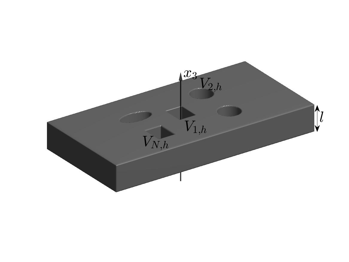
a) b)

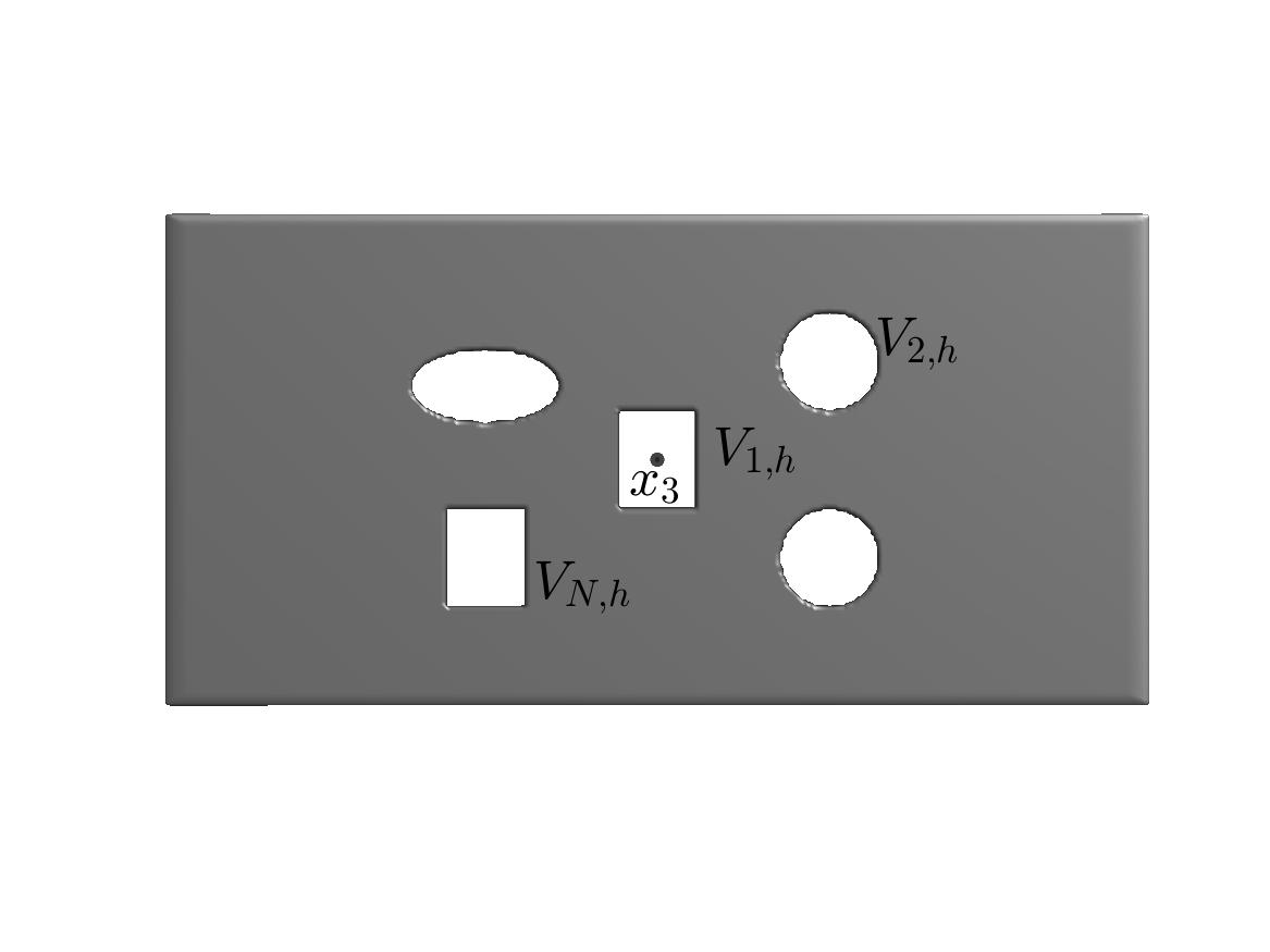
Figure 1: A sound-hard slab of thickness $l$ with $N$ cylindrical holes $\{V_{j,h}\}_{j=1}^{N}$: (a) side view; (b) top-view.

let $\{V_{j,h}\}_{j=1}^{N}$ denotes the set of $N$ holes in a sound-hard slab of thickness $l$. Throughout this paper, we assume that $\{V_{j,h}\}_{j=1}^{N}$ satisfies the following conditions: (1) $\{V_{j,h}\}_{j=1}^{N}$ are cylindrical, i.e. $x_{3}$-independent; (2) $\{V_{j,h}\}_{j=1}^{N}$ are generated respectively by two-dimensional, simple-connected Lipschitz domains $\{G_{j}\}_{j=1}^{N}$, all of which contain the origin point $(0,0)$, and the small parameter $h\ll 1$, through

$$V_{j,h}=\{(x_{1},x_{2},x_{3})\in\mathbb{R}^{3}:(x_{1},x_{2})\in D_{j}+hG_{j},x_{3}\in(-l,0)\},$$

where $D_{j}+hG_{j}=\{D_{j}+(hx_{1},hx_{2})\in\mathbb{R}^{2}:(x_{1},x_{2})\in G_{j}\}$, $\{D_{j}\}_{j=1}^{N}$ are well-separated points in $\mathbb{R}^{2}$ so that $C_{j}=(D_{j},-l/2)$ become the center of $V_{j,h}$; (3) the area of $G_{j}$ is $1$. Here, condition (3) is not necessary and is only introduced to simplify the presentation. Let $\Gamma_{j,h}=\partial V_{j,h}\cap\{x:x_{3}=0\}$ denotes the top boundary of $V_{j,h}$, which will be called the aperture of $V_{j,h}$ in the following.

In such a 3D structure, a sound field outside the holes $\{V_{j,h}\}$ can be expressed in terms of its normal derivatives on the apertures $\{G_{j,h}\}$. Inside each hole $V_{j,h}$, since the vertical variable can be separated, the field can be expressed in terms of a countable set of Fourier basis functions. Matching the field on each aperture $G_{j,h}$ yields a linear system of countable equations in terms of a countable set of unknown Fourier coefficients. The linear system can be reduced to a finite-dimensional linear system based on the invertibility of a principal submatrix, which is proved by establishing the well-posedness of a closely related boundary value problem for each hole $V_{j,h}$ in the limiting case $h\to 0$, so that only the leading Fourier coefficient for each hole $V_{j,h}$ is preserved in the finite-dimensional system. In other words, the resonance frequencies are those making the resulting $N$-dimensional linear system rank deficient. By regular asymptotic analysis, we get a systematic asymptotic formula for characterizing the resonance frequencies of the 3D structure. The formula reveals an important fact that when all holes are of the same shape, the quality factor $Q$ for any resonance frequency asymptotically behaves as ${\cal O}(h^{-2})$ for $h\ll 1$, the prefactor of which depends only on the locations of holes, but is independent of the shape.

1.1 Notations and Equivalent Sobolev norms

For any Lipschitz domain $\Omega\in\mathbb{R}^{n},n=2,3$, let $L^{2}(\Omega)$ denote the set of all square-integrable functions on $\Omega$ equipped with the usual inner product: for any $f,g\in L^{2}(\Omega)$,

$$(f,g)_{L^{2}(\Omega)}=\int_{\Omega}f\bar{g}dx.$$

Let $H^{1}(\Omega)=\{f\in L^{2}(\Omega):\nabla f\in(L^{2}(\Omega))^{3}\}$ be equipped with the standard inner product: for any $f,g\in H^{1}(\Omega)$,

$$(f,g)_{H^{1}(\Omega)}=\int_{\Omega}f\bar{g}+\nabla f\cdot\nabla\bar{g}dx.$$

Let $\tilde{H}^{-1}(\Omega)$ denote the dual space of $H^{1}(\Omega)$. Then, the interpolation theory can help us to define the fractional Sobolev space $H^{1/2}(\Omega)$ and its dual space $\tilde{H}^{-1/2}(\Omega)$. Let $\ell^{2}=\{\{f_{m}\}_{m=0}^{\infty}\subset\mathbb{C}:\sum_{m=0}^{\infty}|f_{m}|^{2}<\infty\}$ be equipped with its natural inner product: for any $\{f_{m}\}_{m=0}^{\infty},\{g_{m}\}_{m=0}^{\infty}\in\ell^{2}$:

$$<\{f_{m}\},\{g_{m}\}>_{\ell^{2}}=\sum_{m=0}^{\infty}f_{m}\bar{g}_{m}.$$

For any $f\in H^{1/2}(\Omega)$ and $g\in\tilde{H}^{-1/2}(\Omega)$, the duality pair $<f,g>_{H^{1/2}(\Omega),\tilde{H}^{-1/2}(\Omega)}$, understood as the functional $f$ acting on $g$, will be abbreviated as $<f,g>_{1/2,-1/2}$ for simplicity when the definition domain of $f$ or $g$ is clear from the context; similarly, $<g,f>_{-1/2,1/2}$ denotes the functional $g\in\tilde{H}^{-1/2}(\Omega)=(H^{1/2}(\Omega))^{\prime}$ acting on element $f\in H^{1/2}(\Omega)$. Certainly, $<f,g>_{1/2,-1/2}=\overline{<g,f>_{-1/2,1/2}}$ and becomes $(f,g)_{L^{2}(\Omega)}$ when $g\in L^{2}(\Omega)$.

To simply characterize the aforementioned fractional Sobolev spaces on the aperture boundary $\Gamma_{j,h}$ of the hole $V_{j,h}$, we rely on the following theorem regarding spectral properties of the 2D Laplacian $\Delta_{2}=\partial_{x_{1}}^{2}+\partial_{x_{2}}^{2}$ on the Lipschitz domains $\{G_{j}\}_{j=1}^{N}$.

Theorem 1.1 (See Theorem 4.12 in [25]).

For the 2D Lipschitz domain $\{G_{j}\}_{j=1}^{N}$ generating the $N$ holes $\{V_{j,h}\}_{j=1}^{N}$, respectively, there exist sequences of functions $\phi_{1,j},\phi_{2,j},\cdots,$ in $H^{1}(G_{j})$, and of nonnegative numbers $\lambda_{0,j},\lambda_{1,j},\cdots,$ having the following properties:

• Each $\phi_{m,j}$ is an eigenfunction of $-\Delta_{2}$ with eigenvalue $\lambda_{m,j}$:

  $$-\Delta_{2}\phi_{m,j}= \lambda_{m,j}\phi_{m,j},\quad{\rm on}\quad G_{j},$$

  $$\partial_{\nu}\phi_{m,j}= 0,\quad{\rm on}\quad\partial G_{j}.$$

• The eigenvalues satisfy $0=\lambda_{0,j}<\lambda_{1,j}\leq\lambda_{2,j}\leq\cdots$ with $\lambda_{m,j}\to\infty$ as $i\to\infty$.

• The eigenfunctions $\{\phi_{m,j}\}_{i=0}^{\infty}$ form a complete orthonormal system in $L_{2}(G_{j})$, and in particular $\phi_{0,j}=1$.

• For any $f\in H^{1}(G_{j})$,

  $$||f||_{H^{1}(G_{j})}^{2}\eqsim\sum_{m=0}^{\infty}(1+\lambda_{m,j})|(f,\phi_{m,j})_{L^{2}(G_{j})}|^{2}.$$

Proof.

The only difference from Theorem 4.12 of [25] is $\lambda_{0,j}=0$, $\lambda_{1,j}>0$ and $\phi_{0,j}=1$. This can be seen that all eigenvalues must be nonnegative by testing the governing equation with $\phi_{m,j}$ themselves. On the other hand, for $\lambda_{0,j}=0$, $\phi_{0,j}=1$ is the unique up to a sign and normalized (see condition (3) about $G_{j}$) solution of the eigenvalue problem so that $\lambda_{m,j}>0$ for $i\geq 1$. ∎

Based on Theorem 1.1(iii), on each aperture $\Gamma_{j,h}=(D_{j}+hG_{j})\times\{x_{3}=l\}$,

$$\{\phi_{m,j}(\cdot;h)=h^{-1}\phi_{m,j}((\cdot-D_{j})/h)\}_{m=0}^{\infty},$$

forms a complete and orthonormal basis of $L^{2}(\Gamma_{j,h})$, so that for any $f\in L^{2}(\Gamma_{j,h})$, the set of Fourier coefficients,

$$\{f_{m,j}=(f,\phi_{m,j}(\cdot;h))_{L^{2}(\Gamma_{j},h)}\}_{m=0}^{\infty}\in\ell^{2}.$$

By Parserval’s identity,

$$||f||_{L^{2}(\Gamma_{j,h})}=||\{f_{m}\}||_{\ell^{2}}=\left(\sum_{m=0}^{\infty}|f_{m}|^{2}\right)^{1/2}.$$

On the other hand, Theorem 1.1(iv) indicates that, the $H^{1}(\Gamma_{j,h})$ can be equipped with the following equivalent norm: for any $f\in H^{1}(\Gamma_{j,h})$,

$$||f||_{H^{1}(\Gamma_{j,h})}=\left(\sum_{m=0}^{\infty}(1+\lambda_{m})|f_{m}|^{2}\right)^{1/2}.$$

Now by interpolation theory, $H^{1/2}(\Gamma_{j,h})$ can be equipped with the following equivalent norm

$$||f||_{H^{1/2}(\Gamma_{j,h})}=\left(\sum_{m=0}^{\infty}(1+\lambda_{m,j})^{1/2}|f_{m}|^{2}\right)^{1/2},$$

so that its dual space $\tilde{H}^{-1/2}(\Gamma_{j,h})$ is equipped with

$$||f||_{\tilde{H}^{-1/2}(\Gamma_{j,h})}=\left(\sum_{m=0}^{\infty}(1+\lambda_{m,j})^{-1/2}|f_{m}|^{2}\right)^{1/2},$$

where $f_{m}$ should be redefined as $<f,\phi_{m}>_{-1/2,1/2}$ now.

The rest of this paper is organized as follows. In section 2, we study resonances by a sound-soft slab with a single hole, and analyze the mechanism of field enhancement near resonance frequencies. In section 3, we extend the approach to study resonances of a slab with multiple slits and provide an accurate asymptotic formula of the resonance frequencies. Finally, we draw the conclusion and present some potential applications of the current method.

2 Single cylindrical hole

To clarify the basic idea, we begin with a slab of thickness $l$ with a single cylindrical hole, say $V_{1,h}$, for $h\ll 1$. For simplicity, we assume $D_{1}=(0,0)$ so that $C_{1}=(0,0,-l/2)$ in this section. We seek a complex frequency $k$ such that there exists a nonzero outgoing sound wave field $u$ satisfies the following three-dimensional Helmholtz equation

$$\Delta u+k^{2}u =0,\quad{\rm on}\ \Omega_{h},$$ (1)

$$\partial_{\nu}u =0,\quad{\rm on}\ \partial\Omega_{h},$$ (2)

where $\Omega_{h}$ is the interior of $\{x\in\mathbb{R}^{3}:x_{1},x_{2}\in\mathbb{R},x_{3}\notin[-l,0]\}\cup\overline{V_{1,h}}$. The searching region ${\cal B}=\{k\in\mathbb{C}:{\rm Re}(k)>0,{\rm Im}(k)<0,|k|\in(\epsilon_{0},K)\}$ for some sufficiently small constant $\epsilon_{0}>0$ and some sufficiently large constant $K>0$. Similar as in [33], we consider even modes and odd modes symmetric about $x_{3}=-l/2$.

2.1 Even modes

Suppose now $u$ is an even function about $x_{3}=-l/2$, i.e., $u(x_{1},x_{2},x_{3})=u(x_{1},x_{2},-l-x_{3})$, so that the original problem is reduced to the following half-space problem: find a solution $u\in H^{1}_{\rm loc}(\Omega_{h}^{+})$ solving

$$\Delta u+k^{2}u =0,\quad{\rm on}\ \Omega_{h}^{+},$$ (3)

$$\partial_{\nu}u =0,\quad{\rm on}\ \partial\Omega_{h}^{+},$$ (4)

where $\Omega_{h}^{+}=\mathbb{R}_{+}^{3}\cup V_{1,h}^{+}\cup\Gamma_{1,h}$, $V_{1,h}^{+}=V_{1,h}\cap\{x\in\mathbb{R}^{3}:x_{3}\in(-l/2,0)\}$ and we recall that $\Gamma_{1,h}$ denotes the aperture surface, as shown in Figure 2.

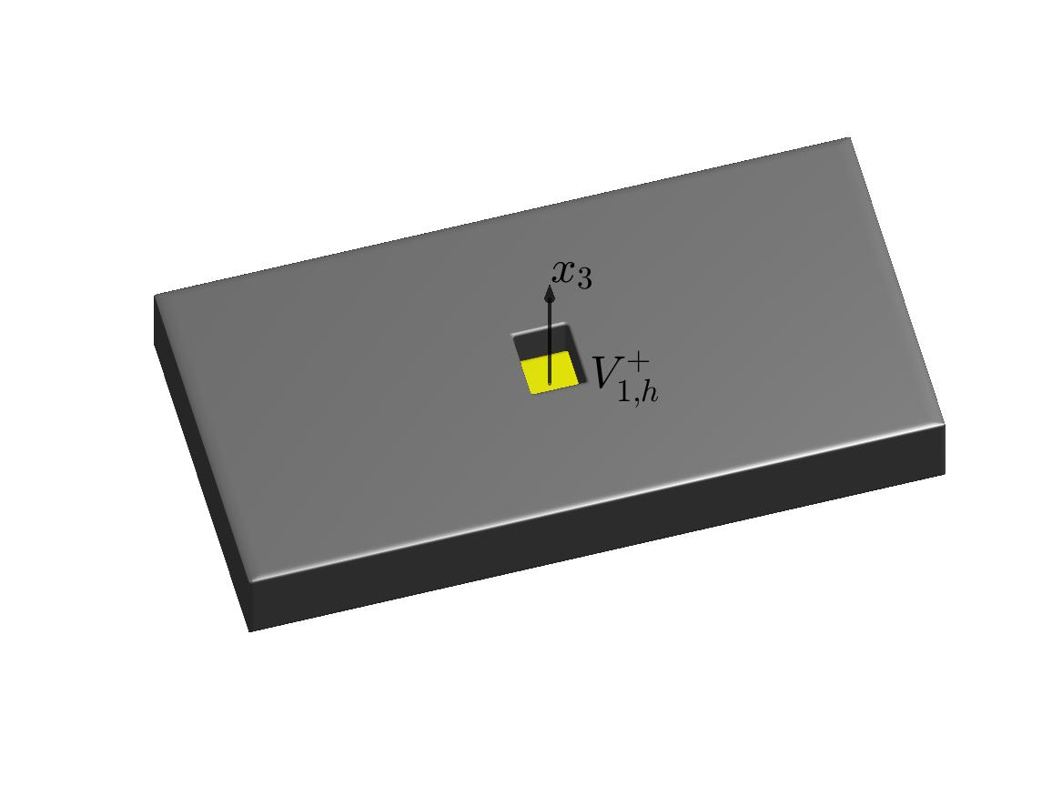
a) b)

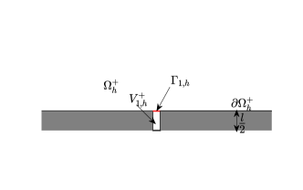
Figure 2: A half-plane problem with one cylindrical cavity $V_{1,h}^{+}$: (a) side view; (b) the cross-section at $x_{1}=0$.

Recall from Theorem 1.1 that

$$\{\phi_{m,1}(x;h)=h^{-1}\phi_{m,1}((x-C_{1})/h)\}_{m=0}^{\infty},$$

form a complete and orthonormal basis in $L^{2}(\Gamma_{h})$, and the corresponding eigenvalues are $\{\lambda_{m,1}\}_{m=2}^{\infty}$. To simplify the presentation, we shall suppress the label $1$ so that $V_{h}^{+}=V_{1,h}^{+}$, etc..

Since $u|_{\Gamma_{h}}\in H^{1/2}(\Gamma_{h})$, there exists a sequence $\{b_{m}\}_{m=0}^{\infty}$ such that

$$u|_{\Gamma_{h}}=\sum_{m=0}^{\infty}b_{m}\phi_{m}(x;h)[e^{{\bf i}s_{m}l}+1],$$ (5)

with

$$\sum_{m=0}^{\infty}(1+\lambda_{m})^{1/2}|b_{m}(e^{{\bf i}s_{m}l}+1)|^{2}<\infty,$$

where

$$s_{m}= \sqrt{k^{2}-\frac{\lambda_{m}}{h^{2}}}.$$ (6)

Therefore, $\{a_{m}=\lambda_{m}^{1/2}b_{m}\}_{m=0}^{\infty}\in\ell^{2}$ for $h\ll 1$ since

$$\sum_{m=0}|a_{m}|^{2}\leq C\sum_{m=0}^{\infty}(1+\lambda_{m})^{1/2}|b_{m}(e^{{\bf i}s_{m}l}+1)|^{2}<\infty.$$

In $V_{h}^{+}$, define

$$u^{-}(x)=\sum_{m=0}^{+\infty}b_{m}\phi_{m}(x;h)[e^{{\bf i}s_{m}(x_{3}+l)}+e^{-{\bf i}s_{m}x_{3}}].$$ (7)

We could verify that $\phi=u-u^{-}\in H^{1}(V_{h}^{+})$ solves

$$\Delta\phi= -k^{2}\phi,\quad{\rm on}\quad V_{h}^{+},$$ (8)

$$\partial_{\nu}\phi= 0,\quad{\rm on}\quad\partial V_{h}^{+}\backslash\overline{\Gamma_{h}},$$ (9)

$$\phi= 0,\quad{\rm on}\quad\Gamma_{h}.$$ (10)

When $k\in{\cal B}$ and $h\ll 1$, $-k^{2}$ is not an eigenvalue of the above problem so that we have $u=u^{-}$ on $C_{h}^{+}$. Therefore, its normal derivative on $\Gamma_{h}$ becomes

$$\partial_{\nu}u(x)=\partial_{x_{3}}u(x_{1},x_{2},0)=\sum_{m=0}^{+\infty}b_{m}{\bf i}s_{m}\phi_{m}(x;h)[e^{{\bf i}s_{m}l}-1]\in\tilde{H}^{-1/2}(\Gamma_{h}).$$ (11)

When $e^{{\bf i}s_{0}l}+1=0$, the representation (5) of $u|_{\Gamma_{h}}$ is impossible to define $b_{0}$. To resolve this issue, we could choose (11) to define all $\{b_{m}\}_{m=0}^{\infty}$ so that the representation (7) becomes valid for all finite frequencies $k\in{\cal B}$ and $h\ll 1$.

Let $\epsilon=kh\ll 1$ since $k\in{\cal B}$ and $h\ll 1$. We define the following integral operators:

$$[{\cal S}\phi](x)= \int_{\Gamma_{h}}\frac{e^{{\bf i}k|x-y|}}{2\pi|x-y|}\phi(y)dS(y),\quad x\in\Gamma_{h},$$ (12)

$$[{\cal S}_{0}\phi](x)= \int_{\Gamma_{1}}\frac{1}{2\pi|x-y|}\phi(y)dS(y),\quad x\in\Gamma_{1},$$ (13)

$$[{\cal R}_{0}\phi](x)= \int_{\Gamma_{1}}\frac{e^{{\bf i}\epsilon|x-y|}-1-{\bf i}\epsilon|x-y|}{2\pi\epsilon^{2}|x-y|}\phi(y)dS(y),\quad x\in\Gamma_{1},$$ (14)

where $\Gamma_{1}=G_{1}\times\{0\}$ is the aperture surface $\Gamma_{h}$ when $h=1$. Some important properties of the above integral operators are listed below.

Lemma 2.1.

For any $k\in{\cal B}$ and $h\ll 1$, we have:

• ${\cal S}$ can be uniquely extended as a bounded operator from $\tilde{H}^{-1/2}(\Gamma_{h})$ to $H^{1/2}(\Gamma_{h})$;

• ${\cal S}_{0}$ can be uniquely extended as a bounded operator from $\tilde{H}^{-1/2}(\Gamma_{1})$ to $H^{1/2}(\Gamma_{1})$, and ${\cal S}_{0}$ is positive and bounded below on $\tilde{H}^{-1/2}(\Gamma_{1})$, i.e., for any $\phi\in\tilde{H}^{-1/2}(\Gamma_{1})$,

  $$<{\cal S}_{0}\phi,\phi>_{1/2,-1/2}\geq C||\phi||_{\tilde{H}^{-1/2}(\Gamma_{1})},$$

  for some positive constant $C>0$.

• ${\cal R}_{0}$ can be uniquely extended as a uniformly bounded operator from $\tilde{H}^{-1/2}(\Gamma_{1})$ to $H^{1/2}(\Gamma_{1})$, i.e.,

  $$||{\cal R}_{0}||\leq C,$$

  for some constant $C>0$ independent of $\epsilon$.

Proof.

Choosing any bounded and closed Lipschitz surface $\Gamma_{c}\subset\overline{\mathbb{R}_{+}^{3}}$ that contains $\Gamma_{1}$, we can extend ${\cal S}_{0}$ as for any $\phi\in\tilde{H}^{-1/2}(\Gamma_{1})\subset H^{-1/2}(\Gamma_{c})$,

$${\cal S}_{0}\phi=(2{\cal S}_{c}\phi)|_{\Gamma_{1}},$$

where

$${\cal S}_{c}\phi=\int_{\Gamma_{c}}G_{0}(x,y)\phi(y)dS(y),$$

with the three dimensional fundamental solution $G_{0}(x,y)=\frac{1}{4\pi|x-y|}$ of Laplacian as the kernel. According to [25, Thm. 7.6 & Cor. 8.13], it is clear that ${\cal S}_{c}$ is bounded from $H^{-1/2}(\Gamma_{c})$ to $H^{1/2}(\Gamma_{c})$, and satisfies for any $\psi\in H^{-1/2}(\Gamma_{c})$,

$$<{\cal S}_{c}\psi,\psi>_{H^{1/2}(\Gamma_{c}),H^{-1/2}(\Gamma_{c})}\geq C||\psi||_{H^{-1/2}(\Gamma_{c})}/2,$$

for some constant $C>0$. Thus, for any $\phi\in\tilde{H}^{-1/2}(\Gamma_{1})$, ${\cal S}_{0}\phi\in H^{1/2}(\Gamma_{1})$ so that

$$<{\cal S}_{0}\phi,\phi>_{H^{1/2}(\Gamma_{1}),H^{-1/2}(\Gamma_{1})}=<2{\cal S}_{c}\phi,\phi>_{H^{1/2}(\Gamma_{c}),H^{-1/2}(\Gamma_{c})}\geq C||\phi||_{\tilde{H}^{-1/2}(\Gamma_{1})}.$$

The mapping property of ${\cal S}$ on $\Gamma_{h}$ can be similarly obtained. Now we prove the uniform boundedness of ${\cal R}_{0}$. Since the kernel function of ${\cal R}_{0}$ in (14) and its gradient with respect to $x$ are uniformly bounded for all $k\in{\cal B}$ and $h\ll 1$, we easily conclude that ${\cal R}_{0}$ is uniformly bounded from $L^{2}(\Gamma_{1})$ to $H^{1}(\Gamma_{1})$. The self-adjointness of ${\cal R}_{0}$ and interpolation theory then indicate the uniform boundedness of ${\cal R}_{0}$ mapping from $\tilde{H}^{-1/2}(\Gamma_{1})$ to $H^{1/2}(\Gamma_{1})$. ∎

In the upper half plane $\mathbb{R}_{+}^{3}$, the Neumann data $\partial_{\nu}u(x)=-\partial_{x_{3}}u(x)$ in $\tilde{H}^{-1/2}(\Gamma_{h})$ uniquely determines the following outgoing solution

$$u(x)=-\int_{\Gamma_{h}}\frac{e^{{\bf i}k|x-y|}}{2\pi|x-y|}\partial_{x_{3}}u(y)dS(y)\in H^{1}_{\rm loc}(\mathbb{R}_{+}^{3}),\quad{\rm on}\quad\mathbb{R}_{+}^{3},$$

with trace $u|_{\Gamma_{h}}=-{\cal S}\partial_{x_{3}}u\in H^{1/2}(\Gamma_{h})$ by Lemma 2.1. By the continuity of $\partial_{\nu}u$ on $\Gamma_{h}$, to ensure that $u\in H^{1}_{\rm loc}(\Omega_{h}^{+})$, we require that

$$u|_{\Gamma_{h}}=-{\cal S}\partial_{x_{3}}u=\sum_{m=0}^{\infty}b_{m}\phi_{m}(x;h)[e^{{\bf i}s_{m}l}+1]\in H^{1/2}(\Gamma_{h}),$$

which is equivalent to for any nonnegative integers $m$,

$$(-{\cal S}\partial_{x_{3}}u,\phi_{m}(x_{1},x_{2};h))_{L^{2}(\Gamma_{h})}=b_{m}[e^{{\bf i}s_{m}l}+1].$$

By (11), the above equations can be rewritten as the following infinite number of linear equations in terms of unknowns $\{b_{0},\{a_{m}\}\}\in\ell^{2}$, i.e.,

$$b_{0}[e^{{\bf i}s_{0}l}+1]= -b_{0}{\bf i}s_{0}h[e^{{\bf i}s_{0}l}-1]d_{00}-\sum_{m^{\prime}=1}^{\infty}a_{m^{\prime}}\lambda_{m^{\prime}}^{-1/4}{\bf i}s_{m^{\prime}}h[e^{{\bf i}s_{m^{\prime}}l}-1]d_{m^{\prime}0},$$ (15)

$$\lambda_{m}^{-1/4}a_{m}[e^{{\bf i}s_{m}l}+1]= -b_{0}{\bf i}s_{0}h[e^{{\bf i}s_{0}l}-1]d_{0m}-\sum_{m^{\prime}=1}^{\infty}a_{m^{\prime}}\lambda_{m^{\prime}}^{-1/4}{\bf i}s_{m^{\prime}}h[e^{{\bf i}s_{m^{\prime}}l}-1]d_{m^{\prime}m},$$ (16)

where we have set for integers $m^{\prime},m\geq 0$ that

$$d_{m^{\prime}m}=h^{-1}({\cal S}\phi_{m^{\prime}}(\cdot;h),\phi_{m}(\cdot;h))_{L^{2}(\Gamma_{h})}.$$ (17)

We have the following properties regarding asymptotics of $d_{m^{\prime}m}$ as $\epsilon\ll 1$.

Lemma 2.2.

For $\epsilon\ll 1$ and for nonnegative integers $m,m^{\prime}$, $d_{m^{\prime}m}$ asymptotically behaves as following:

$$d_{m^{\prime}m}=\left\{\begin{array}[]{ll}({\cal S}_{0}1,1)_{L^{2}(\Gamma_{1})}+\frac{{\bf i}\epsilon}{2\pi}+{\cal O}(\epsilon^{2}),&m=m^{\prime}=0;\\ ({\cal S}_{0}\phi_{m^{\prime}},\phi_{m})_{L^{2}(\Gamma_{1})}+\epsilon^{2}({\cal R}_{0}\phi_{m^{\prime}},\phi_{m})_{L^{2}(\Gamma_{1})},&{\rm otherwise},\end{array}\right.$$ (20)

where $\phi_{m}$ is short for $\phi_{m}(\cdot;h)$ when $h=1$.

Proof.

By rescaling,

$$d_{m^{\prime}m}= \frac{1}{2\pi}\int_{\Gamma_{1}}\int_{\Gamma_{1}}\frac{e^{{\bf i}\epsilon|x-y|}}{|x-y|}\phi_{m^{\prime}}(y;1)dS(y)\bar{\phi}_{m}(x;1)dS(x),$$

$$= ({\cal S}_{0}\phi_{m^{\prime}},\phi_{m})_{L^{2}(\Gamma_{1})}+\frac{{\bf i}\epsilon}{2\pi}\int_{\Gamma_{1}}\int_{\Gamma_{1}}\phi_{m^{\prime}}(y;1)dy_{1}dy_{2}\bar{\phi}_{m}(x;1)dx_{1}dx_{2}+\epsilon^{2}({\cal R}_{0}\phi_{m^{\prime}},\phi_{m})_{L^{2}(\Gamma_{1})}.$$

It is clear that the second term of the r.h.s is nonzero only when $m=m^{\prime}=0$. ∎

Now set for $m>0$ and $m^{\prime}>0$ that

$$c_{00}= -{\bf i}\epsilon d_{00},$$ (21)

$$c_{m^{\prime}0}= -\lambda_{m^{\prime}}^{-1/4}{\bf i}s_{m^{\prime}}h[e^{{\bf i}s_{m^{\prime}}l}-1]d_{m^{\prime}0},$$ (22)

$$c_{0m}= -\lambda_{m}^{1/4}\frac{{\bf i}\epsilon}{e^{{\bf i}s_{m}l}+1}d_{0m},$$ (23)

$$c_{m^{\prime}m}= -\lambda_{m^{\prime}}^{-1/4}\lambda_{m}^{1/4}{\bf i}s_{m^{\prime}}h\frac{e^{{\bf i}s_{m^{\prime}}l}-1}{e^{{\bf i}s_{m}l}+1}d_{m^{\prime}m},$$ (24)

we could rewrite the previous linear equations (15) and (16) more compactly in the following form,

$$b_{0}[e^{{\bf i}s_{0}l}+1]= b_{0}[e^{{\bf i}s_{0}l}-1]c_{00}+<\{a_{m^{\prime}}\},\{c_{m^{\prime}0}\}>_{\ell^{2}},$$ (25)

$$\{a_{m}\}= b_{0}[e^{{\bf i}s_{0}l}-1]\{c_{0m}\}+{\cal A}_{h}\{a_{m}\},$$ (26)

where the operator ${\cal A}_{h}$ is defined as: for any $\{f_{m}\}_{m=1}^{\infty}\in\ell^{2}$,

$${\cal A}_{h}\{f_{m}\}_{m=1}^{\infty}=\{\sum_{m=1}^{\infty}c_{m^{\prime}m}f_{m^{\prime}}\}_{m=1}^{\infty},$$ (27)

According to Lemma 2.2, we have the following properties.

Lemma 2.3.

For $h\ll 1$ and $k\in{\cal B}$:

• $$c_{00}=-({\cal S}_{0}1,1)_{L^{2}(\Gamma_{1})}\epsilon{\bf i}+\frac{\epsilon^{2}}{2\pi}+{\cal O}(\epsilon^{3});$$

• When $m>0$,

  $$c_{0m}=-{\bf i}\epsilon({\cal S}_{0}1,\lambda_{m}^{1/4}\phi_{m})_{L^{2}(\Gamma_{1})}-{\bf i}\epsilon^{3}({\cal R}_{0}1,\lambda_{m}^{1/4}\phi_{m})_{L^{2}(\Gamma_{1})},$$

  and $\{c_{0m}\}_{m=1}^{\infty}\in\ell^{2}$;

• When $m^{\prime}>0$,

  $$c_{m^{\prime}0}= -({\cal S}_{0}1,\lambda_{m^{\prime}}^{1/4}\phi_{m^{\prime}})_{L^{2}(\Gamma_{1})}-\epsilon^{2}({\cal R}_{0}1,\lambda_{m^{\prime}}^{1/4}\phi_{m^{\prime}n^{\prime}})_{L^{2}(\Gamma_{1})}+({\cal S}_{0}1,\lambda_{m^{\prime}}^{-3/4}\phi_{m^{\prime}n^{\prime}}){\cal O}(\epsilon^{2}),$$

  and $\{c_{m^{\prime}0}\}_{m^{\prime}=1}^{\infty}\in\ell^{2}$;

• When $m^{\prime},m>0$,

  $$c_{m^{\prime}m}= -({\cal S}_{0}\lambda_{m^{\prime}}^{1/4}\phi_{m^{\prime}},\lambda_{m}^{1/4}\phi_{m})_{L^{2}(\Gamma_{1})}-\epsilon^{2}({\cal R}_{0}\lambda_{m^{\prime}}^{1/4}\phi_{m^{\prime}},\lambda_{m}\phi_{m})_{L^{2}(\Gamma_{1})}+({\cal S}_{0}\lambda_{m^{\prime}}^{-3/4}\phi_{m^{\prime}},\lambda_{m}^{1/4}\phi_{m})_{L^{2}(\Gamma_{1})}{\cal O}(\epsilon^{2}),$$

  and the operator ${\cal A}_{h}$ defined by $\{c_{m^{\prime}m}\}_{m,m^{\prime}>0}$ is bounded from $\ell^{2}$ to $\ell^{2}$ and can be decomposed as

  $${\cal A}_{h}={\cal P}+\epsilon^{2}{\cal Q}_{h},$$ (28)

  where ${\cal P}$ is defined as

  $${\cal P}\{f_{m}\}_{m>0}=\left\{-\sum_{m^{\prime}>0}({\cal S}_{0}\lambda_{m^{\prime}}^{1/4}\phi_{m^{\prime}},\lambda_{m}^{1/4}\phi_{m})_{L^{2}(\Gamma_{1})}f_{m}\right\}_{m>0},$$

  and ${\cal Q}_{h}=\epsilon^{-2}({\cal A}_{h}-{\cal P})$. Both ${\cal P}$ and ${\cal Q}_{h}$ are uniformly bounded from $\ell^{2}$ to $\ell^{2}$ for all $k\in{\cal B}$ and $h\ll 1$.

Proof.

The asymptotic behaviors of $\{c_{m^{\prime}m}\}_{m,m^{\prime}>0}$ are trivial by Lemma 2.2. As for the other properties, we here only show that the leading terms of $\{c_{m^{\prime}m}\}$ satisfy those properties as the high-order terms can be analyzed similarly. For any $\{f_{m}\}_{m>0}\in\ell^{2}$ and $\{g_{m}\}_{m>0}\in\ell^{2}$, the following two functions

$$f=\sum_{m>0}f_{m}\lambda_{m}^{1/4}\phi_{m},\ {\rm and}\ g=\sum_{m>0}f_{m}\lambda_{m}^{1/4}\phi_{m},$$

are in $H^{-1/2}(\Gamma_{1})$. We thus have

$$|\sum_{m>0}({\cal S}_{0}1,\lambda_{m}^{1/4}\phi_{m})_{L^{2}(\Gamma_{1})}\bar{f}_{m}|$$

$$= |<-{\cal S}_{0}1,f>_{1/2,-1/2}|\leq||{\cal S}_{0}1||_{H^{1/2}(\Gamma_{1})}||f||_{H^{-1/2}(\Gamma_{1})}\leq||{\cal S}_{0}1||_{H^{1/2}(\Gamma_{1})}||\{f_{m}\}||_{\ell^{2}},$$

indicating that $\{c_{0m}\}\in\ell^{2}$ and $\{c_{m^{\prime}0}\}\in\ell^{2}$. Moreover,

$$\left|\sum_{m>0}\sum_{m^{\prime}>0}-({\cal S}_{0}\lambda_{m^{\prime}}^{1/4}\phi_{m^{\prime}},\lambda_{m}^{1/4}\phi_{m})_{L^{2}(\Gamma_{1})}f_{m^{\prime}}g_{m}\right|$$

$$= |<{\cal S}_{0}f,g>_{1/2,-1/2}|\leq||{\cal S}_{0}||\cdot||\{f_{m}\}||_{\ell^{2}}||g_{m}||_{\ell^{2}},$$

which implies the mapping property of ${\cal A}_{h}$ as well as the boundedness. ∎

2.1.1 Invertibility of ${\cal I}-{\cal A}_{h}$

To prove ${\cal I}-{\cal A}_{h}$ has a bounded inverse for $h\ll 1$, we no longer justify the diagonal dominance of the infinite-dimensional matrix $\{\delta_{m^{\prime}m}-c_{m^{\prime}m}\}_{m^{\prime},m=0}^{\infty}$ as was done in [33], since now $c_{m^{\prime}m}$ is challenging to accurately approximate, although we conjecture that this property remains true. To resolve this issue, we convert the study of the invertibility of ${\cal I}-{\cal A}_{h}$ to the study of the well-posedness of a closely related boundary-value problem in a semi-infinite cylinder $\Omega^{-}=G_{1}\times\mathbb{R}^{-}$, as was done in [5]. Nevertheless, compared with the two-dimensional proof in [5], our three-dimensional proof is simpler, more versatile, and more straightforward due to the following aspects: (1) we make no use of the Green function of $\Omega^{-}$, which is complicated; (2) it is not necessary to introduce a Dirichlet-to-Neumann map to truncate the unbounded cylinder $\Omega^{-}$; (3) the proof does not use any particular property regarding the shape of $\Omega^{-}$ (e.g. a circular hole in [18] or a rectangular hole).

As seen in Lemma 2.3, ${\cal P}$ can be regarded as the limit of ${\cal A}_{h}$ as $h\to 0$ so that by Neumann series, we could see that ${\cal I}-{\cal A}_{h}$ is invertible if ${\cal I}-{\cal P}$ is invertible. The open mapping theorem implies the following lemma.

Lemma 2.4.

For $k\in{\cal B}$ and $h\ll 1$, the operator ${\cal I}-{\cal P}:\ell^{2}\to\ell^{2}$ has a bounded inverse, if for any $\{\alpha_{m}\}_{m>0}\in\ell^{2}$, the following problem

$${\rm(P1):}\quad\{a_{m}\}_{m>0}={\cal P}\{a_{m}\}_{m>0}+\{\alpha_{m}\}_{m>0},$$

has a unique solution $\{a_{m}\}_{m>0}\in\ell^{2}$.

For $\{\alpha_{m}\}_{m>0}\in\ell^{2}$, let

$$\beta_{m}= \alpha_{m}\lambda_{m}^{-1/4},\quad m>0,$$ (29)

$$f(x_{1},x_{2})= \sum_{m>0}\beta_{m}\phi_{m}(x),\quad|x_{i}|\leq 1/2,i=1,2.$$ (30)

Let $H_{0}^{1/2}(\Gamma_{1})=\{\phi\in H^{1/2}(\Gamma_{1}):(\phi,1)_{L^{2}(\Gamma_{1})}=0\}$ and $\tilde{H}_{0}^{-1/2}(\Gamma_{1})=\{\phi\in\tilde{H}^{-1/2}(\Gamma_{1}):<\phi,1>_{-1/2,1/2}=0\}$. It can be seen that $f\in H_{0}^{1/2}(\Gamma_{1})$. Now, consider the following problem:

$${\rm(P2):}\quad\left\{\begin{array}[]{ll}\Delta u=0,&{\rm on}\quad\Omega^{-}=G_{1}\times\mathbb{R}^{-},\\ \partial_{\nu}u=0,&{\rm on}\quad\partial\Omega^{-}\backslash\overline{\Gamma_{1}},\\ u+{\cal S}_{0}\partial_{\nu}u=f+<S_{0}\partial_{\nu}u-f,1>_{1/2,-1/2},&{\rm on}\quad\Gamma_{1},\\ \end{array}\right.$$

We have the following lemma.

Lemma 2.5.

For any $\{\alpha_{m}\}_{m>0}\in\ell^{2}$, problem (P1) has a unique solution $\{a_{m}\}_{m>0}\in\ell^{2}$ iff problem (P2) has a unique solution $u\in H^{1}(\Omega^{-})$ for any $f\in H_{0}^{1/2}(\Gamma_{1})$ defined in (30).

Proof.

Given $\{\alpha_{m}\}_{m>0}\in\ell^{2}$, suppose (P1) has a solution $\{a_{m}\}_{m>0}\in\ell^{2}$. Setting $b_{m}=a_{m}\lambda_{m}^{-1/4}$ for $m>0$, we now claim that

$$u(x)=\sum_{m=1}^{\infty}b_{m}\phi_{m}(x)e^{\lambda_{m}^{1/2}x_{3}}\in H^{1}(\Omega^{-}),$$

and solves (P2). Clearly,

$$||u||_{H^{1}(\Omega^{-})}\eqsim \int_{-\infty}^{0}dx_{3}\int_{G_{1}}|u(x_{1},x_{2},x_{3})|^{2}+|\partial_{x_{1}}u(x_{1},x_{2},x_{3})|^{2}+|\partial_{x_{2}}u(x_{1},x_{2},x_{3})|^{2}dx_{1}dx_{2}$$

$$+ \int_{-\infty}^{0}dx_{3}\int_{G_{1}}|\partial_{x_{3}}u(x_{1},x_{2},x_{3})|^{2}dx_{1}dx_{2}$$

$$= \int_{-\infty}^{0}dx_{3}||u(\cdot,x_{3})||^{2}_{H^{1}(G_{1})}dx_{1}dx_{2}+\int_{-\infty}^{0}dx_{3}||\partial_{x_{3}}(\cdot,x_{3})||^{2}_{L^{2}(G_{1})}$$

$$\eqsim \int_{-\infty}^{0}\sum_{m>0}^{\infty}(1+\lambda_{m})|b_{m}|^{2}e^{2\lambda_{m}^{1/2}x_{3}}dx_{3}+\int_{-\infty}^{0}\sum_{m>0}\lambda_{m}|b_{m}|^{2}e^{2\lambda_{m}^{1/2}x_{3}}dx_{3}$$

$$= \sum_{m>0}|a_{m}|^{2}\frac{1+2\lambda_{m}}{2\lambda_{m}}<\infty.$$

Now, we verify that $u$ solves (P2). It is clear that $\Delta u=0$ on $\Omega^{-}$ in the distributional sense so that on $\Gamma_{1}$,

$$\partial_{\nu}u=\sum_{m>0}b_{m}\phi_{m}(x)\lambda_{m}^{1/2}\in(H^{1/2}(\Gamma_{1}))^{\prime}=\tilde{H}^{-1/2}(\Gamma_{1}),$$

since $\partial_{\nu}u=0$ on $\partial\Omega^{-}\backslash\overline{\Gamma_{1}}$. Clearly, $<\partial_{\nu}u,1>_{-1/2,1/2}=0$ so that $\partial_{\nu}u\in\tilde{H}^{-1/2}_{0}(\Gamma_{1})$. Thus, it suffices to prove that

$$u+{\cal S}_{0}\partial_{\nu}u=f+<S_{0}\partial_{\nu}u-f,1>_{1/2,-1/2},$$

in $H^{1/2}(\Gamma_{1})$. In fact, for any positive integers $m^{\prime}>0$,

$$<u+{\cal S}_{0}\partial_{\nu}u-f,\phi_{m^{\prime}}>_{1/2,-1/2}= b_{m^{\prime}}+\sum_{m>0}b_{m}\lambda_{m}^{1/2}<{\cal S}_{0}\phi_{m},\phi_{m^{\prime}}>_{1/2,-1/2}-\beta_{m^{\prime}}=0.$$

Conversely, suppose $u\in H^{1}(\Omega^{-})$ solves (P2). We choose for $m>0$,

$$b_{m}=(u|_{\Gamma_{1}},\phi_{m})_{L^{2}(\Gamma_{1})},$$

so that $\{a_{mn}=b_{m}\lambda^{-1/4}\}\in\ell^{2}$ since $u|_{\Gamma_{1}}\in H^{1/2}(\Gamma_{1})$. Now, take

$$u^{*}=\sum_{m>0}b_{m}\phi_{m}(x)e^{\lambda_{m}^{1/2}x_{3}}\in H^{1}(\Omega^{-}),$$

and we claim that $u-u^{*}=0$ on $\Omega^{-}$. In fact, $\phi=u-u^{*}\in H^{1}(\Omega^{-})$ solves

$$\left\{\begin{array}[]{ll}\Delta\phi=0,&{\rm on}\quad\Omega^{-},\\ \phi=0,&{\rm on}\quad\Gamma_{1},\\ \partial_{\nu}\phi=0,&{\rm on}\quad\partial\Omega^{-}\backslash\overline{\Gamma_{1}}.\end{array}\right.$$

Thus, testing the governing equation with $\phi$ itself yields

$$-||\nabla\phi||^{2}_{\Omega^{-}}=0,$$

so that $\phi$ is constant on $\Omega^{-}$. But $\phi|_{\Gamma_{1}}=0$ implies that $\phi=0$. Consequently, following a similar argument as before, we could verify that $\{a_{m}\}_{m>0}$ solves (P1). ∎

To prove that (P2) has a unique solution, we make use of the method of variational formulation. Let

$$V=H^{1}(\Omega^{-})\times\tilde{H}^{-1/2}(\Gamma_{1}),$$

be equipped with the natural cross-product norm, and let $a:V\times V\to\mathbb{C}$ be defined as:

$$a((u,\phi),(v,\psi))= (\nabla u,\nabla v)_{L^{2}(\Omega^{-})}-<\phi,v>_{-1/2,1/2}+<u,\psi>_{1/2,-1/2}$$ (31)

$$+<{\cal S}_{0}\phi,\psi-<\psi,1>_{-1/2,1/2}>_{1/2,-1/2},$$ (32)

for any $(u,\phi),(v,\psi)\in V$. Such a formulation of $a$ can be obtained by testing the first equation of (P2) with $v$ and the third equation with $\psi$. Then, (P2) is equivalent to the following variational problem: Find $(u,\phi)\in V$, s.t.,

$${\rm(P3)}:\quad a((u,\phi),(v,\psi))=<f,\psi-<\psi,1>_{-1/2,1/2}>_{1/2,-1/2},$$ (33)

for all $(v,\psi)\in V$. Though Lemma 2.5 requires that $f\in H^{1/2}_{0}(\Gamma_{1})$, it turns out that $f\in H^{1/2}(\Gamma_{1})$ is also allowed as illustrated in the following theorem.

Theorem 2.1.

For any $f\in H^{1/2}(\Gamma_{1})$, the variational problem (P3) has a unique solution.

Proof.

We first prove that $\phi\in\tilde{H}_{0}^{-1/2}(\Gamma_{1})$, i.e., $<\phi,1>_{-1/2,1/2}=0$. Let

$$v_{n}(x)=\left\{\begin{array}[]{ll}1,&\{x\in\Omega^{-}:x_{3}\in(-n,0)\};\\ e^{-(x_{3}+n)^{2}},&{\rm otherwise},\end{array}\right.$$

and $\psi=0$ so that

$$\int_{\{x\in\Omega^{-}:x_{3}\leq-n\}}\nabla u\nabla\overline{v_{n}}dx=<\phi,1>_{-1/2,1/2}.$$

Letting $n\to\infty$ yields that $<\phi,1>_{-1/2,1/2}=0$. Now, by Lemma 2.1,

$${\rm Re}[a((u,\phi),(u,\phi))]=||\nabla u||^{2}_{L^{2}(\Omega^{-})}+<{\cal S}_{0}\phi,\phi>_{1/2,-1/2}\geq||u||^{2}_{H^{1}(\Omega^{-})}+C||\phi||^{2}_{H^{-1/2}(\Gamma_{1})}-||u||^{2}_{L^{2}(\Omega^{-})},$$

implies that the bilinear functional $a$ defines a Fredholm operator of index zero so that we only need to show the uniqueness. Now suppose $f=0$, then the above equation in fact implies

$$0=||\nabla u||^{2}_{L^{2}(\Omega^{-})}+<{\cal S}_{0}\phi,\phi>_{1/2,-1/2}\geq||\nabla u||^{2}_{L^{2}(\Omega^{-})}+C||\phi||^{2}_{H^{-1/2}(\Gamma_{1})},$$

so that $u$ must be a constant in $\Omega^{-}$ and $\phi\equiv 0$ in $H^{-1/2}(\Gamma_{1})$. Choosing $v=0$ and $\psi=1$, we get

$$<u,1>_{1/2,-1/2}=0,$$

which implies that $u\equiv 0$ in $\Omega^{-}$. Finally, the proof is concluded from that the r.h.s of (P3) defines a bounded functional in $V^{*}$ for any $f\in H^{1/2}(\Gamma_{1})$. ∎

Combining Theorem 2.1, Lemmas 2.4 and 2.5 yields the desired result.

Theorem 2.2.

For any $k\in{\cal B}$ and $h\ll 1$, both ${\cal I}-{\cal P}$ and ${\cal I}-{\cal A}_{h}$ have bounded inverses. In fact,

$$||({\cal I}-{\cal A}_{h})^{-1}-({\cal I}-{\cal P})^{-1}||={\cal O}(\epsilon^{2}),\quad\epsilon\ll 1.$$

Proof.

It is clear that the two operators have bounded inverses. Now, we prove the estimate. By Lemma 2.3,

$$({\cal I}-{\cal A}_{h})^{-1}=({\cal I}-{\cal P}+\epsilon^{2}{\cal Q}_{h})^{-1}=({\cal I}-{\cal P})^{-1}({\cal I}+\epsilon^{2}{\cal Q}_{h}({\cal I}-{\cal P})^{-1})^{-1},$$

so that based on Neumann series,

$$||({\cal I}-{\cal A}_{h})^{-1}-({\cal I}-{\cal P})^{-1}||= ||({\cal I}-{\cal P})^{-1}(\sum_{n=1}^{\infty}(-\epsilon^{2}{\cal Q}_{h}({\cal I}-{\cal P})^{-1})^{n}||$$

$$\leq \epsilon^{2}||({\cal I}-{\cal P})^{-1}||^{2}\cdot||{\cal Q}_{h}||\cdot\frac{1}{1-\epsilon^{2}||{\cal Q}_{h}({\cal I}-{\cal P})^{-1}||}={\cal O}(\epsilon^{2}).$$

∎

Finally, since ${\cal S}_{0}$ is strictly positive definite, ${\cal I}-{\cal P}$ as well as its inverse is also strictly positive definite in the sense that: for any $\{f_{m}\}\in\ell^{2}$,

$$<({\cal I}-{\cal P})^{-1}f_{m},f_{m}>_{\ell^{2}}\geq C||\{f_{m}\}||_{\ell^{2}},$$ (34)

for some positive constant $C$.

2.1.2 Resonance Frequencies

Based on Theorem 2.2, (25) and (26) are reduced to the following single equation for the unknown $b_{00}$.

$$\left[(e^{{\bf i}kl}+1)-(e^{{\bf i}kl}-1)\left(c_{00}+<({\cal I}-{\cal A}_{h})^{-1}\{c_{0m}\},\{c_{m0}\}>_{\ell^{2}}\right)\right]b_{00}=0.$$ (35)

Now, based on Lemma 2.3 and Theorem 2.2, we obtain our first main result.

Theorem 2.3.

For any width $h\ll 1$, the governing equations (3) and (4) possess nonzero solutions for $k\in{\cal B}$, if and only if the following nonlinear equation of $k$

$$(e^{{\bf i}kl}+1)-(e^{{\bf i}kl}-1)\left(c_{00}+<({\cal I}-{\cal A}_{h})^{-1}\{c_{0m}\},\{c_{m0}\}>_{\ell^{2}}\right)=0,$$ (36)

has solutions in ${\cal B}$. In fact, these solutions (the so-called resonance frequencies) are

$$kl=k_{m,e}-2{\bf i}\Pi(\epsilon_{m,e})+2k_{m,e}^{-1}\Pi(\epsilon_{m,e})(\pi^{-1}\epsilon_{m,e}+2\Pi(\epsilon_{m,e}))+{\cal O}(\epsilon_{m,e}^{3}),m=1,2,\cdots.$$ (37)

where $k_{m,e}=(2m-1)\pi$ is a Fabry-Pérot frequency, $\epsilon_{m,e}=k_{m,e}h\ll 1$, and

$$\alpha= <({\cal I}-{\cal P})^{-1}\{({\cal S}_{0}1,\lambda_{m}^{1/4}\phi_{m})_{L^{2}(\Gamma_{1})}\},\{({\cal S}_{0}1,\lambda_{m}^{1/4}\phi_{m})_{L^{2}(\Gamma_{1})}\}>_{\ell^{2}}\geq 0,$$ (38)

$$\Pi(\epsilon)= \left[-({\cal S}_{0}1,1)_{L^{2}(\Gamma_{1})}+\pi\alpha\right]\epsilon{\bf i}+\frac{\epsilon^{2}}{2\pi}.$$ (39)

Proof.

For $h\ll 1$, $\epsilon\ll 1$ so that by Theorem 2.2 and Lemma 2.3, equation (36) can be reduced to

$$e^{{\bf i}kl}+1=(e^{{\bf i}kl}-1)\Pi(\epsilon)+{\cal O}(\epsilon^{3}),$$

which is equivalent to

$$e^{{\bf i}kl}+1=-\frac{2\Pi(\epsilon)}{1-\Pi(\epsilon)}+{\cal O}(\epsilon^{3}).$$

Here, by (34), it can be easily shown that $\alpha>0$.

As the right-hand side approaches $0$ as $\epsilon\to 0$, we see that the resonance frequencies must satisfy: for some $m=1,\cdots$, $\delta_{m,e}:=kl-k_{m,e}=o(1)$. Thus, $\epsilon-\epsilon_{m,e}=h\delta_{m,e}$, as $h\to 0^{+}$. Therefore, we have

$$e^{{\bf i}\delta_{m,e}}-1=\frac{2\Pi(\epsilon)}{1-\Pi(\epsilon)}+{\cal O}(\epsilon^{3}),$$

so that by Taylor’s expansion of $\log(1+2x/(1-x))$ at $x=0$,

$$\delta_{m,e}= -{\bf i}\log\left[1+\frac{2\Pi(\epsilon)}{1-\Pi(\epsilon)}+{\cal O}(\epsilon^{3})\right]=-2{\bf i}\Pi(\epsilon)+{\cal O}(\epsilon^{3}).$$

Thus,

$$\delta_{m,e}\eqsim 2\left[-\frac{2}{\pi}\log(\sqrt{2}+1)+\frac{2}{3\pi}(\sqrt{2}-1)+\pi\alpha\right]\epsilon_{m,e},$$

Based on the definition of $\Pi$, we get

$$\Pi(\epsilon)-\Pi(\epsilon_{m,e})= k_{m,e}^{-1}\delta_{m,e}\left[-\frac{2}{\pi}\log(\sqrt{2}+1)+\frac{2}{3\pi}(\sqrt{2}-1)+\pi\alpha\right]\epsilon_{m,e}{\bf i}$$

$$+\frac{k_{m,e}^{-1}\epsilon_{m,e}}{2\pi}\delta_{m,e}(k_{m,e}^{-1}\epsilon_{m,e}\delta_{m,e}+2\epsilon_{m,e})+{\cal O}(\epsilon_{m,e}^{3})$$

$$= k_{m,e}^{-1}\delta_{m,e}\left(\Pi(\epsilon_{m,e})+\frac{\epsilon_{m,e}}{2\pi}\right)+\frac{(k_{m,e}^{-1}\epsilon_{m,e})^{2}}{2\pi}\delta_{m,e}^{2}+{\cal O}(\epsilon_{m,e}^{3}).$$

Thus

$$\delta_{m,e}= -2{\bf i}\Pi(\epsilon_{m,e})-2{\bf i}k_{m,e}^{-1}\delta_{m,e}\left(\Pi(\epsilon_{m,e})+\frac{\epsilon_{m,e}}{2\pi}\right)+{\cal O}(\epsilon_{m,e}^{3}),$$

so that

$$\delta_{m,e}= \frac{2{\bf i}\Pi(\epsilon_{m,e})}{-\frac{{\bf i}}{\pi}k_{m,e}^{-1}\epsilon_{m,e}-2{\bf i}k_{m,e}^{-1}\Pi(\epsilon_{m,e})-1}+{\cal O}(\epsilon_{m,e}^{3})$$

$$= -2{\bf i}\Pi(\epsilon_{m,e})+2\Pi(\epsilon_{m,e})(\pi^{-1}k_{m,e}^{-1}\epsilon_{m,e}+2k_{m,e}^{-1}\Pi(\epsilon_{m,e}))+{\cal O}(\epsilon_{m,e}^{3}).$$

Consequently, we see that the resonance frequency $kl$, if solving (36), must asymptotically behave as (37) for $\epsilon_{m,e}\ll 1$. As for the existence of such solutions, one just notices that when $kl$ lies in $D_{h}=\{k\in\mathbb{C}:|kl-k_{m,e}|\leq h^{1/2}\}\subset{\cal S}$, then on the boundary of this disk

$$\Bigg{|}(e^{{\bf i}kl}+1)-(e^{{\bf i}kl}-1)\left[c_{00}+<({\rm Id}-{\cal A}_{h})^{-1}\{c_{0m}\},\{c_{m0}\}>_{\ell^{2}}\right]+2{\bf i}(kl-k_{m,e})\Bigg{|}$$

$$= {\cal O}(h)\leq 2\sqrt{h}=|-2{\bf i}(kl-k_{m,e})|.$$

Rouché’s theorem indicates that there exists a unique solution to (36) in $D_{h}$. ∎

2.2 Odd modes

Suppose now $u$ is odd about $x_{3}=-l/2$, i.e., $u(x_{1},x_{2},x_{3})=-u(x_{1},x_{2},-l-x_{3})$. The original problem can be equivalently characterized as: find a solution $u\in H^{1}_{\rm loc}(\Omega_{h}^{+})$ solving

$$\Delta u+k^{2}u =0,\quad{\rm on}\ \Omega_{h}^{+},$$ (40)

$$\partial_{\nu}u =0,\quad{\rm on}\ \partial\Omega_{h}^{+}\backslash\overline{\Gamma_{l}},$$ (41)

$$u =0,\quad{\rm on}\ \Gamma_{l},$$ (42)

where $\Gamma_{l}=G_{1}\times\{x_{3}=-l/2\}$. As the analysis follows exactly the same approach as in the even case, we here briefly show the results.

In $V_{h}^{+}$, $u$ could be expressed as

$$u(x)=\sum_{m=0}^{+\infty}b_{m}\phi_{m}(x;h)[e^{{\bf i}s_{m}(x_{3}+l)}-e^{-{\bf i}s_{m}x_{3}}],$$ (43)

so that its normal derivative on $\Gamma_{h}$ becomes

$$\partial_{\nu}u(x)=\partial_{x_{3}}u(x_{1},x_{2},0)=\sum_{m=0}^{+\infty}b_{m}{\bf i}s_{m}\phi_{m}(x;h)[e^{{\bf i}s_{m}l}+1]\in\tilde{H}^{-1/2}(\Gamma_{h}).$$ (44)

In the upper half plane $\mathbb{R}_{+}^{3}$, the Neumann data $\partial_{\nu}u(x)=-\partial_{x_{3}}u(x)$ in $\tilde{H}^{-1/2}(\Gamma_{h})$ uniquely determines the following outgoing solution

$$u(x)=-\int_{\Gamma_{h}}\frac{e^{{\bf i}k|x-y|}}{2\pi|x-y|}\partial_{x_{3}}u(y)dS(y)\in H^{1}_{\rm loc}(\mathbb{R}_{+}^{3}),\quad{\rm on}\quad\mathbb{R}_{+}^{3},$$

with trace $u|_{\Gamma_{h}}=-{\cal S}\partial_{x_{3}}u\in H^{1/2}(\Gamma_{h})$ by Lemma 2.1. By the continuity of $\partial_{\nu}u$ on $\Gamma_{h}$, to ensure that $u\in H^{1}_{\rm loc}(\Omega_{h}^{+})$, we require that

$$u|_{\Gamma_{h}}=-{\cal S}\partial_{x_{3}}u=\sum_{m=0}^{\infty}b_{m}\phi_{m}(x;h)[e^{{\bf i}s_{m}l}-1]\in H^{1/2}(\Gamma_{h}),$$

which is equivalent to for any nonnegative integers $m$,

$$(-{\cal S}\partial_{x_{3}}u,\phi_{m}(x_{1},x_{2};h))_{L^{2}(\Gamma_{h})}=b_{m}[e^{{\bf i}s_{m}l}-1].$$

Using again the notation $a_{m}=\lambda_{m}^{1/4}b_{m}$ for any integer $m>0$, the above equations can be rewritten as the following infinite number of linear equations in terms of unknowns $\{b_{0},\{a_{m}\}\}\in\ell^{2}$, i.e.,

$$b_{0}[e^{{\bf i}s_{0}l}-1]= -b_{0}{\bf i}s_{0}h[e^{{\bf i}s_{0}l}+1]d_{00}-\sum_{m^{\prime}>0}a_{m^{\prime}}\lambda_{m^{\prime}}^{-1/4}{\bf i}s_{m^{\prime}}h[e^{{\bf i}s_{m^{\prime}}l}+1]d_{m^{\prime}0},$$ (45)

$$\lambda_{m}^{-1/4}a_{m}[e^{{\bf i}s_{m}l}-1]= -b_{0}{\bf i}s_{0}h[e^{{\bf i}s_{0}l}+1]d_{0m}-\sum_{m^{\prime}>0}a_{m^{\prime}}\lambda_{m^{\prime}}^{-1/4}{\bf i}s_{m^{\prime}}h[e^{{\bf i}s_{m^{\prime}}l}+1]d_{m^{\prime}m},$$ (46)

where $\{d_{m^{\prime}m}\}_{m,m^{\prime}=0}^{\infty}$ have been defined in (20). Now set for $m,m^{\prime}>0$ that

$$c_{00}^{o}= -{\bf i}\epsilon d_{00},$$ (47)

$$c_{m^{\prime}0}^{o}= -\lambda_{m^{\prime}}^{-1/4}{\bf i}s_{m^{\prime}}h[e^{{\bf i}s_{m^{\prime}}l}+1]d_{m^{\prime}0},$$ (48)

$$c_{0m}^{o}= -\lambda_{m}^{1/4}\frac{{\bf i}\epsilon}{e^{{\bf i}s_{m}l}-1}d_{0m},$$ (49)

$$c_{m^{\prime}m}^{o}= -\lambda_{m^{\prime}}^{-1/4}\lambda_{m}^{1/4}{\bf i}s_{m^{\prime}}h\frac{e^{{\bf i}s_{m^{\prime}}l}+1}{e^{{\bf i}s_{m}l}-1}d_{m^{\prime}m},$$ (50)

we could rewrite the previous linear equations (15) and (16) more compactly in the following form,

$$b_{0}[e^{{\bf i}s_{0}l}-1]= b_{0}[e^{{\bf i}s_{0}l}+1]c^{o}_{00}+<\{a_{m^{\prime}}\},\{c^{o}_{m^{\prime}0}\}>_{\ell^{2}},$$ (51)

$$\{a_{m}\}= b_{0}[e^{{\bf i}s_{0}l}+1]\{c^{o}_{0m}\}+{\cal A}_{h}^{o}\{a_{m}\},$$ (52)

where the operator ${\cal A}_{h}^{o}$ is defined as: for any $\{f_{m}\}\in\ell^{2}$,

$${\cal A}_{h}^{o}\{f_{m}\}=\{\sum_{m>0}c^{o}_{m^{\prime}m}f_{m^{\prime}}\}_{m>0},$$

Similar to Lemma 2.3, we have the following properties.

Lemma 2.6.

For $h\ll 1$ and $k\in{\cal B}$:

• $$c^{o}_{00}=-({\cal S}_{0}1,1)_{L^{2}(\Gamma_{1})}\epsilon{\bf i}+\frac{\epsilon^{2}}{2\pi}+{\cal O}(\epsilon^{3});$$

• When $m>0$,

  $$c^{o}_{0m}={\bf i}\epsilon({\cal S}_{0}1,\lambda_{m}^{1/4}\phi_{m})_{L^{2}(\Gamma_{1})}+{\bf i}\epsilon^{3}({\cal R}_{0}1,\lambda_{m}^{1/4}\phi_{m})_{L^{2}(\Gamma_{1})},$$

  and $\{c^{o}_{0m}\}_{m>0}\in\ell^{2}$;

• When $m^{\prime}>0$,

  $$c^{o}_{m^{\prime}0}= \pi({\cal S}_{0}1,\lambda_{m^{\prime}}^{1/4}\phi_{m^{\prime}})_{L^{2}(\Gamma_{1})}+\epsilon^{2}({\cal R}_{0}1,\lambda_{m^{\prime}}^{1/4}\phi_{m^{\prime}})_{L^{2}(\Gamma_{1})}+({\cal S}_{0}1,\lambda_{m^{\prime}}^{-3/4}\phi_{m^{\prime}})_{L^{2}(\Gamma_{1})}{\cal O}(\epsilon^{2}),$$

  and $\{c_{m^{\prime}0}\}_{m^{\prime}>0}\in\ell^{2}$;

• When $m^{\prime},m>0$,

  $$c^{o}_{m^{\prime}m}= -({\cal S}_{0}\lambda_{m^{\prime}}^{1/4}\phi_{m^{\prime}},\lambda_{m}^{1/4}\phi_{m})_{L^{2}(\Gamma_{1})}-\epsilon^{2}({\cal R}_{0}\lambda_{m^{\prime}}^{1/4}\phi_{m^{\prime}},\lambda_{m}^{1/4}\phi_{m})_{L^{2}(\Gamma_{1})}+({\cal S}_{0}\lambda_{m^{\prime}}^{-3/4}\phi_{m^{\prime}},\lambda_{m}^{1/4}\phi_{m})_{L^{2}(\Gamma_{1})}{\cal O}(\epsilon^{2}),$$

  and the operator ${\cal A}_{h}^{o}$ defined by $\{c_{m^{\prime}m}\}_{m,m^{\prime}>0}$ is bounded from $\ell^{2}$ to $\ell^{2}$ and can be decomposed as

  $${\cal A}_{h}^{o}={\cal P}+\epsilon^{2}{\cal Q}_{h}^{o},$$ (53)

  where ${\cal Q}_{h}^{o}=\epsilon^{-2}({\cal A}_{h}^{o}-{\cal P})$ is uniformly bounded from $\ell^{2}$ to $\ell^{2}$ for all $k\in{\cal B}$ and $h\ll 1$.

Since ${\cal I}-{\cal P}$ has a bounded inverse, we could obtain the following theorem, by analogy to Theorem 2.2.

Theorem 2.4.

For any $k\in{\cal B}$ and $h\ll 1$, ${\cal I}-{\cal A}_{h}^{o}$ has a bounded inverse. In fact,

$$||({\cal I}-{\cal A}_{h}^{o})^{-1}-({\cal I}-{\cal P})^{-1}||={\cal O}(\epsilon^{2}),\quad\epsilon\ll 1.$$

2.2.1 Resonance Frequencies

Based on Theorem 2.4, (51) and (52) are reduced to the following single equation for the unknown $b_{0}$.

$$\left[(e^{{\bf i}kl}-1)-(e^{{\bf i}kl}+1)\left(c_{00}^{o}+<({\cal I}-{\cal A}_{h})^{-1}\{c^{o}_{0m}\},\{c^{o}_{m0}\}>_{\ell^{2}}\right)\right]b_{0}=0.$$ (54)

Now, based on Lemma 2.6 and Theorem 2.4, we obtain the following theorem.

Theorem 2.5.

For any width $h\ll 1$, the governing equations (40-42) possess nonzero solutions for $k\in{\cal B}$, if and only if the following nonlinear equation of $k$

$$(e^{{\bf i}kl}-1)-(e^{{\bf i}kl}+1)\left(c_{00}+<({\cal I}-{\cal A}_{h}^{o})^{-1}\{c_{0m}^{o}\},\{c_{m0}^{o}\}>_{\ell^{2}}\right)=0,$$ (55)

has solutions in ${\cal B}$. In fact, these solutions (the so-called resonance frequencies) are

$$kl=k_{m,o}-2{\bf i}\Pi(\epsilon_{m,o})+2k_{m,o}^{-1}\Pi(\epsilon_{m,o})(\pi^{-1}\epsilon_{m,o}+2\Pi(\epsilon_{m,o}))+{\cal O}(\epsilon_{m,o}^{3}),m=1,2,\cdots.$$ (56)

where $k_{m,o}=2m\pi$ is a Fabry-Pérot frequency and $\epsilon_{m,o}=k_{m,o}h\ll 1$.

Proof.

For $h\ll 1$, $\epsilon\ll 1$ so that by Theorem 2.2 and Lemma 2.3, equation (36) can be reduced to

$$e^{{\bf i}kl}-1=(e^{{\bf i}kl}+1)\Pi(\epsilon)+{\cal O}(\epsilon^{3}),$$

which is equivalent to

$$e^{{\bf i}kl}-1=\frac{2\Pi(\epsilon)}{1-\Pi(\epsilon)}+{\cal O}(\epsilon^{3}).$$

As the right-hand side approaches $0$ as $\epsilon\to 0$, we see that the resonance frequencies must satisfy: for some $m=1,\cdots$, $\delta_{m,o}:=kl-k_{m,o}=o(1)$. Thus,

$$\epsilon-\epsilon_{m,o}= h\delta_{m,o},$$

as $h\to 0^{+}$. Note that we cannot allow $m=0$ since $0\notin{\cal B}$. The proof follows from the same arguments as in the proof of Theorem 2.3. ∎

2.3 Two examples and Quality factor

To conclude this section, we consider two particular shapes for $G_{1}$, and shall make a conclusion about the so-called quality factor $Q=-\frac{{\rm Re}(k)}{2{\rm Im}(k)}$ for some resonance frequency $k$ in the form of (37) or (56).

Example 1. When $V_{1,h}$ is generated by a unit square $G_{1}=(-1/2,1/2)\times(-1/2,1/2)$, we can choose for any integer $n\geq 0$, Let

$$\phi_{n}(x_{1};h)= \left\{\begin{array}[]{lc}\sqrt{\frac{1}{h}}&n=0;\\ \sqrt{\frac{2}{h}}\cos\frac{n\pi x_{1}}{h}&0<n\mid 2;\\ \sqrt{\frac{2}{h}}\sin\frac{n\pi x_{1}}{h}&n\nmid 2,\end{array}\right.$$ (60)

and $\{\phi_{mn}(x;h)=\phi_{m}(x_{1};h)\phi_{n}(x_{2};h)\}_{m,n=0}^{\infty}$ form a complete and orthonormal basis in $L^{2}(\Gamma_{h})$. In this case, following [33], we in fact can get by the method of Fourier transform the following identity,

$$({\cal S}_{0}1,1)_{L^{2}(\Gamma_{1})}=\frac{2}{\pi}\log(\sqrt{2}+1)-\frac{2}{3\pi}(\sqrt{2}-1),$$

to get rid of one unknown constant in (39).

Example 2. When $V_{1,h}$ is generated by a disk $G_{1}=\{x\in\mathbb{R}^{2}:|x|<1/\sqrt{\pi}\}$ of area $1$, we can choose for any integer $m,n\geq 0$,

$$\phi_{mne}(r\cos\theta,r\sin\theta;h)= J_{n}(h^{-1}\alpha_{mn}r\sqrt{\pi})\cos(n\theta),$$ (61)

$$\phi_{mno}(r\cos\theta,r\sin\theta;h)= J_{n}(h^{-1}\alpha_{mn}r\sqrt{\pi})\sin(n\theta),$$ (62)

where $J_{n}$ is the $n$-th Bessel function of the first kind, $\alpha_{mn}$ is the $m$-th smallest root of the equation $J_{n}^{\prime}(r)=0$. $\{\phi_{mne},\phi_{mno}\}_{m,n=0}^{\infty}$ form a complete and orthonormal basis in $L^{2}(\Gamma_{h})$. This case has been studied by [18].

Whatever the shape of $G_{1}$ is, we in fact can conclude from Theorems 2.3 and 2.5 the following result.

Theorem 2.6.

For a slab with a single, cylindrical hole $V_{1,h}$ generated by any two-dimensional simply-connected Lipschitz domain $G_{1}$, the quality factor $Q$ for the resonance frequency near $m\pi,\ m=1,2,\cdots,$ asymptotically behaves as

$$Q=\frac{1}{2h^{2}m}+{\cal O}(m^{-1}h^{-1}),$$

for $mh\ll 1$. In other words, the leading term of quality factor $Q$ in fact is independent of the shape of the cylinder $V_{1,h}$.

2.4 Field enhancement

Suppose now an incident field of a real frequency $k_{0}$ is specified. If $k_{0}$ coincides with the real part of some resonance frequency given by (37) and (56), it is known that the field can be enhanced inside the slit. Such an anomaly can be simply explained by the proposed approach. Take the normal incident field $u^{\rm inc}=e^{-{\bf i}k_{0}x_{3}}$ as an example. The scattering problem can be reduced to two subproblems: (i) with $u^{\rm inc}/2$ specified in $\mathbb{R}_{+}^{3}$, solve (3) and (4) for the even field $u^{e}$; (ii) with $u^{\rm inc}/2$ specified, solve (40), (41) and (42) for the odd field $u^{o}$. The solution to the original problem turns out to be $u=u^{e}+u^{o}$. We consider problem (ii) in the following; problem (i) can be analyzed similarly. For simplicity, we suppress the superscript $o$. In $\mathbb{R}_{+}^{3}$, define

$$u^{\rm ref}(x):=u^{\rm inc}(x_{1},x_{2},x_{3})/2+u^{\rm inc}(x_{1},x_{2},-x_{3})/2=\cos(k_{0}x_{3})/2.$$ (63)

Then, $u-u^{\rm ref}$ is outgoing. Following the same procedures in subsection 2.2, we obtain the following inhomogeneous equation

$$-{\cal S}\partial_{x_{3}}u+u^{\rm ref}(x_{1},x_{2},0)=\sum_{m=0}^{\infty}b_{m}\phi_{m}(x;h)[e^{{\bf i}s_{m}l}-1],\quad(x_{1},x_{2})\in\Gamma_{h},$$ (64)

where all definitions remain the same except that $k$ is replaced by $k_{0}$. Thus, taking inner product with $\phi_{n},n=0,1,\cdots$ yields

$$b_{0}[e^{{\bf i}s_{0}l}-1]= b_{0}[e^{{\bf i}s_{0}l}+1]c^{o}_{00}+<\{a_{m^{\prime}}\},\{c^{o}_{m^{\prime}0}\}>_{\ell^{2}}+b^{\rm ref}_{0},$$ (65)

$$\{a_{m}\}= b_{0}[e^{{\bf i}s_{0}l}+1]\{c^{o}_{0m}\}+{\cal A}_{h}^{o}\{a_{m}\}+\{a^{\rm ref}_{m}\}_{m>0},$$ (66)

where

$$b^{\rm ref}_{0}= \int_{\Gamma_{h}}u^{\rm ref}(x_{1},x_{2},0)\phi_{0}(x;h)dS(x)=h,$$ (67)

$$a^{\rm ref}_{m}= \frac{\lambda_{m}^{1/4}}{e^{{\bf i}s_{m}l}-1}\int_{\Gamma_{h}}u^{\rm ref}(x)\overline{\phi_{m}(x;h)}dS(x)=0.$$ (68)

For $h\ll 1$, Theorem 2.4 implies that system (65-66) can be solved by

$$b_{0}= \frac{h}{\left[(e^{{\bf i}k_{0}l}-1)-(e^{{\bf i}k_{0}l}+1)\Pi(k_{0}h)+{\cal O}(k_{0}^{3}h^{3})\right]},$$ (69)

$$\{a_{m}\}= b_{0}(e^{{\bf i}s_{0}l}+1)({\cal I}-{\cal A}_{h}^{(o)})^{-1}\{c_{0m}^{(o)}\},$$ (70)

For $k_{0}={\rm Re}(k)$ with $k$ taken as (56) for some $m\in\mathbb{Z}^{+}$, $k-k_{0}={\rm Im}(k)={\cal O}(h^{2})$ so that

$$(e^{{\bf i}k_{0}l}-1)-(e^{{\bf i}k_{0}l}+1)\Pi(k_{0}h)= (e^{{\bf i}kl}-1)-(e^{{\bf i}kl}+1)\Pi(kh)+{\cal O}(h^{2})={\cal O}(h^{2}).$$

Thus, $b_{0}={\cal O}(h^{-1})$ and $||\{a_{m}\}||_{\ell^{2}}={\cal O}(1)$. We remark that one could follow the proof of Theorem 2.3 to obtain the asymptotic behavior of $b_{0}$ accurate up to ${\cal O}(h^{2})$ as $h\to 0$. Inside the hole $V_{h}$, i.e., $x=(x_{1},x_{2},x_{3})\in h\Omega_{1}\times(-l/2,0)$,

$$u(x)= \frac{1}{h}b_{0}\left[e^{{\bf i}k_{0}(x_{3}+l)}-e^{-{\bf i}k_{0}x_{3}}\right]+\sum_{m=1}^{\infty}a_{m}\lambda_{m}^{-1/4}\phi_{m}(x;h)\left[e^{{\bf i}s_{n}(x_{3}+l)}-e^{-{\bf i}s_{m}x_{3}}\right]$$

$$= \frac{2}{h}{\bf i}b_{0}\sin(k_{0}x_{3})+{\cal O}(h^{-1})-\sum_{m=1}^{\infty}a_{m}\lambda_{m}^{-1/4}\phi_{m}(x_{1};h)e^{-{\bf i}s_{n}x_{3}}+{\cal O}(e^{-\lambda_{1}l/(2h)}),$$

where we have used the fact that $e^{{\bf i}k_{0}l}-1={\cal O}(h)$. Consequently, when $h^{2}\ll x_{3}\ll h$, $u(x_{1},x_{2},x_{3})\eqsim{\cal O}(h^{-1})$ and when $x_{3}\in(-l/2,0)$ is fixed, $u(x_{1},x_{2},x_{3})\eqsim{\cal O}(h^{-2})$, inducing field enhancement near the aperture and inside the slit.

3 Multiple Cylindrical Holes

In this section, we study resonance frequencies when the slab contains $N$ cylindrical holes $\{V_{i,h}\}_{i=1}^{N}$. As in [33], we begin with two holes to clarify the main idea.

3.1 Two holes

Suppose the slab contains two cylindrical holes $V_{1,h}$ and $V_{2,h}$ centered at $C_{1}$ and $C_{2}$, respectively. Due to the similarity of even modes and odd modes as discussed before, we here consider the even modes only and shall directly show the results for odd modes. Let

$$V_{j,h}^{+}= V_{j,h}\cap\{x\in\mathbb{R}^{3}:x_{3}\in(-l/2,0)\},$$

$$\Gamma_{j,h}= (D_{j}+hG_{j})\times\{x_{3}=0\},$$

$$\Gamma_{\cdot,h}= \cup_{j=1}^{2}\Gamma_{j,h},$$

$$V_{\cdot,h}^{+}= \cup_{j=1}^{2}V_{j,h}^{+},$$

$$\Omega_{2,h}^{+}= \mathbb{R}_{+}^{3}\cup\Gamma_{\cdot,h}\cup V_{\cdot,h}^{+},$$

$$\Gamma_{j}= G_{j}\times\{x_{3}=0\},$$

and so we need to find $k\in{\cal B}$ such that there exists a nonzero $u\in H^{1}_{\rm loc}(\Omega_{2,h}^{+})$ solving

$$\Delta u+k^{2}u=0,\quad{\rm on}\quad\Omega_{2,h}^{+},$$ (71)

$$\partial_{\nu}u=0,\quad{\rm on}\quad\partial\Omega_{2,h}^{+}.$$ (72)

In $V_{j,h}^{+},j=1,2$, $u$ can be expressed as

$$u(x)= \sum_{m=0}^{+\infty}b_{m,j}\phi_{m,j}(x-C_{j};h)[e^{{\bf i}s_{m,j}(x_{3}+l)}+e^{-{\bf i}s_{m,j}x_{3}}],\quad x\in V_{j,h}^{+},\quad j=1,2,$$ (73)

where

$$\{\phi_{m,j}(x;h)=h^{-1}\phi_{m,j}((x-C_{j})/h)\}_{m=0}^{\infty}$$

are the complete basis in $L^{2}(\Gamma_{j,h})$,

$$s_{m,j}=\sqrt{k^{2}-\frac{\lambda_{m,j}}{h}},\quad m=0,1,\cdots,$$

and we recall that $\{\lambda_{m,j}\}$ are the associated eigenvalues so that

$$\partial_{x_{3}}u(x)=\partial_{\nu}u(x)=\left\{\begin{array}[]{lc}\sum_{m=0}^{+\infty}b_{m,1}{\bf i}s_{m,1}\phi_{m}(x-C_{1};h)[e^{{\bf i}s_{m,1}l}-1],&x\in\Gamma_{1,h},\\ \sum_{m=0}^{+\infty}b_{m,2}{\bf i}s_{m,2}\phi_{m}(x-C_{2};h)[e^{{\bf i}s_{m,2}l}-1],&x\in\Gamma_{2,h},\end{array}\right.$$ (76)

is in $\tilde{H}^{-1/2}(\Gamma_{\cdot,h})$. Now, in the upper half plane $\mathbb{R}_{+}^{3}$, the Neumann data $\partial_{\nu}u(x)=-\partial_{x_{3}}u(x)$ in $\tilde{H}^{-1/2}(\Gamma_{\cdot,h})$ uniquely determines the following outgoing solution

$$u(x)=-\sum_{j=1}^{2}\int_{\Gamma_{j,h}}\frac{e^{{\bf i}k|x-y|}}{2\pi|x-y|}\partial_{x_{3}}u(y)dS(y)\in H^{1}_{\rm loc}(\mathbb{R}_{+}^{3}),\quad{\rm on}\quad\mathbb{R}_{+}^{3},$$

Now let

$${\cal S}_{j}\phi=\int_{\Gamma_{j,h}}\frac{e^{{\bf i}k|x-y|}}{2\pi|x-y|}\phi(y)dS(y),$$ (77)

which is bounded from $\tilde{H}^{-1/2}(\Gamma_{j;h})$ to $H^{1/2}(\Gamma_{\cdot;h})$ for $j=1,2$. We see on $\Gamma_{\cdot;h}$,

$$u=-({\cal S}_{1}\partial_{\nu}u+{\cal S}_{2}\partial_{\nu}u),$$

so that the continuity of $u$ on $\Gamma_{\cdot,h}$ implies that

$$-({\cal S}_{1}\partial_{\nu}u+{\cal S}_{2}\partial_{\nu}u)|_{\Gamma_{j,h}}= \sum_{m=0}^{+\infty}b_{m,j}\phi_{m,j}(x-C_{j};h)[e^{{\bf i}s_{m,j}l}+1],\quad{\rm on}\quad\Gamma_{j,h},\quad j=1,2,$$ (78)

which is equivalent to for any integer $m^{\prime}\geq 0$ that

$$(-({\cal S}_{1}\partial_{\nu}u+{\cal S}_{2}\partial_{\nu}u)|_{\Gamma_{j,h}},\phi_{m^{\prime},j}(\cdot-C_{j};h))_{L^{2}(\Gamma_{j,h})}= b_{m^{\prime},j}[e^{{\bf i}s_{m^{\prime},j}l}+1],\quad j=1,2.$$ (79)

Let

$$d_{m^{\prime}m}^{ij}= h^{-1}({\cal S}_{i}\phi_{m^{\prime},i}(\cdot-C_{i};h)|_{\Gamma_{j,h}},\phi_{m,j}(\cdot-C_{j};h))_{L^{2}(\Gamma_{j,h})},i,j=1,2,$$ (80)

and $a_{m,j}=\lambda_{m,j}^{1/4}b_{m,j}$ so that $\{a_{m,j}\}_{m>0}\in\ell^{2}$ for $j=1,2$. By analogy to the equations (25) and (26) in the previous section, we could rewrite the above equations in terms of matrix operators as following

$$(e^{{\bf i}kl}+1)\left[\begin{array}[]{cc}b_{0,1}\\ b_{0,2}\end{array}\right]= (e^{{\bf i}kl}-1)\left[\begin{array}[]{cc}c_{00}^{11}&c_{00,00}^{21}\\ c_{00}^{12}&c_{00}^{22}\\ \end{array}\right]\left[\begin{array}[]{cc}b_{0,1}\\ b_{0,2}\end{array}\right]+\left[\begin{array}[]{cc}\{c_{m^{\prime}0}^{11}\}&\{c_{m^{\prime}0}^{21}\}\\ \{c_{m^{\prime}0}^{12}\}&\{c_{m^{\prime}0}^{22}\}\\ \end{array}\right]\left[\begin{array}[]{cc}\{a_{m^{\prime},1}\}\\ \{a_{m^{\prime},2}\}\end{array}\right],$$ (91)

$$\left[\begin{array}[]{cc}{\cal I}&\\ &{\cal I}\\ \end{array}\right]\left[\begin{array}[]{cc}a_{m,1}\\ a_{m,2}\end{array}\right]= (e^{{\bf i}kl}-1)\left[\begin{array}[]{cc}\{c_{0m}^{11}\}&\{c_{0m}^{21}\}\\ \{c_{0m}^{12}\}&\{c_{0m}^{22}\}\\ \end{array}\right]\left[\begin{array}[]{cc}b_{0,1}\\ b_{0,2}\end{array}\right]+\left[\begin{array}[]{cc}{\cal A}_{h}^{11}&{\cal A}_{h}^{21}\\ {\cal A}_{h}^{12}&{\cal A}_{h}^{22}\\ \end{array}\right]\left[\begin{array}[]{cc}\{a_{m^{\prime},1}\}\\ \{a_{m^{\prime},2}\}\end{array}\right],$$ (104)

where for $i,j\in\{1,2\}$, $m,m^{\prime}>0$ that

$$c_{00}^{ij}= -{\bf i}\epsilon d_{00}^{ij},$$ (105)

$$c_{m^{\prime}0}^{ij}= -\lambda_{m^{\prime},i}^{-1/4}{\bf i}s_{m^{\prime},i}h[e^{{\bf i}s_{m^{\prime},i}l}-1]d_{m^{\prime}0}^{ij},$$ (106)

$$c_{0m}^{ij}= -\lambda_{m,i}^{1/4}\frac{{\bf i}\epsilon}{e^{{\bf i}s_{m,j}l}+1}d_{0m}^{ij},$$ (107)

$$c_{m^{\prime}m}^{ij}= -\lambda_{m^{\prime},i}^{-1/4}\lambda_{m,j}^{1/4}{\bf i}s_{m^{\prime},i}h\frac{e^{{\bf i}s_{m^{\prime},i}l}-1}{e^{{\bf i}s_{m,j}l}+1}d_{m^{\prime}m}^{ij},$$ (108)

and the operators ${\cal A}_{h}^{ij}$ are defined by (27) with $c_{m^{\prime}m}^{ij}$ in place of $c_{m^{\prime}m}$. Lemma 2.2 can be used to describe the asymptotic behavior of $d_{m^{\prime}m}^{ij}$ when $i=j$. If $i\neq j$, we have

Lemma 3.1.

For $h\ll 1$ and $k\in{\cal B}$, for nonnegative integers $m,m^{\prime}$, when $i,j=1,2$ but $i\neq j$, $d_{m^{\prime}m}^{ij}$ asymptotically behaves as following:

$$d_{m^{\prime}m}^{ij}=\left\{\begin{array}[]{ll}\frac{e^{{\bf i}k|C_{ij}|}}{2\pi k|C_{ij}|}\epsilon+{\cal O}(\epsilon^{2}),&m=m^{\prime}=0;\\ \epsilon^{2}({\cal R}_{0}^{ij}\phi_{m^{\prime},i},\phi_{m,j})_{L^{2}(\Gamma_{j})},&{\rm otherwise},\end{array}\right.$$ (111)

where the vector $C_{ij}=C_{i}-C_{j}$, ${\cal R}_{0}^{ij}$ is a uniformly bounded operator from $\tilde{H}^{-1/2}(\Gamma_{i})$ to $H^{1/2}(\Gamma_{j})$ for $i=1,2$ and $j=3-i$.

Proof.

Without loss of generality, suppose $i=2$ and $j=1$. According to the definition, we have

$$d_{m^{\prime}m}^{21}= \frac{1}{2\pi}\int_{\Gamma_{2}}\int_{\Gamma_{1}}\frac{he^{{\bf i}k|h(x-y)-C_{21}|}}{|h(x-y)-C_{21}|}\phi_{m,1}(y)dS(y)\phi_{m^{\prime},2}(x)dS(x)$$

$$= \frac{h}{2\pi}\frac{e^{{\bf i}k|C_{21}|}}{|C_{21}|}\int_{\Gamma_{2}}\int_{\Gamma_{1}}\phi_{m,1}(y)dS(y)\phi_{m^{\prime},2}(x)dS(x)$$

$$+\epsilon^{2}\frac{1}{2\pi}\int_{\Gamma_{2}}\int_{\Gamma_{1}}\epsilon^{-1}\left[\frac{e^{{\bf i}|\epsilon(x-y)-kC_{21}|}}{|\epsilon(x-y)-kC_{21}|}-\frac{e^{{\bf i}k|C_{21}|}}{|C_{21}|}\right]\phi_{m,1}(y)dS(y)\phi_{m^{\prime},2}(x)dS(x).$$

It is clear that the first integral on the r.h.s is nonzero only when $m=m^{\prime}=0$, and the second integral (excluding the prefactor $\epsilon^{2}$) has a smooth kernel, which and the gradient of which are uniformly bounded in $\Gamma_{2}\times\Gamma_{1}$. ∎

As an immediate consequence, we get the following lemma.

Lemma 3.2.

For $h\ll 1$ and $k\in{\cal B}$: when $i=1,2$ and $j=3-i$,

• $$c_{00}^{ij}=-\frac{{\bf i}e^{{\bf i}k|C_{ij}|}}{2\pi k|C_{ij}|}\epsilon^{2}+{\cal O}(\epsilon^{3});$$

• When $m>0$,

  $$c_{0m}^{ij}=-{\bf i}\epsilon^{3}({\cal R}_{0}^{ij}1,\lambda_{m,j}^{1/4}\phi_{m,j})_{L^{2}(\Gamma_{j})},$$

  and $\{c_{0m}^{ij}\}_{m>0}\in\ell^{2}$;

• When $m^{\prime}>0$,

  $$c_{m^{\prime}0}^{ij}= -\epsilon^{2}({\cal R}_{0}^{ij}1,\lambda_{m^{\prime},i}^{1/4}\phi_{m^{\prime},i})_{L^{2}(\Gamma_{i})},$$

  and $\{c_{m^{\prime}0}^{ij}\}_{m^{\prime}>0}\in\ell^{2}$;

• When $m^{\prime},m>0$,

  $$c_{m^{\prime}m}^{ij}= -\epsilon^{2}({\cal R}_{0}^{i}\lambda_{m^{\prime},i}^{1/4}\phi_{m^{\prime},i},\lambda_{m,j}^{1/4}\phi_{m,j})_{L^{2}(\Gamma_{j})}.$$

  and the operator ${\cal A}_{h}^{ij}$ defined by $\{c_{m^{\prime}m}^{ij}\}_{m,m^{\prime}>0}$ is bounded from $\ell^{2}$ to $\ell^{2}$ and $||{\cal A}_{h}^{ij}||={\cal O}(\epsilon^{2})$.

Proof.

The proof is similar to that of Lemma 2.3. We omit the details here. ∎

By Lemma 3.2, equations (91) and (104) can be transformed to the following two-variable equations:

$$\left\{(e^{{\bf i}kl}+1){\cal I}_{2}-(e^{{\bf i}kl}-1){\rm Diag}\{\Pi_{1}(\epsilon),\Pi_{2}(\epsilon)\}+(e^{{\bf i}kl}-1){\bf i}\epsilon^{2}{\cal M}_{2}(k)+{\cal E}_{2}\right\}\left[\begin{array}[]{c}b_{0,1}\\ b_{0,2}\end{array}\right]=0,$$ (112)

where the function $\Pi_{j}$ can be defined as $\Pi$ in (39) but with the hole $V_{1,h}$ replaced by $V_{j,h}$, ${\cal I}_{N}$ denotes the $N\times N$ matrix for $N=2$ and

$${\cal M}_{2}(k)=\left[\begin{array}[]{cc}0&\frac{e^{{\bf i}k|C_{ij}|}}{2\pi k|C_{ij}|}\\ \frac{e^{{\bf i}k|C_{ij}|}}{2\pi k|C_{ij}|}&0\end{array}\right],$$

and the $2\times 2$ matrix ${\cal E}_{2}$ consists of elements of ${\cal O}(\epsilon^{3})$. Note that ${\rm Re}(\Pi_{i})=\frac{\epsilon^{2}}{2\pi}$, which is independent of $i=1,2$. Now, we characterize the resonance frequencies of even modes as following.

Theorem 3.1.

For $h\ll 1$, the resonance frequencies of even modes of the two-hole slab are

$$kl=k_{m,e}+{\bf i}\lambda_{j}(\tilde{M}_{2,j}(k_{m,e})-{\bf i}\lambda_{j}^{2}(\tilde{M}_{2,j}(k_{m,e}))+{\cal O}(\epsilon_{m,e}^{3}),\quad j=1,2,m=1,2,\cdots,$$ (113)

where $k_{m,e}=(2m-1)\pi$ is a Fabry-Pérot frequency, $\epsilon_{m,e}=k_{m,e}h\ll 1$,

$$k_{m,e,j}= k_{m,e}-2{\bf i}\Pi_{j}(\epsilon_{m,e}),$$ (114)

$$\tilde{\cal M}_{2,j}(k_{m,e})= -2{\rm Diag}\{\Pi_{1}(k_{m,e,j}h),\Pi_{2}(k_{m,e,j}h)\}-2\Pi_{j}(\epsilon_{m,e}){\rm Diag}\{\Pi_{1}(\epsilon_{m,e}),\Pi_{2}(\epsilon_{m,e})\}$$

$$+2{\bf i}\epsilon_{m,e}^{2}{\cal M}_{2}(k_{m,e}),$$ (115)

and $\lambda_{j}(\tilde{\cal M}_{2,j})$ indicates the eigenvalue of $\tilde{\cal M}_{2,j}$ closer to $-2\Pi_{j}(\epsilon_{m,e})$ for $j=1,2$.

Proof.

Clearly, (112) has a nonzero solution $[b_{0,1},b_{0,2}]^{T}$ if and only if

$$(e^{{\bf i}kl}+1){\cal I}_{2}-(e^{{\bf i}kl}-1){\rm Diag}\{\Pi_{1}(\epsilon),\Pi_{2}(\epsilon)\}+(e^{{\bf i}kl}-1){\bf i}\epsilon^{2}{\cal M}_{2}(k)+{\cal E}_{2},$$ (116)

has a zero eigenvalue or zero determinant. Since $||(e^{{\bf i}kl}-1){\bf i}\epsilon^{2}{\cal M}_{2}+{\cal E}_{2}||_{2}={\cal O}(\epsilon^{2})$, the resonance frequency $k$ must satisfy

$$(e^{{\bf i}kl}+1)-(e^{{\bf i}kl}-1)\Pi_{j}(\epsilon)={\cal O}(\epsilon^{2}),$$ (117)

for some $j=1,2$, since otherwise the matrix in (116) becomes diagonally dominant, so that $e^{{\bf i}kl}+1={\cal O}(\epsilon)$. Thus, as in Theorem 2.3, $kl=k_{m,e}+o(1)$, as $h\to 0$, for some $m=1,2,\cdots$. Obviously, $\epsilon\eqsim\epsilon_{m,e}$ so that

$$\delta_{m,e}=kl-k_{m,e}\eqsim(-{\bf i})\left[e^{{\bf i}(k-k_{m,e})l}-1\right]={\cal O}(\epsilon)={\cal O}(\epsilon_{m,e}).$$

Thus, (117) implies that

$$kl=k_{m,e}-2{\bf i}\Pi_{j}(\epsilon_{m,e})+{\cal O}(\epsilon_{m,e}^{2})=k_{m,e,j}+{\cal O}(\epsilon_{m,e}^{2}),$$

so that we enforce

$$(e^{{\bf i}kl}+1){\cal I}_{2}-\tilde{M_{2}}(k_{m,e},k_{m,e,j})+\tilde{\cal E}_{2},$$

has a zero eigenvalue, where elements of the $2\times 2$ matrix $\tilde{E}_{2}$ are ${\cal O}(\epsilon_{m,e}^{3})$. Consequently, we must have that

$$e^{{\bf i}kl}+1=\lambda_{j}(\tilde{\cal M}_{2}(k_{m,e},k_{m,e,j}))+{\cal O}(\epsilon_{m,e}^{3}),$$ (118)

where $\lambda_{j}$ denotes the eigenvalue (in descending order of real part) of $\tilde{\cal M}_{2}$ closer to $2\Pi_{j}(\epsilon_{m,e})$; obviously, $\lambda_{j}(\tilde{\cal M}_{2})={\cal O}(\epsilon_{m,e})$. Thus, we have

$$\delta_{m,e}^{2}-{\bf i}\delta_{m,e}-\lambda_{j}(\tilde{\cal M}_{2}(k_{m,e},k_{m,e,j}))+{\cal O}(\epsilon_{m,e}^{3})=0,$$ (119)

so that

$$\delta_{m,e}= \frac{{\bf i}\left(1-\sqrt{1-4\lambda_{j}(\tilde{\cal M}_{2}(k_{m,e},k_{m,e,j}))}\right)}{2}+{\cal O}(\epsilon_{m,e}^{3})$$

$$= {\bf i}\lambda_{j}(\tilde{\cal M}_{2}(k_{m,e},k_{m,e,j}))-{\bf i}\lambda_{j}^{2}(\tilde{\cal M}_{2}(k_{m,e},k_{m,e,j}))+{\cal O}(\epsilon_{m,e}^{3}).$$

We now prove the existence of the two solutions. Assume that $k$ lies in the disk $D_{h}=\{k\in\mathbb{C}:|kl-k_{m,e}|\leq h^{1/2}\}\subset{\cal S}$. Then, on the boundary of $D_{h}$, all entries of

$$(e^{{\bf i}kl}-1){\bf i}\epsilon^{2}{\cal M}_{2}+{\cal E}_{2}$$

are ${\cal O}(h^{2})$, so that by the linearity of determinant,

$$\left|{\rm Det}_{1}-{\rm Det}_{2}\right|={\cal O}(h^{5/2})\leq{\cal O}(h)=\left|{\rm Det}_{2}\right|,$$

where

$${\rm Det}_{1}= \Bigg{|}(e^{{\bf i}kl}+1){\cal I}_{2}-(e^{{\bf i}kl}-1){\rm Diag}\{\Pi_{1}(\epsilon),\Pi_{2}(\epsilon)\}-\epsilon(e^{{\bf i}kl}-1){\cal M}_{2}(k,D)-(e^{{\bf i}kl}-1){\cal E}_{2}(\epsilon,D)\Bigg{|},$$

$${\rm Det}_{2}= \Bigg{|}(e^{{\bf i}kl}+1){\cal I}_{2}-(e^{{\bf i}kl}-1){\rm Diag}\{\Pi_{1}(\epsilon),\Pi_{2}(\epsilon)\}\Bigg{|}.$$

For either $j=1,2$, it is clear that on the boundary of $D_{h}$,

$$\left|2(e^{{\bf i}kl}+1)-(e^{{\bf i}kl}-1)\Pi(\epsilon)+2{\bf i}(kl-k_{m,e})\right|={\cal O}(h)\leq|-2{\bf i}(kl-k_{m,e})|.$$

The above two inequalities and Rouché’s theorem indicate that there are exactly two solutions in $D_{h}$. ∎

The following theorem characterizes resonance frequencies of odd modes, i.e., when the field $u$ satisfies $u(x_{1},x_{2},-x_{3}+l/2)=-u(x_{1},x_{2},x_{3}+l/2)$.

Theorem 3.2.

For $h\ll 1$, the resonance frequencies of even modes of the two-hole slab are

$$kl=k_{m,o}+{\bf i}\lambda_{j}(\tilde{\cal M}_{2,j}(k_{m,o}))-{\bf i}\lambda_{j}^{2}(\tilde{\cal M}_{2,j}(k_{m,o}))+{\cal O}(\epsilon_{m,o}^{3}),\quad j=1,2,m=1,2,\cdots,$$ (120)

where $k_{m,o}=2m\pi$ is a Fabry-Pérot frequency, $\epsilon_{m,o}=k_{m,o}h\ll 1$,

$$k_{m,o,j}= k_{m,o}-2{\bf i}\Pi_{j}(\epsilon_{m,o}),$$ (121)

$$\tilde{\cal M}_{2,j}(k_{m,o})= -2{\rm Diag}\{\Pi_{1}(k_{m,o,j}h),\Pi_{2}(k_{m,o,j}h)\}-2\Pi_{j}(\epsilon_{m,o}){\rm Diag}\{\Pi_{1}(\epsilon_{m,o}),\Pi_{2}(\epsilon_{m,o})\}$$

$$+2{\bf i}\epsilon_{m,o}^{2}{\cal M}_{2}(k_{m,o}),$$ (122)

and $\lambda_{j}(\tilde{\cal M}_{2,j})$ indicates the eigenvalue of $\tilde{\cal M}_{2,j}$ closer to $-2\Pi_{j}(\epsilon_{m,o})$ for $j=1,2$.

Proof.

The proof follows from similar arguments as in Theorem 3.1. ∎

The above results can be readily extended to a slab with the $N$ holes $\{V_{j,h}\}_{j=1}^{N}$ centered at $\{C_{j}\}_{j=1}^{N}$. We state our main result in the following.

Theorem 3.3.

For $h\ll 1$, the resonance frequencies of a slab containing $\{V_{j,h}\}_{j=1}^{N}$ are

$$kl=k_{m}+{\bf i}\lambda_{j}(\tilde{\cal M}_{N,j}(k_{m}))-{\bf i}\lambda_{j}^{2}(\tilde{\cal M}_{N,j}(k_{m}))+{\cal O}(\epsilon_{m}^{3}),$$ (123)

for $j=1,\cdots,N$ and $m=1,2,\cdots,$ where $k_{m}=m\pi$ is a Fabry-Pérot frequency, $\epsilon_{m}=k_{m}h\ll 1$,

$$k_{m,j}= k_{m}-2{\bf i}\Pi_{j}(\epsilon_{m}),$$ (124)

$${\cal M}_{N}(k,\{C_{i}\}_{i=1}^{N})= \left[\begin{array}[]{cccc}0&\frac{e^{{\bf i}k|C_{12}|}}{2\pi k|C_{12}|}&\cdots&\frac{e^{{\bf i}k|C_{1N}|}}{2\pi k|C_{1N}|}\\ \frac{e^{{\bf i}k|C_{21}|}}{2\pi k|C_{21}|}&0&\cdots&\frac{e^{{\bf i}k|C_{2N}|}}{2\pi k|C_{2N}|}\\ \vdots&\vdots&\ddots&\vdots\\ \frac{e^{{\bf i}k|C_{N1}|}}{2\pi k|C_{N1}|}&\frac{e^{{\bf i}k|C_{N2}|}}{2\pi k|C_{N2}|}&\cdots&0\\ \end{array}\right],$$ (129)

$$\tilde{\cal M}_{N,j}(k_{m})= -2{\rm Diag}\{\Pi_{1}(k_{m,o,j}h),\cdots,\Pi_{N}(k_{m,o,j}h)\}$$ (130)

$$-2\Pi_{j}(\epsilon_{m,o}){\rm Diag}\{\Pi_{1}(\epsilon_{m,o}),\cdots,\Pi_{N}(\epsilon_{m,o})\}+2{\bf i}\epsilon_{m,o}^{2}{\cal M}_{N}(k_{m,o}),$$ (131)

and $\lambda_{j}(\tilde{\cal M}_{N,j})$ indicates the eigenvalue of $\tilde{\cal M}_{N,j}$ closest to $-2\Pi_{j}(\epsilon_{m})$ for $j=1,2$.

Proof.

The proof is analogous to that of Theorems 3.1 and 3.2. ∎

Remark 3.1.

When all $\{V_{j,h}\}_{j=1}^{N}$ are generated by the same Lipschitz domain, say $G_{1}$, we could simplify the above formulae and get:

$$kl= k_{m}-2{\bf i}\Pi_{j,m}(\epsilon_{m})+2k_{m}^{-1}\Pi_{j,m}(\epsilon_{m})(\pi^{-1}\epsilon_{m}+2\Pi_{j,m}(\epsilon_{m}))+{\cal O}(\epsilon_{m}^{3}),\quad j=1,\cdots,N,m=1,2,\cdots,$$ (132)

where $k_{m}=m\pi$ is a Fabry-Pérot frequency, $\epsilon_{m}=k_{m}h\ll 1$,

$$\Pi_{j,m}= \Pi_{1}(\epsilon_{m})-{\bf i}\epsilon_{m}^{2}\lambda_{j}({\cal M}_{N}(k_{m},\{C_{i}\}_{i=1}^{N})),$$

and $\lambda_{j}({\cal M}_{N}(k,\{C_{i}\}_{i=1}^{N}))$ indicates the $j$-th eigenvalue (in descending order of real part) of ${\cal M}_{N}$. Consequently, the quality factor $Q$ for the resonance frequency $k$ in (132) behaves as

$$Q=\frac{1}{(2+2{\rm Im}(\lambda_{j})\pi)mh^{2}}+{\cal O}(m^{-1}h^{-1}),\quad mh\ll 1.$$

Clearly, the leading behavior of $Q$ does not rely on the choice of shape of $\Gamma_{1}$, but only the locations of $V_{j,h}$ as $h\ll 1$.

Remark 3.2.

In fact, all the previous theoretical results can be directly genearlized to any dimensions greater than three.

The field enhancement in the $N$-hole slab can be analyzed by similar arguments as in section 2.4. We omit the details here.

4 Conclusion

This paper has developed a simple Fourier-matching method to rigorously study resonance frequencies of a sound-hard slab with a finite number of arbitrarily shaped cylindrical holes of diameter ${\cal O}(h)$ for $h\ll 1$. Outside the holes, a sound field was expressed in terms of its normal derivatives on the apertures of holes. Inside each hole, since the vertical variable can be separated, the field was expressed in terms of a countable set of Fourier basis functions. Matching the field on each aperture yields a linear system of countable equations in terms of a countable set of unknown Fourier coefficients. The linear system was further reduced to a finite-dimensional linear system by studying the well-posedness of a closely related boundary value problem for each hole for $h\ll 1$, so that only the leading Fourier coefficient of each hole was preserved in the final finite-dimensional system. The resonance frequencies are those making the resulting finite-dimensional linear system rank deficient. By regular asymptotic analysis for $h\ll 1$, we obtained a systematic asymptotic formula for characterizing the resonance frequencies by the 3D subwavelength structure. The formula revealed an important fact that when all holes are of the same shape, the $Q$-factor for any resonance frequency asymptotically behaves as ${\cal O}(h^{-2})$ for $h\ll 1$ with its prefactor independent of shapes of holes. This indicates that the shape of subwavelength structures in fact plays less significant roles in realizing high-Q resonators.

Since the proposed Fourier matching method does not need to analyze the complicated Green function of each hole nor need to know the shape of each hole, we expect that the method can be extended to analyze more complicated and realistic structures. Our future plan is to extend the current method to analyze resonances of electro-magnetic scattering problems by 3D subwavelength structures.

References

- [1] Brand ao R., Holley J. R., and Schnitzer O. Boundary-layer effects on electromagnetic and acoustic extraordinary transmission through narrow slits. Proc. R. Soc. A., page 20200444, 2020.
- [2] P. Astilean, S. Lalanne and M. Palamaru. Light transmission through metallic channels much smaller than the wavelength. Opt. Commun., 175:265–273, 2000.
- [3] J-F. Babadjian, E. Bonnetier, and F. Triki. Enhancement of electromagnetic fields caused by interacting subwavelength cavities. Multiscale Model. Simul., 8(4):1383–1418, 2010.
- [4] A. Bonnet-Bendhia and F. Starling. Guided waves by electromagnetic gratings and nonuniqueness examples for the diffraction problem. Math. Methods Appl. Sci., 17:305–338, 1994.
- [5] E. Bonnetier and F. Triki. Asymptotic of the green function for the diffraction by a perfectly conducting plane perturbed by a sub-wavelength rectangular cavity. Math. Methods Appl. Sci., 33:772–798, 2010.
- [6] S. Carretero-Palacios, O. Mahboub, F. J. Garcia-Vidal, L. Martin-Moreno, S. G. Rodrigo, C. Genet, and T. W. Ebbesen. Mechanisms for extraordinary optical transmission through bull’s eye structures. Opt. Express, 19:10429–10442, 2011.
- [7] M. Clausel, M. Durufle, P. Joly, and Tordeux S. A mathematical analysis of the reso- nance of the finite thin slots. Appl. Numer. Math., 56:1432–1449, 2006.
- [8] T. W. Ebbesen, H. J. Lezec, H. F. Ghaemi, T. Thio, and P. A. Wolff. Extraordinary optical transmission through sub-wavelength hole arrays. Nature, 391:667–669, 1998.
- [9] X. Chen et al. Atomic layer lithography of wafer-scale nanogap arrays for extreme confinement of electro-magnetic waves. Nat. Commun., 4:2361, 2013.
- [10] Y. Gao, P. Li, and X. Yuan. Electromagnetic field enhancement in a subwavelength rectangular open cavity. arXiv:1711.06804, 2017.
- [11] F. J. Garcia-Vidal, L. Martin-Moreno, T. W. Ebbesen, and L. K. Kuipers. Light passing through subwavelength apertures. Rev. Mod. Phys., 82:729787, 2010.
- [12] C. Genet and T. W. Ebbesen. Light in tiny holes. Nature, 445:39–46, 2007.
- [13] J. R. Holley and Schnitzer O. Extraordinary transmission through a narrow slit. Wave Motion, 91:102381, 2019.
- [14] Z. Hu, Yuan L., and Y. Y. Lu. Resonant field enhancement near bound states in the continuum on periodic structures. Physical Review A, 101(4):043825, 2020.
- [15] P. Joly and S. Tordeux. Asymptotic analysis of an approximate model for time harmonic waves in media with thin slots. ESAIM Math. Model. Numer. Anal., 40:63–97, 2006.
- [16] P. Joly and S. Tordeux. Matching of asymptotic expansions for wave propagation in media with thin slots i: The asymptotic expansion. Multiscale Model. Simul., 5:304–336, 2006.
- [17] P. Joly and S. Tordeux. Matching of asymptotic expansions for wave propagation in media with thin slots ii: the error estimates. ESAIM Math. Model. Numer. Anal., 42:193–221, 2008.
- [18] Y. Liang and J. Zou. Acoustic scattering and field enhancement through a single aperture. arXiv:2011.05887, 2020.
- [19] B. Liedberg, C. Nylander, and I. Lundstrom. Surface plasmons resonance for gas detection and biosensing. Sensors Actuators, 4(299), 1983.
- [20] J. Lin, S. P. Shipman, and H. Zhang. A mathematical theory for fano resonance in a periodic array of narrow slits. SIAM J. Math. Analy., 80(5):2045–2070, 2020.
- [21] J. Lin and H. Zhang. Scattering and field enhancement of a perfect conducting narrow slit. SIAM J. Appl. Math., 77(3):951–976, 2017.
- [22] J. Lin and H. Zhang. Scattering by a periodic array of subwavelength slits i: field enhancement in the diffraction regime. Multiscale Model. Simul., 16(2):922–953, 2018.
- [23] J. Lin and H. Zhang. Scattering by a periodic array of subwavelength slits ii: surface bound state, total transmission and field enhancement in homogenization regimes. Multiscale Model. Simul., 16(2):954–990, 2018.
- [24] H. Liu and P. Lalanne. Microscopic theory of the extraordinary optical transmission. Nature, 452(7188):728–731, 2008.
- [25] W. McLean. Strongly Elliptic Systems and Boundary Integral Equations. Cambridge University Press, New York, NY, 2000.
- [26] M. Sarrazin and J. P. Vigneron. Bounded modes to the rescue of optical transmission. Europhysics News, 38:27–31, 2007.
- [27] M. A. et al. Seo. Terahertz field enhancement by a metallic nano slit operating beyond the skin-depth limit. Nat. Photonics, 3:152–156, 2009.
- [28] S. P. Shipman. Resonant scattering by open periodic waveguides, Chapter 2 in Wave Propagation in Periodic Media: Analysis, Numerical Techniques and Practical Applications, M. Ehrhardt, ed., E-Book Series PiCP, volume 1. Bentham Science Publishers, 2010.
- [29] S. P. Shipman and D. Volkov. Guided modes in periodic slabs: existence and nonexistence. SIAM J. Appl. Math., 67:687–713, 2007.
- [30] B. Sturman, E. Podivilov, and M. Gorkunov. Transmission and diffraction properties of a narrow slit in a perfect metal. Phys. Rev. B, 82:115419, 2010.
- [31] Y. Takakura. Optical resonance in a narrow slit in a thick metallic screen. Phys. Rev. Lett., 99:5601–5603, 2001.
- [32] F. Yang and J. R. Sambles. Resonant transmission of microwaves through a narrow metallic slit. Phys. Rev. Lett., 89:063901, 2002.
- [33] J. Zhou and W. Lu. Numerical analysis of resonances by a slab of subwavelength slits by fourier transform-based matching method. submitted, 2021.