Brain Tumors Classification for MR images based on
Attention Guided Deep Learning Model

Abstract

In the clinical diagnosis and treatment of brain tumors, manual image reading consumes a lot of energy and time. In recent years, the automatic tumor classification technology based on deep learning has entered people’s field of vision. Brain tumors can be divided into primary and secondary intracranial tumors according to their source. However to our best knowledge, most existing research on brain tumors are limited to primary intracranial tumor images and cannot classify the source of the tumor. In order to solve the task of tumor source type classification, we analyze the existing technology and propose an attention guided deep convolution neural network (CNN) model. Meanwhile, the method proposed in this paper also effectively improves the accuracy of classifying the presence or absence of tumor. For the brain MR dataset, our method can achieve the average accuracy of 99.18% under ten-fold cross-validation for identifying the presence or absence of tumor, and 83.38% for classifying the source of tumor. Experimental results show that our method is consistent with the method of medical experts. It can assist doctors in achieving efficient clinical diagnosis of brain tumors.

I INTRODUCTION

According to the World Cancer Report provided by the World Health Organization (WHO), there are approximately 297 000 new cases of brain tumor cases worldwide in 2018. Brain tumors can be divided into two categories according to the origin: primary and secondary intracranial tumors. Primary intracranial tumors are tumors of origin that grow in the brain. And the types that generally occur based on the affected area are meningioma, glioma, and pituitary. Secondary intracranial brain tumors are tumors growing within the brain that has arisen from the spread of a malignant tumors elsewhere in the body. And common metastatic sites are colorectal, lung, and breast. Usually, the doctor will make a preliminary assessment of the situation through medical imaging technology. In recent years, magnetic resonance imaging (MRI) technology has been widely used to generate high-resolution images of brain structures. It has the advantages of diverse imaging methods and rich information. However, for a large number of MR images, it takes a long time to read. For this problem, automatic brain tumor classification is a possible solution.

CNNs based on deep learning are currently the best way to classify data in the field of computer vision. In recent years, CNNs have been widely used for medical image diagnosis. Unlike traditional methods, CNNs preserve the input’s neighborhood relations and spatial locality in their latent higher-level feature representations. In 2015, He et al. adopted the residual block structure and proposed a deep residual network ResNet [2] for image recognition. In 2017, Hu et al. proposed SENet [5] based on channel attention module. In 2020, Zhang et al. proposed ResNeSt [7] based on the Split attention module. In addition, based on the existing CNNs [1]-[7]. The proposal of numerous excellent CNNs makes it possible to classify brain tumor MR images. In general, deep learning is a typical data-driven technology. Especially for meadical tasks, not only the labeling data is expensive, but there is also the problem of scarcity of dataset. For this situation, a favorable substitute for training CNNs from scratch is to use a pre-trained model based on transfer learning [8]. It applies knowledge and skills learned in previous domains or tasks to novel domains or tasks.

Currently, there are plenty of literatures based on CNNs to achieve classification of brain tumor images [10]. Here we review the most recent and related research works on the paper topic. In 2018, Ge et al. proposed a novel multi-scale CNN architecture to realize the grading of gliomas and got the accuracy of 89.47%[11]. In 2019, Swati et al. used a pre-trained CNN model and proposed a block-wise fine-tuning strategy to classify glioma, meningioma, and pituitary [12]. It achieved the accuracy of 94.82%. In 2020, Zhang et al. used the Pyramid Scene Analysis Network to realize the detection and grading evaluation of meningiomas [13]. The accuracy of meningioma detection and three grades classification are 100% and 81.36%. Although these methods can perform well in predicting the presence, type, or grade on primary intracranial tumor dataset, they rarely involve secondary intracranial tumor images. Moreover, to the best of our knowledge, there is still a technical gap in distinguishing the source type of tumor (primary or secondary intracranial tumor), which needs to be resolved urgently.

This paper proposes an experimental method for classifying the presence or absence of tumors and the source of tumors. Our scheme is to send tumor images into our proposed network ResNeSAt. Under the prior knowledge provided by transfer learning, the model is fine-tuned to achieve the best performance. Unlike traditional methods that only target a specific type of tumor, our task is more complex and challenging. For our brain MR image dataset, we achieve a higher accuracy than previous methods. In addition, we have also achieved certain results in the new application domain of distinguishing the types of tumor sources.

II MATERIAL

In this paper, we used the new brain MR dataset provided by Ruijin Hospital, Shanghai Jiao Tong University School of Medicine. All experiments were performed in compliance with the Declaration of Helsinki. Written informed consent was acquired from each patient or next of kin. Patients underwent MR scans on a 3T scanner using a 16-channel head coil in a supine position. In order to facilitate the therapeutic planning and treatment of GKRS, a gamma knife rigid head frame (Elekta, Stockholm, Sweden), which was matched with the head coil, was fixed on patient’s head. The T1 MPRAGE sequence was performed on all of the patients 5 minutes after administration of 0.1 mmol/kg body weight of contrast agent (Gadoxetic Acid Disodium Injection, Primovist, Bayer Vital GmbH, Leverkusen, Germany). The dataset contains 3670 T1 MPRAGE sequence brain MRI’s images and includes 7 types of tumors: cavernous hemangioma, glioma, meningioma, acoustic neuroma, colorectal cancer brain metastasis, lung cancer brain metastasis, breast cancer brain metastasis. And it covers 70 cases, patients with brain tumors and patients without brain tumors. The physician provides complete manual annotation for each image. Table I lists the number of images of each class in the dataset. Figure 1 shows a sample of various tumors of the dataset used in this paper.

TABLE I: Details of Used Image Dataset.

Presence of tumor	Source type	Class	Number of patients	Number of MR images
Yes	Primary intracranial tumors	Cavernous hemangioma	3	75
		Glioma	5	316
		Meningioma	5	78
		Acoustic neuroma	2	38
	Secondary intracranial tumors	Colorectal cancer brain metastasis	7	226
		Lung cancer brain metastasis	29	818
		Breast cancer brain metastasis	8	285
No	-	-	11	1834
Total	-	-	70	3670

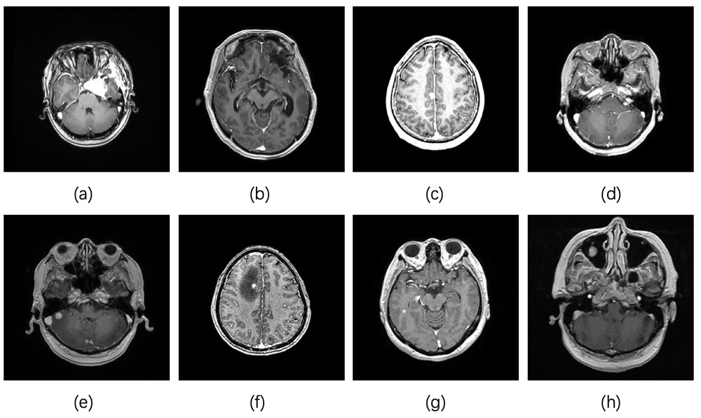
Figure 1: Sample from the used dataset. (a) Cavernous hemangioma, (b) Glioma, (c) Meningioma, (d) Acoustic neuroma, (e) Colorectal cancer brain metastasis, (f) Lung cancer brain metastasis, (g) Breast cancer brain metastasis, (h) No tumor.

III METHODOLOGY

We propose an experimental method for classifying the presence or absence of tumor and the source of tumor (primary or secondary intracranial tumor) based on brain MR images. The model is trained and optimized through the existing artificially annotated dataset to realize the classification of new images. In this section, the following sub-sections will introduce proposed methodology in detail.

III-A Proposed Method

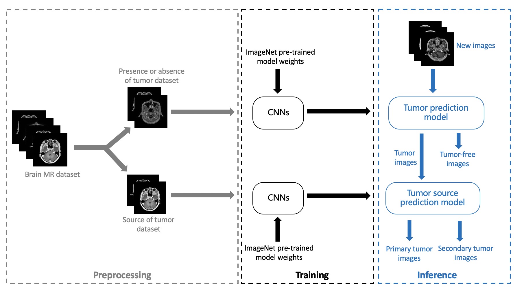
Figure 2: Flow chart of the proposed method.

Figure 2 shows the flow chart of the proposed method. First, the images in the brain MR dataset are selected into the presence or absence of tumor dataset and the tumor source type dataset according to tumor presence and source type labels. In the preprocessing stage, we use the bilinear interpolation method to unify the image size to 256×256. And we randomly flip 50% of the pictures horizontally. In this way, although the position of the pixels in the image is changed, the features are kept unchanged, which can enhance the generalization ability of the model. In the following CNN model, the values of pixels in the image will be converted into features. Therefore, the classification effect is dependent on these pixel values.We use normalization to limit the data to a certain range we need. This can prevent the unbalanced image pixel intensity distribution from interfering with subsequent processing. After preprocessing, we send the image to the model for traning. For large-scale network model with huge parameters, when performing medical tasks with relatively rare dataset, there is a certain gap in task performance between using pre-trained model and training from scratch [14]. We used the ImageNet pre-trained model based on pytorch. In each round of iterative training, the model parameters are automatically adjusted based on the prediction results of the previous round. The maximum number of training iterations is set to 100 epochs. We use SGD optimizer to update the weights of the network with a batch size of 16. And an initial learning rate of $\alpha_{0}$ at the very beginning and cosine decays are as following:

$$\alpha=\frac{1}{2}\times(1+cos(\frac{e\times\pi}{N_{e}}))\times\alpha 0$$ (1)

where $e$ is an epoch counter, and $N_{e}$ is a total number of epochs. The $\alpha_{0}$ for presence or absence of tumor model and source of tumor model are 1e-3 and 1e-4 respectively. After the two models are trained, the two optimized prediction models can be used to sequentially classify the presence or absence of tumors and the type of tumor source on the new image. The model is mounted on Huawei G5500 series servers and uses 1 NVIDIA V100 GPU card. The implementation of our network is based on PyTorch.

III-B Existing Classification Networks Comparison

We compare the effects of commonly used CNNs in recent years in the classification of tumor presence and source. 80% of brain MR dataset were used to train the model, and the remaining images were used to test the model. Finally, the testing accuracy is as shown in Figure 3.

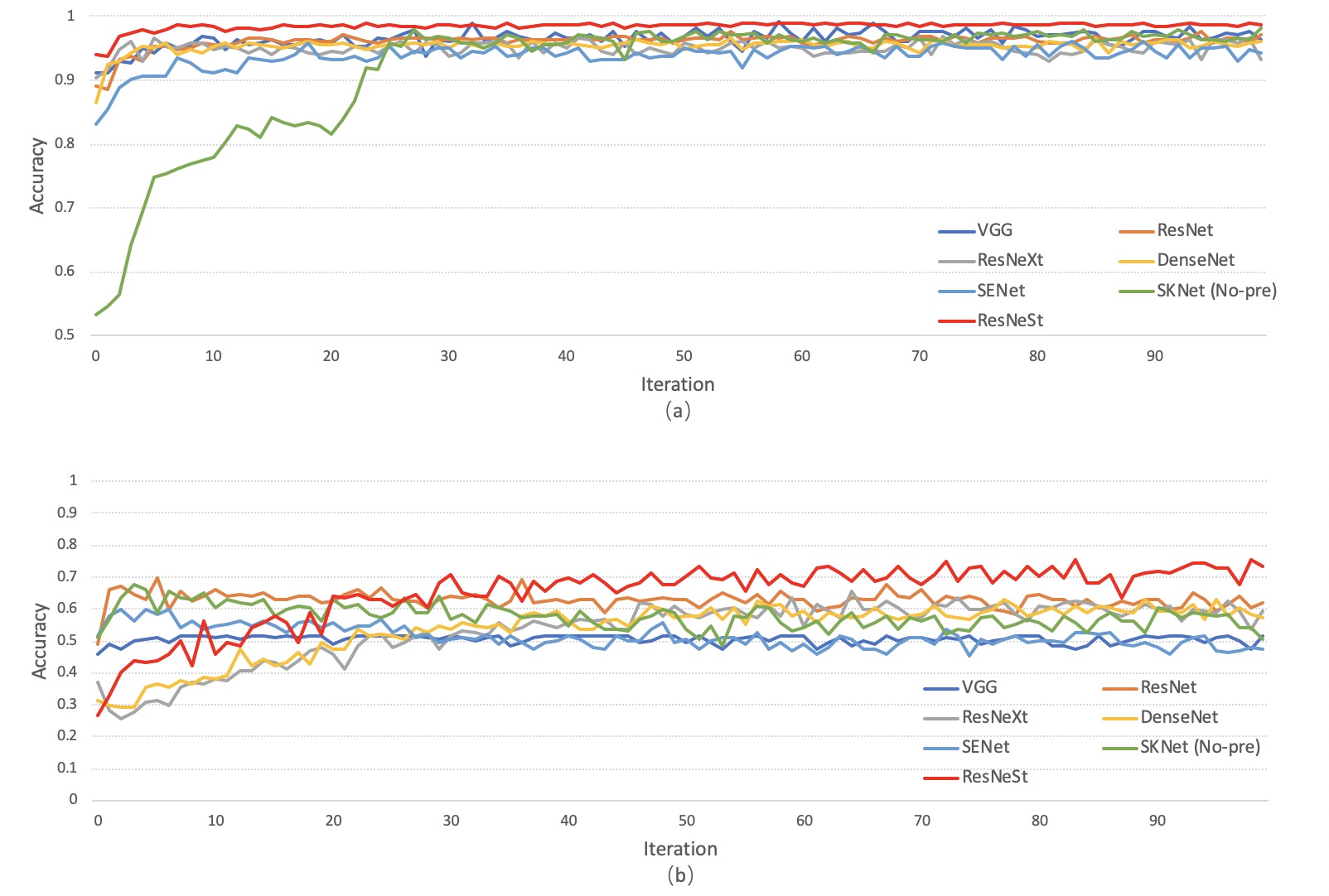
Figure 3: Baseline Comparison. (a) Presence or absence of tumor, (b) Source of tumor.

It can be seen that on the two classification tasks, the red line performs better. Especially in the classification task of tumor source type, most models cannot effectively distinguish the features between tumors from different sources, but ResNeSt performs well. Therefore, we decided to make the model architecture improvement based on this network to achieve a higher level of task performance.

III-C Proposed Architecture ResNeSAt

Our method is improved on ResNeSt [7]. We borrowed its split mechanism, so that multiple convolution kernel branches in the same layer can extract features separately, making the features more diverse. At the same time, our method uses the channel attention mechanism, which is achieved by assigning different weights to channels of different branches. Next, we use the spatial attention module (SA) in CBAM [9], so we call the proposed model ResNeSAt. SA generates a spatial attention map by concatenating the global pooling and maximum pooling and then convolving to extract the spatial relationship between the elements. In ResNeSAt, we inserted SA into each bottleneck in order to make the entire network pay more attention to the tumor area when extracting features, as shown in Figure 4. Where $\bigotimes$ and $\bigoplus$ represent element-wise multiplication and element-wise summation respectively.

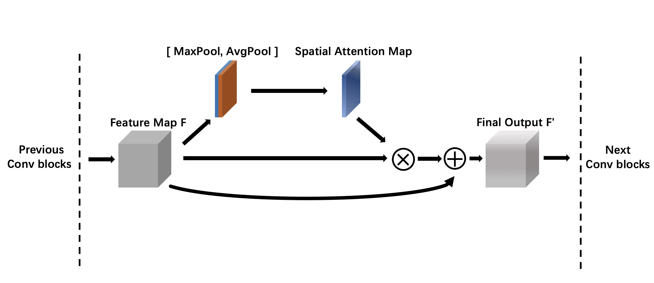
Figure 4: SA integrated with Bottleneck in ResNeSAt.

TABLE II: Details of network ResNeSAt.

ResNeSAt	Name	Details	Repeat
	Input
InitConv	InitConv 1	Conv3, BN, ReLU	2
	InitConv 2	Conv3, BN, ReLU, MaxPool	1
Layer 1	Bottleneck 1	Conv1, BN, SplAtConv, Conv1, BN, ReLU, SA, AvgPool, Conv1, BN	1
	Bottleneck 2	Conv1, BN, SplAtConv, Conv1, BN, ReLU, SA	2
Layer 2	Bottleneck 3	Conv1, BN, AvgPool, SplAtConv, Conv1, BN, ReLU, SA, AvgPool, Conv1, BN	1
	Bottleneck 4	Conv1, BN, SplAtConv, Conv1, BN, ReLU, SA	3
Layer 3	Bottleneck 5	Conv1, BN, AvgPool, SplAtConv, Conv1, BN, ReLU, SA, AvgPool, Conv1, BN	1
	Bottleneck 6	Conv1, BN, SplAtConv, Conv1, BN, ReLU, SA	5
Layer 4	Bottleneck 7	Conv1, BN, AvgPool, SplAtConv, Conv1, BN, ReLU, SA, AvgPool, Conv1, BN	1
	Bottleneck 8	Conv1, BN, SplAtConv, Conv1, BN, ReLU, SA	2
	Classifier	GlobalAvgPool, FC	1

III-D Performance Evaluation

We have evaluated the classification performance based on recall, specficity, precision, F1-score, and accuracy. To evaluate these metrics, we use four indices: Truly Positive (TP), False Positive (FP), False Negative (FN) and True Negative (TN) and define the following mathematical expressions.

$$Recall=\frac{TP}{TP+FN}$$ (2)

$$Specificity=\frac{TN}{TN+FP}$$ (3)

$$Precision=\frac{TP}{TP+FP}$$ (4)

$$F1-Score=2\times\frac{Recall\times Precision}{Recall+Precision}$$ (5)

$$Accuracy=\frac{TP+TN}{TP+TN+FP+FN}$$ (6)

Recall and Specificity describe how good the classifier is at classifying the positive and negative condition. Precision is the positive predictive rate. F1-score measure the classification performance in term of recall and precision. Accuracy is the overall classification accuracy of the proposed method.

IV EXPERIMENTAL RESULTS

The variability of a single model can be quite high. We evaluated the classification performance of the proposed model ResNeSAt and compared it with ResNeSt on ten-fold cross-validation and summarized our results in the form of tables. Table III and Table IV show the average recall, specificity, precision, F1-score and accuracy of best performed proposed CNN model on ten-fold testing datasets.

As shown in Table III, we can see that our proposed model ResNeSAt has improved recall, specificity,precision, F1-score and accuracy in classifying the presence or absence of tumor. This shows that ResNeSAt pays more attention to the tumor area, so it can better judge whether there is a tumor in the image. As shown in Table IV, in terms of judging the type of tumor source, we found that the improved model ResNeSAt has improved recall, F1-score, and accuracy. Specificity and precision can be almost ignored compared to the more comprehensive indicators F1-score and Accuracy. This shows that when judging the source type of the tumor, ResNeSAt better analyses the details of the tumor area and improves the classification performance to a certain extent. The parameter of the ResNeSt is 97.45 MB, and the parameter of the ResNeSAt is only 97.46 MB. In general, ResNeSAt effectively improves the accuracy of classification of tumor presence or absence and tumor source type, almost without increasing the model size.

TABLE III: Presence or absence of tumor model.

	Recall	Specificity	Precision	F1-score	Accuracy
ResNeSt	0.9733	0.9772	0.9803	0.9768	0.9751
ResNeSAt	0.9864	0.9981	0.9983	0.9923	0.9918

TABLE IV: Source of tumor model (primary or secondary).

	Recall	Specificity	Precision	F1-score	Accuracy
ResNeSt	0.7927	0.8684	0.8718	0.8304	0.8283
ResNeSAt	0.8212	0.8480	0.8591	0.8397	0.8338

V CONCLUSIONS & FUTURE WORK

In this paper, we use an attention guided deep learning method to solve the problem of tumor source classification, and further improve the effect of classifying the presence or absence of tumor. Using clinical case data generated by Shanghai Ruijin Hospital, we propose the ResNeSAt network for training and optimization, and classify the presence or absence of tumor and the type of tumor source on the tumor image within the error tolerance. This method produces a fast and accurate differential diagnosis with less subjective bias. It can reduce the dependence on experts in the clinical tumor image prediction process, and improve the efficiency and accuracy of diagnosis. Meanwhile, there is still room for improvement in the classification task of tumor source type. In future work, we can try segmentation of key areas to capture small differences between different images, which may aid to differentiate tumors classification further.

References

- [1] Simonyan K, Zisserman A. Very deep convolutional networks for large-scale image recognition[J]. arXiv preprint arXiv:1409.1556, 2014.
- [2] He K, Zhang X, Ren S, et al. Deep residual learning for image recognition[C]//Proceedings of the IEEE conference on computer vision and pattern recognition. 2016: 770-778.
- [3] Xie S, Girshick R, Dollár P, et al. Aggregated residual transformations for deep neural networks[C]//Proceedings of the IEEE conference on computer vision and pattern recognition. 2017: 1492-1500.
- [4] Huang G, Liu Z, Van Der Maaten L, et al. Densely connected convolutional networks[C]//Proceedings of the IEEE conference on computer vision and pattern recognition. 2017: 4700-4708.
- [5] Hu J, Shen L, Sun G. Squeeze-and-excitation networks[C]//Proceedings of the IEEE conference on computer vision and pattern recognition. 2018: 7132-7141.
- [6] Li X, Wang W, Hu X, et al. Selective kernel networks[C]//Proceedings of the IEEE conference on computer vision and pattern recognition. 2019: 510-519.
- [7] Zhang H, Wu C, Zhang Z, et al. Resnest: Split-attention networks[J]. arXiv preprint arXiv:2004.08955, 2020.
- [8] Yosinski J, Clune J, Bengio Y, et al. How transferable are features in deep neural networks?[C]//Advances in neural information processing systems. 2014: 3320-3328.
- [9] Woo S, Park J, Lee J Y, et al. Cbam: Convolutional block attention module[C]//Proceedings of the European conference on computer vision (ECCV). 2018: 3-19.
- [10] Muhammad K, Khan S, Del Ser J, et al. Deep learning for multigrade brain tumor classification in smart healthcare systems: A prospective survey[J]. IEEE Transactions on Neural Networks and Learning Systems, 2020.
- [11] Ge C, Qu Q, Gu I Y H, et al. 3D multi-scale convolutional networks for glioma grading using MR images[C]//2018 25th IEEE International Conference on Image Processing (ICIP). IEEE, 2018: 141-145.
- [12] Swati Z N K, Zhao Q, Kabir M, et al. Brain tumor classification for MR images using transfer learning and fine-tuning[J]. Computerized Medical Imaging and Graphics, 2019, 75: 34-46.
- [13] Zhang H, Mo J, Jiang H, et al. Deep Learning Model for the Automated Detection and Histopathological Prediction of Meningioma[J]. Neuroinformatics, 2020: 1-10.
- [14] Raghu M, Zhang C, Kleinberg J, et al. Transfusion: Understanding transfer learning for medical imaging[C]//Advances in neural information processing systems. 2019: 3347-3357.