Depth Completion with Twin Surface Extrapolation at Occlusion Boundaries

Abstract

Depth completion starts from a sparse set of known depth values and estimates the unknown depths for the remaining image pixels. Most methods model this as depth interpolation and erroneously interpolate depth pixels into the empty space between spatially distinct objects, resulting in depth-smearing across occlusion boundaries. Here we propose a multi-hypothesis depth representation that explicitly models both foreground and background depths in the difficult occlusion-boundary regions. Our method can be thought of as performing twin-surface extrapolation, rather than interpolation, in these regions. Next our method fuses these extrapolated surfaces into a single depth image leveraging the image data. Key to our method is the use of an asymmetric loss function that operates on a novel twin-surface representation. This enables us to train a network to simultaneously do surface extrapolation and surface fusion. We characterize our loss function and compare with other common losses. Finally, we validate our method on three different datasets; KITTI, an outdoor real-world dataset, NYU2, indoor real-world depth dataset and Virtual KITTI, a photo-realistic synthetic dataset with dense groundtruth, and demonstrate improvement over the state of the art.

1 Introduction

Depth completion problems involve estimating a dense depth image from sparse depth measurements of active depth sensors, often guided by a high-resolution modality; e.g., RGB sensors. Solving depth completion has extensive applications, e.g., scene understanding [24], object shape estimation [5], and $3$D object detection in autonomous driving [21].

Step-like object discontinuities are an inherent property of $3D$ scenes, and are challenging to model well with depth completion and depth super-resolution methods. It is important to maintain depth discontinuities to facilitate object shape and pose estimation. Most prior works rely on conventional regression losses for depth completion which, albeit promising results in depth accuracy, suffer from depth smearing and hence shape distortion of objects. While [12] tackles this depth mixing problem, it has high computational and memory demand for accommodating many channels at high resolution. Another interesting work [19] learns non-local spatial affinity with spatial propagation network to eliminate smearing, but suffers from significant inference times and poor generalization due to sparse patterns (See Tab. 6).

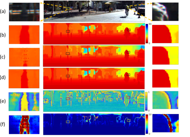
Figure 1: Our depth completion algorithm can input LiDAR data and image (a), and extrapolate the estimates of foreground depth $d_{1}$ (b) and background depth $d_{2}$ (c), along with a weight $\sigma$ (e). Fusing all three leads to the completed depth (d). The foreground-background depth difference (f) $d_{2}-d_{1}$ is small except at depth discontinuities.

One fundamental challenge of recovering depth discontinuity is that pixels at boundary regions suffer from ambiguity as to whether they belong to a foreground depth or background depth. Some methods seek to reduce the impact of ambiguities through intelligent regularization of the loss function [10] or ranking loss [33] at potential occlusion boundaries; and others explicitly train detectors for depth discontinuities [11] via full dense ground truth data. Unfortunately large scale datasets like KITTI have only partial dense ground truth depth (see Fig. 2 (a)) which is sparse on boundaries, making it difficult to explicitly label occlusion boundaries. Some recent works have leveraged prior information, e.g., estimated semantic maps [40, 7, 32] and estimated depth maps [23] for object boundary recovery/refinement. Our approach instead seeks to explicitly model ambiguity and leverage it in depth completion. We noted that Depth coefficients [12] can also model ambiguities on account of its non-parametric probability distribution, but maintaining many high-resolution channels is computationally and memory expensive, and also suffer from the binning resolution. Instead of using multiple channels with binning, our method, named TWIn-Surface Estimation (TWISE), uses a two-surface representation which is much more efficient and can explicitly model ambiguity by finding difference between the twin surface depths. We believe that naturally encoding the foreground and background pixels at the boundary would enable the effective learning of the step-wise discontinuity with lower memory and computational requirement.

In order to train a twin-surface estimator, we propose a pair of asymmetric loss functions that naturally bias estimates toward foreground and background depth surfaces. The asymmetry in the losses are key to separation of foreground and background depths at ambiguous pixels. We also incorporate a fusion channel that automatically combines the foreground and background depths into a final depth estimate for each pixel, by selecting a foreground/background depth at the ambiguous regions and mixing the two depths at non-ambiguous regions.

Of particular concern is the lack of dense and reliable ground-truth depth data in outdoor scenes needed for accurate evaluation of depth estimates. KITTI, a realistic outdoor scene dataset, offers semi-dense ground-truth, created by accumulating LiDAR points but suffers from noisy depth samples (outliers) at boundaries and dynamic objects [30]. Indoor dataset like NYU2 provides dense GT only by using some colorization techniques that can cause smoothing at object boundaries. Currently the preferred evaluation metric of choice for ranking depth completion methods is RMSE. In this paper, we study the effects of outlier noise present in ground-truth data on RMSE and note that MAE is a more consistent metric for both cases of noisy and clean ground-truth, as validated on the synthetic VKITTI dataset.

The contributions of this paper are as follows:

• We propose a twin-surface representation that can estimate foreground, background and fused depth.

• We adopt a pair of assymmetric loss functions to explicitly predict foreground-background object surfaces.

• We validate our theory in KITTI, a challenging outdoor scene dataset for depth completion, and show the superiority of our method on several metrics, and also show it generalizes well to variable sparsity and offers competitive inference times over the SoTA.

• We suggest that in presence of outliers, MAE is a more consistent metric to rank methods compared to RMSE, and we validate this claim with extensive experiments in VKITTI, a synthetic dataset for urban driving scenario.

2 Related Works

Depth Completion

Deep neural networks (DNNs) have been applied to the depth completion problem, in works such as Sparse-to-Dense [16], DDP [38], and Spade RGBsD [13]. These works show that by using standard encoder-decoder architecture (ResNet and MobileNet), it is possible to improve depth estimation accuracy via regression losses like $L_{2}$, $L_{1}$ and inverse $L_{1}$ losses. Deep-Lidar [22] estimates surface normal and dense depth using multiple DNNs to assist in further fine-tuning dense depth. Both [22] and [38] rely on synthetic data and various labels for learning depth representations. Recently, works have opted to optimize depth using $3$D geometric constraints like depth-normal consistency [39, 36] to improve depth completion. Xu et al. create geometric consistency between the surface normal and depth in $3$D, but use another refinement network for improved depth estimation [36]. Another recent trend is to learn spatial propagation of pixels in $2$D depth space for depth completion problems in fixed [4] or variable receptive field [19, 37]. Although results are highly encouraging, these methods suffer from poor inference times and generalizability on variable sparsity. Researchers have also looked into learning $3$D features for depth completion using continuous convolution in $3$D space [2], point cloud completion [34], $3$D graph neural networks [35] for dynamic construction of local neighborhood regions.

Depth Representations

Depth maps, as $2.5$D representations, have been used for RGBD fusion and instance segmentation [26, 8]. They naturally encode sensor viewing rays and adjacency between points. They are compact representations and their regular grids can be processed with CNNs in an analogous way to image super-resolution [27, 28]. This is the representation of choice for colorization techniques and fusion [18] as well as depth completion.

We propose a $2$-layered representation of depth to model occlusion boundaries. The concept of layered representation of depth has been well known in graphics community. LDIs (Layered Depth Images) are first proposed by Shade et al. [25] as intermediate representation for efficient image-based rendering. These are gathered by accumulating depth values via z-buffering from multiple depth images of nearby view points. Tulsiani et al. [29] infer $2$-layered depth representation (recovering depth of visible and non-visible scene) from a single input image by learning view-synthesis from multiview camera guided supervision. Hedman et al. [9] propose a $3$D photo reconstruction algorithm that builds multi-layered geometric representation of the scene by warping several depth maps and stitching color and depth panoramas for front and back-scene surfaces. In all these cases, multi-layered representation is constructed/learned from multi-camera viewpoints/depthmaps of the scene. In our case, we estimate these $2$-layered representation on a single camera viewpoint with our proposed loss functions.

Loss Functions in Depth Completion

A key component of depth completion is the choice of loss functions. Recent work has explored loss functions including $L_{2}$ [3, 16], $L_{1}$ [17], inverse-$L_{1}$ [13], Huber loss [2] and Softmax loss on depth [15]. Another elegant way is to use combination of $L_{1}$ + $L_{2}$ [19], which can leverage the benefits of both $L_{1}$ and $L_{2}$ losses. While these loss functions can achieve low error on metrics including RMSE, MAE, iMAE, often it comes at the cost of smoothing depth estimates across object boundaries. In addition to the aforementioned losses, people increasingly use Chamfer distance on point cloud [34], depth-normal constraint [36], Cosine loss [22], in a multi-learning framework to improve depth completion accuracy. Nevertheless, smoothing across sharp boundaries remains a concern in many of these methods. Imran et al. [12] show that cross-entropy (CE) loss can generate sharp boundaries, although performs worse in the RMSE metric.

We learn foreground and background depth by proposing two assymetric loss functions, and the final depth using a fusion loss. The assymetric loss function has been used in Vogel et al. [31], for the different purpose of denoising input images. We propose to use assymetric loss functions to learn biased estimators of FG/BG surface, and learn to select/blend (fusion loss) between FG/BG surface, and that, we claim, helps to recover depth discontinuity.

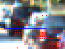
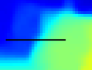
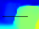
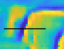
(a)	(b)	(c)	(d)
	(e)	(f)	(g)

Figure 2: Depth smearing across boundaries. We show the ground truth depth (colored red) overlaid on an image (a), depths estimated by the SoTA method [14] (b), our fused depths (c), our estimated weights $\sigma$ (d), a depth slice of [14] (e), fused depth and $\sigma$ slices (f), and foreground and background slice (g). Our extrapolation ability in (g) results in the sharp depth boundary in (f), rather than the smeared depth in (e).

3 Methodology

Depth completion involves two quite different challenges which can be at odds. The first is to interpolate missing pixel depths within objects leveraging nearby sparse depths. The second is to accurately find the occlusion boundaries of objects and ensure that interpolated pixels belong to either the foreground or background object. We propose a method that aims to perform both tasks well.

Our approach divides depth completion into two simpler problems, each of which can be more easily learned by a network. The first problem is depth interpolation without boundary determination. Rather than estimating a single surface which must model step functions at depth discontinuities, Our key novelty is to estimate twin surfaces. A foreground surface extrapolates the foreground object depth up to and beyond boundaries, while a background surface extrapolates the background depth up to and behind the occluding object. Then the second problem is to find the boundary and determine a single depth by fusing these two surfaces. We find the color image is particularly useful in aiding surface fusion. Both of these components are illustrated in Fig. 2.

3.1 Ambiguities and Expected Loss

Ambiguities have a significant impact on depth completion, and it is useful to have a quantitative way to assess their impact. Here we propose using the expected loss to predict and explain the impact of ambiguities on trained networks.

By an ambiguity we mean, not that there isn’t a unique true solution, but rather that from a measurement it is difficult for the algorithm and/or human to decide between two or more distinct solutions. Ambiguity can be more formally defined as follows. Given measurement data that sparsely samples the scene, the number of ambiguities is equal to the number of different true scenes, i.e. true depth maps in our case, that could have generated the sparse measurement. This number depends on what variations occur in actual data. For simplicity we treat each pixel ambiguity independently of other pixels, and so the ambiguities for a pixel are the possible depth values it could take that are consistent with the measurement.

We anticipate the level of ambiguity to vary across a scene. For example, pixels on flat surfaces will be well-constrained by nearby pixels and have low ambiguity. In contrast, pixels near depth discontinuities may have large depth ambiguity. There is often insufficient data from the depth image to decide whether the pixel is on the foreground or background.

A corresponding color image can help resolve ambiguities as to which object a pixel belongs. However, exactly how to leverage color images to resolve ambiguities in CNNs is one of the open challenges in depth completion. Our work aims to offer a solution to this problem by explicitly estimating ambiguities and resolving them within the network.

To assess the impact of ambiguities on our network, we build a quantitative model. Consider a single pixel whose depth, $d$, we seek to estimate. Next assume that the pixel has a set of ambiguities, $d_{i}$, each with probability $p_{i}$. This probability measures of how likely it is that the ground truth will take the corresponding depth, given our modeled scene assumptions. Now consider a loss function on the error for each pixel, $L(d-d_{t})$, where $d_{t}$ is the ground truth depth. The expected loss as a function of depth is:

$$E\{L(d)\}=\sum_{i}p_{i}L(d-d_{i}).$$ (1)

This expected loss is important because if a network is trained on representative data then it will be trained to minimize the expected loss. Thus by examining the expected loss we can predict the behavior of our network at ambiguities, and so justify the design of our method.

3.2 Asymmetric Linear Error

Our method uses a pair of error functions which we call the Asymmetric Linear Error (ALE), and its twin, the Reflected Asymmetric Linear Error (RALE), defined as:

$$ALE_{\gamma}\left(\varepsilon\right)=\mbox{max}\left(-\frac{1}{\gamma}\varepsilon,\gamma\varepsilon\right),$$ (2)

$$RALE_{\gamma}\left(\varepsilon\right)=\mbox{max}\left(\frac{1}{\gamma}\varepsilon,-\gamma\varepsilon\right).$$ (3)

Here $\varepsilon$ is the difference between the measurement and the ground truth, $\gamma$ is a parameter, and $\mbox{max}(a,b)$ returns the larger of $a$ and $b$. The ALE and RALE are generalizations of the absolute error, and are identical to the absolute error when $\gamma=1$. The difference is that the negative side of ALE is weighted by $\nicefrac{{1}}{{\gamma}}$ and the positive weighted by $\gamma$. The RALE is simply the reflection of the ALE over the $\varepsilon=0$ line. Both are illustrated in Fig. 3 (a,b).

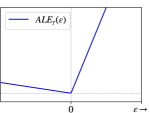
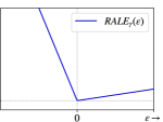
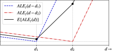
(a)	(b)	(c)

Figure 3: (a) The ALE from Eq. (2) is asymmetric around its minimum at the origin. (b) The RALE from Eq. (3) is a reflection of the ALE. We use the ALE for foreground surface estimation and the RALE for background estimation. (c) A pixel depth is shown with two ambiguities at depths $d_{1}$ and $d_{2}$ and probabilities $p1$ and $p1$ respectively. The black line shows the expected ALE which is the probability-weighted sum of two ALE functions, see Eq. (1). The expected ALE will have a minimum at one of the marked corners occurring at $d_{1}$ and $d_{2}$. The minimum will be at $d_{1}$ if Eq. (4) is satisfied, as it is in this case with $p_{1}=p_{2}$, and so acts as a foreground depth estimator.

Note that if $\gamma$ is replaced by $\nicefrac{{1}}{{\gamma}}$, both the ALE and RALE are reflected. Thus, without loss of generality, in this work we restrict $\gamma\geq 1$.

3.3 Foreground and Background Estimators

We make a further simplifying assumption in our analysis that there are at most binary ambiguities per pixel. A binary ambiguity is described by a pixel having probabilities $p_{1}$ and $p_{2}$ of depths $d_{1}$ and $d_{2}$ respectively. When $d_{1}<d_{2}$ we call $d_{1}$ the foreground depth and $d_{2}$ the background depth. Such a binary ambiguity is likely to occur near object-boundary depth discontinuities.

To estimate the foreground depth we propose minimizing the mean ALE over all pixels to obtain $\hat{d}_{1}$, the estimated foreground surface. To predict the characteristics of $\hat{d}_{1}$ from a trained network at ambiguous pixels, we examine the expected ALE, as shown in Fig. 3 (c). This is piecewise linear and has two corners, one at $d_{1}$ and the other at $d_{2}$. The lower of these will determine the minimum expected loss, and hence what an ideal network will predict. Using Eqs. (2) and (1), we obtain expected losses: $L(d_{1})=p_{2}(d_{2}-d_{1})/\gamma$, and $L(d_{2})=p_{1}(d_{2}-d_{1})\gamma$. From this it is straightforward to see $L(d_{1})<L(d_{2})$ when:

$$\gamma>\sqrt{\frac{p_{2}}{p_{1}}}.$$ (4)

This equation shows the sensitivity of the foreground estimator to $\gamma$; the higher $\gamma$, the lower the probability on foreground $p_{1}$ needed for the minimum to be at the foreground depth $d_{1}$.

To estimate the background depth, $\hat{d}_{2}$, at boundaries we propose minimizing the expected RALE. The same analysis will apply to this as to the ALE, and we obtain the same constraint on $\gamma$ as in Eq. (4), except that the probability ratio is inverted.

Fig. 1 (b) shows an example foreground depth estimate, (c) the background depth and (f) the depth difference. We observe that at pixels far from depth discontinuities, as well as the sparse input-depth pixels, the foreground depth is very close to the background depth indicating no ambiguity.

3.4 Fused Depth Estimator

We desire to have a fused depth predictor that can do both interpolation and extrapolation at surfaces depending on ambiguous and non-ambiguous regions. The foreground and background depth estimates provide lower and upper bounds on the depth for each pixel. We express the final fused depth estimator $\hat{d}_{t}$ for the true depth $d_{t}$ as a weighted combination of the two depths:

$$\hat{d}_{t}=\sigma\hat{d}_{1}+(1-\sigma)\hat{d}_{2}.$$ (5)

where $\sigma$ is an estimated value between $0$ and $1$. We use a mean absolute error as part of the fusion loss:

$$F(\sigma)=|\hat{d}_{t}-d_{t}|=|\sigma\hat{d}_{1}+(1-\sigma)\hat{d}_{2}-d_{t}|.$$ (6)

The expected loss for this is

$$\begin{split}L_{e}(\sigma)=&E\{F(\sigma)\}=p|\sigma\hat{d}_{1}+(1-\sigma)\hat{d}_{2}-d_{1}|+\\ &(1-p)|\sigma\hat{d}_{1}+(1-\sigma)\hat{d}_{2}-d_{2}|.\end{split}$$ (7)

Here, $p$ = $p_{1}$, and $p_{2}$ = $1-p$. This has a minimum at $\sigma=1$ when $p>0.5$ and a minimum at $\sigma=0$ when $p<0.5$. Of course this assumes that depth is either $d_{1}$ or $d_{2}$.

Depth fusion occurs by optimizing the loss of Eq. (7) to predict a separate $\sigma$ for each pixel. In this way our fusion step is an explicit determination of whether a pixel is foreground or background or a combination. An example estimated $\sigma$ is shown in Fig. 1 (e).

3.5 Depth Surface Representation

We have developed three separate loss functions whose individual optimizations give us three separate components of a final depth estimate for each pixel. Based on the characterization of our losses, we require a network to produce a $3$-channel output. Then for simplicity we combine all loss functions into a single loss:

$${\vspace{-2mm}}\begin{split}L(c_{1},c_{2},c_{3})=&\frac{1}{N}\sum_{j}^{N}(ALE_{\gamma}\left(c_{1j}\right)+RALE_{\gamma}\left(c_{2j}\right)\\ &+F(s(c_{3j}))).\end{split}$$ (8)

Here $c_{ij}$ refers to pixel $j$ of channel $i$, $s()$ is a Sigmoid function, and the mean is taken over all $N$ pixels. We interpret the output of these three channels for a trained network as $c_{1}\rightarrow\hat{d}_{1}$, $c_{2}\rightarrow\hat{d}_{2}$ and $s(c_{3})\rightarrow\sigma$, and combine them as in Eq. (5) to obtain a depth estimator $\hat{d}_{t}$ for each pixel.

3.6 Implementation Details

Architecture

This work presents novel loss functions linked to a multi-channel depth representation. These can be easily incorporated into a variety of network architectures with minimal change to the network. Specifically we selected the multistack network [14], with the author-provided code. We choose this network due to its fast inference time, lower number of parameters than [16], and its near-SoTA performance. The changes we made were three output channels and instead of one at each stacked hourglass network, and we use our loss function for the optimization. We used $64$ channels in the encoder-decoder network as that provided their highest performing results. More details are shared in the supplementary material.

Training and Inference

We followed the training protocol in [14] with multi-scale supervision on our $3$ channels. The total loss is a weighted sum of the multiple resolution losses $L_{i}$, where $L_{1}$ is the full resolution $3$-channel loss in Eq. (8), $L_{2}$ is half-resolution and $L_{3}$ quarter resolution: $L=\omega_{1}L_{1}+\omega_{2}L_{2}+\omega_{3}L_{3}$. The multiscale stage training protocol sets $\omega_{1}=\omega_{2}=\omega_{3}=1$ during the first $10$ epochs, reduces $\omega_{2}=\omega_{3}=0.1$, and continues to train for another $10$ epochs. For the last $10$ epochs we set $\omega_{2}=\omega_{3}=0$ and complete training after $30$ epochs. Using Adam optimizer with an initial learning rate of $10e-3$ and decrease to half every $5$ epochs, we train a full sized image with gradient accumulated every $4$ samples in a batch. We use PyTorch [20] for our implementation.

Method	MAE	RMSE	iMAE	iRMSE	TMAE [12]	TRMSE [12]	Infer. time (sec.)
Ma et al. [16]	$249.95$/$269.2$	$814.73$/$878.5$	$1.21$/$1.34$	$2.80$/$3.25$	–/$190.15$	–/$297.48$	$0.081$
Depth-Normal [36]	$235.17/236.67$	$777.05/811.07$	$1.79/1.11$	$2.42/2.45$	–/–	–/–	–
DeepLidar [22]	$226.50$/$215.38$	$758.40$/$687.0$	$1.15$/$1.10$	$2.56$/$2.51$	–/$162.75$	–/$266.79$	$0.097$
3DepthNet [34]	$226.2$/$208.96$	$798.40$/$693.23$	$1.02$/$0.98$	$2.36$/$2.37$	–/–	–/–	–
Uber-FuseNet [2]	$221.19$/$217.0$	$752.88$/$785.0$	$1.14$/$1.08$	$2.34$/$2.36$	–/–	–/–	–
MultiStack [14]	$220.41$/$223.40$	$762.20$/$798.80$	$0.98$/$1.0$	$2.30$/$2.57$	–/$157.90$	–/$270.15$	$0.018$
DC-3co [12]	$215.75$/$215.04$	$965.87$/$1011.3$	$0.98$/$0.94$	$2.43$/$2.50$	–/$141.67$	–/$238.5$	$0.112$
CSPN++ [4]	$209.28$/–	$743.69$/–	$0.90$/–	$2.07$/–	–/–	–/–	$0.200$
DDP [38]	$205.40$/–	$836.00$/–	$0.86$/–	$2.12$/–	–/–	–/–	–
NLSPN [19]	$199.59/198.64$	$\bm{741.68}/771.8$	$0.84/0.83$	$1.99$/$2.03$	–/$138.81$	–/$248.88$	$0.225$
TWISE	$195.58$/$193.40$	$840.20$/$879.40$	$0.82$/$0.81$	$2.08$/$2.19$	–/$131.60$	–/$239.80$	$0.022$

Table 1: Depth completion on the Test/Validation sets of KITTI, with $64$R LiDAR and RGB input (units in mm).

[]
[]
[]
[]
[]

Figure 4: Comparison of our method with SoTA methods with whole and zoom in views (a) showing Color Images (b) DC [12], (c) MultiStack [14] (d) NLSPN [19] and our method (e). Four different regions of the image from two different instants are selected to show depth quality from diverse areas.

4 Experimental Results

Dataset

We evaluate the proposed algorithm on the standard KITTI Depth Completion dataset [6], a real-world outdoor scene, NYU2, with indoor scenes [18], and Virtual KITTI [1], a synthetic dataset with photo-realistic images and dense ground-truth depth. KITTI depth is created by aggregating LiDAR scans from $11$ consecutive frames into one, producing a semi-dense ground truth (GT) with $30$% annotated depth pixels. The sparsity of GT makes depth estimation more challenging. Note that we do not require any synthetic depth data for pre-training as used by [38, 22] to improve performance. The dataset consists of $85$K, $1$K, and $1$K samples for training, validation, and testing respectively. Although the training set has different image sizes, the test and validation sets are cropped to a uniform size of $352\times 1,216$.

Although created in a real world scenario, the semi-dense GT produced by Uhrig et al. [30] has far fewer depth points on object boundaries (see Fig. 2 (a)), and is susceptible to outliers. As we claim our method works well on boundaries, we also evaluate on VKITTI 2.0, a synthetic dataset with clean and dense GT depth at depth discontinuities. The VKITTI $2.0$, created by the Unity game engine, contains $5$ different camera locations ($15^{o}$ left, $15^{o}$ right, $30^{o}$ left, $30^{o}$ right, clone) in addition to $5$ different driving sequences. Additionally, there are stereo image pairs for each camera location. For training and testing, we only use the clone (forward facing camera) with stereo image pairs. For VKITTI training, $2$k training images were created from driving sequences $01$, $02$, $06$, and $018$ respectively. For testing, we use sequence $020$ at the left stereo camera, and choose every other frames, with total $420$ images. We subsample the dense GT depth in azimuth-elevation space to simulate LiDAR-like pattern as sparse inputs. Further, we create the pseudo GT following [30] to study the effects of outlier noise on training and evaluation. More details are shared in the supplementary.

To show the generalizibility of our method, we also evaluate on NYU-Depth v2 dataset [18], which consists of RGB and depth images obtained from Kinect in $464$ scenes. We use the official split of data, where $249$ scenes are used for training and we sample $50$K images out of the training similar to [22, 19]. For testing, the standard labelled set of $654$ images is used. The original image size is first downsampled to half, and then center-cropped, producing a network input dimension of $304\times 208$. Unlike [19], we use the same loss function for all the datasets.

Metrics

The standard metrics used by KITTI include RMSE, MAE, iMAE and iRMSE. Since RMSE is used as the preferred metric for depth completion, most SoTA methods on the KITTI leaderboard use MSE as their primary loss. We also include tMAE and tRMSE metrics proposed in [12] since it can discount outlier depth pixels (i.e., floating depth pixels around boundary regions) and give a better evaluation of depth pixels at and within object boundaries.

4.1 Results

Quantitative Results

Tab. 1 compares the performance on KITTI’s test/validation sets, with a $64$-row LiDAR and color image as input. We list the SoTA methods with performance quoted from their papers. The inference times are calculated on a single GPU of GTX $1080$ Ti. The method [19] with lowest RMSE achieves this at the expense of inference time. We outperform the SoTA methods in other metrics including MAE, and iMAE. The exception is RMSE, by which the methods are ranked in the KITTI leaderboard. That leads us to investigate in which areas are our method perform better and worse, which we examine next.

Qualitative Results

Fig. 4 shows our depth estimation quality compared to baselines. We choose three best SoTA methods: MultiStack [14], NLSPN [19], and DC [12]. Different local regions including poles, trees, cars, and traffic signs, illustrate the depth quality of close- and long-range depth pixels. The zoomed-in view shows the substantial improvement of our depth map over SoTA, especially along sharp object boundaries. [14] has a more blurred estimation around boundaries leading to mixed depth pixels and holes within objects, such as on the traffic poles and van. Although [19] has reduced mixed depths and more tighter boundary, depth mixing still exists (blurriness at object boundaries), additionally it suffers from jagged boundary edges and streaking artifacts.

[]

[] 

[]

[]

[]

[] 

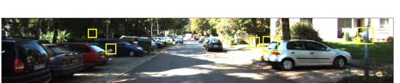
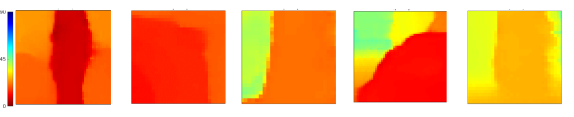
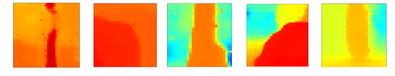
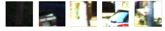
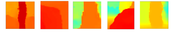
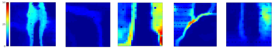
Figure 5: Input image (a), its zoom-in views (d), our estimation on foreground depth (b), background depth (c), fused depth (e), and the depth difference between foreground and background depth (f).

Qualitative Parsing

Fig. 5 offers a more detailed analysis of our method by showing different estimation at foreground, background depths and fused depth respectively. We choose five zoom-in views from diverse objects, e.g., tree, poles, car, and even pixels at far-away depth pixels. It shows that our fused depth estimator can learn to choose foreground and background regions well, resulting in a clear shape estimation of objects. We note that it is biased to choose the foreground surface as ambiguity increases, e.g., relatively large depth gap between foreground and background surfaces (see depth difference in Fig. 5 (f)). This can be explained by the fact that there are more supervision at the close-up region than the far-away region on account of uneven distribution of GT depth pixels.

Quantitative Results on NYU2

: Results on NYU2 are shown in Tab. 2, based on its standard metrics. We are currently ranked the second in all standard metrics. Note that compared to NLSPN [19], ours is $10\times$ faster in inference on KITTI. The results also show that TWISE is equally generalizable to indoor scenes.

Method	RMSE (m)	REL	$\delta_{1.25}$	$\delta_{1.25}^{2}$	$\delta_{1.25}^{3}$
DC-3co [12]	$0.118$	$0.013$	$99.4$	$99.9$	$100.0$
DeepLidar [22]	$0.115$	$0.022$	$99.3$	$99.9$	$100.0$
DepthNormal [36]	$0.112$	$0.018$	$99.5$	$99.9$	$100.0$
GNN [35]	$0.106$	$0.016$	$99.6$	$99.9$	$100.0$
TWISE	$0.097$	$0.013$	$99.6$	$99.9$	$100.0$
NLSPN [19]	$0.092$	$0.012$	$99.6$	$99.9$	$100.0$

Table 2: Depth completion results on NYU2 [18].

4.2 Ablation Studies

In this section, we conduct extensive ablation studies to investigate the effect of different parameters of our proposed loss. We train with $1/6$ data ($\sim$$12$K training samples) due to resource constraints, and maintain this protocol for all ablations unless otherwise noted.

Effect of Loss Functions

We show that performance of our loss function is network agnostic. Tab. 3 refers to different loss functions typically used in SoTA depth estimation works. Although $L_{2}$ is a widely used loss for estimating depth [16, 14, 3], $L_{1}$ loss [17], Huber loss [2], $L_{1}+L_{2}$ [19] are some of the widely used losses for depth completion. We compare our TWISE loss with all others, including the CE loss [12]. Top performances on MAE and TMAE show the positive side effect of our loss addressing the smearing problem at the boundary. We particularly note that TWISE performs better than a standard $L_{1}$ loss on both the backbone networks, leading to believe that TWISE offers more benefit than a mere trade-off between MAE and RMSE.

	Res-18 [16]				MultiStack [14]
Loss	MAE	RMSE	TMAE	TRMSE	MAE	RMSE	TMAE	TRMSE
$L_{1}$ [17]	$282.6$	$110.6$	$181.8$	$295.6$	$211.0$	$950.0$	$138.6$	$246.0$
$L_{2}$ [16]	$341.2$	$987.8$	$244.6$	$349.5$	$247.4$	$880.0$	$170.3$	$285.0$
$L_{2}$+$L_{1}$ [19]	$298.8$	$972.2$	$206.5$	$316.7$	$231.8$	$\bm{887.5}$	$156.9$	$271.2$
Huber [2]	$288.6$	$1039.6$	$198.0$	$302.1$	$222.6$	$927.1$	$153.9$	$256.0$
CE [12]	$279.1$	$1125.1$	$184.3$	$239.1$	–	–	–	–
TWISE	$275.5$	$1045.1$	$181.1$	$294.0$	$201.3$	$927.6$	$134.1$	$240.1$

Table 3: Effect of different loss functions. Compared to single channel losses, CE requires $80$ channel, while TWISE requires 3 channel.

Options	MAE	RMSE	TMAE	TRMSE
$\hat{d_{t}}=\hat{d_{1}}$ ($\sigma=1$)	$306.9$	$1109.9$	$204.4$	$314.8$
$\hat{d_{t}}=\hat{d_{2}}$ ($\sigma=0$)	$295.4$	$1092.9$	$193.9$	$306.1$
$\hat{d_{t}}=0.5*(\hat{d_{1}}+\hat{d_{2}})$ ($\sigma=0.5$)	$220.7$	$854.8$	$148.2$	$262.4$
$\hat{d_{t}}=\hat{d_{1}}/\hat{d_{2}}|\sigma>0.5$	$261.0$	$1008.0$	$180.4$	$287.9$
No color	$222.4$	$1067.5$	$139.2$	$247.8$
$\hat{d_{t}}=\sigma\hat{d_{1}}+(1-\sigma)\hat{d_{2}}$	$193.4$	$879.4$	$131.1$	$236.0$

Table 4: Effect of learned $\sigma$ in TWISE, evaluated by our best model.

$\gamma$	MAE	RMSE	TMAE	TRMSE
$1.0$	$223.1$	$950.1$	$145.8$	$257.0$
$1.5$	$207.8$	$947.9$	$138.1$	$245.1$
$2.0$	$201.3$	$927.6$	$134.1$	$240.1$
$2.5$	$204.4$	$932.5$	$136.1$	$242.5$
$5.0$	$207.1$	$923.4$	$138.7$	$246.1$
$10$	$216.1$	$922.8$	$146.7$	$255.4$

Table 5: Effect of $\gamma$ on depth completion performance.

Supervision		Noisy Semi-Dense GT				Clean GT
Backbone	Method	MAE	RMSE	TMAE	TRMSE	MAE	RMSE	TMAE	TRMSE
MultiStack [14]	$L_{1}$	$8.79$	$49.9$	$7.09$	$16.02$	$14.43$	$130.62$	$6.16$	$18.28$
	$L_{2}$	$10.40$	$45.35$	$8.61$	$17.89$	$17.75$	$127.14$	$8.45$	$20.18$
	$L_{1}+L_{2}$	$9.42$	$44.90$	$8.23$	$16.82$	$15.45$	$126.20$	$7.14$	$19.30$
	TWISE	$7.98$	$47.5$	$6.25$	$15.35$	$12.71$	$126.4$	$5.22$	$16.67$
ResNet-18 [16]	CE	$10.50$	$58.67$	$8.64$	$16.57$	$19.03$	$155.24$	$8.26$	$18.29$
	$L_{1}$	$12.95$	$62.97$	$14.68$	$19.25$	$23.52$	$147.42$	$12.51$	$29.33$
	$L_{2}$	$17.45$	$50.48$	$17.48$	$21.26$	$27.48$	$133.21$	$15.57$	$36.73$
	$L_{1}+L_{2}$	$14.21$	$48.25$	$15.80$	$20.10$	$25.40$	$132.6$	$14.35$	$32.47$
	TWISE	$10.24$	$52.37$	$8.42$	$16.77$	$18.88$	$132.94$	$9.45$	$18.17$

Figure 6:                                                (a)

                         

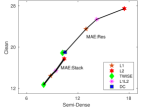
Figure 7:                                                      (b)

     

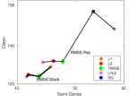
Figure 8:              (c)

Figure 9: (a) Results on Virtual KITTI experiments trained on clean GT and synthesized semi-dense respectively (units in cm). (b) MAE and (c) RMSE curves of scatter plots (Semi-Dense vs Clean GT) for different loss functions (colored symbols) and two backbone networks (MultiStack [14] and ResNet-18 [16]). Methods trained with the same backbone network are connected.

Effect of $\sigma$ on Estimated Surfaces

Another interesting evaluation is the importance of learned $\sigma$ on different estimated surfaces. In Tab. 4, we evaluate estimated depths for different combinations of $\sigma$ and compare individually its depth completion metrics. The performance is evaluated on our best model in Tab. 1, except for the row with “no color”, where we train without color input on the same network of our best model. From Tab. 4, foreground and background depth surface estimates, as usual, have higher error metric, since they are individually a biased estimate of depth. If we fix $\sigma$ at $0.5$, we see it is possible to achieve decent performance on MAE and RMSE on account of averaging (interpolation) between the two surfaces. We make a binary choice between foreground and background surface if $\sigma>0.5$ and the results are worse than averaging. In addition, we see $\sigma$ does not learn effectively without color input. So high-resolution imagery helps to learn effective $\sigma$ and resolve ambiguities at the boundaries.

Effect of $\gamma$ on Performance

Since $\gamma$ impacts the separation of foreground and background surfaces, we perform an ablation to assess its impact on TWISE. Tab. 5 shows depth completion performance with several $\gamma$ values. With $\gamma=1$, the loss is equivalent to MAE. As $\gamma$ increases, the gap between foreground and background surface increases. At small $\gamma$ values, the interpolation benefits, thus leading to lower MAE, TMAE, TRMSE, since it is easier to interpolate between two nearby surfaces; however, in the meantime extrapolation suffers, thus leading to higher RMSE. At larger $\gamma$, the slope between two surfaces increase, and interpolation becomes harder. We choose $\gamma=2.0$ in our experiment as a compromise between interpolation and extrapolation.

Effect of Sparsity on Depth Performance

We also ran an extensive ablation study on generalization of SoTA methods due to sparsity. Sparsity is created by subsampling LiDAR-points in azimuth-elevation space to simulate LiDAR-like structured patterns. All the SoTA methods compared have been retrained using the author provided code with variable sparse input patterns. Tab. 6 shows that TWISE has better generalization and exhibits significantly less errors in all the metrics compared to SoTA methods. With more sparsity, TWISE is able to beat the RMSE metrics of methods supervised by standard losses. Particularly interesting is the fact that TWISE can be used for monocular depth estimation with no sparse depth input.

Sparsity	Method	MAE	RMSE	TMAE	TRMSE
$64$R	DC [12]	$279.1$	$1125.1$	$183.1$	$292.3$
	MultiStack [14]	$229.4$	$889.7$	$156.8$	$265.0$
	NLSPN [19]	$219.1$	$868.0$	$147.7$	$263.4$
	TWISE	$201.3$	$927.6$	$134.1$	$240.1$
$32$R	DC	$392.7$	$1456.2$	$232.1$	$350.7$
	MultiStack	$439.2$	$1288.8$	$275.4$	$402.3$
	NLSPN	$392.4$	$1229.2$	$248.2$	$373.8$
	TWISE	$327.9$	$1242.6$	$204.9$	$324.3$
$16$R	DC	$477.7$	$1777.3$	$259.5$	$382.9$
	MultiStack	$528.4$	$1504.3$	$308.6$	$439.5$
	NLSPN	$497.1$	$1483.1$	$286.8$	$419.2$
	TWISE	$414.0$	$1481.1$	$237.3$	$365.1$
$8$R	DC	$634.7$	$2311.9$	$288.5$	$420.6$
	MultiStack	$672.58$	$1841.6$	$353.2$	$486.8$
	NLSPN	$669.05$	$1869.5$	$340.3$	$475.2$
	TWISE	$532.1$	$1782.5$	$275.6$	$409.4$
RGB	DC	$2423.8$	$4433.6$	$715.4$	$797.2$
	MultiStack	$2070.4$	$4185.1$	$635.7$	$735.4$
	NLSPN	$2192.9$	$4362.35$	$646.0$	$743.6$
	TWISE	$1964.1$	$4078.8$	$612.0$	$716.5$

Table 6: Row sparsity impact on SoTA depth completion methods.

Synthetic Experiments with VKITTI

Using both semi-dense GT and clean GT of VKITTI, we ran experiments on different loss functions using two different backbone networks. The conclusion is drawn by training and evaluation on noisy semi-dense and clean GT respectively. The results are shown in Fig. 9 (a). Several inferences can be drawn from the scatter plot of Fig. 9 (b) and (c). Firstly, the MAE score is smooth and monotonic as opposed RMSE which zigzags. This implies that given a MAE score on semi-dense, we are able to predict its score on the clean dataset as well. Additionally, the ranking of the methods in both the datasets is the same for MAE but not RMSE. As a result, we can conclude that MAE is a superior metric to RMSE for comparing and ranking depth completion methods.

Secondly, TWISE is more than a trade-off between MAE and RMSE. One of the objective of TWISE is to improve depth points at discontinuity regions. But KITTI semi-dense GT lacks dense ground-truth depth points, and contains more outliers in the boundary regions owing to methodology adopted in creating the GT. In presence of outliers, RMSE in TWISE suffers the most, but when clean GT can be provided, RMSE in TWISE performs as well as those methods with the $L_{2}$ loss.

5 Conclusion

In this paper we propose TWISE, a new twin-surface representation and estimation method for depth images. Our proposed asymmetric loss functions, ALE and RALE, bias these twin surface estimates towards the foreground and background at pixels with depth ambiguity. A third channel of our output fuses these estimates to achieve a single surface estimate. This solution simplifies the task of learning depth discontinuities, and as a result better maintains step-wise depth discontinuities across boundaries, and generates SOTA depth estimates. We also compared the robustness of MAE and RMSE as metrics for ranking depth completion methods and our analysis suggests that MAE is a superior metric in presence of noisy GT datasets. In future, we would like to improve our estimates at far-away depth pixels where learning suffers due to sparsity of ground-truth pixels.

References

- [1] Yohann Cabon, Naila Murray, and Martin Humenberger. Virtual kitti 2. 2020.
- [2] Yun Chen, Bin Yang, Ming Liang, and Raquel Urtasun. Learning joint 2d-3d representations for depth completion. In Proc. Int. Conf. Computer Vision (ICCV), pages 10023–10032, 2019.
- [3] Zhao Chen, Vijay Badrinarayanan, Gilad Drozdov, and Andrew Rabinovich. Estimating Depth from RGB and Sparse Sensing. In Proc. European Conf. Computer Vision (ECCV), pages 167–182, 2018.
- [4] Xinjing Cheng, Peng Wang, Chenye Guan, and Ruigang Yang. Cspn++: Learning context and resource aware convolutional spatial propagation networks for depth completion. In Proc. AAAI Conf. Artificial Intelligence (AAAI), 2020.
- [5] Yan Cui, Sebastian Schuon, Sebastian Thrun, Didier Stricker, and Christian Theobalt. Algorithms for 3D shape scanning with a depth camera. IEEE Trans. Pattern Anal. Mach. Intell., 35(5):1039–1050, 2013.
- [6] Andreas Geiger, Philip Lenz, and Raquel Urtasun. Are we ready for Autonomous Driving? The KITTI Vision Benchmark Suite. In Proc. IEEE Conf. Computer Vision and Pattern Recognition (CVPR), pages 3354–3361, 2012.
- [7] Vitor Guizilini, Rui Hou, Jie Li, Rares Ambrus, and Adrien Gaidon. Semantically-guided representation learning for self-supervised monocular depth. In Intl. Conf. on Learning Representations (ICLR), 2020.
- [8] Saurabh Gupta, Ross Girshick, Pablo Arbeláez, and Jitendra Malik. Learning rich features from RGB-D images for object detection and segmentation. In Proc. European Conf. Computer Vision (ECCV), pages 345–360. Springer, 2014.
- [9] Peter Hedman, Suhib Alsisan, Richard Szeliski, and Johannes Kopf. Casual 3D Photography. 36(6):234:1–234:15, 2017.
- [10] Junjie Hu, Mete Ozay, Yan Zhang, and Takayuki Okatani. Revisiting single image depth estimation: Toward higher resolution maps with accurate object boundaries. In IEEE Workshop Application Computer Vision (WACV), pages 1043–1051. IEEE, 2019.
- [11] Yu-Kai Huang, Tsung-Han Wu, Yueh-Cheng Liu, and Winston H Hsu. Indoor depth completion with boundary consistency and self-attention. In Proc. IEEE Conf. on Computer Vision Workshops (ICCVW), 2019.
- [12] Saif Imran, Yunfei Long, Xiaoming Liu, and Daniel Morris. Depth coefficients for depth completion. In Proc. IEEE Conf. Computer Vision and Pattern Recognition (CVPR), pages 12438–12447. IEEE, 2019.
- [13] Maximilian Jaritz, Raoul De Charette, Emilie Wirbel, Xavier Perrotton, and Fawzi Nashashibi. Sparse and Dense Data with CNNs: Depth Completion and Semantic Segmentation. In Int. Conf. 3D Vision (3DV), pages 52–60, 2018.
- [14] Ang Li, Zejian Yuan, Yonggen Ling, Wanchao Chi, shenghao zhang, and Chong Zhang. A multi-scale guided cascade hourglass network for depth completion. In IEEE Workshop Application Computer Vision (WACV), March 2020.
- [15] Yiyi Liao, Lichao Huang, Yue Wang, Sarath Kodagoda, Yinan Yu, and Yong Liu. Parse geometry from a line: Monocular depth estimation with partial laser observation. In Proc. IEEE Int. Conf. Robotics and Automation (ICRA), pages 5059–5066. IEEE, 2017.
- [16] Fangchang Ma, Guilherme Venturelli Cavalheiro, and Sertac Karaman. Self-supervised sparse-to-dense: self-supervised depth completion from lidar and monocular camera. In Proc. IEEE Int. Conf. Robotics and Automation (ICRA), pages 3288–3295. IEEE, 2019.
- [17] Fangchang Ma and Sertac Karaman. Sparse-to-Dense: Depth Prediction from Sparse Depth Samples and a Single Image. In Proc. IEEE Int. Conf. Robotics and Automation (ICRA), pages 1–8. IEEE, 2018.
- [18] Pushmeet Kohli Nathan Silberman, Derek Hoiem and Rob Fergus. Indoor segmentation and support inference from RGBD images. In Proc. European Conf. Computer Vision (ECCV), 2012.
- [19] Jinsun Park, Kyungdon Joo, Zhe Hu, Chi-Kuei Liu, and In So Kweon. Non-local spatial propagation network for depth completion. In Proc. European Conf. Computer Vision (ECCV), 2020.
- [20] Adam Paszke, Sam Gross, Soumith Chintala, Gregory Chanan, Edward Yang, Zachary DeVito, Zeming Lin, Alban Desmaison, Luca Antiga, and Adam Lerer. Automatic differentiation in pytorch. In NIPS-W, 2017.
- [21] Charles R Qi, Wei Liu, Chenxia Wu, Hao Su, and Leonidas J Guibas. Frustum PointNets for 3D Object Detection from RGB-D Data. In Proc. IEEE Conf. Computer Vision and Pattern Recognition (CVPR), pages 918–927, 2018.
- [22] Jiaxiong Qiu, Zhaopeng Cui, Yinda Zhang, Xingdi Zhang, Shuaicheng Liu, Bing Zeng, and Marc Pollefeys. Deeplidar: Deep surface normal guided depth prediction for outdoor scene from sparse lidar data and single color image. In Proc. IEEE Conf. Computer Vision and Pattern Recognition (CVPR), pages 3313–3322, 2019.
- [23] Michael Ramamonjisoa, Yuming Du, and Vincent Lepetit. Predicting sharp and accurate occlusion boundaries in monocular depth estimation using displacement fields. In Proc. IEEE Conf. Computer Vision and Pattern Recognition (CVPR), pages 14648–14657, 2020.
- [24] Brent Schwarz. Lidar: Mapping the world in 3D. Nature Photonics, 4(7):429, 2010.
- [25] Jonathan Shade, Steven Gortler, Li-wei He, and Richard Szeliski. Layered depth images. In Intl. Conf. on Computer Graphics and Interactive Applications (ACM SIGGRAPH), pages 231–242, 1998.
- [26] Lin Shao, Ye Tian, and Jeannette Bohg. Clusternet: Instance segmentation in RGB-D images. arXiv preprint arXiv:1807.08894, 2018.
- [27] Ying Tai, Jian Yang, and Xiaoming Liu. Image Super-Resolution via Deep Recursive Residual Network. In Proc. IEEE Conf. Computer Vision and Pattern Recognition (CVPR), pages 3147–3155, 2017.
- [28] Ying Tai, Jian Yang, Xiaoming Liu, and Chunyan Xu. Memnet: A Persistent Memory Network for Image Restoration. In Proc. Int. Conf. Computer Vision (ICCV), pages 4539–4547, 2017.
- [29] Shubham Tulsiani, Richard Tucker, and Noah Snavely. Layer-structured 3d scene inference via view synthesis. In Proc. European Conf. Computer Vision (ECCV), pages 302–317, 2018.
- [30] Jonas Uhrig, Nick Schneider, Lukas Schneider, Uwe Franke, Thomas Brox, and Andreas Geiger. Sparsity invariant cnns. In Int. Conf. 3D Vision (3DV), pages 11–20. IEEE, 2017.
- [31] Thijs Vogels, Fabrice Rousselle, Brian McWilliams, Gerhard Röthlin, Alex Harvill, David Adler, Mark Meyer, and Jan Novák. Denoising with kernel prediction and asymmetric loss functions. ACM Transactions on Graphics (TOG), 37(4):1–15, 2018.
- [32] Lijun Wang, Jianming Zhang, Oliver Wang, Zhe Lin, and Huchuan Lu. Sdc-depth: Semantic divide-and-conquer network for monocular depth estimation. In Proc. IEEE Conf. Computer Vision and Pattern Recognition (CVPR), pages 541–550, 2020.
- [33] Ke Xian, Jianming Zhang, Oliver Wang, Long Mai, Zhe Lin, and Zhiguo Cao. Structure-guided ranking loss for single image depth prediction. In Proc. IEEE Conf. Computer Vision and Pattern Recognition (CVPR), pages 611–620, 2020.
- [34] Rui Xiang, Feng Zheng, Huapeng Su, and Zhe Zhang. 3ddepthnet: Point cloud guided depth completion network for sparse depth and single color image. In Proc. IEEE Conf. Computer Vision and Pattern Recognition (CVPR), 2020.
- [35] Xin Xiong, Haipeng Xiong, Ke Xian, Chen Zhao, Zhiguo Cao, and Xin Li. Sparse-to-dense depth completion revisited: Sampling strategy and graph construction⋆.
- [36] Yan Xu, Xinge Zhu, Jianping Shi, Guofeng Zhang, Hujun Bao, and Hongsheng Li. Depth completion from sparse lidar data with depth-normal constraints. In Proc. Int. Conf. Computer Vision (ICCV), 2019.
- [37] Zheyuan Xu, Hongche Yin, and Jian Yao. Deformable spatial propagation networks for depth completion. In Proc. Int. Conf. Image Processing (ICIP), pages 913–917. IEEE, 2020.
- [38] Yanchao Yang, Alex Wong, and Stefano Soatto. Dense depth posterior (ddp) from single image and sparse range. In Proc. IEEE Conf. Computer Vision and Pattern Recognition (CVPR), pages 3353–3362, 2019.
- [39] Zhenheng Yang, Peng Wang, Wei Xu, Liang Zhao, and Ramakant Nevatia. Unsupervised learning of geometry from videos with edge-aware depth-normal consistency. In Proc. AAAI Conf. Artificial Intelligence (AAAI), 2018.
- [40] Shengjie Zhu, Garrick Brazil, and Xiaoming Liu. The edge of depth: Explicit constraints between segmentation and depth. In Proc. IEEE Conf. Computer Vision and Pattern Recognition (CVPR), pages 13116–13125, 2020.