DeepEverest: Accelerating Declarative Top-K Queries for
Deep Neural Network Interpretation

Abstract.

We design, implement, and evaluate DeepEverest, a system for the efficient execution of interpretation by example queries over the activation values of a deep neural network. DeepEverest consists of an efficient indexing technique and a query execution algorithm with various optimizations. We prove that the proposed query execution algorithm is instance optimal. Experiments with our prototype show that DeepEverest, using less than $20\%$ of the storage of full materialization, significantly accelerates individual queries by up to $63{\times}$ and consistently outperforms other methods on multi-query workloads that simulate DNN interpretation processes.

Reference Format
This is an extended technical report of the following paper:
DeepEverest: Accelerating Declarative Top-K Queries for Deep Neural Network Interpretation. PVLDB, 15(1): 98 - 111, 2021.
doi:10.14778/3485450.3485460

Artifact Availability
The source code, data, and/or other artifacts have been made available at https://github.com/uwdb/deepeverest.

1. Introduction

Deep neural networks (DNNs) are increasingly used by machine learning (ML) applications. When training and deploying DNNs, interpretation is important for researchers to understand what their models learn. DNN interpretation is a relatively new field of research, and techniques are evolving. While many new approaches are developed, they often do not scale with the size of the datasets and models (Sellam et al., 2019). The problem we address in this paper is the efficient execution of a common class of DNN interpretation queries.

The fundamental building blocks of DNN interpretation are neurons. Each neuron outputs an activation value as the input is propagated through the network. DNN interpretation techniques often perform analysis on these activation values of neurons (Bau et al., 2017; Olah et al., 2018; Zhou et al., 2018b; Gonzalez-Garcia et al., 2018; Zhou et al., 2018a; Bau et al., 2020). When DNNs are trained on tasks such as image classification or scene synthesis, there emerge individual neurons and groups of neurons that match specific human-interpretable concepts (Zhou et al., 2014; Gonzalez-Garcia et al., 2018; Bau et al., 2020), such as “human faces” and “trees”.

To understand what individual neurons and groups of neurons learn and detect, researchers often ask interpretation by example queries (Lipton, 2018), which are important constituents of the class of post-hoc interpretation methods that are applied to trained models, as opposed to methods that achieve interpretability by restricting model complexity (Molnar, 2019). A widely used interpretation by example query is, “find the top-$k$ inputs that produce the highest activation values for an individual neuron or a group of neurons” (Goodfellow et al., 2009; Zeiler and Fergus, 2014; Szegedy et al., 2013; Girshick et al., 2014; Zhou et al., 2014; Yosinski et al., 2015; Ma et al., 2016; Kahng et al., 2017). Another common query is, “for any input, find the k-nearest neighbors in the dataset using the activation values of a group of neurons based on the proximity in the latent space defined by the group of neurons” (Caruana et al., 1999; Mikolov et al., 2013; Karpathy et al., 2015; Amershi et al., 2015; Nguyen et al., 2016; Papernot and McDaniel, 2018; Wallace et al., 2018). These queries help with investigating and understanding the functionalities of neuron groups by tying those functionalities to the input examples in the dataset. Moreover, these queries are staple techniques for verifying hypotheses of what groups of neurons learn and detect. For instance, Mikolov et al. ask the latter query to find the nearest neighbors of words in the latent space to examine the learned representations after training the word2vec model (Mikolov et al., 2013). As a concrete example, consider a DNN trained to classify images. A user may be interested in understanding what parts of a dog image cause the DNN to predict its class. The user may inspect the maximally activated neurons of different layers in the DNN based on the conjecture that groups of maximally activated neurons act as semantic detectors of features in the image (e.g., floppy ears). To investigate whether these neurons exhibit similar behavior for other images, the user may then ask for the most similar images to the sample image based on the activation values of a group of neurons.

This paper presents a system called DeepEverest that focuses on accelerating the aforementioned two kinds of queries: (1) find top-$k$ inputs that produce the highest activation values for a user-specified group of neurons, and (2) find the top-$k$ most similar inputs based on a given input’s activation values for a user-specified neuron group. A group of neurons consists of one or more neurons within a layer of the DNN. We call the first type of query the top-$k$ highest query and the second type of query the top-$k$ most-similar query.

Executing these interpretation by example queries efficiently with low storage overhead is challenging. A baseline approach is to materialize the activation values for all inputs and all neurons. However, this approach requires significant storage space. For example, storing all the activations uncompressed of ResNet50 for 10,000 images occupies 1.35 TB of disk storage. At the other extreme, computing all activation values at query time imposes no storage overhead, but is compute-intensive and extremely slow because it requires DNN inference to compute the activation values on the entire dataset at query time. For instance, answering a top-$k$ most-similar query that targets a relatively late layer of ResNet50 on a dataset of 10,000 images takes more than 120 seconds, which renders the DNN interpretation process tedious.

Further, although the target query is a $k$-nearest neighbor (KNN) search, existing approaches that accelerate KNN queries are not applicable. KNN methods rely on building efficient data structures such as trees (Bentley, 1975; Omohundro, 1989; Liu et al., 2006) or hash tables (Datar et al., 2004; Andoni and Indyk, 2006) in advance for faster query execution later. One could try to build a single, large, multidimensional data structure for all neurons in each layer. However, such an index would not perform well because of its very large dimensionality. DNNs frequently have layers with multiple thousands of neurons, thus dimensions. One could build data structures for all possible neuron groups that a user could query. However, this would either limit the user to a small set of possible queries or would be prohibitively expensive both in time and storage because the number of possible neuron groups grows exponentially with the number of neurons in each layer. Additionally, in all cases, precomputing and storing all activation values in such data structures would add prohibitive storage overhead.

While many systems have been developed to enable various forms of DNN interpretation (Amershi et al., 2015; Kahng et al., 2016, 2017; Krishnan and Wu, 2017; Ribeiro et al., 2016; Sellam et al., 2019), none supports flexible and efficient interpretation by example queries. In prior work (Mehta et al., 2020), we investigated the use of sampling for model diagnosis. That work, however, focused only on aggregate queries. The closest work to DeepEverest is MISTIQUE (Vartak et al., 2018). It introduces storage techniques such as compression and quantization, which are orthogonal to DeepEverest and could complement our approach. It is, however, possible to use some of MISTIQUE’s techniques as a caching algorithm, which we compare against in our experiments.

In DeepEverest, we design an index called the Neural Partition Index (NPI), and an efficient query execution algorithm, called the Neural Threshold Algorithm (NTA), which has low storage overhead, reduces the number of activation values that must be computed at query time, and guarantees the correctness of the query results. NTA builds on the classic threshold algorithm (CTA) (Fagin et al., 2003), which supports top-$k$ queries that target arbitrary neuron groups. However, CTA requires the computation of the activations of all inputs in the dataset at query time. Because the time to compute the activations by performing DNN inference (not the calculation of the top-$k$ result) dominates the end-to-end query time, CTA would not accelerate our target queries. We argue that for any algorithm to improve query time, it must reduce the number of inputs on which DNN inference is run at query time. DeepEverest achieves this reduction of DNN inference at query time while keeping the storage overhead low by building NPI and using it in NTA. Rather than store the raw activations for all neurons, NPI partitions the inputs and stores a small amount of information per-partition that is useful when deciding which activation values to recompute at query time. NTA then uses insights from CTA to decide when to terminate as it incrementally computes activation values using DNN inference only for small subsets of inputs as needed to answer the query. We analyze NTA and show that it is instance optimal for finding the query results of our target queries.

In addition to its fundamental approach, DeepEverest also includes several important optimizations: (1) incremental indexing to avoid large preprocessing overhead; (2) Maximum Activation Index (MAI) to accelerate top-$k$ most-similar queries that target maximally activated neurons and top-$k$ highest queries; (3) automatic configuration selection; and (4) Inter-Query Acceleration (IQA), which further speeds up sequences of related queries.

In summary, the contributions of this paper are:

• We propose, design, and implement a system called DeepEverest that includes an efficient index structure and an instance optimal query execution algorithm that accelerates interpretation by example queries for DNN interpretation while keeping the storage overhead low ( Sections 4.2, LABEL:, 4.3, LABEL:, 4.4, LABEL:, 4.5, LABEL: and 4.6).

• We develop additional optimizations for DeepEverest that further accelerate individual queries (Section 4.7.1), automatically select a good configuration for the system (Section 4.7.2), and accelerate sequences of related queries (Section 4.7.3).

• We evaluate DeepEverest on benchmark datasets and models (Section 5). We demonstrate that DeepEverest, using less than $20\%$ of the storage of full materialization, significantly accelerates individual interpretation by example queries by up to $63.5{\times}$ and consistently outperforms other methods on multi-query workloads that simulate DNN interpretation processes.

2. Preliminaries

A DNN consists of layers composed of units, called neurons, connected by edges with associated weights. Inputs to a DNN are propagated through the layers. The output of a neuron is a linear combination of its inputs and their associated edge weights that is optionally transformed by a nonlinear activation function. The output of each neuron for a given input is called its activation value or activation. DNN interpretation often involves the study of these activations. Typical questions that researchers may ask include the interpretation by example queries mentioned in Section 1. These queries enable researchers to reason about what the DNN learns and identify how groups of neurons match human-interpretable concepts. In this paper, we address the problem of enabling fast queries over activations in a DNN. Conceptually, a DNN and an input dataset can be described by the relations Neuron(neuronID, layerID, $\ldots$) and Artifact(inputID, neuronID, activation).

DeepEverest supports two fundamental classes of queries over activations: top-$k$ highest queries that find the top-$k$ inputs that produce the highest activations for a user-specified group of neurons and top-$k$ most-similar queries that find the top-$k$ inputs that are most similar to a user-specified target input based on the activations of a user-selected group of neurons. The rank of an input is decided by a user-specified distance function (or a default function), dist. Based on the user-selected neuron group, for top-$k$ highest queries, dist takes as input a set of activations and measures their magnitude. For top-$k$ most-similar queries, dist measures the distance between the input and the target input, and it takes as input a set of absolute differences between the input’s activations and the target input’s activations. Note that top-$k$ highest queries can be considered as top-$k$ most-similar queries with a hypothetical target input whose activations are infinite for all neurons. This distance function dist must be monotonic, i.e., $\textsc{dist}(x_{1},x_{2},\dots,x_{n})\leq\textsc{dist}(x_{1}^{\prime},x_{2}^{\prime},\dots,x_{n}^{\prime})$ whenever $x_{i}\leq x_{i}^{\prime}$ for each $i$. Monotonicity is satisfied by common distance functions, such as $l_{p}$-distances, cosine distance (once transformed to normalized $l_{2}$-distance), and weighted distances like Mahalanobis distance, among others. The default in DeepEverest is $l_{2}$-distance.

3. Related Work

DNN Interpretation. Many approaches have been proposed to interpret the internals of DNNs (Bau et al., 2017; Olah et al., 2018; Zhou et al., 2018b; Gonzalez-Garcia et al., 2018; Zhou et al., 2018a; Bau et al., 2020; Goodfellow et al., 2009; Zeiler and Fergus, 2014; Szegedy et al., 2013; Girshick et al., 2014; Zhou et al., 2014; Yosinski et al., 2015; Amershi et al., 2015; Ma et al., 2016; Kahng et al., 2017; Caruana et al., 1999; Karpathy et al., 2015; Nguyen et al., 2016; Papernot and McDaniel, 2018; Wallace et al., 2018). These approaches ask interpretation by example queries that return the most similar inputs with respect to the activations of a group of neurons of a given input, or inputs that maximally activate a group of neurons. They motivate the design of DeepEverest, which does not invent new interpretation methods but rather builds novel indexes and algorithms that accelerate the execution of these commonly asked queries.

Systems for Machine Learning. Many systems have been proposed to support efficient ML (Vartak et al., 2016; Miao et al., 2017; Xin et al., 2018; Sparks et al., 2017). DeepEverest falls into the group of systems that support efficient model diagnosis and interpretation. A number of systems like ModelTracker (Amershi et al., 2015), CNNVis (Liu et al., 2016), and others (Callahan et al., 2006; Kahng et al., 2016; Krause et al., 2016; Kahng et al., 2017; Ludäscher et al., 2006; Kulesza et al., 2015; Yosinski et al., 2015) support visual inspection of ML models and features. These systems could utilize DeepEverest to accelerate some of the queries used to build the visualizations. DeepBase (Sellam et al., 2019) lets users identify neurons that have statistical dependencies with user-specified hypotheses. However, it does not support interpretation by example queries. MISTIQUE (Vartak et al., 2018) accelerates the examination of neuron activations by using storage techniques such as quantization to reduce the storage overhead while sacrificing query accuracy. These techniques are orthogonal to DeepEverest’s and could be incorporated in DeepEverest to further reduce the storage overhead. MISTIQUE also proposes a cost model that captures the trade-off between materialization and recomputation of the activations for different layers and makes materialization decisions accordingly. None of these systems have addressed the problem of accelerating interpretation by example queries well because none of them reduce the number of activation values computed during query execution as DeepEverest does.

Nearest Neighbor Search. Our target query is a k-nearest neighbor (KNN) search. While many methods exist for exact (Bentley, 1975; Guttman, 1984; Omohundro, 1989; Liu et al., 2006) and approximate (Datar et al., 2004; Andoni and Indyk, 2006; Weiss et al., 2009; Jegou et al., 2010; Johnson et al., 2019) KNN, the challenge in this paper is different. These KNN methods must know what dimensions will be queried before constructing data structures in that space. In our problem, the dimensions of the KNN search are defined by the neuron group specified only at query time.

Top-K Query Processing. Top-$k$ query processing is formalized by the seminal work on the threshold algorithm (Fagin et al., 2003). The algorithm scans multiple sorted lists and maintains an upper bound for the aggregate score of unseen objects. Each newly seen object is accessed (by random access) in every other list, and the aggregate score is computed by applying the scoring function to the object’s value in every list. The algorithm terminates after $k$ objects are seen with scores greater than or equal to the upper bound. Many follow-up approaches propose approximation, optimizations, and extensions (Theobald et al., 2004; Ilyas et al., 2002; Bast et al., 2006; Akbarinia et al., 2007; Pang et al., 2010; Han et al., 2015; Zhang et al., 2016), but they assume that accesses are available to the underlying data sources. This assumption does not hold in our problem. Storing (on disk) or computing (at query time) the activations required for the top-$k$ queries incurs prohibitive storage overhead or computation overhead respectively.

4. DeepEverest

In this section, we first consider baseline approaches, then describe how DeepEverest improves upon these baselines to accelerate query execution while keeping the storage overhead low.

4.1. Baselines

We first discuss baseline approaches and explain why applying CTA or any KNN algorithm would not improve the query time.

PreprocessAll. The first baseline, PreprocessAll, has a high storage cost. It performs DNN inference on the entire dataset and stores all the activations for all neurons ahead of time. It executes queries by loading the previously stored activations of the neuron group for all inputs from disk and maintaining a top-$k$ result set.

ReprocessAll. The second baseline, ReprocessAll, has a high computation cost. It has no storage overhead and performs no preprocessing. It executes queries by computing the activations of the layer being queried by DNN inference on all inputs and maintaining a top-$k$ result set as it performs the computation.

LRU Cache. The third baseline, LRU Cache, is a disk cache that has a fixed storage budget with a least-recently-used (LRU) replacement policy. This strategy strikes a balance between the storage overhead of PreprocessAll and the computation overhead of ReprocessAll. LRU Cache maintains a fixed-sized disk cache that stores the activations for queried layers. A query is executed as in PreprocessAll if the activations of the queried layer are present in the disk cache. Otherwise, it is executed as in ReprocessAll. After that, the activations of the queried layer are persisted to the disk cache. When the size of the disk cache exceeds the storage budget, the cache evicts the activations of the least recently used layer.

Priority Cache. The final baseline, Priority Cache, is a technique adapted from MISTIQUE (Vartak et al., 2018). It has a fixed-sized disk cache to store the activations for some layers. As a preprocessing step, it uses the storage cost model from (Vartak et al., 2018) to pick which layers to store, assuming that each layer will be queried the same number of times. Under the storage budget, this cost model prioritizes the layers that save the most query time per GB of data stored. It performs DNN inference on every input and stores the activations for the layers selected ahead of time. A query is executed as in PreprocessAll if the activations of the queried layer are present in the disk cache. Otherwise, the query is executed as in ReprocessAll.

CTA could be applied to each baseline by first using the materialized or recomputed activations to construct the Artifact table defined in Section 2. Artifact is then used to construct a relation in which each row represents an input, and each column represents a neuron and contains the absolute difference between the activation of that row’s input and the target input’s activation on the column’s neuron. CTA can run after sorting the absolute differences in each column in ascending order, using any monotonic norm of the absolute differences as the aggregation function.

Table 1. Query time breakdown for baselines for a top-$k$ most-similar query on ImageNet-ResNet50 (query: SimHigh, neuron group size: 3, layer: late; detail in Section 5.1).

Method	ReprocessAll	CTA (Fagin et al., 2003)	K-D Tree (Bentley, 1975)	Ball Tree (Omohundro, 1989)
Total query time	121.6 s	121.6 s	121.8 s	121.7 s
DNN inference time	121.4 s	121.4 s	121.4 s	121.4 s

However, applying CTA (or any KNN algorithm) on top of each of the baselines would not improve the query time. Using it along with ReprocessAll would not help because ReprocessAll requires running DNN inference on the entire dataset to compute Artifact at query time. Similarly, applying it on PreprocessAll would not improve the query time because generating the relation of absolute differences requires a full scan over Artifact before CTA can be applied. The top-$k$ result could already be computed during the full scan. Further, applying it on PreprocessAll incurs this strategy’s prohibitive storage overhead. Applying it on top of LRU Cache and Priority Cache would not improve the query time for the same reasons as PreprocessAll (for layers in the cache) and ReprocessAll (for layers not in the cache). Given the prohibitive storage overhead of PreprocessAll, any existing method that supports queries for arbitrary neuron groups must compute the activations of the neuron group for all inputs at query time. Table 1 shows the query time breakdown for various baselines. The total query time consists of the time for DNN inference to compute the activations of the queried neuron group, the time for building the data structure required for each method (it cannot be computed ahead of time because the neuron group for a query can be arbitrary), and the time to obtain the top-$k$ result. As the results show, DNN inference is the bottleneck of query execution. Therefore, any method that does not reduce the number of inputs fed into the DNN at query time will perform similarly to ReprocessAll. Hence, the query time of ReprocessAll can represent that of these more advanced methods.

4.2. Overview of DeepEverest

As described above, directly applying CTA does not improve the query time because Artifact must be fully computed for the neuron group at query time, which requires DNN inference on all inputs. Query execution can be significantly accelerated by avoiding running the DNN on inputs that will not be one of the top-$k$ results.

We design and build a novel index, called the Neural Partition Index (NPI) (Section 4.3), and a query execution algorithm, called the Neural Threshold Algorithm (NTA) (Section 4.4). NTA is a modified threshold algorithm. In contrast to CTA, NTA does not require all activations of all inputs before it starts. It utilizes NPI to progressively access and perform DNN inference on only the inputs that are possibly in the top-$k$ results. NTA overcomes the bottleneck of query execution, DNN inference, by reducing the number of inputs on which DNN inference is performed at query time, while guaranteeing the correctness of the top-$k$ results and introducing only tolerable storage overhead. Moreover, we show the instance optimality of NTA (Section 4.5) and propose various additional optimizations (Sections 4.6, LABEL: and 4.7).

4.3. Neural Partition Index (NPI)

A key goal of DeepEverest is to support queries that target arbitrary neuron groups. Existing partitioning or indexing methods (e.g., K-D Tree, locality-sensitive hashing) must know which neuron group will be queried ahead of time and construct data structures in that space. In contrast, DeepEverest constructs indexes for each neuron separately and therefore is able to answer queries for arbitrary neuron groups. The activations in a DNN can conceptually be represented by the Artifact relation introduced in Section 2. Recall that neuronID is the identifier for a neuron in the DNN and inputID is the identifier for an input in the dataset. DeepEverest conceptually builds an index on the search key (neuronID, activation) and supports queries that return the inputIDs for a given neuronID and range of activation values. To avoid materializing activations, DeepEverest builds an index on (neuronID, PID) instead, where PID (partitionID) is the identifier of a range-partition over activation values for a neuron. DeepEverest builds equi-depth partitions instead of equi-width partitions because the activation values are usually highly skewed, and equi-depth partitions adapt better to skewed distributions. Partition $0$ contains the largest activations. The index then supports efficient lookups for a given (neuronID, PID) combination. The index returns the set of inputIDs whose activations for the given neuronID belong to the partition identified with PID. Moreover, the index also supports queries that return the PID for a given (neuronID, inputID) combination. We call this structure the Neural Partition Index (NPI) and denote the queries with getInputIDs(neuronID, PID) and getPID(neuronID, inputID). Additionally, in NPI, for each partition, DeepEverest stores the lower bound and upper bound of the activations in that partition and supports queries that ask for them. We denote such queries with lBnd(neuronID, PID) and uBnd(neuronID, PID). The number of partitions, $nPartitions$, is configurable and discussed further in 4.7.2.

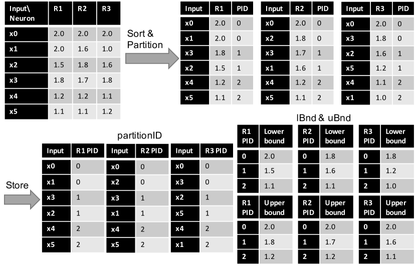
Figure 1. An example of building the Neural Partition Index of three neurons, $R1,R2,R3$, for six inputs, $x0,\dots,x5$.

There are two approaches to implementing the index. The first approach would be to maintain a set of buckets, each identified with a unique (neuronID, PID) combination as the key, and, for each bucket, maintain a list of inputIDs. The second approach, which DeepEverest uses, is to maintain a list of (neuronID, inputID) pairs as keys, and, for each entry, store the PID. neuronID, inputID, and PID are integers, so rather than building a B-tree or a hash index over the keys, we create an optimized index structure using an array where neuronID and inputID act as offsets for lookups in the array. This enables DeepEverest to only store the values and therefore avoid the cost of storing the keys. Figure 1 illustrates NPI for an example dataset with three partitions.

During preprocessing, DeepEverest runs DNN inference on all inputs once to build NPI for every neuron, which requires sorting. The time complexity to compute NPI once the activations are computed is $O(nNeurons\cdot nInputs\cdot log_{2}(nInputs))$, but the main source of overhead is DNN inference, which is a cost proportional to the number of inputs. The method that DeepEverest adopts is more space-efficient than building an index over (neuronID, PID) pairs because it costs $nNeurons\cdot nInputs\cdot\log_{2}(nPartitions)$ bits rather than $nNeurons\cdot nInputs\cdot\log_{2}(nInputs)$ bits, where $nPartitions<<nInputs$. NPI also has much smaller storage overhead compared to fully materializing all activation values. A PID takes less storage than an activation value because a PID only costs $log_{2}(nPartitions)$ bits, while an activation value is usually a 32-bit floating point. For example, if DeepEverest has $8$ partitions for each neuron, representing a PID costs 3 bits, which is less than $10\%$ of the storage cost of full materialization. Storing the lower and upper bounds costs $nNeurons\cdot nPartitions\cdot 2\cdot 32$ bits, which is normally negligible compared to the cost of storing the PIDs.

4.4. Neural Threshold Algorithm (NTA)

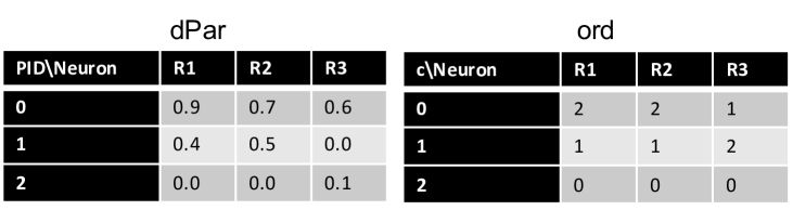
Figure 2. $dPar$ and $ord$ for the execution of NTA for the example query that finds the most similar inputs to $x5$ based on the activations of $\{R1,R2,R3\}$. For neuron $i$, $c$ is the index of the PIDs in $ord(i)$, e.g., when $c{=}0$, $ord(R1,c){=}2$.

(a) Build $toRun$

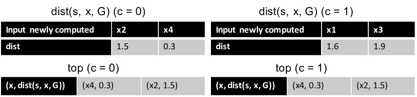
(b) Perform DNN inference to compute $dist$ and update $top$

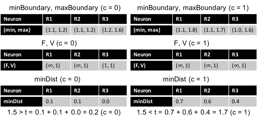
(c) Check termination

Figure 3. Intermediate variables for the execution of NTA for the example query. The values when $c{=}0$ are shown on the left, and the values when $c{=}1$ are shown on the right.

Notation. We denote with $N$ the set of all neurons in the DNN and with $D$ the input dataset. A neuron is denoted with $n{\in}N$ and an input with $x{\in}D$. $x$ is the inputID. The user issues a query: topk($s,G,k,\textsc{dist}$), where $s{\in}D$ is the sample input (also known as the target input) of interest to the user. $G{\subseteq}N$ is a set of neurons from a single layer in $N$. $k$ is the desired number of query results, and dist is the distance function. This function computes the distance between the set of activations of $s$ and $x$ looking only at the neurons in $G$. Table 2 lists our frequently used notation.

Table 2. Summary of frequently used notation.

Symbol	Meaning
$s$	Sample input (or target input) from $D$
$G$	Group of neurons from $N$
topk($s,G,k,$dist)	Top-$k$ most-similar query
dist	Function to compute distances between inputs
$g_{i}$ (or $i$ when clear)	The $i$-th neuron in $G$
$\texttt{act}(i,x)$	Activation value of $g_{i}$ for input $x$
$dist(s,x,G)$	Distance between $s$ and $x$ based on $G$
$top$	Set of top-$k$ inputs that are closest to $s$
$P_{n}$	Set of partitions for neuron $n$
getInputIDs$(n,p)$	inputIDs of a single partition $p{\in}P_{n}$
sPID$(n)$	PID to which $s$ belongs for neuron $n$
lBnd$(n,p)$	Lower bound of a single partition $p{\in}P_{n}$
uBnd$(n,p)$	Upper bound of a single partition $p{\in}P_{n}$

NTA returns the set of top-$k$ inputs that are closest to the target input when considering only the neurons in $G$. This set of top-$k$ inputs can be defined as a set $top\subseteq D$ of $k$ inputs. $top$ is initially empty and is conceptually built incrementally by identifying and adding to $top$ the next input that satisfies:

(1) $$\arg\min_{x{\in}D\setminus top}\left\{dist(s,x,G)\right\}$$

We further denote with $g_{i}$ (or $i$ when clear) the $i$-th neuron in set $G$, and with act$(i,x)$ the activation of neuron $g_{i}$ on input $x$. $g_{i}$ is the neuronID. For each neuron $n{\in}N$, NPI includes the set of partitions, $P_{n}$. We denote a single partition for neuron $n$ with $p{\in}P_{n}$, and $p$ is the PID. We denote the lower and upper bounds of this partition $p{\in}P_{n}$ with lBnd$(n,p)$ and uBnd$(n,p)$.

NTA proceeds as follows,

Step 1: Load indexes. We assume that NPI is initially on disk. This step reads the NPI for the neurons $g_{i}{\in}G$ from disk. The index holds the set of partitions, their lower and upper bounds, and the PIDs of each input for each $g_{i}{\in}G$.

Step 2: Compute target activations. For each $g_{i}{\in}G$, compute act$(i,s)$, the activation value for input $s$ and neuron $g_{i}$ by running DNN inference on input $s$. A single inference pass is sufficient to compute the activations for all neurons in $G$.

Step 3: Order partitions. This step computes the order by which the partitions are accessed by NTA for each neuron. Let $\texttt{sPID}(i)$ denote the PID to which $s$ belongs for neuron $g_{i}$. For each neuron $g_{i}{\in}G$ and partition $p{\in}P_{i}$, compute $dPar(i,p)$ as,

(2) $$dPar(i,p)=\begin{cases}0,&p=\texttt{sPID}(i)\\ \texttt{lBnd}(i,p)-\texttt{act}(i,s),&p<\texttt{sPID}(i)\\ \texttt{act}(i,s)-\texttt{uBnd}(i,p),&p>\texttt{sPID}(i)\end{cases}$$

which is the distance between the target input’s activation value for neuron $g_{i}$ and the closest activation value in partition $p$. For each neuron $g_{i}$, sort the partitions in $P_{i}$ on their $dPar(i,p)$ values in ascending order and put them in a list, denoted with $ord(i)$. Later steps will process the partitions in the order specified by $ord(i)$.

Example: To illustrate the first three steps, consider a query topk($x5,\{R1,R2,R3\},2,l1$-distance) that finds the top-$2$ most similar inputs to $x5$ based on the activations of $\{R1,R2,R3\}$, using the example dataset in Figure 1. In this example, $s{=}x5$, $G{=}\{R1,R2,R3\}$. Step 1 reads from disk PID, lBnd, and uBnd shown in Figure 1. Step 2 runs DNN inference to compute the activations for $x5$, $(\texttt{act}(R1,x5),\texttt{act}(R2,x5),\texttt{act}(R3,x5)){=}(1.1,1.1,1.2)$. Step 3 computes $dPar$ and $ord$ for $\left\{R1,R2,R3\right\}$, as shown in Figure 2.

Step 4: Find top-k. This step runs the modified threshold algorithm. It starts with the partitions to which the target input belongs, and it expands its search from there. Unlike CTA, this step incrementally computes the activations for candidate inputs and does so in batches to get good GPU performance. This step proceeds as follows,

Starting with an index $c=0$:

Step 4 (a): For each neuron $g_{i}$, maintain a set $toRun_{i}$ that contains the inputs whose activations should be computed. Access $ord(i,c)$ to get the partition that contains the next most similar inputs. Query NPI to get the inputIDs that belong to this partition $ord(i,c)$ and add them to $toRun_{i}$, i.e., $toRun_{i}{\leftarrow}\texttt{getInputIDs}(i,ord(i,c))$.

Example: as shown in Figure 3a, when $c=0$, $toRun_{R1,0}=\left\{x4,x5\right\}$ because $ord(R1,0)=2$.

Step 4 (b): For each neuron $g_{i}$, compute the activations for the inputs in $toRun_{i}$ (excluding those that have already been computed) by running DNN inference in batches. $toRun_{i}$ is cleared after DNN inference. Note that this inference step computes the activations for all neurons in the neuron group being queried. Compute the distance between each newly computed input $x$ and the target input $s$ as $dist(s,x,G)=\textsc{dist}(|\texttt{act}(0,x)-\texttt{act}(0,s)|,\dots,|\texttt{act}(|G|-1,x)-\texttt{act}(|G|-1,s)|)$. Update $top$ if $dist(s,x,G)$ is one of the $k$-smallest NTA has seen so far, i.e., input $x$ is one of the $k$-most similar inputs to the target input $s$ seen so far. Ties are broken arbitrarily.

Example: as shown in Figure 3b, when $c{=}0$, the activations of inputs $x2,x4$ are computed ($x5$ was computed in Step 1). The distances from $x2$ and $x4$ to $x5$ are $1.5$ and $0.3$, respectively.

Step 4 (c): Maintain a range of seen activations for inputs from $toRun_{i}$ for each neuron $g_{i}$, which is the range of activations such that NTA has seen every input with an activation in the open interval of this range. It is possible that NTA has seen one or more inputs from other neurons’ $toRun$ sets with activations outside of this range. However, the open interval of this range denoted by $(minBoundary_{i},maxBoundary_{i})$ only contains the activations for the inputs that NTA is guaranteed to have seen.

Let $minDist_{i}$ be the shorter distance from the boundaries of this range to the target input for each neuron $g_{i}$: $minDist_{i}=\min\left\{F_{i}{\cdot}|minBoundary_{i}{-}\texttt{act}(i,s)|,V_{i}{\cdot}|maxBoundary_{i}{-}\texttt{act}(i,s)|\right\}$, where $F_{i}$ is an indicator function that indicates whether NTA has seen the last partition (inputs with lowest activations) of neuron $g_{i}$, and $V_{i}$ is another indicator function that indicates whether the $0$-th partition (inputs with highest activations) of neuron $g_{i}$ has been seen. Specifically, $F_{i}{=}\infty$ when the last partition of neuron $g_{i}$ has been seen; $F_{i}{=}1$ otherwise. $V_{i}{=}\infty$ when the first partition of neuron $g_{i}$ has been seen; $V_{i}{=}1$ otherwise. Define the threshold to be,

(3) $$t=\textsc{dist}(minDist_{0},minDist_{1},\dots,minDist_{|G|-1})$$

The threshold, $t$, represents the smallest possible distance to $s$ from any unseen input. Hence, the termination condition is,

(4) $$\max_{x\in top}\left\{dist(s,x,G)\right\}\leq t$$

where $\max_{x\in top}\left\{dist(s,x,G)\right\}$ represents the maximum distance to the target input $s$ in the current top-$k$ result set. As soon as this inequality holds, halt and return $top$ as the query results.

Example: as shown in Figure 3c, $minBoundary_{i}$, $maxBoundary_{i}$ and $minDist_{i}$ are maintained and calculated for $\left\{R1,R2,R3\right\}$. For example, when $c=0$, $minBoundary_{R1}=1.1$, $maxBoundary_{R1}=1.2$. Since NTA has seen the last partition (2) and has not seen the first partition (0), $F_{R1}=\infty,V_{R1}=1$. Therefore, $minDist_{R1}=|maxBoundary_{R1}-act_{R1,x5}|=|1.2{-}1.1|=0.1$.

When $c=0$, ${t=0.2<1.5=\max_{x\in top}\left\{dist(s,x,G)\right\}}$, so NTA does not halt. When $c=1$, $t=1.7\geq 1.5=\max_{x\in top}\left\{dist(s,x,G)\right\}$, so NTA halts and returns $top$ as the query result. It is worth noting that the cost of DNN inference on $x0$ is not incurred because it is impossible for $x0$ to be one of the top-$2$ results.

Step 4 (d): Increment $c$ by $1$. Repeat Step 4 (a) - (d) until all partitions have been seen or the halting condition in Step 4 (c) is satisfied.

function answerQuery($model,D,s,G,k,\textsc{dist}$) $\triangleright$ $model$: the DNN, $D$: dataset, $s$: sample image, $G$: neuron group, $k$: number of results to return, dist: function to compute distances between inputs

     $layer\leftarrow\textsc{getLayer}(G)$

     $P,\texttt{lBnd},\texttt{uBnd}\leftarrow\textsc{loadIndex}(layer)$ $\triangleright$ Load indexes

     for all $g_{i}\in G$ do $\triangleright$ $P_{i}$ contains the partitions for neuron $g_{i}$

         $P_{i}\leftarrow\textsc{getPartitions}(P,g_{i})$      

     $sampleAct\leftarrow\textsc{modelInference}(model,layer,s)$ $\triangleright$ Compute the activations for $s$ by DNN inference

     Initialize act to an empty map that contains the activations of the neuron group for accessed inputs

     for all $g_{i}\in G$ do

         $\texttt{act}(i,s)\leftarrow sampleAct(i)$      

     for all $g_{i}\in G$ do

         $\texttt{sPID}(i)=P\mathrel{\mathchoice{\ooalign{$\displaystyle-\mkern-5.0mu-$\cr$\displaystyle>$}{}}{\ooalign{$\textstyle-\mkern-5.0mu-$\cr$\textstyle>$}{}}{\ooalign{$\scriptstyle-\mkern-5.0mu-$\cr$\scriptstyle>$}{}}{\ooalign{$\scriptscriptstyle-\mkern-5.0mu-$\cr$\scriptscriptstyle>$}{}}}\texttt{getPID}(g_{i},s)$

         Initialize the list $dPar(i)$

         for all $p\in P_{i}$ do $\triangleright$ $dPar(i,p)$: the distance from each partition $p$ for neuron $g_{i}$ to $s$

              if $p==\texttt{sPID}(i)$ then $dPar(i,p)\leftarrow 0$

              else if $p<\texttt{sPID}(i)$ then $dPar(i,p)\leftarrow\texttt{lBnd}(i,p)-\texttt{act}(i,s)$

              else $dPar(i,p)\leftarrow\texttt{act}(i,s)-\texttt{uBnd}(i,p)$                             

     for all $g_{i}\in G$ do $\triangleright$ $ord(i)$: the order by which the partitions for neuron $g_{i}$ are accessed

         $ord(i)\leftarrow\textsc{argsort}(dPar(i))$      

     for all $g_{i}\in G$ do $\triangleright$ Initialization of some variables

         $F_{i}\leftarrow 1$, $V_{i}\leftarrow 1$

         $minBoundary_{i}\leftarrow\infty$, $maxBoundary_{i}\leftarrow-\infty$      

     $c\leftarrow 0$, $top\leftarrow\emptyset$ $\triangleright$ Starting with $c=0$; $top$: current top-$k$ result set

     $inputRun\leftarrow\{s\}$ $\triangleright$ $inputRun$: set of inputs that have been run for DNN inference

     while True do

         for all $g_{i}\in G$ do

              if $ord(i,c)$ does not exist then $\textbf{return}{}\text{ }top$ $\triangleright$ Return if all partitions have been seen               

              $toRun_{i}\leftarrow P\mathrel{\mathchoice{\ooalign{$\displaystyle-\mkern-5.0mu-$\cr$\displaystyle>$}{}}{\ooalign{$\textstyle-\mkern-5.0mu-$\cr$\textstyle>$}{}}{\ooalign{$\scriptstyle-\mkern-5.0mu-$\cr$\scriptstyle>$}{}}{\ooalign{$\scriptscriptstyle-\mkern-5.0mu-$\cr$\scriptscriptstyle>$}{}}}\texttt{getInputIDs}(i,ord(i,c))$          

         if $exitFlag$ then break          

         $toRunUnion\leftarrow\bigcup_{g_{i}\in G}toRun_{i}\setminus inputRun$

         $toRunAct\leftarrow\textsc{modelInference}(model,layer,toRunUnion)$ $\triangleright$ Run DNN inference in batches

         for all $x\in toRunUnion$ do

              Initialize the list $diff$

              for all $g_{i}\in G$ do

                  $\texttt{act}(i,x)\leftarrow toRunAct_{i,x}$

                  $diff_{i}\leftarrow|\texttt{act}(i,x)-\texttt{act}(i,s)|$               

              $dist(s,x,G)\leftarrow\textsc{dist}(diff)$ $\triangleright$ Compute the distance between $x$ and $s$

              if $|top|<k$ or $dist(s,x,G)<\textsc{getMaxDist}(top)$ then

                  $\textsc{update}(top,x,dist(s,x,G))$ $\triangleright$ Update $top$ if $x$ is one of the $k$-most similar seen                        

         for all $g_{i}\in G$ do

              for all $x\in toRun_{i}$ do

                  $minBoundary_{i}\leftarrow\textsc{min}(minBoundary_{i},\texttt{act}(i,x))$

                  $maxBoundary_{i}\leftarrow\textsc{max}(maxBoundary_{i},\texttt{act}(i,x))$               

              if $ord(i,c+1)$ does not exist then $F_{i}\leftarrow\infty$               

              if $ord(i,c)==0$ then $V_{i}\leftarrow\infty$               

              $minDist_{i}\leftarrow\textsc{min}(F_{i}\cdot|minBoundary_{i}-\texttt{act}(i,s)|,V_{i}\cdot|maxBoundary_{i}-\texttt{act}(i,s)|)$          

         $t\leftarrow\textsc{dist}(minDist)$ $\triangleright$ Calculate the threshold $t$

         if $|top|==k$ and $\textsc{getMaxDist}(top)\leq t$ then break $\triangleright$ Termination condition          

         $inputRun\leftarrow inputRun\cup toRunUnion$

         $c\leftarrow c+1$      

     $\textbf{return}{}\text{ }top$

Algorithm 1 The Neural Threshold Algorithm for top-k most-similar queries.

The pseudocode is shown in Algorithm 1.

The key innovation of NTA compared to CTA is in its processing of the inputs partition-by-partition using NPI until the termination condition is met. NTA runs DNN inference on only the necessary partitions of inputs for it to be certain that it has the precise top-$k$ results when it terminates. This approach significantly reduces the number of inputs on which DNN inference is performed at query time compared to computing the activation values for all inputs at query time. It further improves query performance by utilizing batch processing on GPUs (NVIDIA, [n.d.]). Inputs that share a partition are sent to the DNN for inference all at once. NTA along with NPI also has much smaller storage overhead compared to fully materializing the activations for all inputs.

4.5. Instance Optimality of NTA

In this section, we investigate the instance optimality of NTA, which corresponds to the optimality in every instance, rather than just the worst or average case. Fagin’s paper (Fagin et al., 2003) shows that CTA is instance optimal for finding the top-$k$ items over all algorithms (excluding those that make very lucky guesses) and over all legal databases. We build on that proof to show the same for NTA.

Following the definitions in (Fagin et al., 2003), let $\mathbb{A}$ be a set of algorithms that answer our target queries, and $\mathbb{D}$ be a set of combinations of datasets and DNN models that are legal inputs. Let $cost(\mathcal{A},\mathcal{D})$ be the number of inputs in the dataset of $\mathcal{D}$ accessed by $\mathcal{A}\in\mathbb{A}$ when running $\mathcal{A}$ on $\mathcal{D}\in\mathbb{D}$. An algorithm $\mathcal{B}$ is instance optimal over $\mathbb{A}$ and $\mathbb{D}$ if $\mathcal{B}\in\mathbb{A}$ and if for every $\mathcal{A}\in\mathbb{A}$ and every $\mathcal{D}\in\mathbb{D}$,

(5) $$cost(\mathcal{B},\mathcal{D})=O(cost(\mathcal{A},\mathcal{D}))$$

We show the following theorem.

Theorem 4.1.

NTA is instance optimal for finding the top-$k$ inputs over all algorithms (excluding those that make very lucky guesses) and over all legal combinations of datasets and DNN models.

The proof follows similarly to that of Theorem 6.1 in (Fagin et al., 2003). We bound the maximal number of inputs accessed by NTA with an additive constant over CTA’s maximal sequential access depth.

Proof.

For any $\mathcal{D}{\in}\mathbb{D}$, assume that we already have the relation of sorted absolute differences (denoted with AbsDiff) between the activations of all inputs and the activation of the target input. Assume that CTA halts at depth $d_{i}$ for each neuron $g_{i}$ when running on AbsDiff, i.e., $d_{i}$ is the number of inputs seen via sequential accesses for neuron $g_{i}$. As in (Fagin et al., 2003), it suffices to bound the maximal number of inputs accessed by NTA for any $g_{i}{\in}G$. Let $d=\max_{i}d_{i}$. For the duration of this proof, let $x_{j}$ denote the input at depth $j$ in AbsDiff for a neuron $g_{i}$ that reaches depth $d$ when running CTA. Let $R$ be the partition size in NPI. We will show that NTA will have accessed $x_{j}(\forall 1{\leq}j{\leq}d)$ and terminate in at most $d+2R$ accesses.

Recall that we denote a single partition for neuron $g_{i}$ with $p{\in}P_{i}$. $p$ is the partition identifier, PID, and $\texttt{sPID}(i)$ is the PID of the target input $s$ for neuron $g_{i}$. In NPI, for $g_{i}{\in}G$, we say that a partition $p{\in}P_{i}$ is an above partition if $p<\texttt{sPID}(i)$; a partition $p{\in}P_{i}$ is an under partition if $p\geq\texttt{sPID}(i)$. We say that an input is an above input if it belongs to an above partition; an input is an under input if it belongs to an under partition. As in eq. 2, an above partition uses the input whose activation is the lower bound of the partition as its representative; an under partition uses the input whose activation is the upper bound as its representative (the only exception is that the partition $p=\texttt{sPID}(i)$ uses the target input, $s$, as its representative).

Without loss of generality, assume that $x_{d}$ is an above input. Let $a$ be the greatest $j{<}d$ where $x_{j}$ is an under input. Let $b$ be the least $j{>}d$ where $x_{j}$ is an under input. When NTA has accessed $x_{j}(\forall 1{\leq}j{\leq}d)$ and confirmed that $x_{b}$ is more distant from $s$ than $x_{d}$, it knows that it has the correct top-$k$ results and can then terminate. This is equivalent to the termination condition in Section 4.4.

Case 1: When $x_{a}$ is accessed by NTA after $x_{d}$, we will show at most $R$ above inputs, $x_{j}(j{>}d)$, are accessed before $x_{a}$. Assume towards contradiction that more than $R$ above inputs $x_{j}(j{>}d)$ are accessed before $x_{a}$. There would be a representative of an above partition, $x_{d^{\prime}}$ where $d^{\prime}\geq d$. Let $x_{a^{\prime}}$ be the representative of the partition containing $x_{a}$. Thus, $a^{\prime}\leq a<d\leq d^{\prime}\implies a^{\prime}<d^{\prime}$. This is a contradiction because the above partition with $x_{d^{\prime}}$ as its representative was chosen to be accessed earlier than the under partition with $x_{a^{\prime}}$ as its representative, which implies $d^{\prime}\leq a^{\prime}$.

Since under partitions are accessed in order w.r.t. $x_{a}$, the number of under inputs, $x_{j}(j{>}d)$, accessed by NTA is also at most $R$, i.e., the under inputs co-located on the partition containing $x_{a}$.

Note that if $x_{a}$ and $x_{b}$ belong to the same partition, NTA will terminate after this partition. If $x_{a}$ and $x_{b}$ belong to different partitions, then $x_{b}$ is the representative of its partition. After confirming that $x_{b}$ is more distant from the target input $s$ than $x_{d}$, NTA knows that it does not need to access any further partitions (including the partition containing $x_{b}$) and terminates. In either scenario, the number of above $x_{j}(j{>}d)$ accessed by NTA is at most $R$, and the number of under $x_{j}(j{>}d)$ accessed is also at most $R$. Hence, the total number of accesses made by NTA is at most $d+2R$.

Case 2: When $x_{b}$ is accessed by NTA before $x_{d}$, there can be at most $R$ under inputs, $x_{j}(j{>}d)$, that are accessed before $x_{d}$. Furthermore, the number of above inputs, $x_{j}(j{>}d)$, accessed is at most $R$, i.e., the above inputs co-located on the partition containing $x_{d}$. Hence, the total number of accesses made by NTA is at most $d+2R$. The proof follows similarly to Case 1.

Case 3: When $x_{a}$, $x_{b}$ are accessed by NTA in order w.r.t. $x_{d}$, $x_{b}$ must be the representative for its partition. After NTA processes the partition containing $x_{d}$, it will recognize that $x_{b}$ is more distant than $x_{d}$ and terminate. Thus no under $x_{j}(j{>}d)$ will be explicitly accessed. The above partitions are accessed in order w.r.t. $x_{d}$, so the number of above inputs, $x_{j}(j{>}d)$, accessed is at most $R$, i.e., the inputs co-located on the partition containing $x_{d}$. Hence, the total number of accesses made by NTA is at most $d+R$.

Since the three cases above exhaust all possibilities, this proves that for each neuron in $G$, NTA will have accessed $x_{j}(\forall 1{\leq}j{\leq}d)$ and terminate in at most $d+2R$ accesses. ∎

4.6. Incremental Indexing

As shown in Section 5, the DeepEverest approach described so far achieves excellent query execution times with low storage overhead. This approach, however, incurs a potentially high preprocessing cost, especially for large datasets and models. Before executing any query, DeepEverest needs to compute the activations for all neurons and all inputs by running DNN inference. It then needs to construct the indexes for all layers and persist them to disk.

To address this challenge, we propose building the indexes incrementally as queries execute so that preprocessing is performed only for the layers users query. With this approach, DeepEverest performs no preprocessing ahead of time. When the user submits a query, if the indexes of the queried layer are available on disk, DeepEverest proceeds as described in Sections 4.4, LABEL: and 4.7.1; otherwise, DeepEverest computes the activations of the queried layer by running DNN inference on all inputs. While doing so, it computes the query answer and returns it to the user. DeepEverest then constructs the indexes for the layer and persists them to disk. Note that DNN inference is performed starting from the first layer instead of a previously queried layer each time DeepEverest constructs the indexes for a layer because only the indexes of the queried layers are stored on disk. With this approach, the costs of index computation and persistence for each layer are incurred once the first time that layer is queried, and only if that layer is queried.

In Section 5.3, we show that DeepEverest with this incremental approach significantly outperforms other methods on multi-query workloads. While DeepEverest must do extra preprocessing to build and store its indexes compared with caching the activations directly, it accelerates significantly more queries because it is able to store the indexes for significantly more layers given a storage budget.

4.7. Optimizations

In this section, we present several important optimizations that further improve the performance of DeepEverest. The first optimization, described in Section 4.7.1, accelerates two common types of top-$k$ queries. The second optimization, described in Section 4.7.2, automatically selects DeepEverest’s configuration. The third optimization, described in Section 4.7.3, accelerates sequences of related queries, as may occur during data exploration.

4.7.1. Maximum Activation Index (MAI)

For a given target input and a layer in a DNN, the maximally activated neurons are those neurons in the layer for which the activation values for the target input are the highest. DNN interpretation often involves examining such maximally activated neurons (Srivastava et al., 2013; Zeiler and Fergus, 2014; Zhou et al., 2014; Bau et al., 2017) because they respond to the input the most and have the greatest impact on the DNN output. A common set of top-$k$ most-similar queries ask to find the top-$k$ similar inputs to a target input based on a neuron group consisting of these maximally activated neurons.

To accelerate these top-$k$ most-similar queries that target maximally activated neurons as well as top-$k$ highest queries, we introduce a straightforward yet effective optimization. The idea is for DeepEverest to store, for each neuron, a fraction of the highest activation values together with the corresponding inputIDs. We call this data structure the Maximum Activation Index (MAI), and denote this fraction of (activation, inputID) pairs for a given neuronID with MAI(neuronID). This fraction automatically becomes each neuron’s $0$-th partition. We denote the fraction of the inputs stored in MAI with $ratio$, which is a configurable parameter and discussed further in Section 4.7.2.

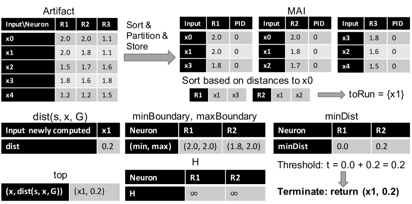
Figure 4. An example of constructing MAI ($ratio{=}0.6$) and query execution for topk($x0,\{R1,R2,R3\},1,l1$-distance) ($batchSize{=}1$). Despite $x0$ only being in MAI for $R1$ and $R2$, DeepEverest leverages MAI to answer the query after only running DNN inference on $x0$ and $x1$.

DeepEverest utilizes MAI during query execution to further reduce the number of inputs on which DNN inference is performed, if possible. DeepEverest now has more detailed knowledge of which inputs are most similar to the target input, rather than just the high-level knowledge that the inputs are in the same partition. We observe empirically that the activation values of the maximally activated neurons for an input are often likely to be in the top activations stored in MAI, and thus MAI is effective in improving the query time. DeepEverest modifies query execution described in Section 4.4 of partition $0$ to incorporate this information as follows: it first finds the neurons for which the target input is in MAI. For these neurons, DeepEverest sorts the other inputs in the $0$-th partition by their distances to the target input $s$. Rather than performing DNN inference on all inputs in MAI for each neuron, DeepEverest builds a global $toRun$ set by adding the most similar inputs from all of these neurons until the batch size is reached. Step 4(c) in Section 4.4 is modified to compute $minDist_{i}$ as $\min\left\{|minBoundary_{i}{-}act_{i,s}|,H_{i}\cdot|maxBoundary_{i}{-}act_{i,s}|\right\}$, where $H_{i}$ is an indicator function that indicates whether NTA has seen the input with the highest activation in MAI(i). $H_{i}{=}\infty$ when highest activation of neuron $g_{i}$ has been seen; $H_{i}{=}1$ otherwise. The neurons $g_{i}$ for which $s$ is not in MAI(i) contribute $0$ to the threshold calculation. Figure 4 illustrates an example.

4.7.2. Automatic Configuration Selection

Given a storage budget, DeepEverest must allocate it between NPI and MAI. It uses a heuristic algorithm to achieve this. A greater $nPartitions$ leads to smaller partitions, which is key to generally better performance (see Section 5.4) on queries that target any kind of a neuron group (see Section 5.1), while a larger $ratio$ accelerates only the two types of queries mentioned in Section 4.7.1. Hence, DeepEverest first picks a value for $nPartitions$ and then sets the value of $ratio$.

Intuitively when partitions are smaller, DNN inference is performed on fewer inputs not in the top-$k$ because DeepEverest processes inputs partition-by-partition. However, if the partitions are smaller than the optimal batch size, DeepEverest will not leverage the full GPU parallelism.

Given a storage budget, $budget$ (in bytes), and a batch size, $batchSize$, DeepEverest sets $nPartitions$ to be the maximum power of two (to utilize all bits) that satisfies $nPartitions\leq nInputs/batchSize$ and $cost(nPartitions)<budget$. $cost(nPartitions)$ is the bytes consumed by storing NPI and is calculated as $nNeurons\cdot nInputs\cdot\log_{2}(nPartitions)/8$. $batchSize$ is set to the value that achieves the highest throughput for the DNN. Given the remaining storage budget, DeepEverest sets $ratio$ to be the maximum value that satisfies $cost(ratio)\leq budget-cost(nPartitions)$, where $cost(ratio)$ is the bytes consumed by storing MAI and calculated as $ratio\cdot nInputs\cdot nNeurons\cdot 4\cdot 2$, since activation and inputID are 4 bytes each. When there is no remaining storage budget after selecting $nPartitions$, DeepEverest sets $ratio$ to $0$.

4.7.3. Inter-Query Acceleration (IQA)

Inter-Query Acceleration (IQA) is an optimization technique to accelerate sequences of related queries, as may occur during DNN interpretation. As an example, imagine that a user finds a misclassified image. The user may want to first see the maximally activated neurons in a layer for the image and then find images with similar maximally activated neurons. The user may then decide to change how many neurons they are looking at, e.g., go from the top-3 neurons to the top-4 neurons. Queries that overlap in neurons present an opportunity for further optimization as activation values can be reused for related queries.

With IQA, DeepEverest leverages an in-memory cache that contains recently used activation values to reduce the number of inputs that it must run DNN inference on at query time. Note that this in-memory cache is different from the disk caches described in Section 4.1. During query execution, DeepEverest inserts the activation values of each input processed by NTA into the cache. Instead of caching only the activation values for the neuron group being queried, it caches the activations for all neurons in the queried layer. This enables DeepEverest to utilize the cache for future related queries that target a different group of neurons in the same layer. DeepEverest adopts a most recently used (MRU) replacement policy for the in-memory cache. This is because DeepEverest processes partitions in order from most similar to the target input to least similar, and it seeks to prioritize keeping the activations from the most similar partitions in the cache. We show in Section 5.6 that given a small in-memory cache budget, DeepEverest with IQA achieves up to $8{\times}$ faster query times than DeepEverest without it.

5. Evaluation

DeepEverest is implemented in Python, using C++ to build the indexes. We evaluate it against the baselines described in Section 4.1.

(a)

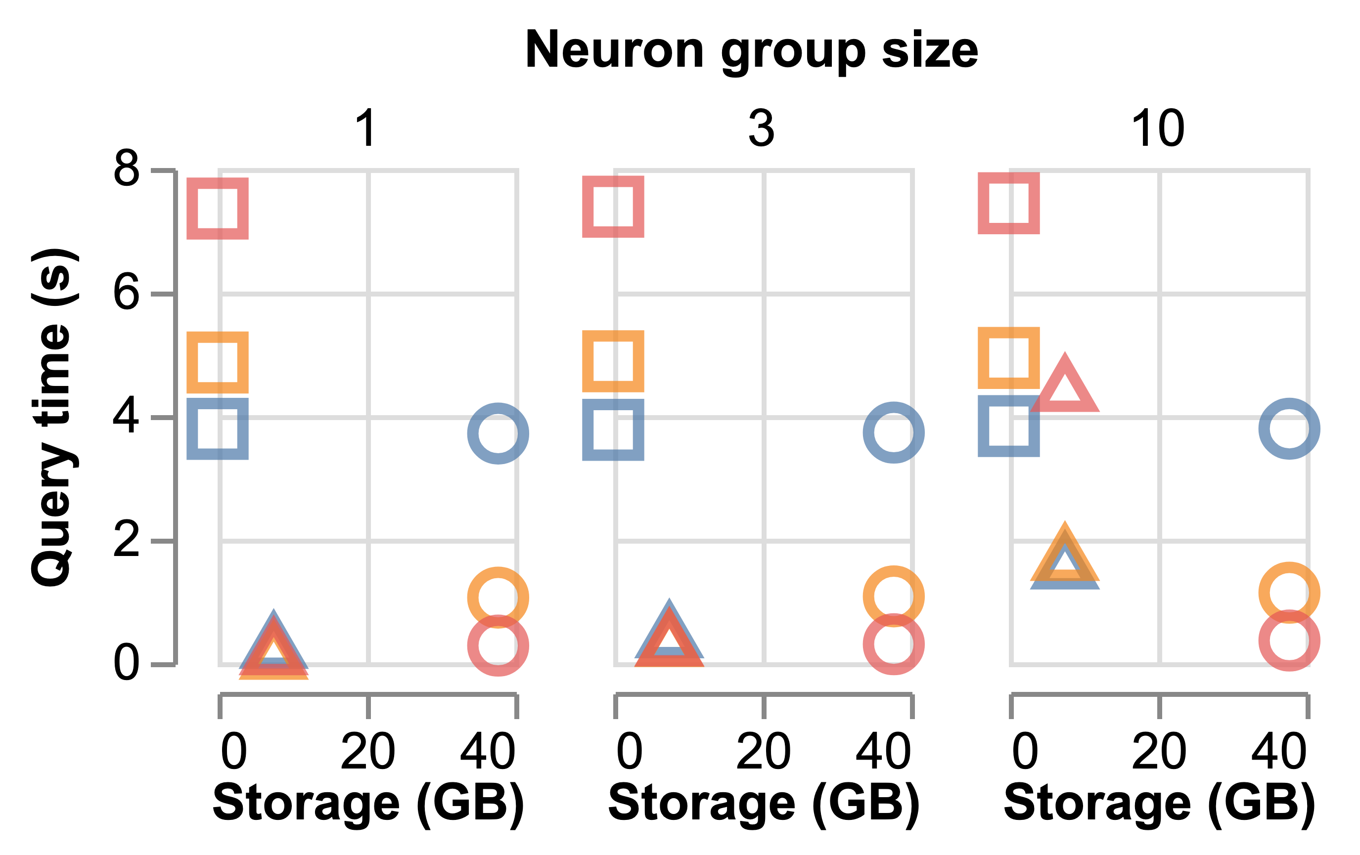
(a) FireMax, CIFAR10-VGG16

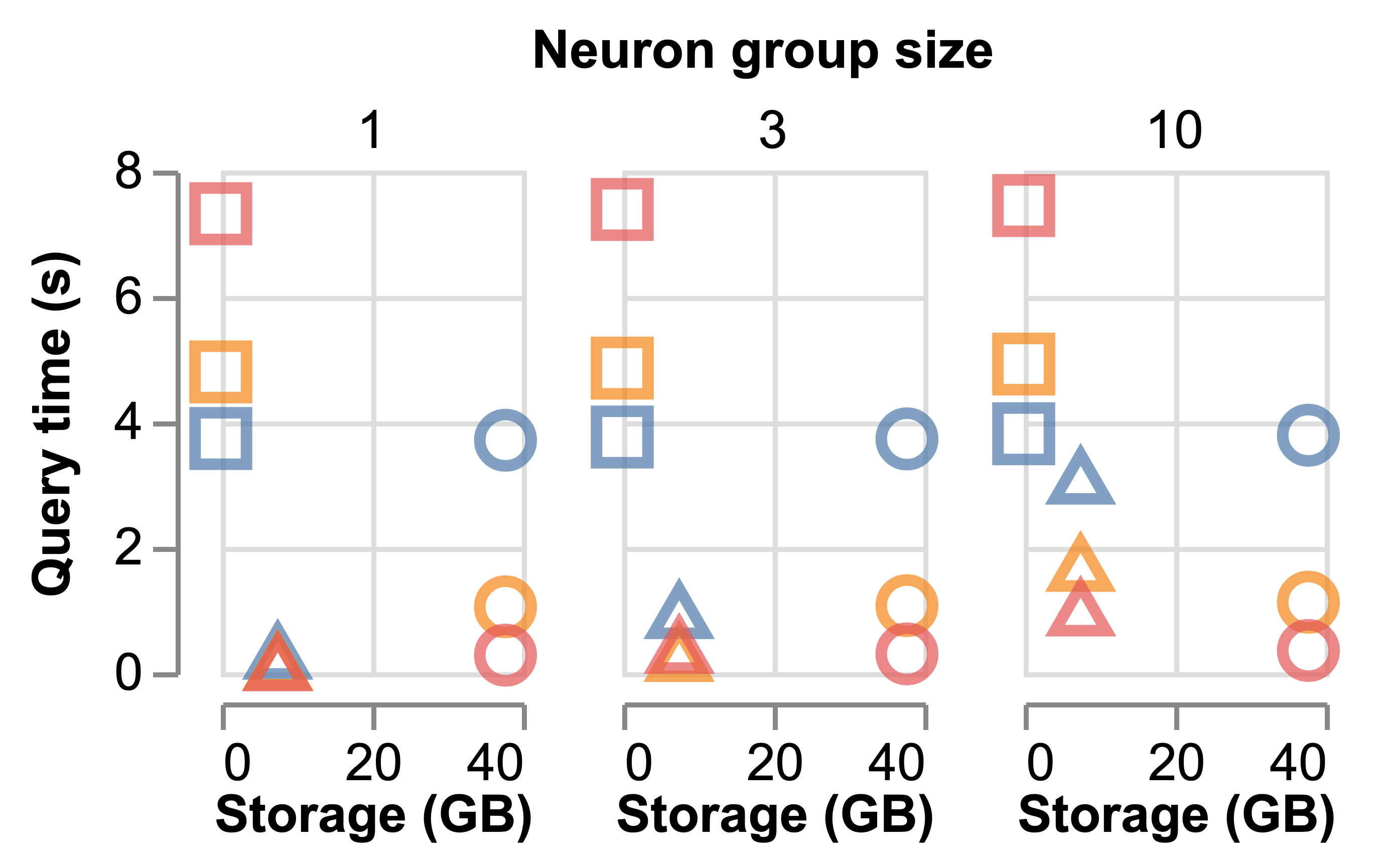
(b) SimTop, CIFAR10-VGG16

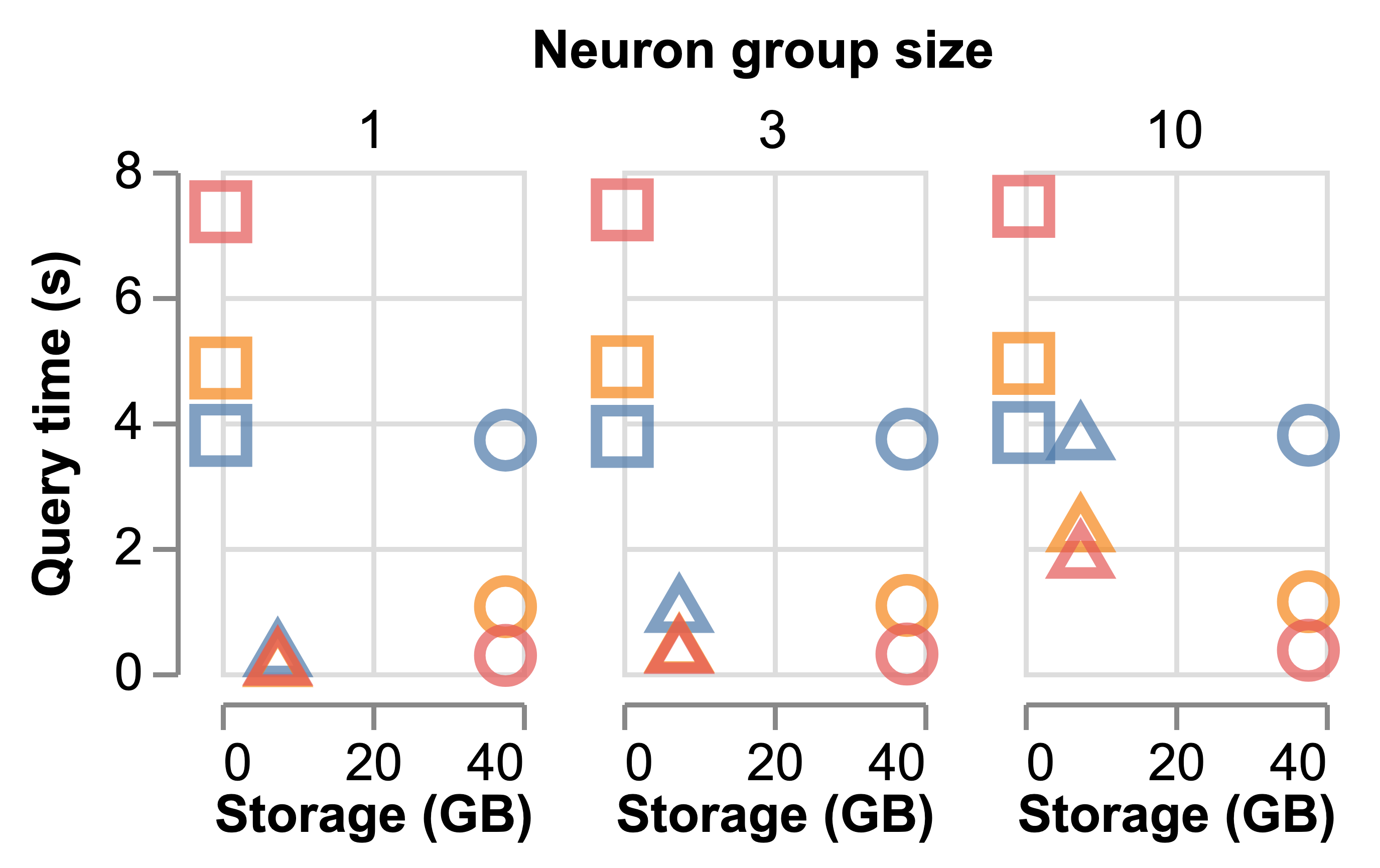
(c) SimHigh, CIFAR10-VGG16

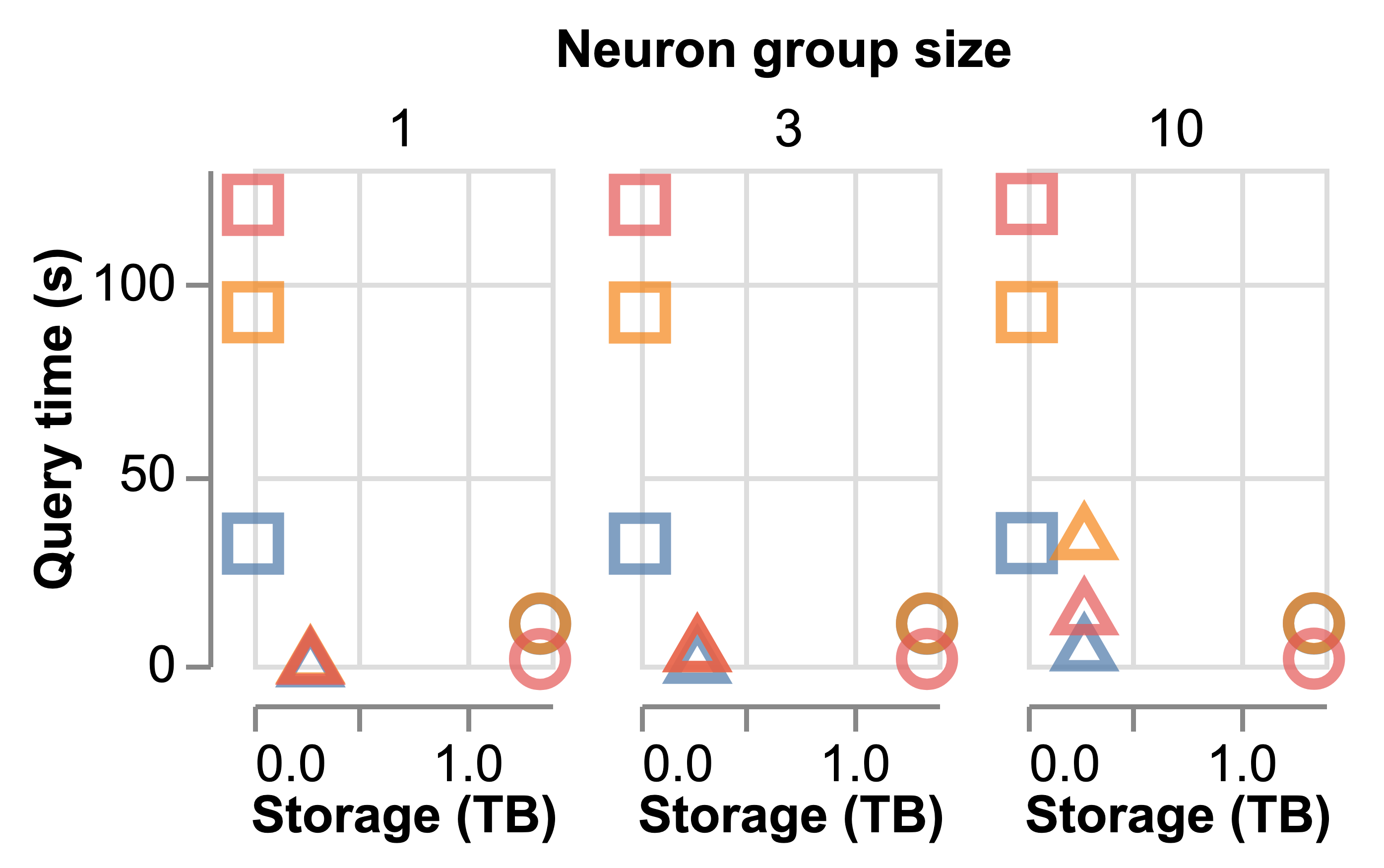
(d) FireMax, ImageNet-ResNet50

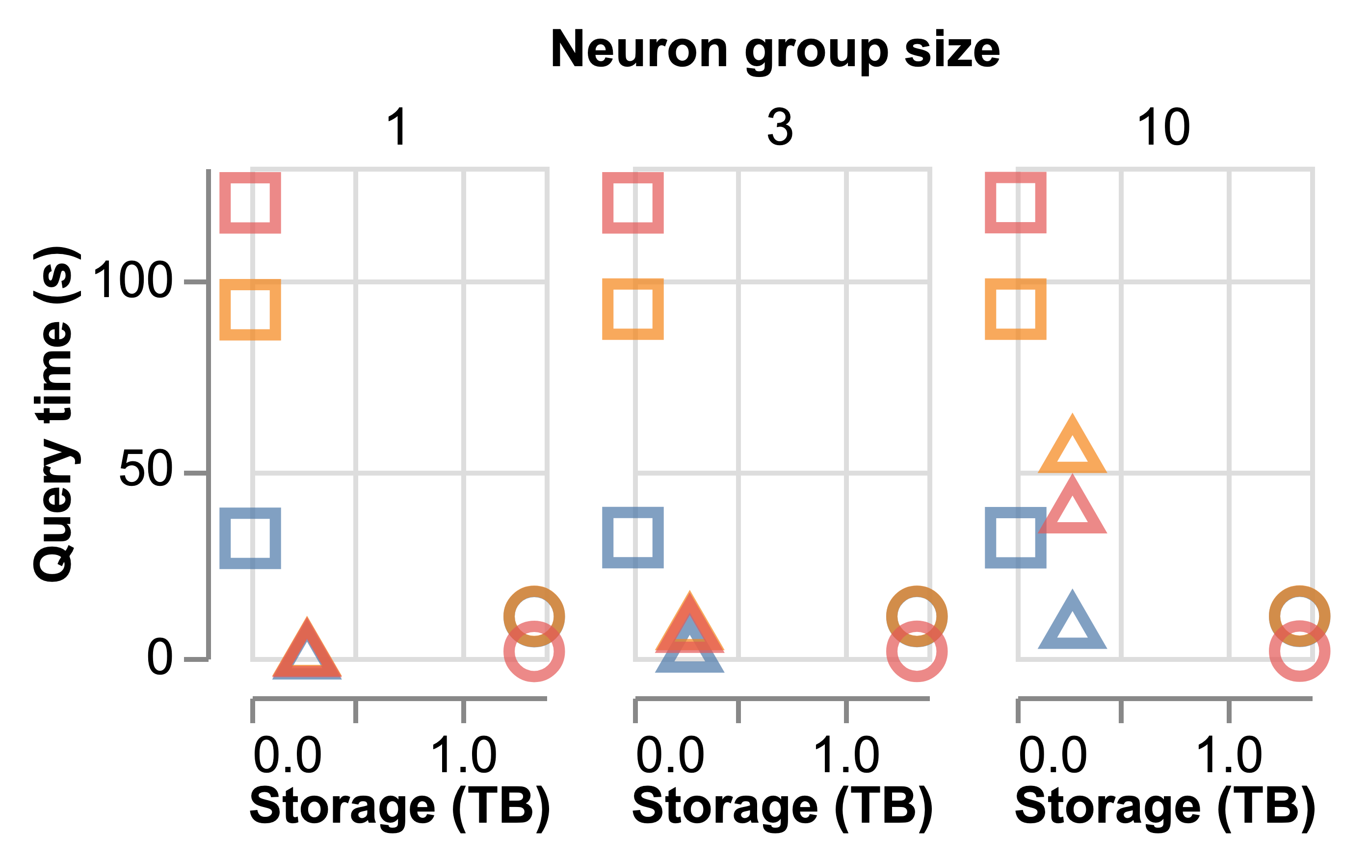
(e) SimTop, ImageNet-ResNet50

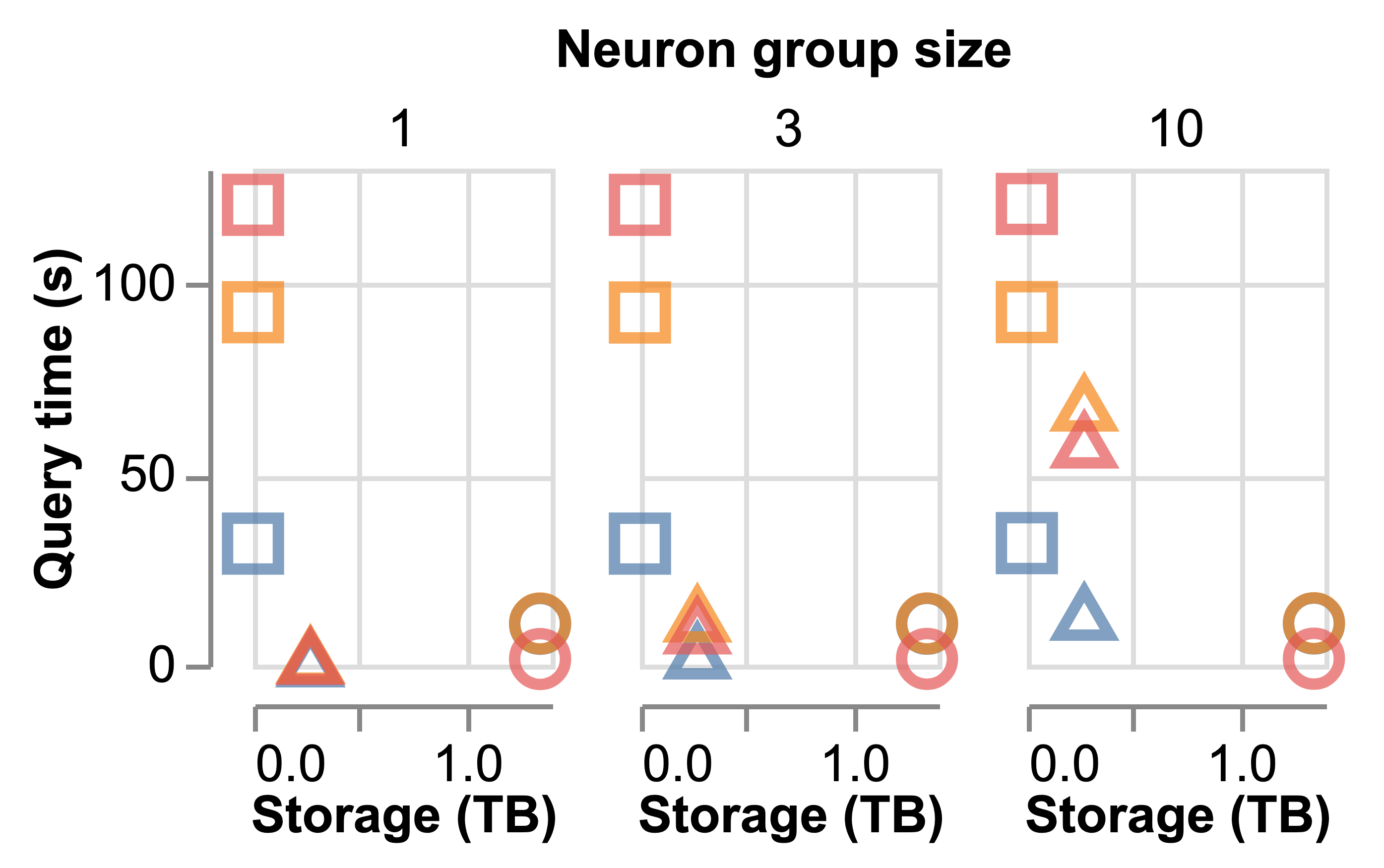
(f) SimHigh, ImageNet-ResNet50

Figure 5. End-to-end individual query times and storage sizes on CIFAR10-VGG16 and ImageNet-ResNet50. $nPartitions$ and $ratio$ of DeepEverest are selected by our heuristic algorithm given a storage budget of $20\%$ of full materialization.

5.1. Evaluation Setup

Datasets and models. We evaluate DeepEverest on two sets of well-known datasets and models. The first, called CIFAR10-VGG16, uses as inputs 10,000 images from the test set of CIFAR10 (Krizhevsky et al., 2009), and uses a VGG16 network (Simonyan and Zisserman, 2014; Liu and Deng, 2015). The second, called ImageNet-ResNet50, uses as inputs 10,000 images from the validation set of ImageNet (Russakovsky et al., 2015), and uses a ResNet50 model (He et al., 2016). These two sets of models and datasets complement each other in terms of model and input size and DNN inference cost. In all experiments, we pre-load the entire input dataset into memory. We set $batchSize$ for each model as the value that achieves the highest inference throughput (128 for CIFAR10-VGG16; 64 for ImageNet-ResNet50).

Query generation. To generate queries, we consider 3 types of layers: early, mid, and late. For CIFAR10-VGG16, these correspond to activation layers 2, 7, and 13. For ImageNet-ResNet50, we use activation layers 2, 25, and 48. Given an input and a layer, we consider the following types of neuron groups: (a) Top: the maximally activated neurons for the given input in the layer; and (b) RandHigh: neurons randomly picked from the top half of non-zero neurons for the given input. We further consider small, medium, and large neuron groups consisting of 1, 3, and 10 neurons. Finally, based on the neuron groups, we use the following query types: (a) FireMax: top-$k$ highest query; (b) SimTop: top-$k$ most-similar query based on a Top neuron group; and (c) SimHigh: top-$k$ most-similar query based on a RandHigh neuron group. We randomly select inputs from each dataset to generate SimTop and SimHigh queries.

In all experiments, we set $k{=}20$, which is a reasonable number of results for a user to inspect for a query. With a smaller $k$, we expect DeepEverest to achieve larger speedups because it will process fewer inputs and therefore return the results faster, while the query times of baselines will remain similar since they still need to recompute or load all the activations and maintain the query results. With a larger $k$, the overall speedups could degrade, but DeepEverest can incrementally return the top-$k$ query results, as discussed in Section 6. Therefore, the perceived query time is still significantly improved. We use $l_{2}$-distance as the distance function. All numbers reported are median values of five queries on random inputs for each query configuration (e.g., query type: FireMax, neuron group size: 3, layer: late).

Machine configuration. All experiments are run on an AWS EC2 p2.xlarge instance, which has an Intel Xeon E5-2686 v4 CPU running at 2.3 GHz, with 61 GB of RAM, an NVIDIA K80 GPU with 12 GB of GPU memory, and EBS gp3 volumes for disk storage.

5.2. Fundamental Space-Time Tradeoff

(a)

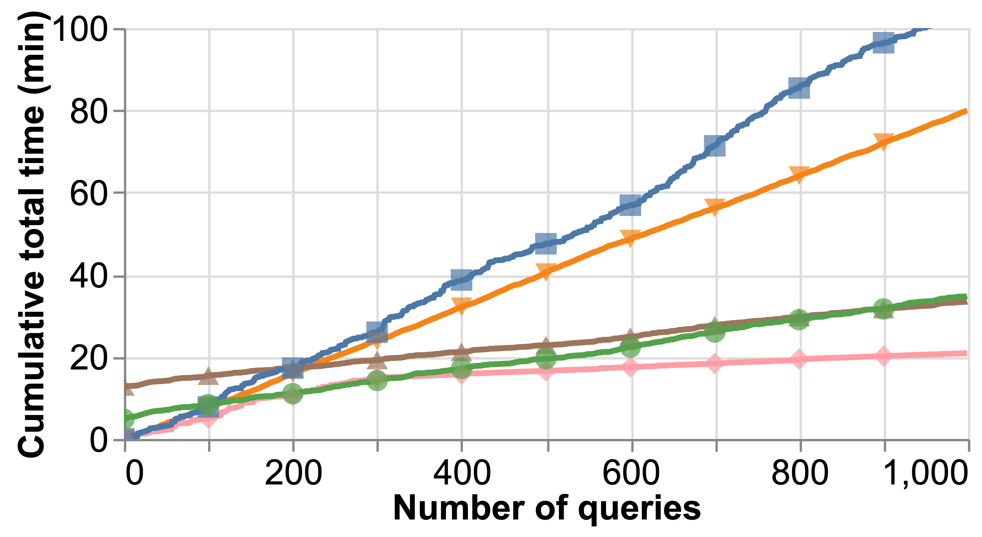
(a) Workload 1, CIFAR10-VGG16

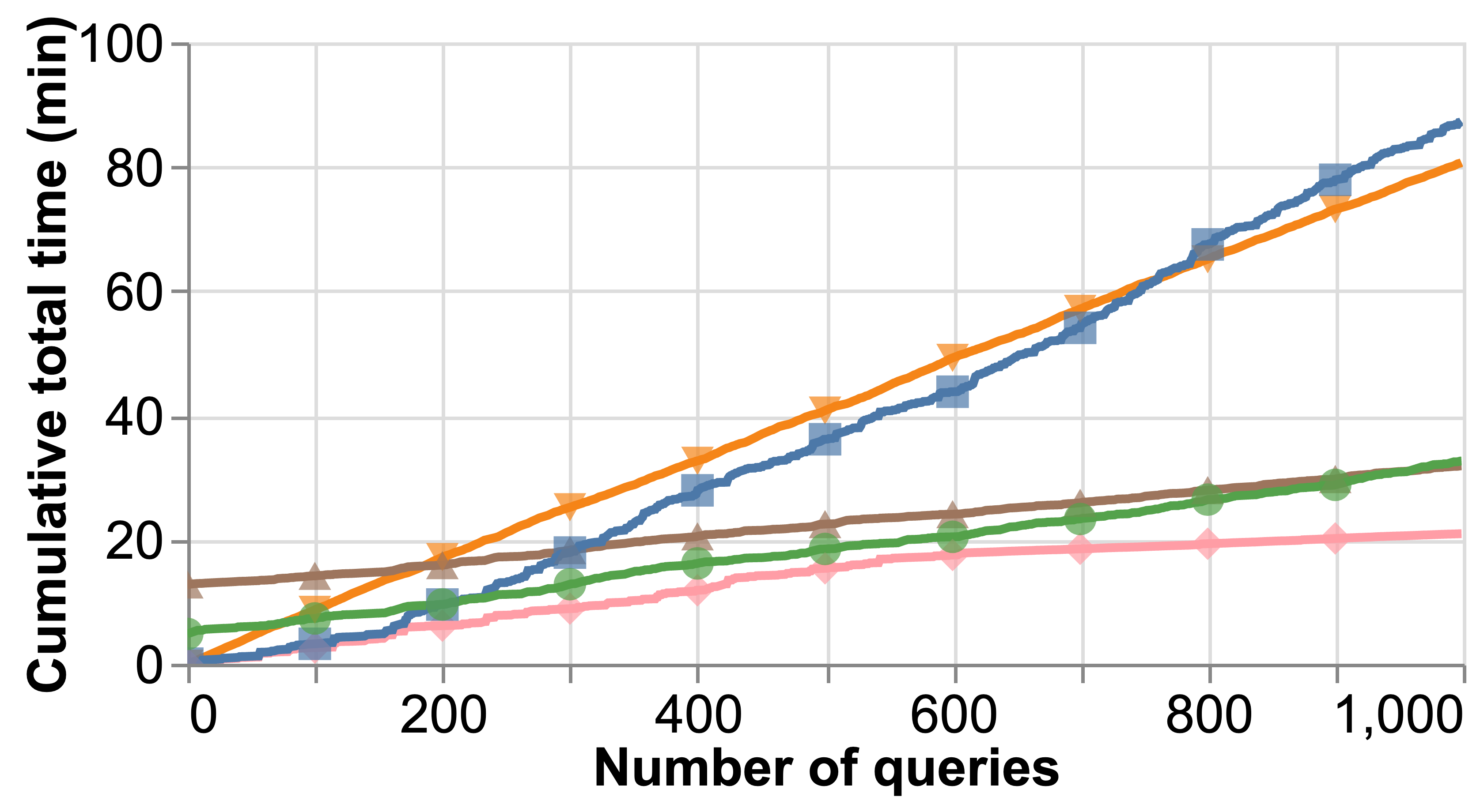
(b) Workload 2, CIFAR10-VGG16

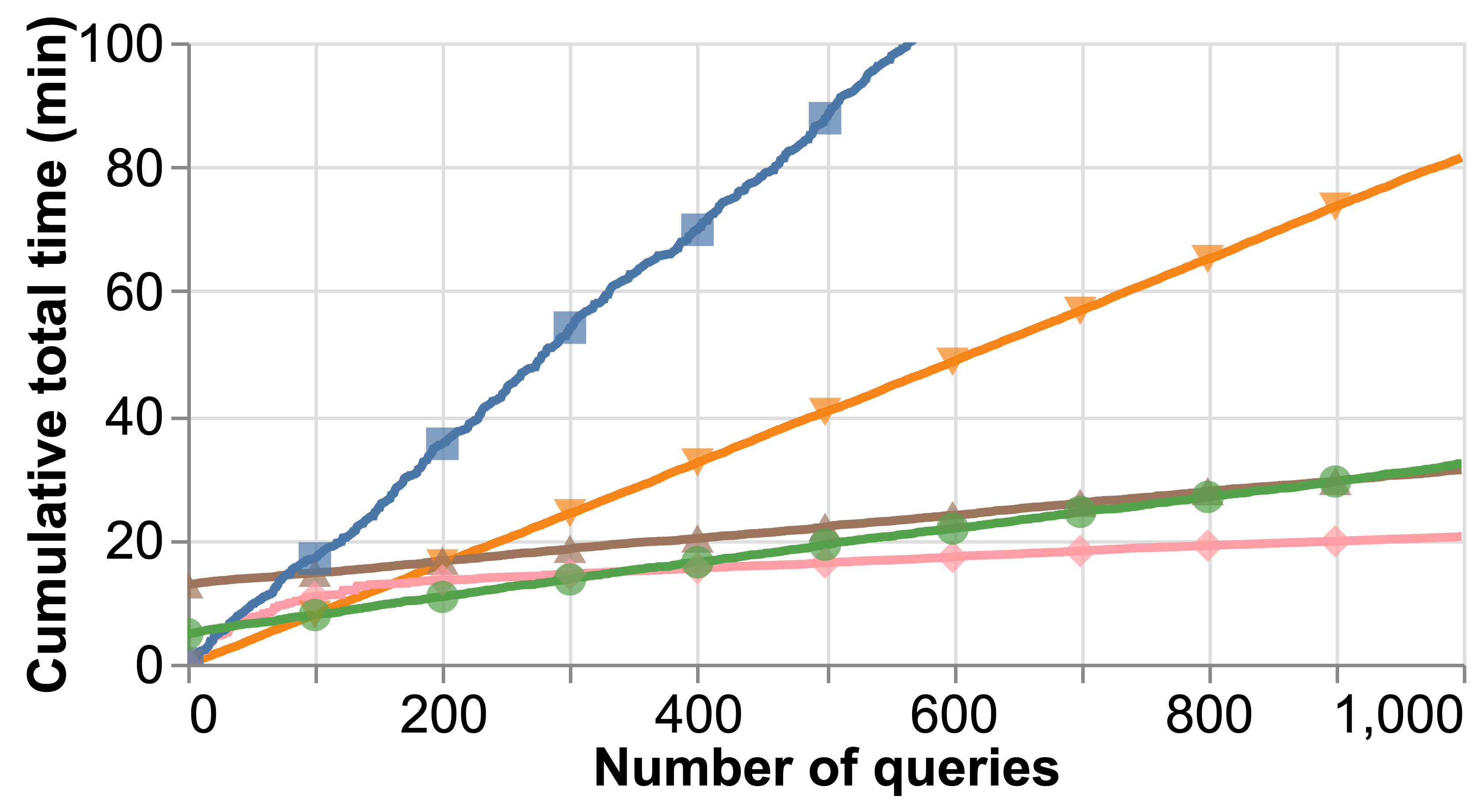
(c) Workload 3, CIFAR10-VGG16

(d) Workload 1, ImageNet-ResNet50

(e) Workload 2, ImageNet-ResNet50

(f) Workload 3, ImageNet-ResNet50

Figure 6. Cumulative total time (preprocessing time plus query execution time) for various multi-query workloads.

We first evaluate the fundamental trade-off that DeepEverest achieves in terms of storage space and query execution time for individual queries. In this experiment, the only optimization DeepEverest uses is MAI described in Section 4.7.1. We first precompute and store the indexes for all layers before executing the benchmark queries. DeepEverest has a storage budget of $20\%$ of PreprocessAll, and selects $nPartitions$ and $ratio$ using the algorithm described in Section 4.7.2. For CIFAR10-VGG16, $nPartitions=64$, $ratio=0.0046$; for ImageNet-ResNet50, $nPartitions=64$, $ratio=0.0074$. We compare DeepEverest against PreprocessAll and ReprocessAll. Figure 5 shows the results.

As the figures show, PreprocessAll has the highest storage cost (37.8 GB for CIFAR10-VGG16, and 1.35 TB for ImageNet-ResNet50) since it stores all activations for every input. However, scanning the precomputed activation values generally leads to the fastest query times. The query times of PreprocessAll are slower for the early layer of CIFAR10-VGG16 because it has a large number of neurons, and thus it takes longer to load all the activations. ReprocessAll has the lowest storage cost since it does not precompute or store anything ahead of time. Its query times are slow because of the DNN inference on the entire dataset at query time.

DeepEverest achieves the best of both worlds: low storage overhead and fast query times. For CIFAR10-VGG16, compared with ReprocessAll DeepEverest is $1.65{\times}$ to $31.1{\times}$ faster for FireMax, $1.22{\times}$ to $50.8{\times}$ faster for SimTop, and up to ${31.5\times}$ faster for SimHigh. For ImageNet-ResNet50, compared with ReprocessAll, DeepEverest is $2.67{\times}$ to $62.8{\times}$ faster for FireMax, $1.65{\times}$ to $63.5{\times}$ faster for SimTop, and $1.35{\times}$ to $63.1{\times}$ faster for SimHigh.

Compared to PreprocessAll for both CIFAR10-VGG16 and ImageNet-ResNet50, DeepEverest achieves comparable and sometimes even faster query times for queries that target small and medium-size neuron groups despite using only $20\%$ of PreprocessAll’s storage overhead. For queries that target large neuron groups, DeepEverest’s query times are slower. We observe this phenomenon again in Figure 9 (discussed in Section 5.4). Due to the curse of dimensionality, there is little difference in the distances between different pairs of inputs. As a result, DeepEverest is not able to reduce the number of inputs run by the DNN at query time as it does for small and medium neuron groups. Table 3 shows the number of inputs run by the DNN at query time to compute the activation values for SimHigh queries. We find that the number of inputs run by the DNN at query time for queries on larger neuron groups is higher than that of queries on smaller neuron groups.

5.3. Multi-Query Workloads

In this section, we evaluate DeepEverest on multi-query workloads using incremental indexing described in Section 4.6 that avoids start-up overhead. We construct various query workloads to represent possible DNN interpretation patterns and compare DeepEverest against other on-disk caching techniques. All workloads consist of $1{,}000$ the most general SimHigh queries that target neuron groups of medium size. The first query of each workload targets a RandHigh neuron group from a randomly selected layer. Each later query has probabilities $p_{same}$ of querying the same layer as the previous query, $p_{prev}$ to query one of the previously queried layers (excluding the layer queried by the previous query), and $p_{new}$ to query a layer that has not been queried yet. Workload 1 sets these to $p_{same}{=}0.5,p_{prev}{=}0.3,p_{new}{=}0.2$. Workload 2 sets these to $p_{same}{=}0.5,p_{prev}{=}0.4,p_{new}{=}0.1$. Workloads 1 and 2 are intended to simulate the exploration process of users that are likely to initially target layers they are interested in, and gradually explore more layers. Additionally, we construct Workload 3 in which queries are independent of each other; each layer is targeted uniformly at random by each query. This is not a realistic interpretation pattern but is meant to show the worst-case workload for DeepEverest.

We measure the cumulative total time, which includes the time for both preprocessing and query execution, and cumulative storage for each method. DeepEverest is given a storage budget of $20\%$ of full materialization, and $nPartitions$ and $ratio$ are selected by our heuristic algorithm. LRU Cache and Priority Cache have the same $20\%$ storage budget. The time to initially compute and store the data on disk is included with the $0$-th query for PreprocessAll and Priority Cache. The results for cumulative total time are shown in Figure 6. We report the storage results in the text.

DeepEverest consistently performs the best for Workloads 1 and 2 using less than $20\%$ of the storage of full materialization. We observe that after some number of queries, the cumulative total time of DeepEverest grows more slowly. For CIFAR10-VGG16, it plateaus after around 300 queries for Workload 1 and around 550 queries for Workload 2. This indicates that DeepEverest has built and stored NPI and MAI for all layers in the DNN. All later queries are much faster because they benefit from these indexes and NTA. For ImageNet-ResNet50, DeepEverest completes building and storing the indexes for all layers after around 780 queries for Workload 1 and never completes for Workload 2, as we observe that DeepEverest’s storage consumption is only $11.3\%$ of full materialization after 1,000 queries. DeepEverest finishes building its indexes after fewer queries in Workload 1 than in Workload 2 since Workload 1 has a higher probability of querying new layers.

While DeepEverest has the fastest query times, its storage also grows more slowly than the baseline approaches (except for ReprocessAll which does not have any storage overhead). For both datasets and models, PreprocessAll uses full storage after its preprocessing step. Similarly, Priority Cache consumes its $20\%$ storage budget after preprocessing. LRU Cache consumes its storage budget after around 50 to 200 queries. As discussed above, DeepEverest finishes building the indexes for all layers and consumes its storage budget after around 300 to 500 queries on CIFAR10-VGG16, and for ImageNet-ResNet50 it fills its storage after 780 queries for Workload 1 and never does so for Workload 2.

For Workload 3, which is unlikely an interpretation pattern, DeepEverest is slightly worse than the best performing method for the first 200 to 300 queries on both datasets and models because during that time DeepEverest builds indexes for many new layers that have not been queried before. However, DeepEverest performs the best after 400 queries because more queries target previously seen layers and benefit from its indexes and NTA.

We further observe that users typically pause between queries. DeepEverest can use that time to compute and persist its indexes to disk, which would yield even better user-perceived query times.

5.4. DeepEverest’s Configuration Selection

We now study the effectiveness of NPI and MAI, and the impact of DeepEverest’s configurable parameters, as well as how DeepEverest performs using the configuration selection heuristic described in Section 4.7.2 with different storage budgets.

(a)

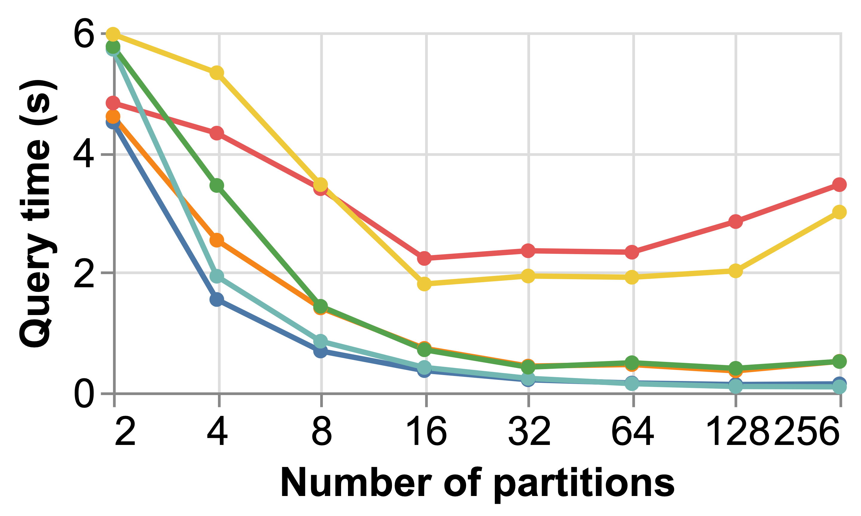
(a) CIFAR10-VGG16

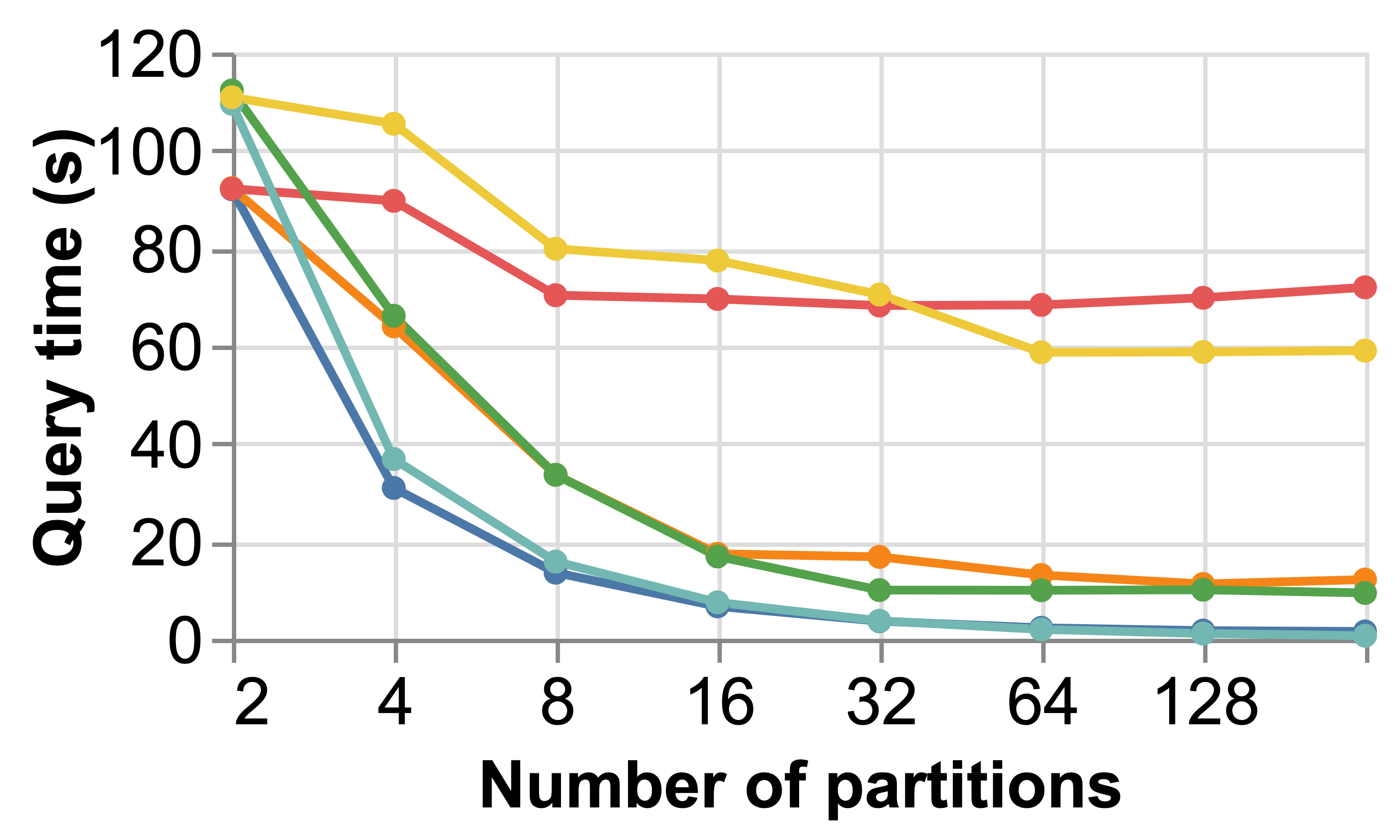
(b) ImageNet-ResNet50

Figure 7. Query times of SimHigh queries when varying $nPartitions$. Note the log scale on the $x$-axis.

(a)

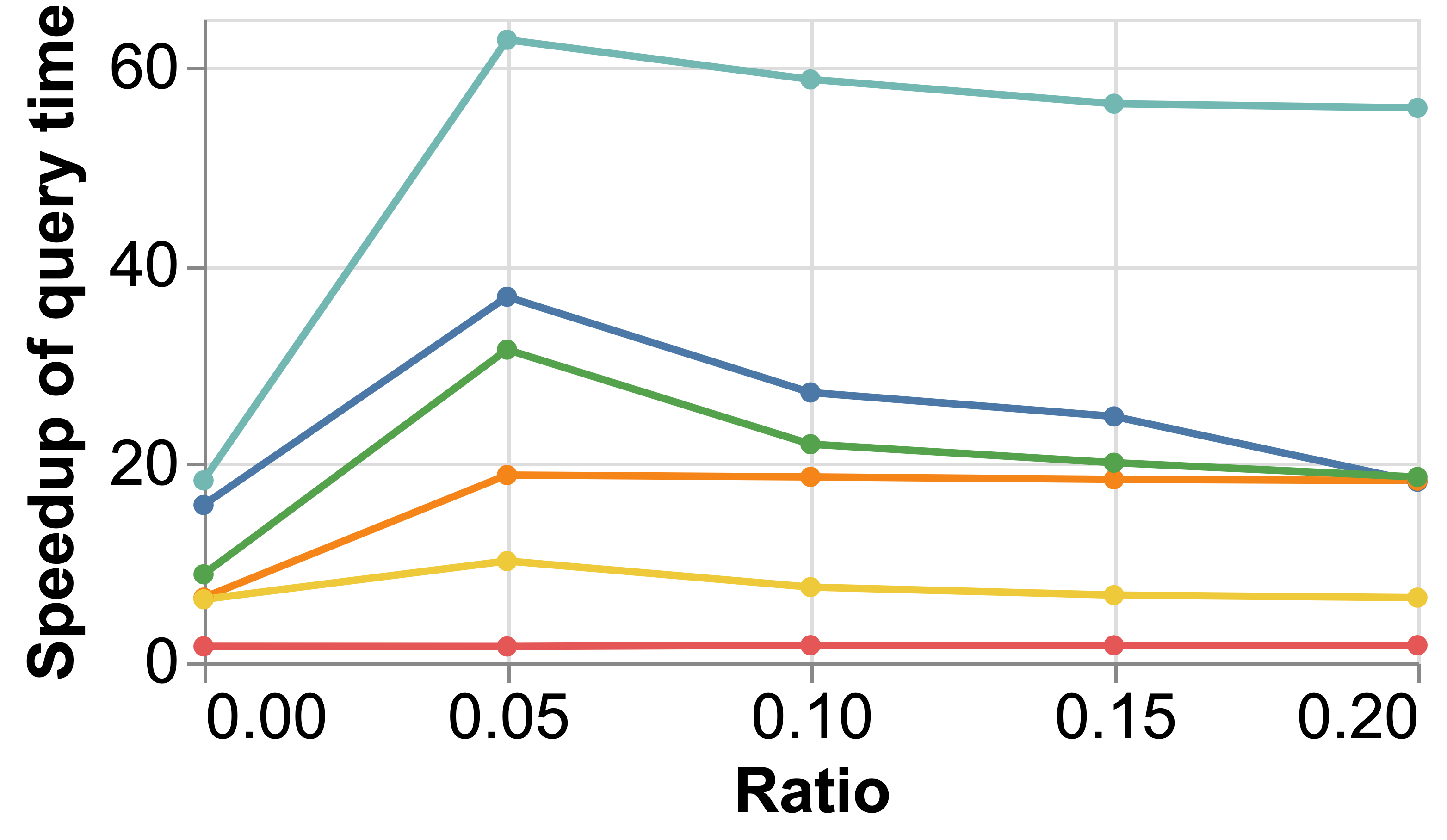
(a) CIFAR10-VGG16

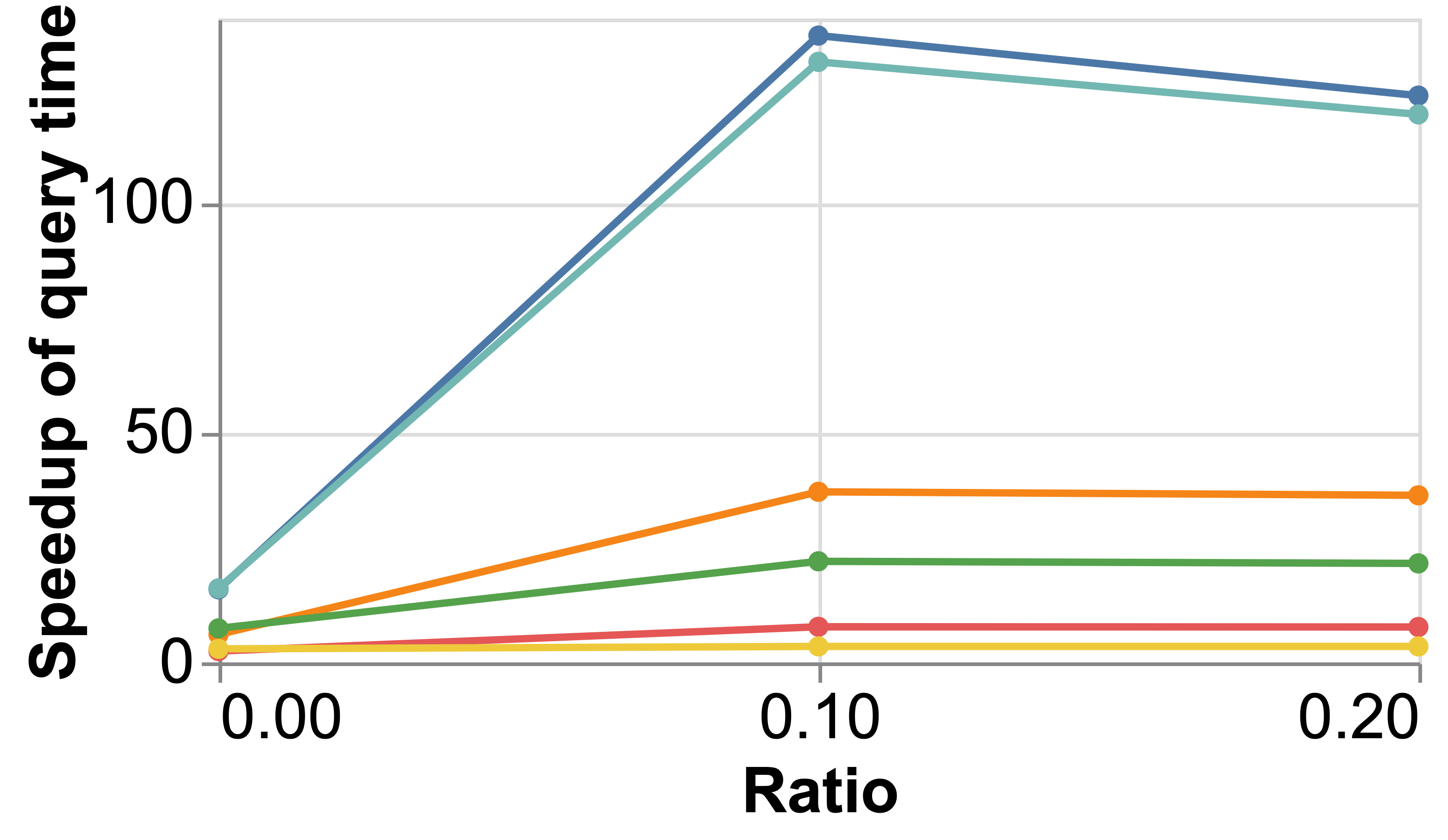
(b) ImageNet-ResNet50

Figure 8. Speedups of query times (layer: late) against ReprocessAll when varying $ratio$ with $nPartitions$ set to $16$.

Impact of Number of Partitions. We first examine how the number of partitions, $nPartitions$, affects the query times. We measure the query times of DeepEverest on SimHigh queries after building NPI with varying $nPartitions$. MAI is disabled for this experiment. The results are shown in Figure 7. We also measure the number of inputs on which DeepEverest performs DNN inference during query processing. Table 3 shows the results for CIFAR10-VGG16. Similar trends are observed for ImageNet-ResNet50.

The query time initially decreases as $nPartitions$ increases. This is because when partitions are larger, inputs that do not contribute to the result end up being processed by DeepEverest. Hence, as partitions get smaller, the number of inputs run by the DNN at query time decreases. Then, after $nPartitions$ increases past a certain value (64 for CIFAR10-VGG16; 128 for ImageNet-ResNet50), the query time no longer decreases despite the number of inputs run by the DNN at query time continuing to decrease. Recall that NTA runs inference on all inputs in a partition as it processes that partition. When $nPartitions$ is so large that the partition size is below the optimal $batchSize$ for DNN inference, the parallelism of the GPU is not fully utilized, which causes some queries to slow down. Therefore, a good value of $nPartitions$ creates partitions whose sizes are similar to the optimal $batchSize$.

Effectiveness of MAI. This experiment evaluates the effectiveness of MAI. We measure the speedups of query times compared with ReprocessAll when varying $ratio$, which determines the fraction of inputs with activation values materialized in MAI. Recall that when MAI is non-empty, it becomes the $0$-th partition. For this experiment, we set $nPartitions=16$, which is a setting that performs well (see Figure 7). As discussed in Section 4.7.1, MAI is designed to accelerate FireMax and SimTop queries. We measure the speedups of such queries on neuron groups of different sizes.

Figure 8 shows the results. Note that when $ratio{=}0$, DeepEverest runs without MAI. The speedups of query times are generally much higher when $ratio$ is any non-zero value. This is because MAI enables DeepEverest to return the query results after processing a subset of the inputs from MAI (partition $0$), rather than processing the entire partition. We also observe that the speedups of query times plateau or drop as $ratio$ further increases. This is because loading MAI from disk takes longer as $ratio$ increases. When a small index provides enough information for DeepEverest to find the top-$k$ results after processing only some inputs from MAI, increasing $ratio$ degrades the speedups; the additional inputs in MAI do not improve the query times, and loading a larger index takes longer. The best value of $ratio$ in practice depends on the queries and the distributions of the activations of the queried neuron group. Empirically, we observe that a small value of $ratio$ (e.g., 0.05) is good for FireMax and SimTop queries on the two datasets and models.

Table 3. Number of inputs run by the DNN at query time for SimHigh queries on CIFAR10-VGG16.

Layer-Neuron group size	Number of partitions
	4	8	16	32	64	128	256
mid-1	3334	1429	667	323	159	79	40
mid-3	5462	2902	1441	736	727	390	390
mid-10	8941	6869	4339	4215	3515	3492	3316
late-1	3334	1429	667	323	159	79	40
late-3	5968	2372	1106	618	618	388	391
late-10	9008	5565	2870	2745	2227	1956	1919

Impact of Storage Budget. In previous sections, we examined the performance of DeepEverest with a storage budget of $20\%$ of full materialization. Here we examine how well DeepEverest performs when the configuration selection algorithm has different storage budgets. We measure the speedups of query times compared with ReprocessAll for SimTop and SimHigh queries that target medium and large neuron groups, as shown in Figure 9. We observe that empirically DeepEverest delivers high speedups across different storage budgets, which also suggests that our configuration selection algorithm is robust. With a larger storage budget, DeepEverest performs better. We also observe that the speedups of queries on medium neuron groups are generally greater than the speedups for queries on large neuron groups due to the curse of dimensionality.

(a)

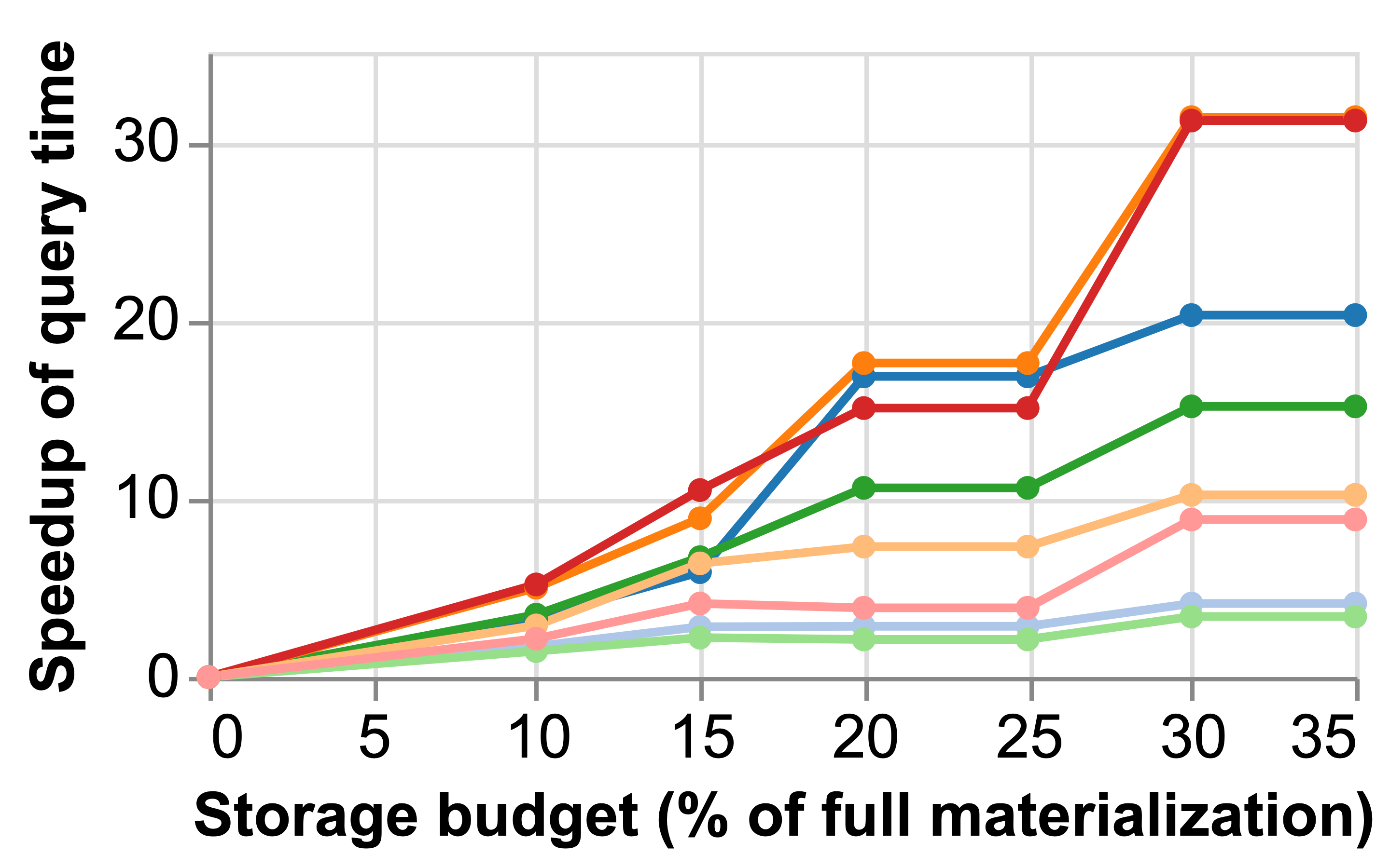
(a) CIFAR10-VGG16

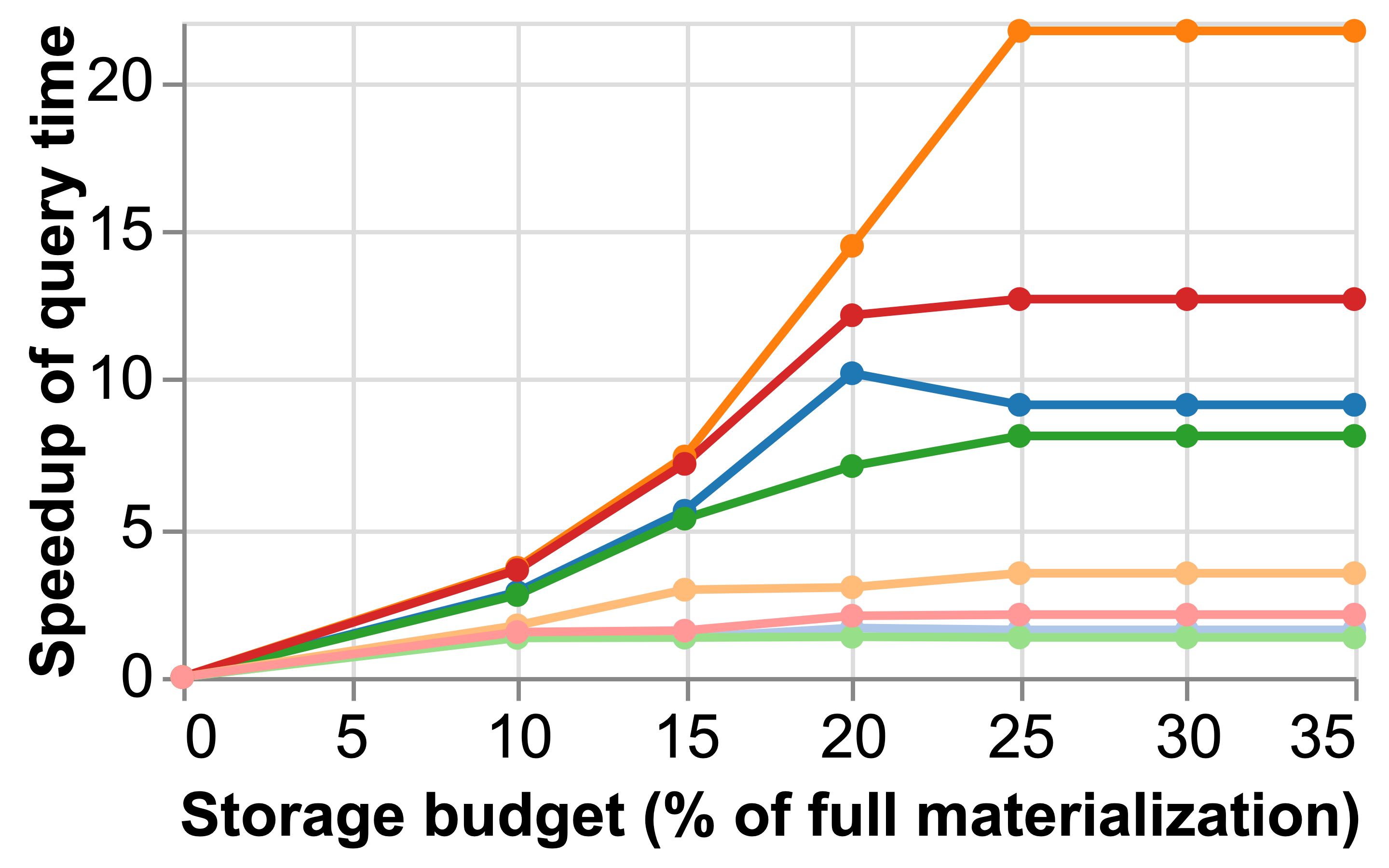
(b) ImageNet-ResNet50

Figure 9. Speedups against ReprocessAll by DeepEverest when given different storage budgets.

5.5. Preprocessing Costs

This experiment evaluates the costs of preprocessing in an extreme case where the user queries all layers in the DNN. Note that with incremental indexing, the costs of index computation and persistence for each layer are incurred once only if that layer is queried. In this experiment, DeepEverest is given a storage budget of $20\%$ of full materialization and preprocesses all layers for each dataset and model from the first layer to the last layer. Convolutional layers, activation layers, and batch normalization layers are considered separate layers. We measure the cumulative times for each component in preprocessing: DNN inference, data persistence (for PreprocessAll, persisting the activations to disk; for DeepEverest, persisting NPI and MAI to disk), and index computation. We force-write the data to disk when measuring the time for data persistence. Figure 10 shows the results. DeepEverest has similar preprocessing times compared with PreprocessAll. The time for building NPI and MAI and persisting them to disk is similar to the time for PreprocessAll to persist the activations to disk. Note that DNN inference takes longer for late layers than for early layers. We also observe that data persistence and index computation for early layers takes longer than for late layers, since the sizes of early layers are usually greater than that of late layers. Considering these results along with the results shown in Section 5.2, DeepEverest achieves comparable and sometimes better query times than PreprocessAll, with only $20\%$ of its storage overhead and similar preprocessing times.

5.6. Effectiveness of IQA

Finally, we evaluate the effectiveness of Inter-Query Acceleration (IQA) for sequences of related queries. We randomly select five inputs and construct two sequences of related queries for each input on various layers. Both sequences consist of $1{,}000$ SimHigh queries. The first query of each sequence targets a RandHigh neuron group containing $n_{size}$ neurons. Each later query randomly replaces $n_{replace}$ neurons in the neuron group of the previous query by $n_{replace}$ randomly selected RandHigh neurons. Sequence 1 sets $n_{size}{=}5$ and $n_{replace}{=}1$. Sequence 2 sets $n_{size}{=}10$ and $n_{replace}{=}2$.

We measure the speedups for query times of DeepEverest with IQA against DeepEverest without IQA for each query. Figure 11 shows the median of the speedups for each query on CIFAR10-VGG16 given an in-memory cache budget of 1 GB for IQA, with $nPartitions{=}16$ and $ratio{=}0$ set for DeepEverest. We observe that even with this small budget, IQA consistently improves DeepEverest’s query times across different layers. Not shown in the paper, we also experiment with different $nPartitions$ and $ratio$ and different cache budgets. We find that IQA always consistently speeds up related queries and larger budgets generally lead to larger speedups. In Figure 11, the speedups for the first query are around $1{\times}$ since the in-memory cache is initially empty. For later queries when the cache is populated, for Sequence 1, DeepEverest with IQA achieves speedups of $2.65{\times}$ to $8.73{\times}$ for the late layer, $3.97{\times}$ to $8.08{\times}$ for the mid layer, and $1.53{\times}$ to $3.38{\times}$ for the early layer. For Sequence 2, DeepEverest with IQA achieves speedups of $4.00{\times}$ to $8.06{\times}$ for the late layer, $4.29{\times}$ to $7.86{\times}$ for the mid layer, and $1.48{\times}$ to $1.82{\times}$ for the early layer. The speedups for the early layer are smaller because this layer is larger, and hence the in-memory cache can hold fewer inputs’ activations of the full layer. We observe larger speedups for the early layer with larger cache budgets.

(a)

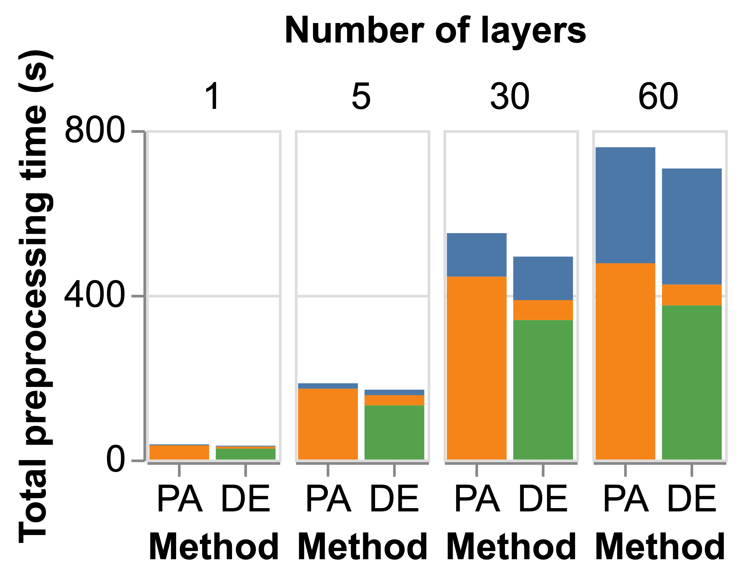
(a) CIFAR10-VGG16

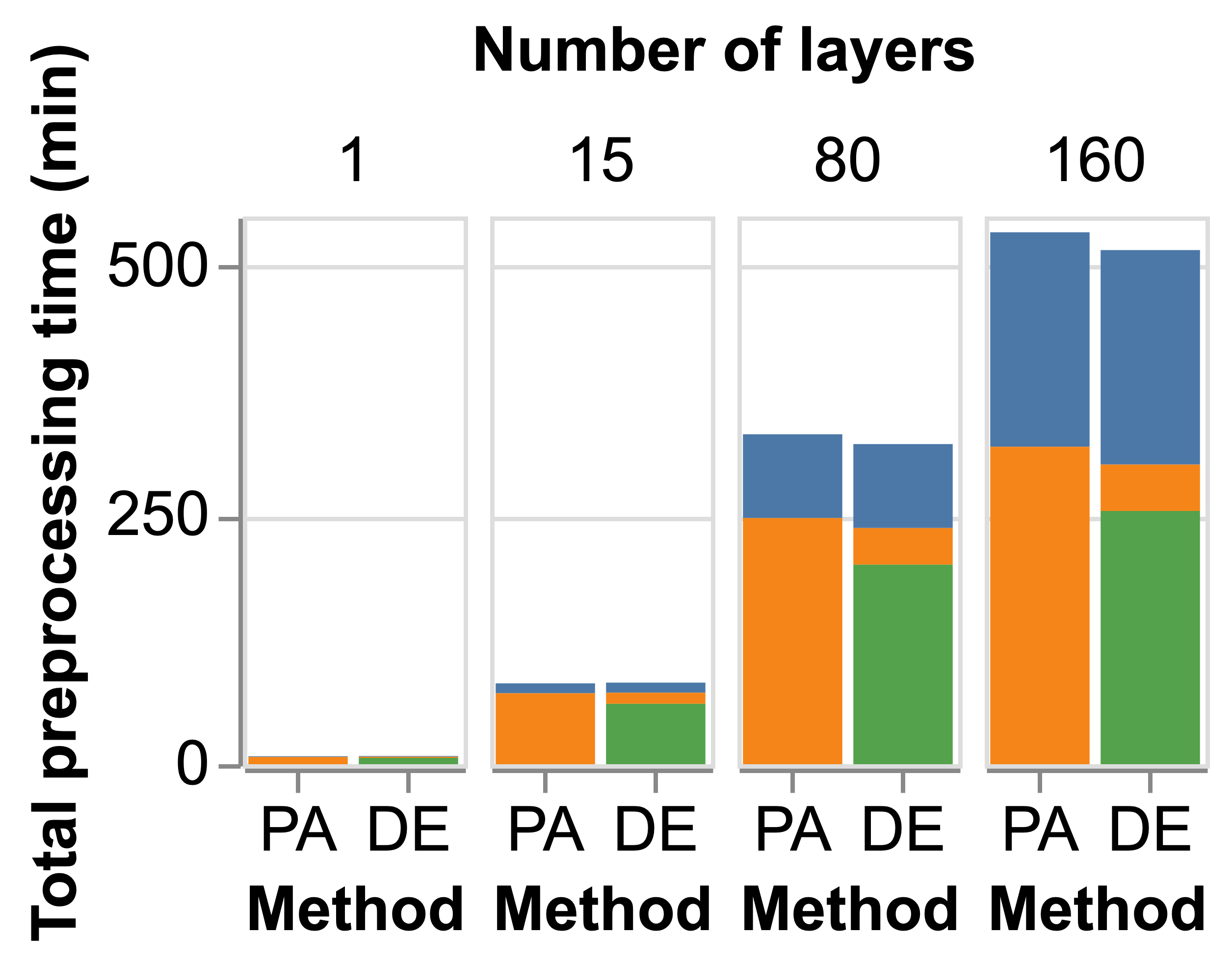
(b) ImageNet-ResNet50

Figure 10. Cumulative preprocessing times from the first layer to the last layer for PreprocessAll and DeepEverest.

(a)

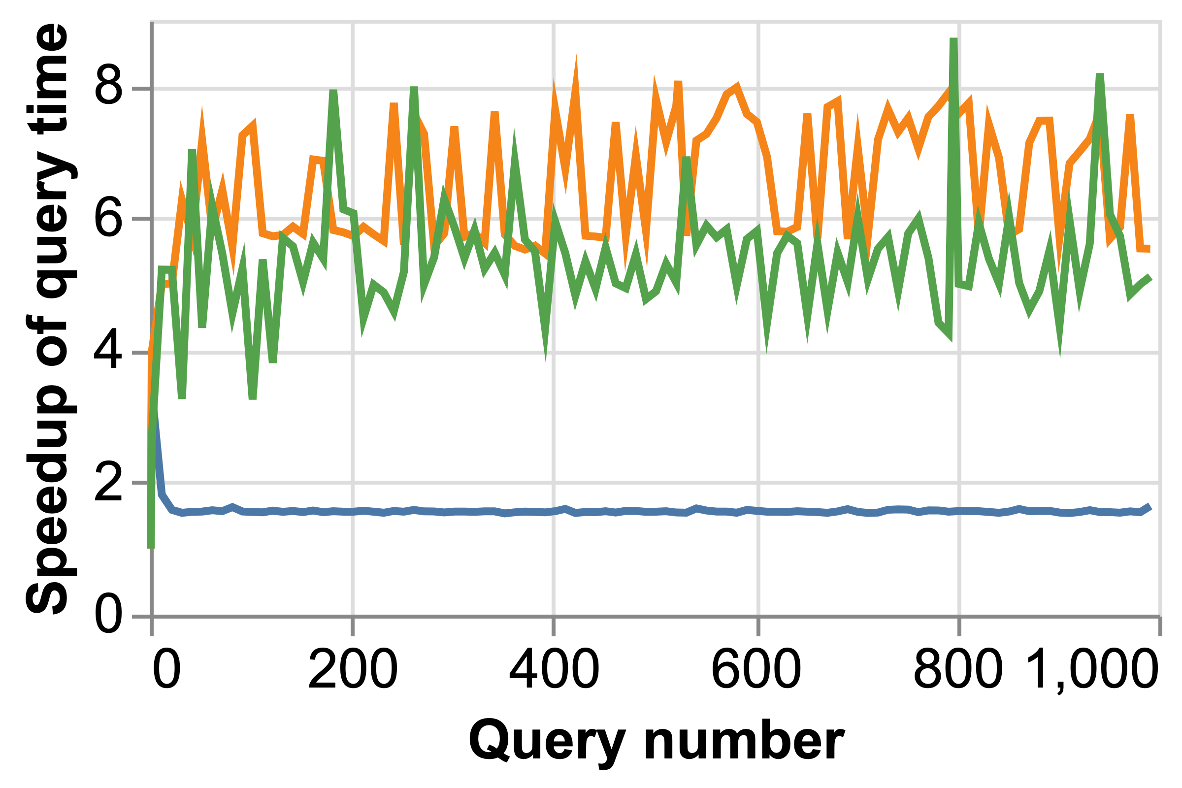
(a) Sequence 1

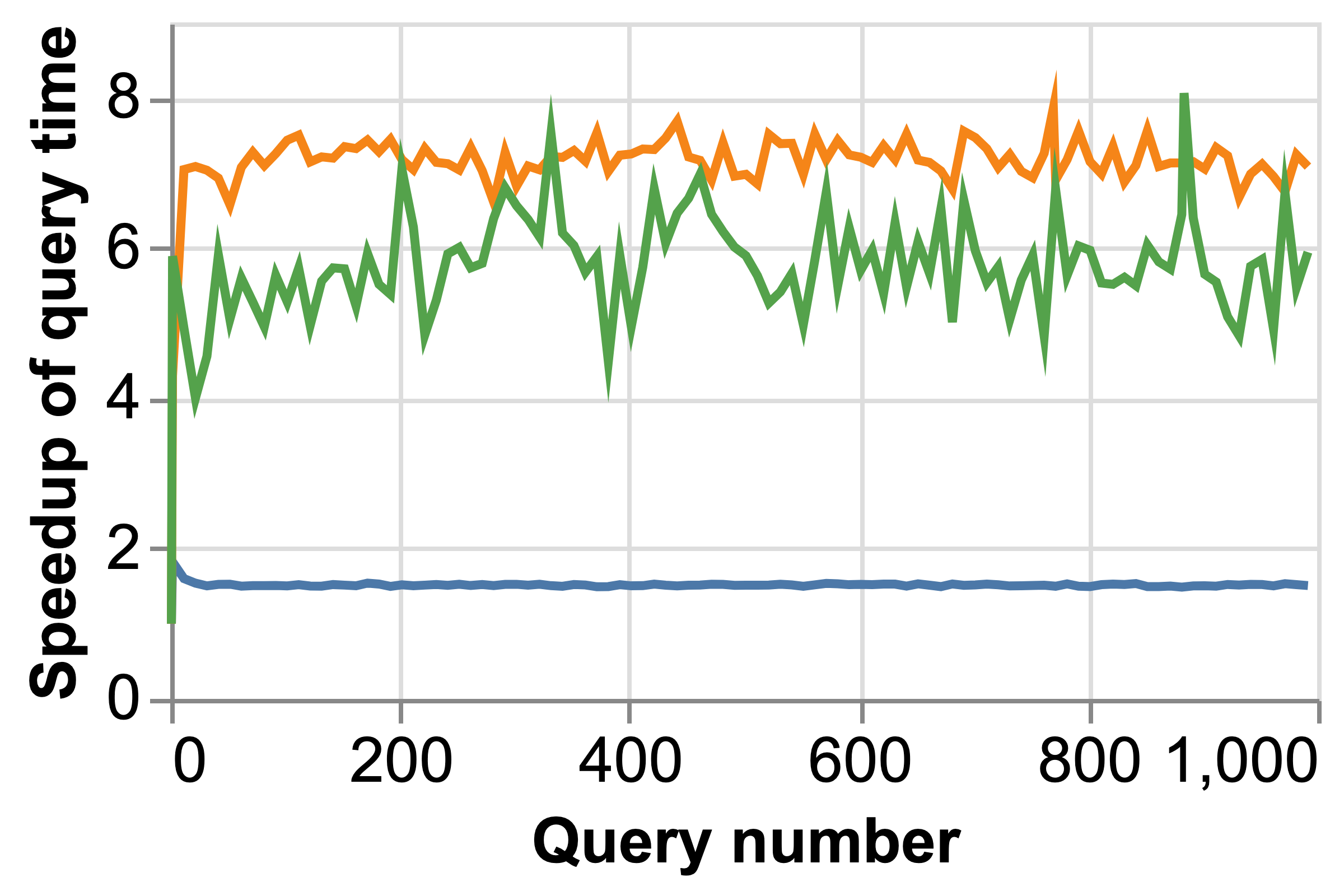
(b) Sequence 2

Figure 11. Speedups of query times by DeepEverest with IQA (1 GB cache budget) against DeepEverest without IQA.

6. Discussion

This section discusses some possible optimizations and extensions for DeepEverest.

Incrementally Returning Query Results. NTA runs until it has found $k$ inputs whose distances to the sample $s$ are at most the threshold value, $t$. However, NTA may be certain that some inputs are part of the top-$k$ set before it has found the complete set. For queries where $k>1$, after each round of the algorithm, DeepEverest returns inputs in $Y\subseteq U$, where for all $y\in Y$, $dist(s,y,G)\leq t$, and continues running to find the rest of the $k-|Y|$ results. DeepEverest’s optimizations enable it to incrementally return the top-$k$ results quickly, and therefore reduces the time required to return the first part of the answer to the user.

Approximation. Modifying DeepEverest to give approximate results is straightforward. Following the definition of the $\theta$-approximation in Fagin’s paper (Fagin et al., 2003), a $\theta$-approximation (let $0<\theta<1$ be given) to the top-$k$ answers is a collection of $k$ inputs, $U$, (and their distances to the sample input) such that for each $y\in U$ and each $z\in D\setminus U$, $\theta*dist(s,y,G)\leq dist(s,z,G)$. Let $t$ be the threshold value from eq. 3. DeepEverest can find a $\theta$-approximation to the top-$k$ answers by modifying the termination condition in eq. 4 to be,

(6) $$\max_{x\in top}\left\{dist(s,x,G)\right\}\leq t/\theta$$

Early Stopping. DeepEverest can be further modified into an interactive process in which it can show the user the current top-$k$ results with a guarantee about the degree of approximation to the correct top-$k$ results. Based on this guarantee, the user can decide whether they would like to stop the process at any time. Let $b$ be the largest distance to the sample input from the current top-$k$ results, let $t$ be the current threshold value, and let $\theta=t/b$. If the algorithm is stopped early, we have $0<\theta<1$ because $b>t$. Therefore, the current top-$k$ results is then a $\theta$-approximation to the correct top-$k$ answers. Thus, the user can be shown the current top-$k$ results and the number $\theta$, with a guarantee that they are being shown a $\theta$-approximation.

7. Conclusion

We presented DeepEverest, a system that accelerates top-$k$ queries for DNN interpretation. DeepEverest, with various optimizations, reduces the number of activations computed at query time with low storage overhead, while guaranteeing correct query results. With less than $20\%$ of the storage of full materialization, DeepEverest accelerates individual queries by up to $63.5{\times}$ and consistently outperforms other methods over various multi-query workloads.

References

- (1)
- Akbarinia et al. (2007) Reza Akbarinia, Esther Pacitti, and Patrick Valduriez. 2007. Best Position Algorithms for Top-K Queries. In Proceedings of the 33rd International Conference on Very Large Data Bases. VLDB Endowment, 495–506.
- Amershi et al. (2015) Saleema Amershi, Max Chickering, Steven M Drucker, Bongshin Lee, Patrice Simard, and Jina Suh. 2015. ModelTracker: Redesigning Performance Analysis Tools for Machine Learning. In Proceedings of the 33rd Annual ACM Conference on Human Factors in Computing Systems. ACM, 337–346.
- Andoni and Indyk (2006) Alexandr Andoni and Piotr Indyk. 2006. Near-Optimal Hashing Algorithms for Approximate Nearest Neighbor in High Dimensions. In 2006 47th Annual IEEE Symposium on Foundations of Computer Science. IEEE, 459–468.
- Bast et al. (2006) Holger Bast, Debapriyo Majumdar, Ralf Schenkel, Martin Theobald, and Gerhard Weikum. 2006. IO-Top-K: Index-Access Optimized Top-K Query Processing. In Proceedings of the 32nd International Conference on Very Large Data Bases. VLDB Endowment, 475–486.
- Bau et al. (2017) David Bau, Bolei Zhou, Aditya Khosla, Aude Oliva, and Antonio Torralba. 2017. Network Dissection: Quantifying Interpretability of Deep Visual Representations. In 2017 IEEE Conference on Computer Vision and Pattern Recognition. IEEE, 6541–6549.
- Bau et al. (2020) David Bau, Jun-Yan Zhu, Hendrik Strobelt, Agata Lapedriza, Bolei Zhou, and Antonio Torralba. 2020. Understanding the Role of Individual Units in a Deep Neural Network. Proceedings of the National Academy of Sciences 117, 48 (2020), 30071–30078.
- Bentley (1975) Jon Louis Bentley. 1975. Multidimensional Binary Search Trees Used for Associative Searching. Commun. ACM 18, 9 (1975), 509–517.
- Callahan et al. (2006) Steven P Callahan, Juliana Freire, Emanuele Santos, Carlos E Scheidegger, Cláudio T Silva, and Huy T Vo. 2006. VisTrails: Visualization Meets Data Management. In Proceedings of the 2006 ACM SIGMOD International Conference on Management of Data. ACM, 745–747.
- Caruana et al. (1999) Rich Caruana, Hooshang Kangarloo, John David Dionisio, Usha Sinha, and David Johnson. 1999. Case-Based Explanation of Non-Case-Based Learning Methods. In Proceedings of the AMIA Symposium. AMIA, 212.
- Datar et al. (2004) Mayur Datar, Nicole Immorlica, Piotr Indyk, and Vahab S Mirrokni. 2004. Locality-Sensitive Hashing Scheme Based on p-Stable Distributions. In Proceedings of the Twentieth Annual Symposium on Computational Geometry. ACM, 253–262.
- Fagin et al. (2003) Ronald Fagin, Amnon Lotem, and Moni Naor. 2003. Optimal Aggregation Algorithms for Middleware. J. Comput. System Sci. 66, 4 (2003), 614–656.
- Girshick et al. (2014) Ross Girshick, Jeff Donahue, Trevor Darrell, and Jitendra Malik. 2014. Rich Feature Hierarchies for Accurate Object Detection and Semantic Segmentation. In 2014 IEEE Conference on Computer Vision and Pattern Recognition. IEEE, 580–587.
- Gonzalez-Garcia et al. (2018) Abel Gonzalez-Garcia, Davide Modolo, and Vittorio Ferrari. 2018. Do Semantic Parts Emerge in Convolutional Neural Networks? International Journal of Computer Vision 126, 5 (2018), 476–494.
- Goodfellow et al. (2009) Ian J. Goodfellow, Quoc V. Le, Andrew M. Saxe, Honglak Lee, and Andrew Y. Ng. 2009. Measuring Invariances in Deep Networks. In Proceedings of the 22nd International Conference on Neural Information Processing Systems. Curran Associates Inc., 646–654.
- Guttman (1984) Antonin Guttman. 1984. R-Trees: A Dynamic Index Structure for Spatial Searching. ACM SIGMOD Record 14, 2 (1984), 47–57.
- Han et al. (2015) Xixian Han, Jianzhong Li, and Hong Gao. 2015. Efficient Top-K Retrieval on Massive Data. IEEE Transactions on Knowledge and Data Engineering 27, 10 (2015), 2687–2699.
- He et al. (2016) Kaiming He, Xiangyu Zhang, Shaoqing Ren, and Jian Sun. 2016. Deep Residual Learning for Image Recognition. In 2016 IEEE Conference on Computer Vision and Pattern Recognition. IEEE, 770–778.
- Ilyas et al. (2002) Ihab F Ilyas, Walid G Aref, and Ahmed K Elmagarmid. 2002. Joining Ranked Inputs in Practice. In Proceedings of the 28th International Conference on Very Large Data Bases. Elsevier, 950–961.
- Jegou et al. (2010) Herve Jegou, Matthijs Douze, and Cordelia Schmid. 2010. Product Quantization for Nearest Neighbor Search. IEEE Transactions on Pattern Analysis and Machine Intelligence 33, 1 (2010), 117–128.
- Johnson et al. (2019) Jeff Johnson, Matthijs Douze, and Hervé Jégou. 2019. Billion-Scale Similarity Search With GPUs. IEEE Transactions on Big Data (2019).
- Kahng et al. (2017) Minsuk Kahng, Pierre Y Andrews, Aditya Kalro, and Duen Horng Polo Chau. 2017. ActiVis: Visual Exploration of Industry-Scale Deep Neural Network Models. IEEE Transactions on Visualization and Computer Graphics 24, 1 (2017), 88–97.
- Kahng et al. (2016) Minsuk Kahng, Dezhi Fang, and Duen Horng Chau. 2016. Visual Exploration of Machine Learning Results Using Data Cube Analysis. In Proceedings of the Workshop on Human-In-the-Loop Data Analytics. ACM, 1–6.
- Karpathy et al. (2015) Andrej Karpathy, Justin Johnson, and Li Fei-Fei. 2015. Visualizing and Understanding Recurrent Networks. arXiv preprint arXiv:1506.02078 (2015).
- Krause et al. (2016) Josua Krause, Adam Perer, and Kenney Ng. 2016. Interacting with Predictions: Visual Inspection of Black-Box Machine Learning Models. In Proceedings of the 2016 CHI Conference on Human Factors in Computing Systems. ACM, 5686–5697.
- Krishnan and Wu (2017) Sanjay Krishnan and Eugene Wu. 2017. PALM: Machine Learning Explanations for Iterative Debugging. In Proceedings of the 2nd Workshop on Human-In-the-Loop Data Analytics. ACM, 1–6.
- Krizhevsky et al. (2009) Alex Krizhevsky, Geoffrey Hinton, et al. 2009. Learning Multiple Layers of Features From Tiny Images. (2009).
- Kulesza et al. (2015) Todd Kulesza, Margaret Burnett, Weng-Keen Wong, and Simone Stumpf. 2015. Principles of Explanatory Debugging to Personalize Interactive Machine Learning. In Proceedings of the 20th International Conference on Intelligent User Interfaces. ACM, 126–137.
- Lipton (2018) Zachary C Lipton. 2018. The Mythos of Model Interpretability. Queue 16, 3 (2018), 31–57.
- Liu et al. (2016) Mengchen Liu, Jiaxin Shi, Zhen Li, Chongxuan Li, Jun Zhu, and Shixia Liu. 2016. Towards Better Analysis of Deep Convolutional Neural Networks. IEEE Transactions on Visualization and Computer Graphics 23, 1 (2016), 91–100.
- Liu and Deng (2015) Shuying Liu and Weihong Deng. 2015. Very Deep Convolutional Neural Network Based Image Classification Using Small Training Sample Size. In 2015 3rd IAPR Asian Conference on Pattern Recognition (ACPR). IEEE, 730–734.
- Liu et al. (2006) Ting Liu, Andrew W Moore, and Alexander Gray. 2006. New Algorithms for Efficient High-Dimensional Nonparametric Classification. Journal of Machine Learning Research 7 (2006), 1135–1158.
- Ludäscher et al. (2006) Bertram Ludäscher, Ilkay Altintas, Chad Berkley, Dan Higgins, Efrat Jaeger, Matthew Jones, Edward A Lee, Jing Tao, and Yang Zhao. 2006. Scientific Workflow Management and the Kepler System. Concurrency and Computation: Practice and Experience 18, 10 (2006), 1039–1065.
- Ma et al. (2016) Minghuang Ma, Haoqi Fan, and Kris M Kitani. 2016. Going Deeper into First-Person Activity Recognition. In Proceedings of the IEEE Conference on Computer Vision and Pattern Recognition. IEEE, 1894–1903.
- Mehta et al. (2020) Parmita Mehta, Stephen Portillo, Magdalena Balazinska, and Andrew J. Connolly. 2020. Toward Sampling for Deep Learning Model Diagnosis. In 2020 IEEE 36th International Conference on Data Engineering. IEEE, 1910–1913.
- Miao et al. (2017) Hui Miao, Ang Li, Larry S Davis, and Amol Deshpande. 2017. ModelHub: Deep Learning Lifecycle Management. In 2017 IEEE 33rd International Conference on Data Engineering. IEEE, 1393–1394.
- Mikolov et al. (2013) Tomas Mikolov, Ilya Sutskever, Kai Chen, Greg S Corrado, and Jeff Dean. 2013. Distributed Representations of Words and Phrases and their Compositionality. In Proceedings of the 26th International Conference on Neural Information Processing Systems - Volume 2, Vol. 26. Curran Associates Inc., 3111–3119.
- Molnar (2019) Christoph Molnar. 2019. Interpretable Machine Learning. https://christophm.github.io/interpretable-ml-book/.
- Nguyen et al. (2016) Anh Nguyen, Alexey Dosovitskiy, Jason Yosinski, Thomas Brox, and Jeff Clune. 2016. Synthesizing the Preferred Inputs for Neurons in Neural Networks via Deep Generator Networks. In Proceedings of the 30th International Conference on Neural Information Processing Systems. Curran Associates Inc., 3387–3395.
- NVIDIA ([n.d.]) NVIDIA. [n.d.]. NVIDIA Data Center Deep Learning Product Performance. https://developer.nvidia.com/deep-learning-performance-training-inference.
- Olah et al. (2018) Chris Olah, Arvind Satyanarayan, Ian Johnson, Shan Carter, Ludwig Schubert, Katherine Ye, and Alexander Mordvintsev. 2018. The Building Blocks of Interpretability. Distill 3, 3 (2018), e10.
- Omohundro (1989) Stephen M Omohundro. 1989. Five Balltree Construction Algorithms. International Computer Science Institute Berkeley.
- Pang et al. (2010) HweeHwa Pang, Xuhua Ding, and Baihua Zheng. 2010. Efficient Processing of Exact Top-K Queries over Disk-Resident Sorted Lists. The VLDB Journal 19, 3 (2010), 437–456.
- Papernot and McDaniel (2018) Nicolas Papernot and Patrick McDaniel. 2018. Deep K-Nearest Neighbors: Towards Confident, Interpretable and Robust Deep Learning. arXiv preprint arXiv:1803.04765 (2018).
- Ribeiro et al. (2016) Marco Tulio Ribeiro, Sameer Singh, and Carlos Guestrin. 2016. “Why Should I Trust You?”: Explaining the Predictions of Any Classifier. In Proceedings of the 22nd ACM SIGKDD International Conference on Knowledge Discovery and Data Mining. ACM, 1135–1144.
- Russakovsky et al. (2015) Olga Russakovsky, Jia Deng, Hao Su, Jonathan Krause, Sanjeev Satheesh, Sean Ma, Zhiheng Huang, Andrej Karpathy, Aditya Khosla, Michael Bernstein, et al. 2015. ImageNet Large Scale Visual Recognition Challenge. International Journal of Computer Vision 115, 3 (2015), 211–252.
- Sellam et al. (2019) Thibault Sellam, Kevin Lin, Ian Huang, Michelle Yang, Carl Vondrick, and Eugene Wu. 2019. DeepBase: Deep Inspection of Neural Networks. In Proceedings of the 2019 International Conference on Management of Data. ACM, 1117–1134.
- Simonyan and Zisserman (2014) Karen Simonyan and Andrew Zisserman. 2014. Very Deep Convolutional Networks for Large-Scale Image Recognition. arXiv preprint arXiv:1409.1556 (2014).
- Sparks et al. (2017) E. R. Sparks, S. Venkataraman, T. Kaftan, M. J. Franklin, and B. Recht. 2017. KeystoneML: Optimizing Pipelines for Large-Scale Advanced Analytics. In 2017 IEEE 33rd International Conference on Data Engineering. IEEE, 535–546.
- Srivastava et al. (2013) Rupesh Kumar Srivastava, Jonathan Masci, Sohrob Kazerounian, Faustino Gomez, and Jürgen Schmidhuber. 2013. Compete to Compute. In Proceedings of the 26th International Conference on Neural Information Processing Systems - Volume 2. Curran Associates Inc., 2310–2318.
- Szegedy et al. (2013) Christian Szegedy, Wojciech Zaremba, Ilya Sutskever, Joan Bruna, Dumitru Erhan, Ian Goodfellow, and Rob Fergus. 2013. Intriguing Properties of Neural Networks. arXiv preprint arXiv:1312.6199 (2013).
- Theobald et al. (2004) Martin Theobald, Gerhard Weikum, and Ralf Schenkel. 2004. Top-K Query Evaluation With Probabilistic Guarantees. In Proceedings of the Thirtieth International Conference on Very Large Data Bases. VLDB Endowment, 648–659.
- Vartak et al. (2018) Manasi Vartak, Joana M F. da Trindade, Samuel Madden, and Matei Zaharia. 2018. MISTIQUE: A System to Store and Query Model Intermediates for Model Diagnosis. In Proceedings of the 2018 International Conference on Management of Data. ACM, 1285–1300.
- Vartak et al. (2016) Manasi Vartak, Harihar Subramanyam, Wei-En Lee, Srinidhi Viswanathan, Saadiyah Husnoo, Samuel Madden, and Matei Zaharia. 2016. MODELDB: A System for Machine Learning Model Management. In Proceedings of the Workshop on Human-In-the-Loop Data Analytics. ACM, 1–3.
- Wallace et al. (2018) Eric Wallace, Shi Feng, and Jordan Boyd-Graber. 2018. Interpreting Neural Networks With Nearest Neighbors. arXiv preprint arXiv:1809.02847 (2018).
- Weiss et al. (2009) Yair Weiss, Antonio Torralba, and Rob Fergus. 2009. Spectral Hashing. In Proceedings of the 21st International Conference on Neural Information Processing Systems, Vol. 21. Curran Associates, Inc.
- Xin et al. (2018) Doris Xin, Stephen Macke, Litian Ma, Jialin Liu, Shuchen Song, and Aditya Parameswaran. 2018. HELIX: Holistic Optimization for Accelerating Iterative Machine Learning. Proceedings of the VLDB Endowment 12, 4 (2018), 446–460.
- Yosinski et al. (2015) Jason Yosinski, Jeff Clune, Anh Nguyen, Thomas Fuchs, and Hod Lipson. 2015. Understanding Neural Networks Through Deep Visualization. arXiv preprint arXiv:1506.06579 (2015).
- Zeiler and Fergus (2014) Matthew D. Zeiler and R. Fergus. 2014. Visualizing and Understanding Convolutional Networks. In Computer Vision – ECCV 2014. Springer, 818–833.
- Zhang et al. (2016) Shile Zhang, Chao Sun, and Zhenying He. 2016. Listmerge: Accelerating Top-K Aggregation Queries Over Large Number of Lists. In International Conference on Database Systems for Advanced Applications. Springer, 67–81.
- Zhou et al. (2018a) Bolei Zhou, David Bau, Aude Oliva, and Antonio Torralba. 2018a. Interpreting Deep Visual Representations via Network Dissection. IEEE Transactions on Pattern Analysis and Machine Intelligence 41, 9 (2018), 2131–2145.
- Zhou et al. (2014) Bolei Zhou, Aditya Khosla, Agata Lapedriza, Aude Oliva, and Antonio Torralba. 2014. Object Detectors Emerge in Deep Scene CNNs. arXiv preprint arXiv:1412.6856 (2014).
- Zhou et al. (2018b) Bolei Zhou, Yiyou Sun, David Bau, and Antonio Torralba. 2018b. Revisiting the Importance of Individual Units in CNNs via Ablation. arXiv preprint arXiv:1806.02891 (2018).