Learning Optical Flow from a Few Matches

Abstract

State-of-the-art neural network models for optical flow estimation require a dense correlation volume at high resolutions for representing per-pixel displacement. Although the dense correlation volume is informative for accurate estimation, its heavy computation and memory usage hinders the efficient training and deployment of the models. In this paper, we show that the dense correlation volume representation is redundant and accurate flow estimation can be achieved with only a fraction of elements in it. Based on this observation, we propose an alternative displacement representation, named Sparse Correlation Volume, which is constructed directly by computing the k closest matches in one feature map for each feature vector in the other feature map and stored in a sparse data structure. Experiments show that our method can reduce computational cost and memory use significantly, while maintaining high accuracy compared to previous approaches with dense correlation volumes. Code is available at https://github.com/zacjiang/scv.

1 Introduction

(a) First image

(b) Second image

(c) Dense correlation volume

(d) Sparse correlation volume

(e) Optical flow (RAFT [29])

(f) Optical flow (ours)

Figure 1: Optical flow estimation with dense correlation volume and sparse correlation volume. (c) and (d) illustrate the correlation volumes for a single pixel (yellow dot) in the first image. The white crosses in (b) indicate the top-$k$ matches. We show accurate optical flow can be estimated given only a few matching correlations.

(a) A dense correlation volume requires saving all pairs of matches.

(b) A sparse correlation volume requires saving only top-$k$ matches.

Figure 2: Comparison between dense correlation volume and top-$k$ sparse correlation volume. In a sparse correlation volume, only the top-$k$ matches are stored and the rest are discarded.

Optical flow estimation is a classic problem in computer vision [11]. It aims at finding pixelwise correspondences between two images. Traditionally it has been formulated as an optimization problem solved by continuous [4, 11, 32] or discrete [22, 7, 31] optimization. Since the development of deep learning, optical flow estimation has been formulated as a learning problem where direct regression from a neural network becomes a common approach [9, 16].

One popular representation in dense correspondence problems is the correlation (cost) volume, first introduced by Hosni et al.[12]. Correlation volumes give an explicit representation of per-pixel displacements and have demonstrated their wide use in learning problems of stereo matching [18] and optical flow [9, 27]. Contrary to stereo matching problems, where the search space is along a scanline, optical flow problems have a 2D search space, which leads to two challenges: large memory consumption and high computational cost when directly processing a 4D volume.

To reduce the memory and computational cost, existing approaches [27, 34, 33, 13, 36] first build a feature pyramid and compute correlation volumes at coarse resolutions, then gradually warp upper-level feature maps based on up-sampled flow and construct a local correlation volume over a limited search range. One notable problem observed in previous work [4, 32, 20], was that coarse-to-fine frameworks fail to address the case when the flow displacement is larger than the flow structure, i.e. the famous small objects moving fast problem.

Recent approaches, Devon and RAFT [20, 29] proposed using direct search in the second image to remove the need for warping. RAFT especially demonstrated the benefit of first constructing an all-pairs correlation volume and directly processing it at a single resolution rather than in a coarse-to-fine manner. However, the all-pairs correlation volume requires pair-wise dot product between the two feature maps. Hence, both the time and the space complexity are $O(N^{2})$, where $N$ is the number of pixels of an image. A small $N$ is required to reduce the memory consumption and therefore RAFT can only use $1/8$ resolution feature maps. A low-resolution feature map cannot fully represent the fine details of an image. We wonder if there is a way to construct a correlation volume with the all-pairs search range but without exceeding the maximum GPU memory. We thus question the necessity of storing all pairwise correlations and hypothesize that only storing the top-$k$ correlations for each pixel might be sufficient.

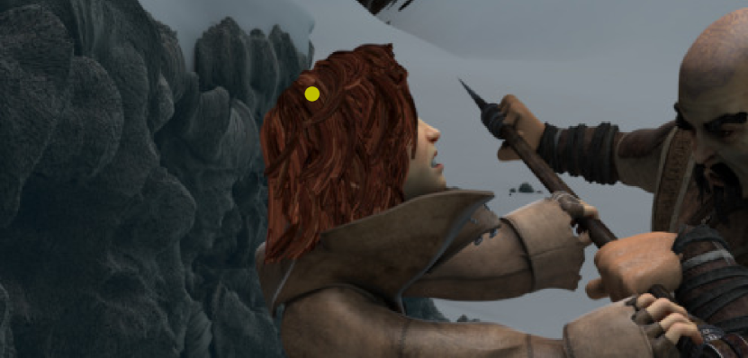
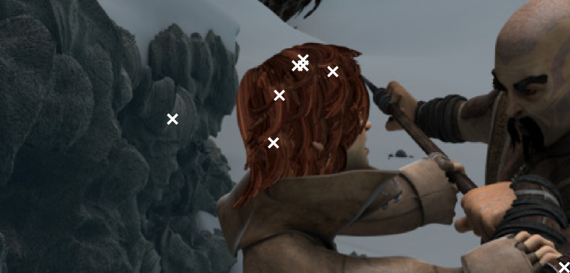
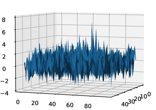
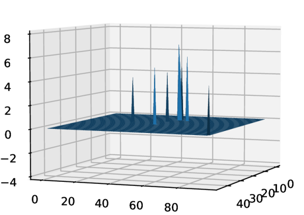
Our intuition is that a feature vector in one image has only a few feature vectors in the other image with high correlation to match. Hence, there could be large redundancy in the dense correlation volume where the small correlations do not contribute to the prediction. Figure 1 illustrates the comparison between a dense correlation volume and a sparse correlation volume.

We propose a Sparse Correlation Volume representation, where only the top-$k$ correlations for each pixel are stored in a sparse data structure defined by a {value, coordinates} pair. In this paper, we demonstrate how a sparse correlation volume representation can be used to solve the optical flow problem. We propose an approach to construct and process such a sparse correlation volume in an optical flow learning framework. We demonstrate that even if only a small fraction of elements are stored, our results are still comparable to previous work [29] which employs a dense correlation volume. We finally demonstrate that the sparse approach allows the construction of a high-resolution correlation volume, which can predict the motions of fine structures more accurately than previous approaches.

Figure 3: Network architecture and residual flow prediction for a single iteration. (1) $F_{1}$ and $F_{2}$ are feature maps extracted by a feature extraction network. We form the 4D sparse correlation volume by first computing a set of displacements ${\mathbf{d}}_{0}\in\widetilde{\mathcal{K}}$ with top-$k$ correlations with KNN. We then take the dot product for each feature vector in $F_{1}$ with its $k$ corresponding feature vectors in $F_{2}$. The dashed arrows denote paths that have no gradient flow while the solid arrows denote paths that do. (2) In each iteration, the displacement vectors are updated by subtracting the residual flow ${\mathbf{d}}_{i}-\Delta{\mathbf{f}}_{i}$ to update the 4D correlation volume. A multi-scale displacement encoder is applied to encode the 4D sparse correlation volume to a 2D dense motion tensor. (3) A GRU update block is applied to predict the residual flow $\Delta{\mathbf{f}}_{i+1}$ for the next iteration. The GRU block also takes input of ${\mathbf{h}}_{i},F_{c},{\mathbf{f}}_{i}$ which represents the hidden state vector of current iteration, feature map extracted by the context network and current estimation of optical flow, and outputs the hidden state vector for the next iteration as well the residual flow.

2 Method

Let $I_{1},I_{2}:{\mathbb{Z}}^{2}\rightarrow\mathbb{R}^{3}$ be two RGB images. The problem is to estimate a dense flow field ${\mathbf{f}}:{\mathbb{Z}}^{2}\rightarrow\mathbb{R}^{2}$ that maps each pixel coordinate ${\mathbf{x}}$ to a displacement vector ${\mathbf{f}}({\mathbf{x}})$.

In modern deep learning optical flow approaches, a feature extraction network is first applied to extract feature maps from the image pair, $F_{1},F_{2}:{\mathbb{Z}}^{2}\rightarrow\mathbb{R}^{c}$, where $c$ is the number of channels. The correlation volume $C:{\mathbb{Z}}^{4}\rightarrow\mathbb{R}$ is formed by computing inner products between pairwise feature vectors,

$$C({\mathbf{x}},{\mathbf{d}})=F_{1}({\mathbf{x}})\cdot F_{2}({\mathbf{x}}+{\mathbf{d}}).$$ (1)

The output is a four-dimensional tensor which can be represented as a set

$$\mathcal{C}=\{C({\mathbf{x}},{\mathbf{d}})\;|\;{\mathbf{x}}\in\mathcal{X},{\mathbf{d}}\in\mathcal{D}\}.$$ (2)

Here, ${\mathcal{X}=[0,h)\times[0,w)\cap{\mathbb{Z}}^{2}}$ is the domain of the feature map $F_{1}$ and ${|\mathcal{X}|=hw}$, where $h$ and $w$ represent the height and width of $F_{1}$ respectively. The displacement set $\mathcal{D}$ is defined as ${\mathcal{D}=[-d,d]^{2}\cap{\mathbb{Z}}^{2}}$ where $d$ represents the maximum displacement along the $x$ or $y$ direction and ${|\mathcal{D}|=(2d+1)^{2}}$. Therefore, the correlation volume $\mathcal{C}$ contains ${hw(2d+1)^{2}}$ elements.

To reduce the size of the correlation volume, previous approaches use coarse-to-fine and warping methods to constrain the size of $d$ [27, 13, 33]. To handle large displacements accurately, RAFT [29] constructs an all-pairs correlation volume where the displacement range contains the entire feature map. Excluding out-of-range matches, RAFT’s all-pairs correlation volume contains $N^{2}$ elements where $N=hw$. Therefore, lower-resolution feature maps are required to constrain $N$. In this work, we show that the all-pairs correlation volume can in fact be a sparse tensor, where only a small fraction of the values are stored and processed. We show that we can effectively reduce the spatial complexity from $O(N^{2})$ to $O(Nk)$ with only a minor drop of performance, where $k$ gives the number of matches we want to keep. The main idea is demonstrated in Figure 2.

2.1 Sparse Correlation Volume

For each ${\mathbf{x}}\in\mathcal{X}$, we define a set

$$S_{\mathbf{x}}^{(k)}=\operatorname*{arg\,max}_{S\subset\mathcal{D},|S|=k}\sum_{{\mathbf{d}}\in S}C({\mathbf{x}},{\mathbf{d}})$$ (3)

containing the $k$ displacements that give the maximum correlations. The correlation volume can now be represented as a four-dimensional sparse tensor

$$\widetilde{\mathcal{C}}=\{C({\mathbf{x}},{\mathbf{d}})\;|\;{\mathbf{d}}\in S_{\mathbf{x}}^{(k)},{\mathbf{x}}\in\mathcal{X}\}.$$ (4)

This sparse correlation volume contains ${hwk}$ elements as opposed to the original dense correlation volume with ${h^{2}w^{2}}$ elements. The constant $k$ is typically a small number (e.g. $k=8$).

We now show how to construct the sparse correlation volume and estimate optical flow from it. Our network architecture is shown in Figure 3.

2.2 $k$-Nearest Neighbours

We first use two weight-sharing feature extraction networks to extract $1/4$ resolution feature maps from the input images. Our feature extraction networks consist of six residual blocks and the number of feature channels is $256$. To construct the sparse correlation volume, we use a $k$-nearest neighbours ($k$NN) module [17] to compute a set of indices with the $k$ largest correlation scores for each feature vector in $F_{1}$. The sparse correlation volume is computed by taking the dot product between each feature vector in $F_{1}$ with the top $k$ feature vectors given by the indices in $F_{2}$. During back-propagation, the gradients are only propagated to the $k$ feature vectors that are selected by the $k$NN module.

(a) Displacements update. As a pixel’s coordinates are updated by adding $\Delta\mathbf{f}_{i}$, the relative displacements are diminished by $\Delta\mathbf{f}_{i}$.

(b) Multi-scale displacement encoder. We first form a multi-level sparse correlation pyramid by scaling the coordinates by different constants. We then bilinearly splat the correlations onto the integer grids and extract correlation values within a local window. The extracted windows are converted to dense tensors and are reshaped and concatenated to form a single $h\times w\times c$ tensor.

Figure 4: Illustration of how to process a sparse correlation volume in an iterative fashion.

2.3 Displacements Update

We adopt an overall iterative residual refinement approach. As shown by previous work [15, 29], estimating residual flows can effectively reduce the search space and predict better results than direct regression [16, 9]. Rather than directly predicting optical flow ${\mathbf{f}}$, a residual flow $\Delta{\mathbf{f}}_{i+1}$ is predicted at each step and used to update the current flow estimation ${\mathbf{f}}_{i+1}={\mathbf{f}}_{i}+\Delta{\mathbf{f}}_{i+1}$.

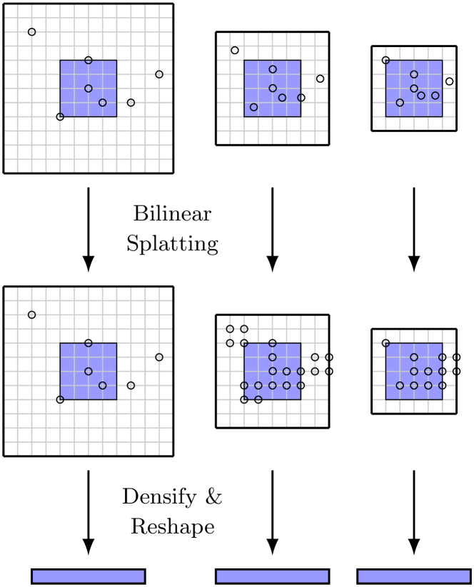
At each step, a pixel ${\mathbf{x}}$ in $F_{1}$ is mapped to ${\mathbf{x}}_{i}$ in $F_{2}$ according to the current estimate of flow ${\mathbf{x}}_{i}={\mathbf{x}}+{\mathbf{f}}_{i}$. Our sparse correlation volume $\widetilde{\mathcal{C}}$ described in Section 2.1 can be regarded as an initial estimation ${\mathbf{f}}_{0}=0$ at $i=0$. When the coordinate ${\mathbf{x}}_{i}$ is updated to ${\mathbf{x}}_{i+1}={\mathbf{x}}_{i}+\Delta{\mathbf{f}}_{i}$, the relative displacements in $\widetilde{\mathcal{C}}$ should be updated accordingly as well. To do so, we shift the coordinates of the sparse correlation tensor by subtracting $k$-nearest neighbouring $\Delta{\mathbf{f}}_{i}$ from ${\mathbf{d}}_{i}$ in each step, $C_{i}({\mathbf{x}},{\mathbf{d}}_{i})=C_{i+1}({\mathbf{x}},{\mathbf{d}}_{i}-\Delta{\mathbf{f}}_{i})$, as depicted in Figure 4(a). Note here we allow ${\mathbf{d}}_{i}-\Delta{\mathbf{f}}_{i}$ to be floating-point. It is also important to note that the inner products are computed only once at the start since in each step, only the correlation coordinates change while the correlation values remain the same.

2.4 Multi-scale Displacement Encoder

One question that is often raised with any sparse approach is how to process a sparse tensor, since the regularity of a normal dense $h\times w\times c$ tensor is lost. Sparse convolutions [8] may be used, however, we will present a simpler and more efficient approach here.

A dense all-pairs correlation volume has dimension $h\times w\times h\times w$ and we have reduced it to a sparse tensor with $h\times w\times k$ elements where only the top-$k$ correlations for each pixel are saved. We can see that the first two dimensions are still dense and what has become sparse are the third and fourth dimensions. The goal here is to encode the $k$ elements for each pixel and form a dense $h\times w\times c$ tensor, which can later be used to predict $\Delta{\mathbf{f}}_{i+1}$.

Following previous work [29], we propose creating multi-scale sparse tensors and sampling displacements locally with a fixed radius at different resolutions. Coarser resolutions give larger context while finer resolutions give more accurate displacements. We then convert the sparse tensors at each level to dense tensors and concatenate them to form a single 2D tensor. This is illustrated in Figure 4(b).

At each iteration $i$, for each pixel ${\mathbf{x}}$, we start with a set of the top $k$ correlation positions $S_{\mathbf{x}}^{(k)}$. So, the set $\{\big{(}{\mathbf{d}},C({\mathbf{x}},{\mathbf{d}})\big{)}~{}|~{}{\mathbf{d}}\in S_{\mathbf{x}}^{(k)}\}$ records the top $k$ correlation values for pixel ${\mathbf{x}}$ and their locations, obtained using a $k$NN algorithm.

We construct a five-level sparse correlation volume pyramid by dividing the coordinates by $(1,2,4,8,16)$ and denote the scaled displacements at level $l$, updated with the current $\Delta{\mathbf{f}}_{i}$ by ${\mathbf{d}}^{l}=\left({\mathbf{d}}_{i}-\Delta{\mathbf{f}}_{i}\right)~{}/~{}2^{l-1}$.

In addition, we denote the correlation values at level $l$ by $C^{l}({\mathbf{x}},{\mathbf{d}}^{l})=C({\mathbf{x}},{\mathbf{d}})$ for ${\mathbf{d}}\in S_{\mathbf{x}}^{(k)}$. At each level, we constrain the displacements by a constant radius $r$ and define the windowed set of correlation values at level $l$,

$$\big{\{}\big{(}{\mathbf{d}}^{l},C^{l}({\mathbf{x}},{\mathbf{d}}^{l})\big{)}~{}\big{|}~{}\|{\mathbf{d}}^{l}\|_{\infty}\leq r,\,{\mathbf{d}}\in S_{\mathbf{x}}^{(k)}\big{\}}~{}.$$ (5)

Since the coordinates ${\mathbf{d}}^{l}$ are not necessarily integers, we need to resample to integer coordinates in order to densify the sparse tensor of correlations. We propose an approach which we call “bilinear splatting”. The correlation values are bilinearly splatted to the four nearest integer grids. For instance, the correlation $C^{l}({\mathbf{x}},{\mathbf{d}}^{l})$ at location ${\mathbf{d}}^{l}$ is propagated to each of four neighbouring integer points, denoted by $[{\mathbf{d}}^{l}]=(d_{x},d_{y})$, according to

$$C^{l}({\mathbf{x}},[{\mathbf{d}}^{l}])=\left(1-|d_{x}^{l}-d_{x}|\right)\left(1-|d_{y}^{l}-d_{y}|\right)C^{l}({\mathbf{x}},{\mathbf{d}}^{l}).$$

These values are then summed for the set of correlations (5) and the sparse tensors of each level are converted to dense tensors, reshaped and concatenated to form a single 2D dense tensor of dimension $5(2r+1)^{2}$, where $5$ is the number of pyramid levels.

The approach we introduce here does not require learning. It is merely a conversion between sparse and dense tensors hence is simpler than sparse convolutions.

2.5 GRU Update Block

Each vector in this 2D dense tensor encodes position information as well as the correlation values of the $k$ matches. We concatenate the 2D motion tensor with the context features and current estimate of flow and pass it through a gated recurrent units (GRU) update block. The GRU update block estimates the residual flow $\Delta{\mathbf{f}}_{i+1}$ which is used to shift the correlation volume coordinates in the next step.

Training Data	Method	Sintel (train)		KITTI-15 (train)		Sintel (test)		KITTI-15 (test)
		Clean	Final	EPE	F1-all	Clean	Final	F1-all
C + T	LiteFlowNet2[14]	2.24	3.78	8.97	25.9	-	-	-
	VCN[33]	2.21	3.68	8.36	25.1	-	-	-
	MaskFlowNet[36]	2.25	3.61	-	23.1	-	-	-
	FlowNet2[16]	2.02	3.54	10.08	30.0	3.96	6.02	-
	DICL[30]	1.94	3.77	8.70	23.6	-	-	-
	RAFT[29]	1.43	2.71	5.04	17.4	-	-	-
	Ours	1.29	2.95	6.80	19.3	-	-	-
C+T+S/K(+H)	FlowNet2 [16]	(1.45)	(2.01)	(2.30)	(6.8)	4.16	5.74	11.48
	PWC-Net+[28]	(1.71)	(2.34)	(1.50)	(5.3)	3.45	4.60	7.72
	LiteFlowNet2 [14]	(1.30)	(1.62)	(1.47)	(4.8)	3.48	4.69	7.74
	HD3 [34]	(1.87)	(1.17)	(1.31)	(4.1)	4.79	4.67	6.55
	IRR-PWC [15]	(1.92)	(2.51)	(1.63)	(5.3)	3.84	4.58	7.65
	VCN [33]	(1.66)	(2.24)	(1.16)	(4.1)	2.81	4.40	6.30
	MaskFlowNet[36]	-	-	-	-	2.52	4.17	6.10
	ScopeFlow[1]	-	-	-	-	3.59	4.10	6.82
	DICL[30]	(1.11)	(1.60)	(1.02)	(3.6)	2.12	3.44	6.31
	RAFT[29] (warm-start)	(0.77)	(1.27)	-	-	1.61	2.86	-
	RAFT[29] (2-view)	(0.76)	(1.22)	(0.63)	(1.5)	1.94	3.18	5.10
	Ours (warm-start)	(0.86)	(1.75)	-	-	1.77	3.88	-
	Ours (2-view)	(0.79)	(1.70)	(0.75)	(2.1)	1.72	3.60	6.17

Table 1: Quantitative results on Sintel and KITTI 2015 datasets. EPE refers to the average endpoint error and F1-all refers to the percentage of optical flow outliers over all pixels. “C + T” refers to results that are pre-trained on Chairs and Things datasets. “S/K(+H)” refers to methods that are fine-tuned on Sintel, KITTI and some on HD1K datasets. Paratheses refer to the training results and the best results are in bold font.

Input image 1

Ground-truth

RAFT [29]

Ours

Figure 5: Qualitative results on Sintel. We compare the results of the pre-training models (trained on Chairs + Things) on the Sintel training dataset. The results are compared against RAFT. We demonstrate cases where the quarter resolution correlation volume outperforms the eighth resolution correlation volume. Two noticable examples are the first two rows, where the motion of a thin bamboo cannot be captured by the eighth resolution correlation volume due to the large downsampling. Nevertheless, it can be accurately predicted by our method. Best viewed on screen when zooming in.

3 Experiments

3.1 Implementation details

Network details

We first extract quarter-resolution feature maps with $256$ channels. Our feature extraction network contains six residual blocks. When passing the feature maps to the $k$NN, we set $k=8$. Namely, for each feature vector, return the indices of the the top-$8$ feature vectors that give the maximum inner products. The GRU update block takes the current estimate of optical flow as well as the context feature map as input. The context feature map is extracted by a separate network with $128$ channels. The GRU update block also updates a 128-dimensional hidden-state feature vector. During training time, the GRU iterates $8$ times as opposed to $12$ times in RAFT [29].

Training schedule

Following previous work, we first pre-train our model on FlyingChairs [9] for 120k iterations with batch size 6 and then on FlyingThings [21] for another 120k iterations with batch size 4. We then fine-tune on a combination of Things, Sintel [6], KITTI 2015 [23] and HD1K [19] for 120k iterations for Sintel evaluation and 50k on KITTI 2015 [23] for KITTI evaluation. We use a batch size of 4 for fine-tuning. We train our model on two 2080Ti GPUs. The ablation experiments are conducted on a single Tesla P100 GPU. We implemented with the PyTorch library [24].

Loss function

Similar to RAFT [29], we employ a recurrent network architecture where a sequence of residual flows $\Delta{\mathbf{f}}_{i}$ are predicted. The optical flow prediction in each step can be represented as ${\mathbf{f}}_{i+1}={\mathbf{f}}_{i}+\Delta{\mathbf{f}}_{i+1}$ and the initial values are ${\mathbf{f}}_{0}=0,~{}\Delta{\mathbf{f}}_{0}=0$.

We apply the loss function on the sequence of optical flow predictions. Given the ground-truth optical flow ${\mathbf{f}}_{\text{gt}}$ and predicted optical flow at each step ${\mathbf{f}}_{i}$, the loss function is defined as

$$L=\sum_{i=1}^{N}\gamma^{N-i}\|{\mathbf{f}}_{i}-{\mathbf{f}}_{\text{gt}}\|_{1}.$$

The weight $\gamma$ is set to 0.8 for pre-training on Chairs and Things and 0.85 for fine-tuning on Sintel and KITTI. The total number of steps $N$ is set to 8.

$k$NN

We use the faiss library [17] to run $k$NN on gpu. Currently we are applying the brute-force exact search method given our problem size is still considered small. The faiss library provides optimized $k$-selection routines to speed up the computation and for more details we refer the readers to the original article [17].

3.2 Results

We show quantitative comparison with existing works in Table 1. We have achieved state-of-the-art results on the Sintel clean dataset in the two-view case, obtaining $11.3\%$ improvement ($1.94\rightarrow 1.72$) over RAFT[29]. We also tested the “warm-start” strategy in RAFT [29], which uses optical flow estimated in the previous frames to initialize current optical flow estimation. We found that it did not help our performance hence our result is still behind RAFT’s “warm-start” results. On the Sintel final dataset our result is comparable to state-of-the-art results, currently behind RAFT [29] and DICL [30] while better than all the other methods. On the KITTI-15 dataset, our result is behind RAFT [29] and MaskFlowNet [36] and supersedes other approaches. We tested the generalization ability of our approach by evaluating the pre-trained model (C+T) on Sintel and KITTI-15. We have achieved the best results on Sintel clean and are second to RAFT [29] on Sintel final and KITTI-15.

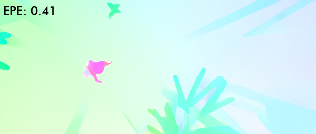
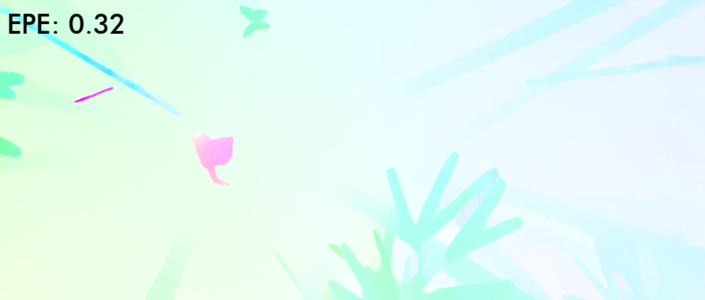
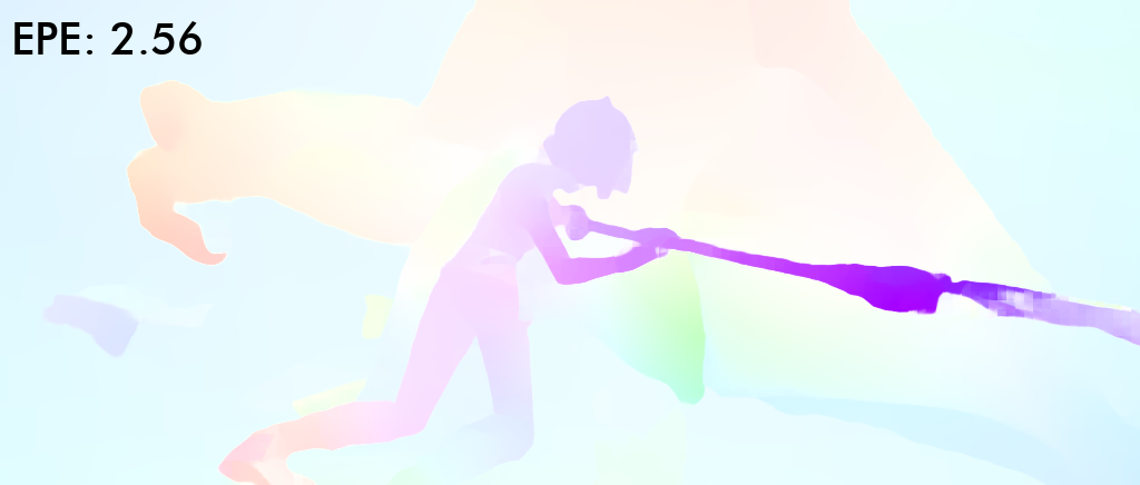
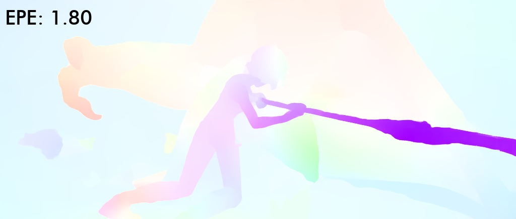
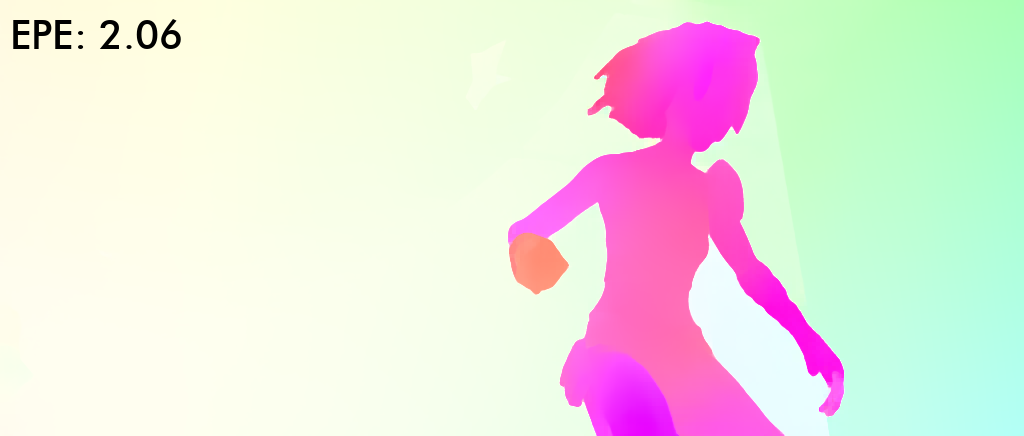
The improvements on Sintel clean can be attributed to the larger correlation volume ($1/4$ resolution vs $1/8$ resolution). We provide qualitative results in Figure 5, which clearly demonstrates the advantage of building the correlation volume and predicting optical flow in high resolutions. It can be seen that the motion of fine structures fails to be captured by RAFT but can be accurately predicted by our approach, with the use of a $1/4$ resolution correlation volume. With Sintel final and KITTI-15, there exists significantly more motion blur and featureless regions. Therefore, setting $k=8$ might be too small to reach the same performance as a dense correlation volume. We analyse the effect of $k$ in Section 3.3 via ablation experiments. We want to emphasize that even though we do not outperform RAFT[29] in all datasets, it is surprising to see that a sparse approach can do almost as well given the few storage of correlation values. For each pixel, we store and process only $k=8$ correlations whereas RAFT requires to store $h\times w$ correlations, limiting its ability to scale up to higher resolutions.

	Method	Chairs (val)	Sintel (train)		KITTI-15 (train)
			Clean	Final	EPE	F1-all
Resolution	Eighth	0.95	1.55	3.07	5.74	20.2
	Quarter	0.71	1.29	2.95	6.80	19.3
Ours Sparsity⋆	$k=1$	1.14	1.97	3.44	7.56	25.6
	$k=4$	0.98	1.72	3.07	6.32	21.8
	$k=8$	0.95	1.55	3.07	5.74	20.2
RAFT Sparsity [29]	$k=1$	1.20	3.13	4.26	14.4	39.3
	$k=8$	0.93	1.64	2.97	7.18	22.8
	$k=32$	0.87	1.50	2.82	5.77	19.5
	$k=128$	0.84	1.50	2.75	5.61	19.0
	ReLU	0.91	1.44	2.75	5.09	16.7
	Dense	0.88	1.44	2.73	5.10	17.5

Table 2: Ablation experiment results. Settings used in our final model are underlined. The details are in Section 3.3. We also give results run on RAFT’s original code but with varying sparsity levels of the correlation volume. ^⋆We ran these experiments on $1/8$ resolution.

Sparsity	$1/4$ Resolution		$1/8$ Resolution
	Size	Memory	Size	Memory
Dense	$7.8\times 10^{8}$	$3.1\text{\,}\mathrm{GB}$	$4.8\times 10^{7}$	$191\text{\,}\mathrm{MB}$
$k=8$	$2.2\times 10^{5}$	$0.9\text{\,}\mathrm{MB}$	$5.5\times 10^{4}$	$0.2\text{\,}\mathrm{MB}$
$k=32$	$8.9\times 10^{5}$	$3.6\text{\,}\mathrm{MB}$	$2.2\times 10^{5}$	$0.9\text{\,}\mathrm{MB}$
$k=128$	$3.6\times 10^{6}$	$14.3\text{\,}\mathrm{MB}$	$8.8\times 10^{5}$	$3.5\text{\,}\mathrm{MB}$

(a) Size and memory of a correlation volume based on a pair of images of size $436\times 1024$. Size refers to the number of elements and the correlation volumes are stored in 32-bit floats.

Method	batch = 1	batch = 2
RAFT [29]	10.6 GB	20.0 GB
Ours	6.1 GB	9.3 GB

(b) Actual memory consumption when training on the Sintel dataset. The correlation volumes are built from $1/4$ resolution feature maps. We use a random crop of $400\times 720$. The batch size is set to $1$ and $2$.

Table 3: Results for memory consumption.

3.3 Ablation Study

We conducted ablation experiments to validate our hypothesis that top-$k$ correlations are sufficient to give a good representation of the full correlation volume. The main setting here is how large should $k$ be. We show results on our model with different choices of $k$ on $1/8$ resolutions. It can be clearly seen that larger $k$ gives better performance. Even when $k=1$, the results are still reasonable and do not completely fail.

We also compare $1/4$ resolution correlation volume with $1/8$ resolution correlation volume and we can see that $1/4$ resolution correlation volume gives better results in all datasets except the EPE in KITTI-15. Since large correlation volumes are constructed from higher-resolution feature maps, we believe that larger correlation volumes are more descriptive of the image details and the results agree with our hypothesis.

An additional experiment we conducted is with RAFT’s original implementation. We keep the top-$k$ elements in the correlation volume and set the rest to be zero. We vary $k$ to be $\{1,8,32,128\}$. In Table 2, ReLU refers to setting all negative values to be zero and only keeping the positive correlations. We also trained with the original code which is denoted as “Dense”. We can see that larger $k$ gives better results and $k=\{32,128\}$ almost reach the same performance as the dense method. ReLU even outperforms the dense method on KITT-15. This again validates our hypothesis that there exists significant redundancy in the current dense approach and a sparse correlation volume with a large enough $k$ could do just as well.

3.4 Memory Consumption

Our method of processing the sparse correlation volume does not introduce new learning parameters. The number of parameters in our network is $5.3\text{\,}\mathrm{MB}$, which is the same as RAFT. Given an image pair of size $436\times 1024$, the size and memory of sparse correlation volumes and dense correlation volumes in $1/4$ and $1/8$ resolutions are listed in Table 3(a).

When correlation volumes are built from $1/8$ resolution feature maps, our approach does not lead to a significant memory saving. This is due to the constant $2\text{\,}\mathrm{GB}$ memory overhead of the $k$NN search library and also the correlation volume is not a memory bottleneck ($191\text{\,}\mathrm{MB}$ when batch size = 1) when resolutions are small.

However, our approach demonstrates a clear advantage when correlation volumes are built from $1/4$ resolution feature maps for images of size $436\times 1024$. When training at $1/4$ resolution, with a random crop of $400\times 720$ of the original image and batch size = 1 and 2, our approach consumes around $50\%$ of total memory compared to RAFT. The results are demonstrated in Table 3(b). This showcases the effectiveness of our approach in saving memory when correlation volumes are scaled to higher resolutions.

3.5 Limitations

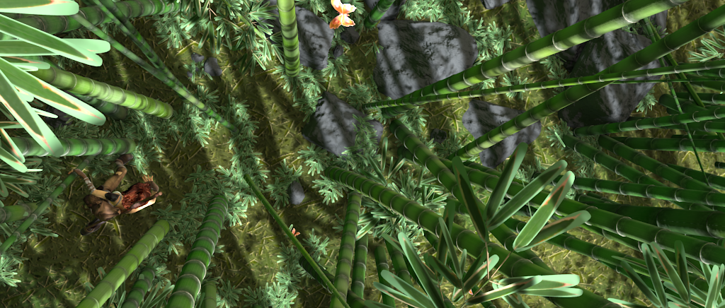
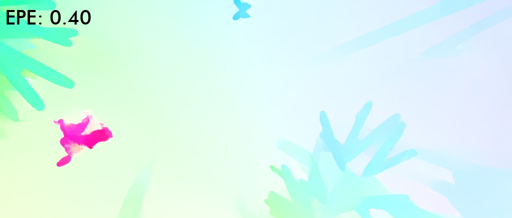
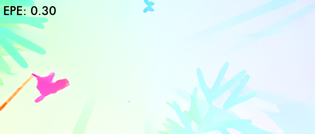
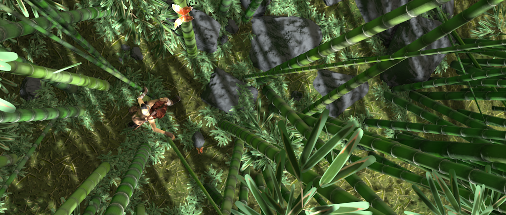
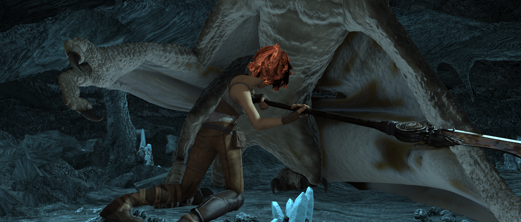
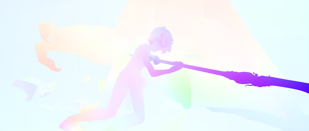
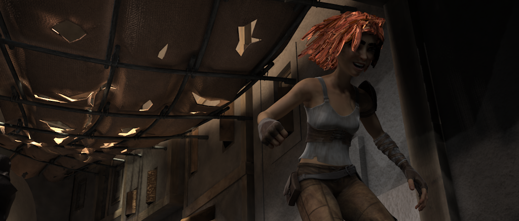
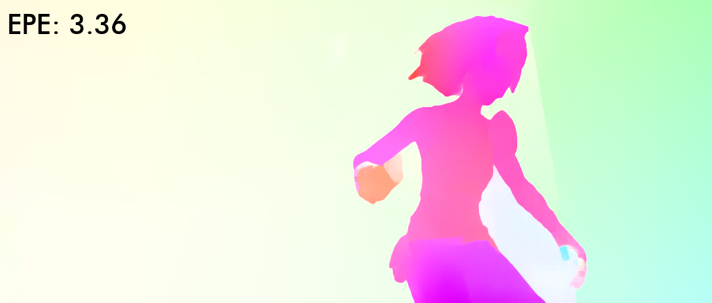
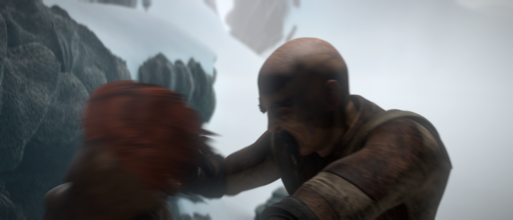
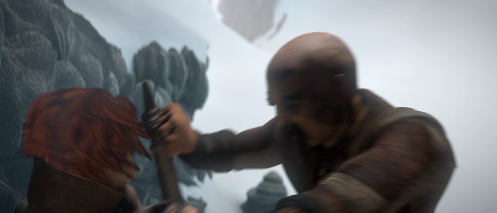
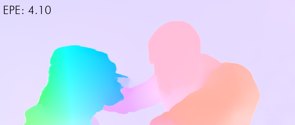
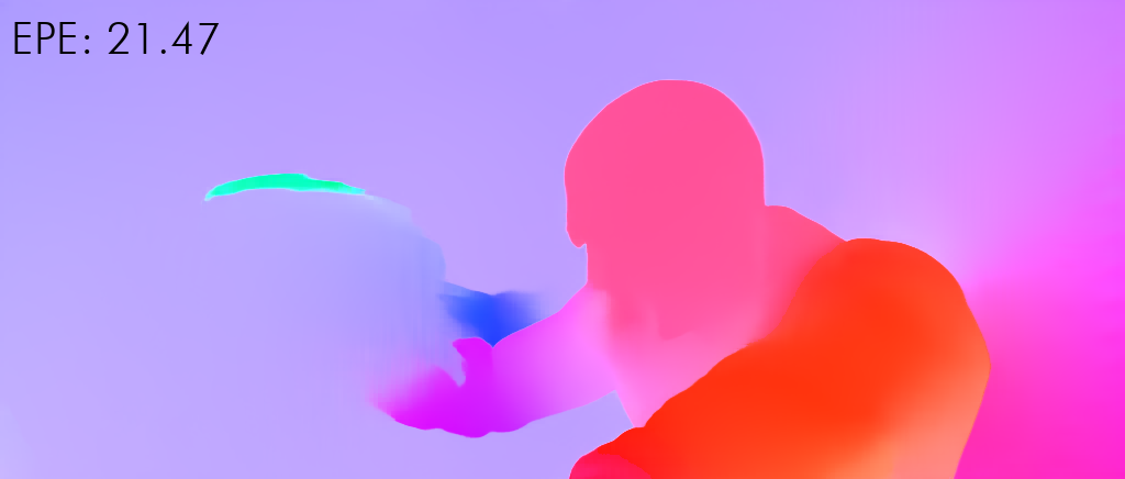
Increasing the resolution to $1/4$, we have observed consistent improvements on fine-structure motions (the bamboo sequence in Sintel). However, the commonly used metric for overall evaluation, mean EPE, is defined to be biased towards large motions on large regions. One particular weakness of our approach is the handling of featureless or blurry regions. Such features typically have a large number of matches due to the ambiguity, top-$k$ might not be sufficient to cover the correct match and could give misguided motion prediction. An example failure case is shown in Figure 6. One can see that the red hair contains significant motion blur, where our top-$k$ correlations do not contain the correct matches hence lead to incorrect prediction.

(a) Image 1

(b) Image 2

(c) GT

(d) RAFT

(e) Ours

Figure 6: An example failure case. When the scene contains significant featureless regions or motion blur, top-$k$ correlations may not contain the correct matches and can lead to incorrect flow prediction.

4 Related Work

Optical flow was first formulated as a continuous optimization problem with variational approaches [11]. Various subsequent papers have worked on on improving robustness [2] and energy term [35], incorporating descriptor matching into energy minimization [4] and improving regularizations [26]. Accurate flow fields can be predicted when displacements are small. However, their performances are limited at large displacements, due to the use of first order Taylor approximation.

Pyramidal approaches were developed to handle large displacements in stereo and optical flow, pioneered by Quam et al.[25]. Traditional methods build a Gaussian pyramid [5] and predict optical flow or stereo in a coarse-to-fine manner. In contrast, deep optical flow approaches [27, 34, 13, 14, 15, 33, 1, 36, 30] build a feature pyramid to extract more representative information on different levels through learning. Optical flows are then predicted in a coarse-to-fine manner. A local correlation volume with a limited search range is constructed in each level, based on featured maps warped with the upsampled flow from the previous level. This approach limits the search range of the correlation volume and effectively reduces the memory and computational cost for processing it. However, as pointed out in previous works [20, 10, 29], pyramidal warping approaches can have ghosting effects at occlusions. They are also limited at handling the small object large motion problem and fine-level predictions often fail to recover errors made in coarser levels. By contrast, our method operates at a single resolution and does not suffer from such problems.

Pyramidal approaches are designed to handle large motions while keeping memory cost small. However, they are not the only successful approach to dealing with large motions. Before the deep learning era, optical flow estimation was formulated as a discrete optimization problem by solving a Markov random field (MRF) [3]. Chen et al.[7] proposed a one-shot global discrete optimization approach at a single resolution with a distance transform, which is then refined using continuous optimization. Menze et al.[22] proposed reducing the search space by limiting to a fixed number $k$ matches per pixel via approximate nearest neighbour search. Our idea is similar in the sense that we both limit the search space to top-$k$, but rather than solving an MRF, we propose explicitly constructing a sparse correlation volume and using iterative refinement to predict optical flow. The main difference is that our final solution does not necessarily lie the top-$k$ solution space, which gives better occlusion handling. Our idea is also inspired by the recent paper on learning to find sparse matches, which proposed to find top-$k$ matches first then process with sparse convolutions. However, we do not use sparse convolutions but rather convert the sparse correlation volume to a dense tensor with our proposed multi-scale displacement encoder.

A recent breakthrough in deep optical flow estimation has been achieved by RAFT [29], which proposed constructing a dense all-pairs correlation volume on a single resolution and adopting a recurrent network to iteratively predict optical flow. Due to the memory cost of the correlation volume, the feature map resolutions are limit to $1/8$ of the original image resolution. Our approach is different to RAFT in three major ways:

1. Rather than constructing a dense all-pairs correlation volume, we construct a sparse correlation volume where only the top $k$ correlations are stored. This allows us to reduce the spatial complexity from $O(N^{2})$ to $O(N)$, where $N$ refers to the number of pixels of an image.

2. Because of the savings in memory cost, we can build the correlation volume from higher resolution feature maps ($1/4$ vs. $1/8$) without limiting the searching range. This allows our method to accurately predict the motion of the finer structures.

3. We propose a new way of iteratively decoding the sparse correlation volume. Rather than sampling in a dense correlation volume at different locations, we iteratively update the coordinates of the sparse correlation volume and apply “bilinear splatting” to splat the correlations onto the integer grids.

5 Conclusions

Since the publication of RAFT [29], the use of all-pairs (large displacements) correlation volume is becoming a standard way of solving for optical flow due to its superior performance compared to pyramidal approaches. However, the memory consumption of an all-pairs correlation volume grows quadratically with the number of pixels, quickly limiting its ability to handle high-resolution images or capture fine-structure motion. We observed a rather surprising fact where storing just the top-$k$ correlations provides almost as good results as storing the dense correlation volume. The sparse correlation volume method proposed in this paper provides an alternative approach to store the all-pairs matching information which massively reduces memory consumption while gives accurate prediction of optical flow. Experiments validated the feasibility of using sparse correlation volume in optical flow estimation tasks. We believe our paper has paved a way for future optical flow research directions, where the memory requirement of correlation volumes is no longer a limiting factor.

References

- [1] Aviram Bar-Haim and Lior Wolf. Scopeflow: Dynamic scene scoping for optical flow. CVPR, 2020.
- [2] Michael J Black and Padmanabhan Anandan. A framework for the robust estimation of optical flow. ICCV, 1993.
- [3] Yuri Boykov and Vladimir Kolmogorov. An experimental comparison of min-cut/max-flow algorithms for energy minimization in vision. TPAMI, 2004.
- [4] Thomas Brox, Christoph Bregler, and Jitendra Malik. Large displacement optical flow. CVPR, 2009.
- [5] Peter Burt and Edward Adelson. The laplacian pyramid as a compact image code. IEEE Transactions on communications, 1983.
- [6] D. J. Butler, J. Wulff, G. B. Stanley, and M. J. Black. A naturalistic open source movie for optical flow evaluation. ECCV, 2012.
- [7] Qifeng Chen and Vladlen Koltun. Full flow: Optical flow estimation by global optimization over regular grids. CVPR, 2016.
- [8] Christopher Choy, JunYoung Gwak, and Silvio Savarese. 4d spatio-temporal convnets: Minkowski convolutional neural networks. CVPR, 2019.
- [9] Alexey Dosovitskiy, Philipp Fischer, Eddy Ilg, Philip Hausser, Caner Hazirbas, Vladimir Golkov, Patrick Van Der Smagt, Daniel Cremers, and Thomas Brox. Flownet: Learning optical flow with convolutional networks. ICCV, 2015.
- [10] Markus Hofinger, Samuel Rota Bulò, Lorenzo Porzi, Arno Knapitsch, Thomas Pock, and Peter Kontschieder. Improving optical flow on a pyramid level. ECCV, 2020.
- [11] Berthold KP Horn and Brian G Schunck. Determining optical flow. Techniques and Applications of Image Understanding, 1981.
- [12] Asmaa Hosni, Christoph Rhemann, Michael Bleyer, Carsten Rother, and Margrit Gelautz. Fast cost-volume filtering for visual correspondence and beyond. TPAMI, 2012.
- [13] Tak-Wai Hui, Xiaoou Tang, and Chen Change Loy. Liteflownet: A lightweight convolutional neural network for optical flow estimation. CVPR, 2018.
- [14] Tak-Wai Hui, Xiaoou Tang, and Chen Change Loy. A lightweight optical flow cnn-revisiting data fidelity and regularization. TPAMI, 2020.
- [15] Junhwa Hur and Stefan Roth. Iterative residual refinement for joint optical flow and occlusion estimation. CVPR, 2019.
- [16] Eddy Ilg, Nikolaus Mayer, Tonmoy Saikia, Margret Keuper, Alexey Dosovitskiy, and Thomas Brox. Flownet 2.0: Evolution of optical flow estimation with deep networks. CVPR, 2017.
- [17] Jeff Johnson, Matthijs Douze, and Hervé Jégou. Billion-scale similarity search with gpus. arXiv preprint arXiv:1702.08734, 2017.
- [18] Alex Kendall, Hayk Martirosyan, Saumitro Dasgupta, Peter Henry, Ryan Kennedy, Abraham Bachrach, and Adam Bry. End-to-end learning of geometry and context for deep stereo regression. ICCV, 2017.
- [19] Daniel Kondermann, Rahul Nair, Katrin Honauer, Karsten Krispin, Jonas Andrulis, Alexander Brock, Burkhard Gussefeld, Mohsen Rahimimoghaddam, Sabine Hofmann, Claus Brenner, et al. The hci benchmark suite: Stereo and flow ground truth with uncertainties for urban autonomous driving. CVPR Workshop, 2016.
- [20] Yao Lu, Jack Valmadre, Heng Wang, Juho Kannala, Mehrtash Harandi, and Philip Torr. Devon: Deformable volume network for learning optical flow. WACV, 2020.
- [21] N. Mayer, E. Ilg, P. Häusser, P. Fischer, D. Cremers, A. Dosovitskiy, and T. Brox. A large dataset to train convolutional networks for disparity, optical flow, and scene flow estimation. CVPR, 2016.
- [22] Moritz Menze, Christian Heipke, and Andreas Geiger. Discrete optimization for optical flow. GCPR, 2015.
- [23] Moritz Menze, Christian Heipke, and Andreas Geiger. Joint 3d estimation of vehicles and scene flow. ISPRS Workshop on Image Sequence Analysis (ISA), 2015.
- [24] Adam Paszke, Sam Gross, Soumith Chintala, Gregory Chanan, Edward Yang, Zachary DeVito, Zeming Lin, Alban Desmaison, Luca Antiga, and Adam Lerer. Automatic differentiation in pytorch. NIPS Workshop, 2017.
- [25] Lynn H Quam. Hierarchical warp stereo. Readings in Computer Vision, 1987.
- [26] René Ranftl, Kristian Bredies, and Thomas Pock. Non-local total generalized variation for optical flow estimation. ECCV, 2014.
- [27] Deqing Sun, Xiaodong Yang, Ming-Yu Liu, and Jan Kautz. Pwc-net: Cnns for optical flow using pyramid, warping, and cost volume. CVPR, 2018.
- [28] Deqing Sun, Xiaodong Yang, Ming-Yu Liu, and Jan Kautz. Models matter, so does training: An empirical study of cnns for optical flow estimation. TPAMI, 2019.
- [29] Zachary Teed and Jia Deng. Raft: Recurrent all-pairs field transforms for optical flow. ECCV, 2020.
- [30] Jianyuan Wang, Yiran Zhong, Yuchao Dai, Kaihao Zhang, Pan Ji, and Hongdong Li. Displacement-invariant matching cost learning for accurate optical flow estimation. NeurIPS, 2020.
- [31] Jia Xu, René Ranftl, and Vladlen Koltun. Accurate optical flow via direct cost volume processing. CVPR, 2017.
- [32] Li Xu, Jiaya Jia, and Yasuyuki Matsushita. Motion detail preserving optical flow estimation. TPAMI, 2011.
- [33] Gengshan Yang and Deva Ramanan. Volumetric correspondence networks for optical flow. NeurIPS, 2019.
- [34] Zhichao Yin, Trevor Darrell, and Fisher Yu. Hierarchical discrete distribution decomposition for match density estimation. CVPR, 2019.
- [35] Christopher Zach, Thomas Pock, and Horst Bischof. A duality based approach for realtime tv-l 1 optical flow. Joint Pattern Recognition Symposium, 2007.
- [36] Shengyu Zhao, Yilun Sheng, Yue Dong, Eric I Chang, Yan Xu, et al. Maskflownet: Asymmetric feature matching with learnable occlusion mask. CVPR, 2020.