Efficient Magnus-type integrators for solar energy conversion in Hubbard models

Abstract

Strongly interacting electrons in solids are generically described by Hubbard-type models, and the impact of solar light can be modeled by an additional time-dependence. This yields a finite dimensional system of ordinary differential equations (ODE)s of Schrödinger type, which can be solved numerically by exponential time integrators of Magnus type. The efficiency may be enhanced by combining these with operator splittings. We will discuss several different approaches of employing exponential-based methods in conjunction with an adaptive Lanczos method for the evaluation of matrix exponentials and compare their accuracy and efficiency. For each integrator, we use defect-based local error estimators to enable adaptive time-stepping. This serves to reliably control the approximation error and reduce the computational effort.

url]http://www.asc.tuwien.ac.at/ winfried/ url]https://www.ifp.tuwien.ac.at/cms/ url]http://harald-hofstaetter.at url]https://www.ifp.tuwien.ac.at/cms/ url]http://www.othmar-koch.org url]https://mat.ug.edu.pl/ kmalina/ url]https://www.pranavsingh.co.uk/ url]https://www.ifp.tuwien.ac.at/cms/

1 Introduction

The time evolution of a quantum mechanical system is generally described by a system of linear ordinary differential equations (ODE)’s of Schrödinger type

$$\psi^{\prime}(t)=-\mathrm{i}H(t)\psi(t)=:A(t)\psi(t),\qquad\psi(t_{0})=\psi_{0},$$ (1.1)

with a large time-dependent Hermitian system matrix $H(t)$, state vector $\psi(t)$ at time $t$, and its derivative $\psi^{\prime}(t)$. The exact flow of (1.1) is denoted by $\psi(t)=\mathcal{E}(t;t_{0})\psi_{0},$ and depends on the initial state $\psi_{0}$ and time $t_{0}$. We will focus on the movement and interaction of electrons within Hubbard-type models, with the time dependence originating from electric fields associated with a photon in the process of solar energy conversion [1, 2]. These models naturally have a discrete, and for a finite number of lattice sites finite, basis set in which the matrix $H(t)$ can be expressed.

The present study is motivated by a recent application where the efficient time propagation of models of the type (1.1) is of paramount importance: The simulation of oxide solar cells with the goal of finding candidates for new materials promising a gain in the solar cells’ efficiency [3, 1, 4]. For traditional materials such as silicon the efficiency of solar cells is fundamentally limited to 34% due to the Schockley–Queisser limit [5]. For overcoming this limit and building highly efficient solar cells, [3] recently proposed a (for this purpose new) class of materials: oxide heterostructures. These consist of at least two different transition metal oxides. One of these can be the cheap and commonly used substrate material, the perovskite SrTiO₃. On top of this, one can stack layers of, e.g., LaVO₃ which has a preferable bandgap of $\sim 1.1\,$eV for photovoltaic applications. The equilibrium calculations of [3] have indicated the great potential of these oxide heterostructures for solar cells; and a LaVO₃/SrTiO₃ solar cell was experimentally realized in [6], and likewise a LaFeO₃/SrTiO₃ one [7]. A particular advantage of these oxide heterostructure solar cells is that one photon may excite two electron-hole pairs through a secondary process called impact ionization [8, 1, 4]. This might serve to overcome the Schockley–Queisser limit. However, for actually improving the efficiency of these solar cells, a better understanding and calculation of the nonequilibrium processes, which are at the heart of the solar energy conversion, are direly needed. Indeed, so far the efficiency of the solar cell has not been calculated as this results from an inherently nonequilibrium process.

In this paper, we compare numerical time integrators for the efficient approximation of the full dynamics of solar energy conversion in Hubbard models on a finite number of lattice sites. The methods which are commonly considered as most appropriate for this task are based on the matrix exponential function. When the latter is suitably approximated, the time propagation conserves the norm of the wave function, which is the case for the Lanczos method we employ, see Section 3.5. This is violated, however, for popular one-step methods such as Runge–Kutta, which is used for the purpose of comparisons in this study only. Our emphasis is on adaptive time-stepping based on asymptotically correct estimates of the local error. The advantage of adaptive step-size choice lies not only in the potential for increased efficiency when the smoothness of the solution varies over time, but more importantly in the reliable control of the accuracy. The computational effort for the evaluation of the error estimate may not always be compensated for by the optimal choice of the local step-size. However, an optimal equidistant step-size cannot usually be guessed a priori, while adaptive step-size selection automatically adapts the time-steps such that the prescribed error tolerance is satisfied. Hence, the accuracy of the numerical approximation is reliably controlled.

The methods which we focus on are commutator-free Magnus-type methods [9, 10], but also classical Magnus integrators are considered [11, 12]. Furthermore, a Magnus-Lanczos integrator employing operator splitting, inspired by [13], is tested. Explicit Runge–Kutta methods are used for the purpose of comparisons.

In Section 2 we describe the simple model of solar energy conversion in oxide solar cells which we investigate. Section 3 describes the numerical methods which we consider, and Section 4 gives the results of our comparative tests. A provides a detailed description of the construction and implementation of a new splitting-based Magnus–Strang integrator designed especially for problems of the structure we are confronted with. Finally, B presents some supplementary numerical tests.

2 The model

For the description of the Hubbard model we resort to the second-quantization formalism. The Hubbard model first appears in [14, 15, 16] and since then became the basic model for describing strongly interacting (strongly correlated) electrons [17, 18]. It describes the electron occupation on a given number of sites, corresponding to Wannier discretization. Only a single orbital per site is considered which allows for four states per site (no electron, one electron with spin-up or -down, two electrons). If there are two electrons on the same site this costs a Coulomb interaction $U$. The Hubbard Hamiltonian for arbitrary hopping $v_{ij}$ reads

$$H=\frac{1}{2}\sum_{i,j,\sigma}v_{ij}\hat{c}_{j\sigma}^{\dagger}\hat{c}_{i\sigma}^{\phantom{\dagger}}+\frac{1}{2}\sum_{i,\sigma}U\hat{n}_{i\sigma}\hat{n}_{i\bar{\sigma}},$$ (2.1)

where $i,j$ sum over all $N$ sites and the spins $\sigma,\sigma^{\prime}\in\{\uparrow,\downarrow\}$ are either up or down, and $\bar{\sigma}$ is the spin opposite to $\sigma$. The notation $\hat{c}_{j\sigma}^{\dagger}c_{i\sigma}^{\phantom{\dagger}}$ describes a “hopping” from site $i$ to $j$ with creation and annihilation operators $\hat{c}_{j\sigma}^{\dagger}$ and $\hat{c}_{i\sigma}$, respectively. The hopping amplitudes $v_{ij}$ with $i,j=1,\ldots,N$ give the probability (rate) of such an electron hopping; $\hat{n}_{j\sigma}=\hat{c}_{j\sigma}^{\dagger}\hat{c}_{j\sigma}^{\phantom{\dagger}}$ is the occupation number operator, which counts the number of electrons with spin $\sigma$ at site $j$. A derived observable which we will use later is the mean double occupation $\langle\hat{d}(t)\rangle=\frac{1}{N}\sum_{i=1}^{N}\langle\psi(t)|\hat{d}_{i}|\psi(t)\rangle,$ where the expectation value of $\hat{d}_{i}=\hat{n}_{i\uparrow}\hat{n}_{i\downarrow}$ is 1 (0) if there are two (zero or one) electrons on site $i$. For details on the notation in (2.1) we recommend several references, e.g. [14, 17, 18, 19].

The time-dependence in the Hamiltonian (2.1) is introduced through the photon which excites the system out of equilibrium. We approximate the photon by a classical electric field pulse of the form $\vec{E}(t)=\vec{E}_{0}{\mathrm{e}}^{-(t-t_{p})^{2}/\sigma_{p}^{2}}\sin(\omega(t-t_{p}))$, where $\omega$ denotes the frequency (energy) of the photon, $\sigma_{p}$ the width in time and $t_{p}$ the point in time of its impact. We can relate $\vec{E}(t)=-\partial_{t}\vec{A}(t)$ to a vector potential $\vec{A}(t)$ using a gauge without scalar potential. The vector potential in turn can be related, within the Peierls’ approximation [20], to a modified hopping amplitude [21, 22, 1]

$$v_{ij}\rightarrow v_{ij}(t)=v_{ij}{\mathrm{e}}^{\mathrm{i}\int_{{\mathbf{R}}_{i}}^{{\mathbf{R}}_{j}}\vec{A}({\mathbf{r}^{\prime}},t)\,{\mathrm{d}}{\mathbf{r}^{\prime}}},$$ (2.2)

where ${\mathbf{R}}_{i}$ is the position of lattice site $i$.

For our numerical tests we use Hubbard models with different geometric settings.

1. First, we model $8$ electrons on $8$ sites ($N=8$) arranged in a two-dimensional $2\times 4$ ladder with open boundary conditions, with spin up and down for each site. A graphical illustration of the geometry is given in Figure 1. Such an electron distribution is also referred to as half-filled in the literature. We furthermore restrict our model by considering the number of electrons with spin up or down to be fixed as $N/2$, respectively. This leads to $n=\genfrac{(}{)}{0.0pt}{1}{8}{4}^{2}=4900$ considered occupation states which create a discrete basis. Without restriction on the number of electrons and their spin, we would have $4^{N}=65536$ states. For the numerical implementation of the basis we consider $16$-bit integers for which each bit describes a position which is occupied in case the bit is equal to $1$ or empty otherwise. The set of occupation states can be ordered by the value of the integers which leads to a unique representation of the Hubbard Hamiltonian (2.1) by a matrix $H\in\mathbb{C}^{n\times n}$. Such an implementation of the Hubbard Hamiltonian is also described in [2] and [19, Section 3].

2. Secondly, we use a $4\times 3$ lattice ($N=12$). The state is again assumed as half-filled, that is, $12$ electrons populate the $12$ sites (6 with each spin). This leads to $n=\genfrac{(}{)}{0.0pt}{1}{12}{6}^{2}=853776$ occupation states. The basis is also encoded by $16$-bit integers, analogously as in the $2\times 4$ case. [2].

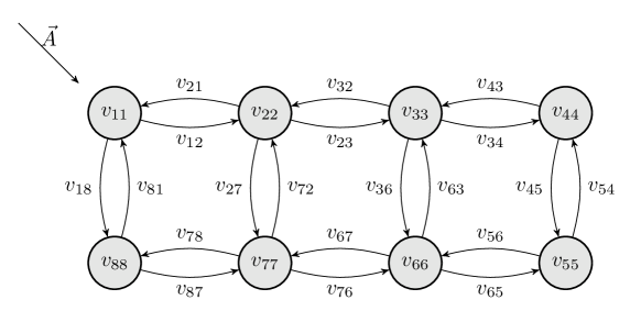
Figure 1: Geometry of a two-dimensional $8$-site lattice ($2\times 4$ ladder) with lexicographical ordering of the sites. The energies $v_{ii}$ describe the on-site potential, $v_{ij}$ describe the hoppings between sites $i$ and $j$. The vector potential $\vec{A}$ of the electromagnetic field is in the lattice plane and in the diagonal direction.

In our first test setting, the $2\times 4$ ladder, we use $U=4$ and a local potential $v_{11}=v_{88}=v_{44}=v_{55}=-1.75$ and $v_{22}=v_{33}=v_{66}=v_{77}=-2.25$ (see Fig.1). Hopping is only allowed between nearest neighbors (with open boundary conditions). The absolute value of the nonzero $v_{i,j\neq i}$ elements is constant and equal to $1$. This sets our energy units, whereas the unit of time $t$ is the inverse of the energy unit (which corresponds to setting $\hbar\equiv 1$).

For this choice of $v_{ij}$ we obtain an Hermitian matrix $H(t)\in\mathbb{C}^{n\times n}$ with $60864$ nonzero entries for the $2\times 4$ ladder geometry. The spectrum of $H(t)$ is independent of $t$ and the eigenvalues lie within the interval $(-21.04,5.23)$. This is because the electric field (2.2) only modifies the phase of the nearest neighbor hopping elements according to

$$v_{ij}(t)=v_{ij}\underbrace{\exp\left({\mathrm{i}}a(\cos(\omega(t-t_{p}))-b)\,{\mathrm{e}}^{-\frac{(t-t_{p})^{2}}{2\sigma_{p}^{2}}}\right)}_{=:f(t)},$$ (2.3)

whereas the local terms $v_{ii}$ are constant in time. Mathematically speaking, the described Hamiltonian $H_{\rm full}(t)$ is isospectral, since it satisfies [23, Def. 8.3.8, Property A]. This also implies that in a Lanczos algorithm for the approximation of the matrix exponential, the size of the subspace can be fixed for all $t$. For our tests we choose $t_{p}=6$, $a=0.2$, $\sigma_{p}=2$, $\omega=3.5$, and $b=\cos(\omega t_{p})$ for the $2\times 4$ ladder. In supplementary comparisons given in B we also vary the parameters in the $2\times 4$ geometry and choose $\sigma_{p}=1,\ 4$ and $\omega=1.75,\ 7$ to corroborate our findings on the efficiency of the adaptive methods.

For the $4\times 3$ geometry, we use $U=8$, $v_{ii}=-4$ (the same for all sites), and the hopping elements $v_{ij}$ are again nonzero only for nearest neighbor sites $i$ and $j$ and given by (2.3) (which corresponds to a diagonal in-plane field). The parameters are as follows: $t_{p}=7.5$, $\sigma_{p}=2$, $a=0.8$, $\omega=11$, and $b=\cos(\omega t_{p})$. In the $4\times 3$ case we have $16687440$ nonzero entries of $H(t)$ and its eigenvalues lie within the interval $(-52.92,4.92)$. For this set of parameters, impact ionization has been found [24].

Separating a constant diagonal contribution, which includes $v_{ii}$ and $U$, and splitting of the off-diagonal contribution into real and imaginary part, this model leads to a Hamiltonian of the structure

$$H_{\rm full}(t)=H_{\rm diag}+\underbrace{{\rm Re}(f(t))}_{=:\,c(t)}H_{\rm symm}+{\mathrm{i}}\underbrace{{\rm Im}(f(t))}_{=:\,s(t)}H_{\rm anti}=H_{\rm full}^{\ast}(t),$$ (2.4)

with real matrices $H_{\rm diag}$, $H_{\rm symm}$, and $H_{\rm anti}$, where $H_{\rm diag}$ is diagonal, $H_{\rm symm}$ is symmetric, and $H_{\rm anti}$ is skew-symmetric. Note that the time-dependence is only present in the scalar function $f(t)$, while the matrices are constant. This structure will be exploited in a new time integrator using operator splitting, which we introduce in Section 3.4, see also A.

3 Numerical approaches

We consider Magnus-type one-step methods for the approximation of (1.1) on a time grid $(t_{0},t_{1},\dots,t_{n},\dots)$,

$$\psi_{n+1}={\mathcal{S}}(\tau_{n};t_{n})\,\psi_{n}\approx\psi(t_{n+1})=\mathcal{E}(\tau_{n};t_{n})\,\psi(t_{n}),\quad\tau_{n}=t_{n+1}-t_{n}\,,\quad n=0,1,2,\ldots\,,$$

where $\mathcal{E}(\tau_{n};t_{n})$ denotes the exact and ${\mathcal{S}}(\tau_{n};t_{n})$ the approximated unitary operator for the time propagation from $t_{n}$ to $t_{n}+\tau_{n}$. For the description of the schemes, in the following we use a simplified notation for a single step starting from $t=t_{0}$ with stepsize $\tau$,

$$\psi_{1}={\mathcal{S}}(\tau;t_{0})\,\psi_{0}\approx\psi(t_{0}+\tau)\,.$$ (3.1)

In order to avoid unnecessary overloading of notation, we suppress the dependence on $t_{0}$ of ‘internal’ objects involved in the definition of the integrators. Only the dependence on the stepsize $\tau$ is indicated; see for instance (3.2) below.

In the following, we will put our emphasis on approximations of order four, as this is usually sufficient for the accuracy required, and the splitting-based integrator described in Section 3.4 has this order. All the exponential-based time integrators considered in this study are symmetric (time-reversible), which is a desirable property when the reversible flow of a Schrödinger-type equation is approximated.

3.1 Commutator-free Magnus-type (CFM) integrators

A successful and much used class of integration methods is comprised of higher-order commutator-free Magnus-type integrators [9, 25]. These approximate the exact flow in terms of products of exponentials of linear combinations of the system matrix evaluated at different times, avoiding evaluation and storage of commutators.

A high-order CFM scheme starting at $t=t_{0}$ is thus defined by (3.1), with the ansatz [9, 25]

$${\mathcal{S}}(\tau;t_{0}) ={\mathcal{S}}_{J}(\tau)\cdots{\mathcal{S}}_{1}(\tau)={\mathrm{e}}^{\Omega_{J}(\tau)}\,\cdots\,{\mathrm{e}}^{\Omega_{1}(\tau)}\,,$$ (3.2)

$$\Omega_{j}(\tau) =\tau B_{j}(\tau),~{}~{}j=1,\ldots,J,$$

$$B_{j}(\tau) =\sum_{k=1}^{K}a_{jk}\,A_{k}(\tau),\qquad A_{k}(\tau)=A(t_{0}+c_{k}\tau)\,,$$

where the coefficients $a_{jk}$, $c_{k}$ are determined from the order conditions (a system of polynomial equations in the coefficients) such that the method realizes a certain convergence order $p$, see for example [26] and references therein. Algorithms to efficiently generate the order conditions are described for instance in [27]. The solution of this system of equations is generally not unique, and numerical optimization techniques are employed to compute solutions that are optimal in some sense, for instance minimizing in some sense the leading local error term of the ensuing integrator.

Examples of symmetric CFM integrators

1. The second-order scheme ($p=2$) given by

   $$J=1,\quad K=1,\qquad c=\tfrac{1}{2},\quad a=1\,,$$

   is a simple instance of a Magnus-type integrator, commonly denoted as exponential midpoint rule. It yields

   $${\mathcal{S}}(\tau;t_{0})={\mathrm{e}}^{\tau A(t_{0}+\frac{\tau}{2})}\,.$$ (3.3)

   Note that this represents both a classical Magnus integrator and a commutator-free Magnus-type method. In the numerical tests, this method is referred to as CF2.

2. A fourth-order commutator-free integrator ($p=4$) based on two Gaussian nodes and comprising two matrix exponentials is defined by $J=K=2$ and

   $$c=\begin{pmatrix}\tfrac{1}{2}-\tfrac{\sqrt{3}}{6}\\ \tfrac{1}{2}+\tfrac{\sqrt{3}}{6}\end{pmatrix},\quad a=\begin{pmatrix}\frac{1}{4}+\frac{\sqrt{3}}{6}&\frac{1}{4}-\frac{\sqrt{3}}{6}\\[3.0pt] \frac{1}{4}-\frac{\sqrt{3}}{6}&\frac{1}{4}+\frac{\sqrt{3}}{6}\end{pmatrix}.$$ (3.4)

   In the numerical tests, this method is referred to as CF4.

3. An optimized fourth-order scheme ($p=4$) from [9] satisfies $J=K=3$ and

   $$c=\begin{pmatrix}\frac{1}{2}-\frac{\sqrt{15}}{10}\\[6.0pt] \frac{1}{2}\\[3.0pt] \frac{1}{2}+\frac{\sqrt{15}}{10}\end{pmatrix},\quad a=\begin{pmatrix}\frac{37}{240}+\frac{10}{87}\frac{\sqrt{15}}{3}&-\frac{1}{30}&\frac{37}{240}-\frac{10}{87}\frac{\sqrt{15}}{3}\\[6.0pt] -\frac{11}{360}&~{}\;\frac{23}{45}&-\frac{11}{360}\\[3.0pt] \frac{37}{240}-\frac{10}{87}\frac{\sqrt{15}}{3}&-\frac{1}{30}&\frac{37}{240}+\frac{10}{87}\frac{\sqrt{15}}{3}\end{pmatrix}.$$ (3.5)

   In the numerical tests, this method is referred to as CF4o.

4. Based on the approach for constructing new optimized commutator-free Magnus-type integrators described in [27, 28], we have constructed the following fourth-order numerical integrator with $J=K=3,$ but smaller leading error term:

   $$c=\begin{pmatrix}1/2-\sqrt{15}/10\\[6.0pt] 1/2\\[3.0pt] 2+\sqrt{15}/10\end{pmatrix},$$

   $$a_{11}=0.302146842308616954258187683416$$

   $$a_{12}=-0.030742768872036394116279742324$$

   $$a_{13}=0.004851603407498684079562131338$$

   $$a_{21}=-0.029220667938337860559972036973$$

   $$a_{22}=0.505929982188517232677003929089$$

   $$a_{23}=-0.029220667938337860559972036973$$

   $$a_{31}=0.004851603407498684079562131337$$

   $$a_{32}=-0.030742768872036394116279742324$$

   $$a_{33}=0.302146842308616954258187683417$$

   In the numerical tests, this method is referred to as CF4oH. Note that the coefficients have been determined numerically and are given to within double precision, likewise for the next schemes.

5. We have also constructed a new optimized method of order six with $K=3,\ J=4$:

   $$c=\begin{pmatrix}1/2-\sqrt{15}/10\\[6.0pt] 1/2\\[3.0pt] 1/2+\sqrt{15}/10\end{pmatrix},$$

   $$a_{11}=0.79124225942889763$$

   $$a_{12}=-0.080400755305553218$$

   $$a_{13}=0.01.2765293626634554$$

   $$a_{21}=-0.48931475164583259$$

   $$a_{22}=0.05.4170980027798808$$

   $$a_{23}=-0.012069823881924156$$

   $$a_{31}=-0.029025638294289255$$

   $$a_{32}=0.50138457552775674$$

   $$a_{33}=-0.02.5145341733509552$$

   $$a_{41}=0.0048759082890019896$$

   $$a_{42}=-0.030710355805557892$$

   $$a_{43}=0.30222764976657693$$

   In the numerical tests, this method is referred to as CF6n.

6. A new optimized method of order seven with $K=4,\ J=6$ is given by the coefficients

   $$c=\begin{pmatrix}-\sqrt{\tfrac{1}{140}(2\sqrt{30}+15)}+1/2\\[9.0pt] -\sqrt{\tfrac{1}{140}(-2\sqrt{30}+15)}+1/2\\[6.0pt] \sqrt{\tfrac{1}{140}(-2\sqrt{30}+15)}+1/2\\[3.0pt] \sqrt{\tfrac{1}{140}(2\sqrt{30}+15)}+1/2\end{pmatrix},$$

   $$a_{11}=0.205862188450411892209$$

   $$a_{12}=0.169508382914682544509$$

   $$a_{13}=-0.102088008415028059851$$

   $$a_{14}=0.0304554010755044437431$$

   $$a_{21}=-0.0574532495795307023280$$

   $$a_{22}=0.234286861311879288330$$

   $$a_{23}=0.332946059487076984706$$

   $$a_{24}=-0.0703703697036401378340$$

   $$a_{31}=-0.008.93040281749440468751$$

   $$a_{32}=0.02.71488489365780259156$$

   $$a_{33}=-0.02.95144169823456538040$$

   $$a_{34}=-0.151311830884601959206$$

   $$a_{41}=0.552299810755465569835$$

   $$a_{42}=-3.64425287556240176808$$

   $$a_{43}=2.53660580449381888484$$

   $$a_{44}=-0.661436528542997675116$$

   $$a_{51}=-0.538241659087501080427$$

   $$a_{52}=3.60578285850975236760$$

   $$a_{53}=-2.50685041783117850901$$

   $$a_{54}=0.651947409253201845106$$

   $$a_{61}=0.02.03907348473756540850$$

   $$a_{62}=-0.0664014986792173869631$$

   $$a_{63}=0.0949735566789294244299$$

   $$a_{64}=0.374643341371260411994$$

   In the numerical tests, this method is referred to as CF7.

Local error estimation

As a basis for adaptive time-stepping, defect-based error estimators for CFM methods and for classical Magnus integrators have been introduced in [29]. The (classical) defect is defined by

$${\mathcal{D}}(\tau)={\mathcal{S}}^{\prime}(\tau;t_{0})-A(t_{0}+\tau){\mathcal{S}}(\tau;t_{0})$$ (3.6)

and satisfies

$${\mathcal{D}}(0)={\mathcal{D}}^{\prime}(0)=\cdots={\mathcal{D}}^{(p-1)}(0)=0,$$

if the method coefficients $a,\ c$ satisfy the order conditions for an order $p$ method.

The local error ${\mathcal{L}}(\tau)\psi_{0}:=({\mathcal{S}}(\tau;t_{0})-\mathcal{E}(\tau;t_{0}))\psi_{0}$ can be expressed in terms of the defect via the variation-of-constant formula,

$${\mathcal{L}}(\tau)\psi_{0}=\int_{0}^{\tau}\Pi(\tau,\sigma){\mathcal{D}}(\sigma)\,{\mathrm{d}}\sigma={\mathscr{O}}(\tau^{p+1}),\quad\Pi(\tau,\sigma)=\mathcal{E}(\tau-\sigma;t_{0}+\sigma).$$

For the practical evaluation of the defect, the derivative of matrix exponentials of the form

$$\tfrac{{\mathrm{d}}}{{\mathrm{d}}\tau}{\mathrm{e}}^{\tau B(\tau)}=\Gamma(\tau)\,{\mathrm{e}}^{\tau B(\tau)}$$

is required. The function $\Gamma$ is given as an infinite series or alternatively as an integral expression, which are approximated by truncation or numerical Hermite quadrature, respectively, to yield a computable quantity $\tilde{\Gamma}$ and an approximate defect $\tilde{\mathcal{D}}$. The resulting computable error estimator is denoted by $\tilde{\mathcal{P}}$ in both cases. The asymptotical correctness of the error estimators was established in [29]. We recapitulate the result for the exponential midpoint rule (3.3):

Proposition: Consider the exponential midpoint rule (3.3).
If $A\in C^{3}$, then the local error ${\mathcal{L}}$ satisfies

$$\|{\mathcal{L}}(\tau)\|_{2}\leq\tfrac{1}{12}\tau^{3}\big{\|}[A(t_{0}),A^{\prime}(t_{0})]-\tfrac{1}{2}A^{\prime\prime}(t_{0})\|_{2}+{\mathscr{O}}(\tau^{4})\,.$$

If $A\in C^{4}$, then the deviation $\tilde{\mathcal{P}}(\tau)-{\mathcal{L}}(\tau)=\tfrac{1}{3}\tau\tilde{\mathcal{D}}(\tau)-{\mathcal{L}}(\tau)$ of the local error estimate satisfies

$$\|\tilde{\mathcal{P}}(\tau)-{\mathcal{L}}(\tau)\|_{2} \leq \tau^{4}\big{\|}c\,[A(t_{0}),[A(t_{0}),A^{\prime}(t_{0})]]-\tfrac{1}{48}[A(t_{0}),A^{\prime\prime}(t_{0})]$$ (3.7)

$$\qquad+\tfrac{1}{144}A^{\prime\prime\prime}(t_{0})\big{\|}_{2}+{\mathscr{O}}(\tau^{5})\,,$$

where $c=\tfrac{1}{72}$ for the approximate defect $\tilde{\mathcal{D}}(\tau)$, Taylor version, and $c=0$ for the approximate defect $\tilde{\mathcal{D}}(\tau)$, Hermite version.

In the numerical experiments reported in this paper, Hermite quadrature has been used throughout.

3.2 Classical Magnus integrators

A different, indeed the more classical, approach to the approximation of (1.1) is directly based on the Magnus expansion [12]: The solution to a time-dependent system (1.1) can be represented by

$$\psi(t_{0}+\tau)=\mathcal{E}(\tau;t_{0})\psi_{0}={\mathrm{e}}^{\bm{\Omega}(\tau)}\psi_{0}\,,$$ (3.8a)

where the matrix $$\bm{\Omega}(\tau)$$ satisfies

$$\bm{\Omega}^{\prime}(\tau)=\sum_{k\geq 0}\frac{{B_{k}}}{k!}\,\mathrm{ad}_{\bm{\Omega}(\tau)}^{k}(A(t_{0}+\tau))\,,\quad\bm{\Omega}(0)=0\,,$$ (3.8b)

with the Bernoulli numbers $B_{k}$ and $\mathrm{ad}_{\bm{\Omega}}^{k}(A)$ denoting the $k$-th iterated commutator of the matrices ${\bm{\Omega}}$ and $A$, see [11].

Classical Magnus integrators rely on appropriate truncation of the Magnus expansion (3.8b) and suitable approximation $\Omega(\tau)$ to the arising multi-dimensional integral representation for $\bm{\Omega}(\tau)$ by numerical quadrature, and defining $\psi_{1}$ by (3.1) with

$${\mathcal{S}}(\tau;t_{0})={\mathrm{e}}^{\Omega(\tau)}\approx{\mathrm{e}}^{\bm{\Omega}(\tau)}.$$ (3.9)

A detailed exposition on this approach is given for example in [30] and in [11], see also [31].

This type of integrator is, in general, considered as computationally expensive due to the requirement to compute and store commutators of large matrices. For problems of a particular structure, however, as in the semiclassical regime, where the small semiclassical parameter may render some of the appearing commutators negligibly small, or when commutators turn out to be of higher order $O(\tau^{k})$ than $O(1)$ as expected generically, this approach may excel over the commutator-free methods, see [9, 26, 32]. In our specially designed numerical integrator in Section 3.4 below, such a feature is actually exploited, see [13].

Examples of classical symmetric Magnus integrators

1. The exponential midpoint scheme (3.3) (order $p=2$) is also a classical Magnus integrator, with $K=1$ and

   $$c=\tfrac{1}{2}\,,\quad\Omega(\tau)=\tau A_{1}(\tau)\,.$$ (3.10)

2. A commonly used fourth-order Magnus integrator ($p=4$) is based on two Gaussian nodes, with $K=2$ and

   $$c=\begin{pmatrix}\tfrac{1}{2}-\tfrac{\sqrt{3}}{6}\\ \tfrac{1}{2}+\tfrac{\sqrt{3}}{6}\end{pmatrix},\quad\Omega(\tau)=\tfrac{1}{2}\tau\big{(}A_{1}(\tau)+A_{2}(\tau)\big{)}-\tfrac{\sqrt{3}}{12}\,\tau^{2}\big{[}A_{1}(\tau),A_{2}(\tau)\big{]}\,.$$ (3.11)

   In the numerical experiments, this is denoted as Magnus4.

Local error estimation

Classical Magnus integrators are of the form (3.9), where again $\Omega(\tau)=\tau B(\tau)$. Thus, the defect can be approximated analogously as in Section 3.1. Convergence of the integrators and asymptotical correctness of the error estimator has been proven in [29].

3.3 Symmetrized defect

When we consider self-adjoint (or symmetric) schemes which are characterized by the identity

$${\mathcal{S}}(-\tau;t_{0}+\tau)\,{\mathcal{S}}(\tau;t_{0})=\text{Id},$$ (3.12)

a higher asymptotical quality of the error estimator can be obtained at moderate additional expense by introducing a symmetrized version of the defect, which was introduced and analyzed in [33, 34]. We define

$${\mathcal{D}}_{{\bm{s}}}(\tau)={\mathcal{S}}^{\prime}(\tau;t_{0})-\tfrac{1}{2}\big{(}A(t_{0}+\tau){\mathcal{S}}(\tau;t_{0})+\partial_{2}{\mathcal{S}}(\tau;t_{0})+{\mathcal{S}}(\tau;t_{0})A(t_{0})\big{)},$$ (3.13)

where $\partial_{2}$ stands for differentiation with respect to the second argument. A local error representation based on a symmetrized variation-of-constant formula in conjunction with numerical quadrature again yields an asymptotically correct error estimator. Since the exponential-based integrators we used in this study are symmetric, the symmetric version of the error estimator has been used throughout.

Example: Exponential midpoint rule [34]

Let

$${\mathcal{R}}(\tau;t_{0})(\,\cdot\,)=\tfrac{{\mathrm{d}}}{{\mathrm{d}}\Omega}{\mathrm{e}}^{\Omega}\big{|}_{\Omega=\tau A(t_{0}+\frac{\tau}{2})}(\,\cdot\,),$$

where $\tfrac{{\mathrm{d}}}{{\mathrm{d}}\Omega}{\mathrm{e}}^{\Omega}$ denotes the Fréchet derivative of the matrix exponential, see (3.16) below. Then, for the exponential midpoint rule (3.3)

$${\mathcal{S}}^{\prime}(\tau;t_{0}) ={\mathcal{R}}(\tau;t_{0})\big{(}A(t_{0}+\tfrac{\tau}{2})+\tfrac{1}{2}\tau A^{\prime}(t_{0}+\tfrac{\tau}{2})\big{)},$$

$$\partial_{2}{\mathcal{S}}(\tau;t_{0}) ={\mathcal{R}}(\tau;t_{0})\big{(}\tau A^{\prime}(t_{0}+\tfrac{\tau}{2})\big{)}.$$

This gives the following defect representations:

• Classical defect (3.6):

  $${\mathcal{D}}_{{\bm{c}}}(\tau)={\mathcal{R}}(\tau;t_{0})\big{(}A(t_{0}+\tfrac{\tau}{2})+\tfrac{1}{2}\tau A^{\prime}(t_{0}+\tfrac{\tau}{2})\big{)}-A(t_{0}+\tau){\mathcal{S}}(\tau;t_{0}).$$ (3.14)

• Symmetrized defect (3.13):

  $${\mathcal{D}}_{{\bm{s}}}(\tau)={\mathcal{R}}(\tau;t_{0})\big{(}A(t_{0}+\tfrac{\tau}{2})\big{)}-\tfrac{1}{2}\big{(}A(t_{0}+\tau){\mathcal{S}}(\tau;t_{0})+{\mathcal{S}}(\tau;t_{0})A(t_{0})\big{)}.$$ (3.15)

Here, the explicit representation

$${\mathcal{R}}(\tau;t_{0})\big{(}V\big{)} =\int_{0}^{1}{\mathrm{e}}^{\sigma\tau A(t_{0}+\frac{\tau}{2})}V{\mathrm{e}}^{-\sigma\tau A(t_{0}+\frac{\tau}{2})}\,{\mathrm{d}}\sigma\cdot{\mathcal{S}}(\tau;t_{0})$$ (3.16)

follows from [35, (10.15)]. For evaluating (3.14), a sufficiently accurate quadrature approximation for the integral according to (3.16) is required. This involves evaluation of $A^{\prime}$ and the commutator $[A,A^{\prime}]$, see [34]. In contrast, the relevant term from (3.15) simplifies to

$${\mathcal{R}}(\tau;t_{0})\big{(}A(t_{0}+\tfrac{\tau}{2})\big{)} =A(t_{0}+\tfrac{\tau}{2}){\mathcal{S}}(\tau;t_{0})={\mathcal{S}}(\tau;t_{0})A(t_{0}+\tfrac{\tau}{2}),$$

whence the symmetrized defect (3.15) can be evaluated exactly,

$${\mathcal{D}}_{{\bm{s}}}(\tau) ={\mathcal{S}}(\tau;t_{0})\big{(}A(t_{0}+\tfrac{\tau}{2})-\tfrac{1}{2}A(t_{0})\big{)}-\tfrac{1}{2}A(t_{0}+\tau){\mathcal{S}}(\tau;t_{0}).$$ (3.17)

This involves an additional application of ${\mathcal{S}}(\tau;t_{0})$, but it does not require evaluation of the derivative $A^{\prime}$ or of a commutator expression. We also note that the applications of ${\mathcal{S}}$ from left and right can be evaluated in parallel.

The deviation of the symmetrized error estimator used in conjunction with the exponential midpoint rule as compared to the exact local error satisfies an estimate of the form

$$\|\tilde{\mathcal{P}}(\tau)-{\mathcal{L}}(\tau)\|_{2}={\mathscr{O}}(\tau^{5}),$$

see [34].

3.4 Fourth order Magnus-Strang splitting

Magnus expansion

To obtain a new efficient fourth-order method for problems of the structure (2.4), we proceed similarly as in [13]. We start using only the first two terms of the Magnus expansion (3.8) for the solution of (1.1),

$$\psi(t_{0}+\tau)={\rm e}^{\mathbf{\Omega}(\tau)}\psi_{0}\approx{\rm e}^{\Omega_{2}(\tau)}\psi_{0}+\mathcal{O}(\tau^{5}),$$

with

$$\begin{split}\Omega_{2}(\tau)&=\int_{t_{0}}^{t_{0}+\tau}-{\mathrm{i}}\,H_{\rm full}(\zeta)\,{\rm d}\zeta+\frac{1}{2}\int_{t_{0}}^{t_{0}+\tau}\int_{t_{0}}^{t_{0}+\zeta}[-{\mathrm{i}}\,H_{\rm full}(\zeta),-{\mathrm{i}}\,H_{\rm full}(\xi)]\,{\rm d}\xi\,{\rm d}\zeta\\ &=\underbrace{\Big{(}-{\mathrm{i}}\int_{t_{0}}^{t_{0}+\tau}H_{\rm full}(\zeta)\,{\rm d}\zeta\Big{)}}_{\mathcal{A}(\tau;t_{0})=\mathcal{O}(\tau)}+\underbrace{\Big{(}-\frac{1}{2}\int_{t_{0}}^{t_{0}+\tau}\int_{t_{0}}^{t_{0}+\zeta}[H_{\rm full}(\zeta),H_{\rm full}(\xi)]\,{\rm d}\xi\,{\rm d}\zeta\Big{)}}_{\mathcal{B}(\tau;t_{0})=\mathcal{O}(\tau^{3})},\end{split}$$ (3.18)

where $\mathcal{A}(\tau;t_{0})$ and $\mathcal{B}(\tau;t_{0})$ are again skew-Hermitian. Here, because the time-dependence in (2.4) is given by two scalars $s(t)$ and $c(t)$, $\mathcal{A}(\tau;t_{0})$ is simple to evaluate,

$$\int_{t_{0}}^{t_{0}+\tau}H_{\rm full}(\xi)\,{\rm d}\xi=tH_{\rm diag}+H_{\rm symm}\int_{t_{0}}^{t_{0}+\tau}c(\xi)\,{\rm d}\xi+{\mathrm{i}}H_{\rm anti}\int_{t_{0}}^{t_{0}+\tau}s(\xi)\,{\rm d}\xi,$$

while evaluation of $\mathcal{B}(\tau;t_{0})$ at first sight seems more challenging. It involves evaluation of the commutator

$$[H_{\rm full}(\zeta),H_{\rm full}(\xi)] =c(\xi)[H_{\rm diag},H_{\rm symm}]+{\mathrm{i}}\,s(\xi)[H_{\rm diag},H_{\rm anti}]$$

$$\quad{}+c(\zeta)[H_{\rm symm},H_{\rm diag}]+{\mathrm{i}}\,s(\zeta)[H_{\rm anti},H_{\rm diag}]$$

$$\quad{}+{\mathrm{i}}\,c(\zeta)s(\xi)[H_{\rm symm},H_{\rm anti}]+{\mathrm{i}}\,c(\xi)s(\zeta)[H_{\rm anti},H_{\rm symm}]$$

$$=\left(c(\zeta)-c(\xi)\right)[H_{\rm symm},H_{\rm diag}]+{\mathrm{i}}\left(s(\zeta)-s(\xi)\right)[H_{\rm anti},H_{\rm diag}]$$

$$\quad{}+{\mathrm{i}}\left(c(\zeta)s(\xi)-c(\xi)s(\zeta)\right)[H_{\rm symm},H_{\rm anti}].$$ (3.19)

Since $H_{\rm diag}$, $H_{\rm symm}$, and $H_{\rm anti}$ do not depend on time, the computation of $\int_{t_{0}}^{t_{0}+\tau}\int_{t_{0}}^{t_{0}+\zeta}[H_{\rm full}(\zeta),H_{\rm full}(\xi)]\,{\rm d}\xi\,{\rm d}\zeta$ boils down to the evaluation of the following integrals, which can be simplified as indicated:

$$\begin{split}&\int_{t_{0}}^{\tau}\int_{t_{0}}^{t_{0}+\zeta}\big{(}c(\zeta)-c(\xi)\big{)}\,{\rm d}\xi\,{\rm d}\zeta=2\int_{t_{0}}^{t_{0}+\tau}c(\zeta)\big{(}\zeta-\tfrac{\tau}{2}\big{)}\,{\rm d}\zeta,\\ &\int_{t_{0}}^{t_{0}+\tau}\int_{t_{0}}^{t_{0}+\zeta}\big{(}s(\zeta)-s(\xi)\big{)}\,{\rm d}\xi\,{\rm d}\zeta=2\int_{t_{0}}^{t_{0}+\tau}s(\zeta)(\zeta-\tfrac{\tau}{2})\,{\rm d}\zeta,\\ &\int_{t_{0}}^{t_{0}+\tau}\int_{t_{0}}^{t_{0}+\zeta}\big{(}c(\zeta)s(\xi)-c(\xi)s(\zeta)\big{)}\,{\rm d}\xi\,{\rm d}\zeta\\ &\quad=\int_{t_{0}}^{t_{0}+\tau}c(\zeta)\,{\rm d}\zeta\int_{t_{0}}^{t_{0}+\tau}s(\xi)\,{\rm d}\xi-2\int_{t_{0}}^{t_{0}+\tau}c(\zeta)\int_{t_{0}+\zeta}^{t_{0}+\tau}s(\xi)\,{\rm d}\xi\,{\rm d}\zeta.\end{split}$$ (3.20)

The splitting

To obtain a practical fourth order method we proceed in a similar way as indicated in [13]. Applying Strang splitting to (3.18) yields

$${\rm e}^{\frac{1}{2}\mathcal{A}(\tau;t_{0})}{\rm e}^{\mathcal{B}(\tau;t_{0})}{\rm e}^{\frac{1}{2}\mathcal{A}(\tau;0)}={\rm e}^{\mathbf{\Omega}(\tau;t_{0})}+\mathcal{O}(\tau^{5}),$$

or alternatively

$${\rm e}^{\frac{1}{2}\mathcal{B}(\tau;t_{0})}{\rm e}^{\mathcal{A}(\tau;t_{0})}{\rm e}^{\frac{1}{2}\mathcal{B}(\tau;t_{0})}={\rm e}^{\mathbf{\Omega}(\tau)}+\mathcal{O}(\tau^{5}).$$

Which of the two splitting variants is favorable depends on the properties of the operators $\mathcal{A}$ and $\mathcal{B}$. For the present problem the splitting can be realized in an efficient way, expressing $\mathcal{A}$ and $\mathcal{B}$ in the form

$$\mathcal{A}(\tau;t_{0}) =-{\mathrm{i}}\,\big{(}\tau H_{\rm diag}+\tilde{c}_{1}(\tau,t_{0})H_{\rm symm}+{\mathrm{i}}\,\tilde{s}_{1}(\tau,t_{0})H_{\rm anti}\big{)}$$

$$=-{\mathrm{i}}\,\tau H_{\rm diag}-{\mathrm{i}}\,\tilde{c}_{1}(\tau,t_{0})H_{\rm symm}+\tilde{s}_{1}(\tau,t_{0})H_{\rm anti},$$

and (see (3.19))

$$\mathcal{B}(\tau;t_{0})=-\tilde{c}_{2}(\tau,t_{0})[H_{\rm symm},H_{\rm diag}]-{\mathrm{i}}\,\tilde{s}_{2}(\tau,t_{0})[H_{\rm anti},H_{\rm diag}]-{\mathrm{i}}\,\tilde{r}(\tau,t_{0})[H_{\rm symm},H_{\rm anti}],$$

where (see (3.20))

$$\tilde{c}_{1}(\tau;t_{0}) =\int_{t_{0}}^{t_{0}+\tau}c(\zeta)\,{\rm d}\zeta=\mathcal{O}(\tau),\quad\tilde{s}_{1}(\tau;t_{0})=\int_{t_{0}}^{t_{0}+\tau}s(\zeta)\,{\rm d}\zeta=\mathcal{O}(\tau),$$

$$\tilde{c}_{2}(\tau;t_{0}) =\int_{t_{0}}^{t_{0}+\tau}c(\zeta)(\zeta-\tfrac{\tau}{2})\,{\rm d}\zeta=\mathcal{O}(\tau^{3}),$$

$$\tilde{s}_{2}(\tau;t_{0}) =\int_{t_{0}}^{t_{0}+\tau}s(\zeta)(\zeta-\tfrac{t}{2})\,{\rm d}\zeta=\mathcal{O}(\tau^{3}),$$

$$\tilde{r}(\tau;t_{0}) =\tfrac{1}{2}\int_{t_{0}}^{t_{0}+\tau}c(\zeta)\,{\rm d}\zeta\int_{t_{0}}^{t_{0}+\tau}s(\xi)\,{\rm d}\xi-\int_{t_{0}}^{t_{0}+\tau}c(\zeta)\int_{t_{0}+\zeta}^{t_{0}+\tau}s(\xi)\,{\rm d}\xi\,{\rm d}\zeta=\mathcal{O}(\tau^{3}),$$

and apply Strang splitting as before. Implementation details for this integrator are explained in A. In the numerical experiments, this method is denoted as MagnusStrang4.

Remark 1

Methods based on a Strang splitting of the Magnus expansion were found to be very effective when the integrand is highly oscillatory [13, 36]. Note that due to the special scalings of $\mathcal{A}$ and $\mathcal{B}$, this splitting is actually of order four [13].

3.5 Adaptive Lanczos method

In each step of any of the introduced Magnus-type methods, the action of a matrix exponential

$$E(t)v={\mathrm{e}}^{-{\mathrm{i}}t\Omega}v,\quad\text{$\Omega$\ Hermitian},$$ (3.21)

has to be approximated. The standard Krylov approximation is

$$S_{m}(t)v=V_{m}\,{\mathrm{e}}^{-{\mathrm{i}}tT_{m}}\,V_{m}^{\ast}\,v=V_{m}\,{\mathrm{e}}^{-{\mathrm{i}}tT_{m}}e_{1},$$ (3.22)

with $T_{m}=(\tau_{i,j})$ tridiagonal and $V_{m}$ an orthonormal basis of the Krylov space $\mathcal{K}_{m}(\Omega,v)=\mathrm{span}\{v,\Omega v,\ldots,\Omega^{m-1}v\}\subseteq\mathbb{C}^{n}$. For Hermitian or skew-Hermitian matrices $\Omega$, this can be realized cheaply by the Lanczos method [37]. In [38], a time-stepping strategy was introduced which is based on the defect of the approximation. Due to the success of this strategy documented ibidem, we use it invariantly throughout our numerical experiments. The asymptotically correct error estimator is described in the following:

First, we define the defect operator

$$D_{m}(t)=-{\mathrm{i}}\,\Omega\,S_{m}(t)-S_{m}^{\prime}(t)\in\mathbb{C}^{n\times n}.$$

Then the local error operator $L_{m}(t)=E(t)-S_{m}(t)$ enjoys the representation

$$L_{m}(t)v=\int_{0}^{t}E(t-s)\,D_{m}(s)v\,{\mathrm{d}}s.$$

This defect-based integral representation yields a computable, asymptotically correct local error bound ($\gamma_{m}=\prod_{j=1}^{m-1}(T_{m})_{j+1,j})$, satisfying (see [38]).

$$\|L_{m}(t)v\|_{2}\leq\tau_{m+1,m}\gamma_{m}\,\frac{t^{m}}{m!},$$

$$\|L_{m}(t)v\|_{2}=\tau_{m+1,m}\gamma_{m}\,\frac{t^{m}}{m!}+{\mathcal{O}}(t^{m+1}).$$

4 Numerical experiments

In this section, we give the results of our numerical experiments to assess the accuracy, reliability and efficiency of the numerical time integrators investigated in this work. In all the experiments, the tolerance for the adaptive Lanczos method for the matrix exponential was set to $10^{-12}$. This limits the accuracy that can be obtained by the time integrators, which manifests itself as an apparent order reduction for the smallest time-steps in some cases. Supplementary tests given in B show similar results.

First we study the $2\times 4$ ladder geometry in Figures 2 and 3, second a $4\times 3$ lattice in Figures 4 and 5.

Figures 2 and 4 show in the left plots the error of the computation as a function of equidistant time-steps. The step-sizes are consecutively halved such that $\tau=2^{-k},\ k=0,\dots,5$. The error here is computed relative to a reference solution which was obtained with a tolerance $10^{-11}$. We observe that the theoretical convergence orders are well reflected in the empirically determined orders from the numerical experiments. Note the apparent order reduction for the highest precisions, which is to be attributed to the limited accuracy of the reference solution.

The right plots in Figures 2 and 4 show the error as a function of matrix-vector multiplications in the computation of the matrix exponentials. In fact, most of the computational effort arising in the context of exponential integrators is associated with this source. Observe that indeed, the plots show a systematic convergence order similarly as the error/$dt$ plots. The results are, however, also influenced by the fact that the Lanczos method requires more iterations when the time-step is larger, see for example [39, 40, 41, 42].

Generally, the highest-order methods CF7 and CF6n have the highest accuracy, where the benefits of the order 7 approximation are still superimposed by a larger error constant and CF6n fares better in terms of the number of matrix-vector multiplications. The advantages of the high-order methods are manifest especially for high accuracies. A comparison of the fourth-order methods show that CF4o and CF4oH are almost indistinguishable for the $2\times 4$ geometry, but the latter is slightly more accurate for the $4\times 3$ model in Fig.4. Both the classical Magnus4 integrator and the new MagnusStrang4 method suffer from large error constants. The envisaged advantage manifests itself in the accuracy as compared to the number of matrix-vector multiplications, however. The new integrator thus shows its advantage over the classical Magnus integrator, as was proposed in [13]. Particularly it reduces the effort for the Lanczos process, but the optimized commutator-free methods are clearly advantageous, especially in their high-order variants. The second order exponential midpoint rule is not competitive.

In this study, we put an emphasis on the adaptive implementation of the time-stepping methods. Thus, we compare the achieved accuracy with the number of matrix-vector multiplications in the respective left-hand plots in Figures 3 and 5. We observe that apparently, the error estimators for the high-order methods are expensive to compute, and the fourth order methods are most efficient if adaptive time-stepping is included. For the reason of comparisons, we have also tested adaptive Runge–Kutta methods which are very popular as they are easy to implement and use, and state-of-the-art-implementations are widely available. However, for the problem class under consideration, both the Dormand/Prince method [43] (DoPri45 in the graphics) and an improved method by Tsitouras [44] Tsit45 fail significantly to achieve the prescribed tolerance, and are thus the least reliable, and also inefficient integrators.

For this comparison of the usefulness of adaptive strategies, reliability is also an important criterion. In the right-hand side plots in Figures 3 and 5, we thus show the quotients of the achieved accuracy over the prescribed accuracy (as a function of the number of matrix multiplications). Values significantly larger than 1 indicate a very unreliable adaptive strategy which fails to reach the prescribed tolerance, while values smaller than 1 signify an inefficient procedure which induces more computational effort than is actually required to reach the tolerance. We observe that for most exponential-based methods, this quotient is slightly smaller than 1, where the highest-order methods are the most unreliable, but the adaptive Runge–Kutta methods fail by far to satisfy the tolerance criterion. The non-optimized commutator-free Magnus-type integrators CF4 and (to a lesser degree) CF2 fall below the prescribed tolerance requirement most noticeably.

From the experiments, we can rule out explicit Runge–Kutta methods as appropriate integrators for the problem class we consider. The picture is similar for both the tested models.

Figures 2–5 also allow an assessment of the computational advantage of adaptive time-stepping over equidistant grids. If we compare equal levels on the $y$-axis in Figures 2 (right plot) and 3 (left plot), for the $2\times 4$ geometry, and likewise Figures 4 (right plot) and 5 (left plot) for the $4\times 3$ geometry for the same integrators, we observe that the same error level can be obtained at a smaller computational effort in the adaptive computations for the majority of time integrators. Additional tests, performed for different choices of the parameters $\sigma_{p}$ and $\omega$ are given in B. These confirm the picture inferred here.

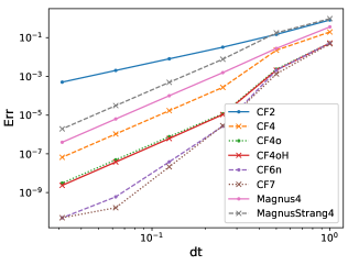
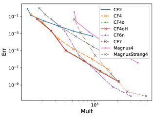
Figure 2: $2\times 4$ geometry, equidistant time-steps. Error as a function of the step-size (left) and as a function of matrix-vector multiplications (right).

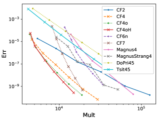
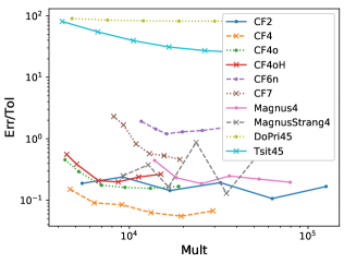
Figure 3: $2\times 4$ geometry, adaptive time-stepping. Error as a function of matrix-vector multiplications (left) and quotient $\frac{\mathrm{error}}{\mathrm{tolerance}}$ (right).

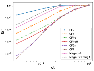
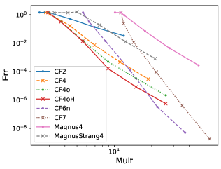
Figure 4: $4\times 3$ geometry, equidistant time-steps. Error as a function of the step-size (left) and as a function of matrix-vector multiplications (right).

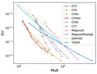
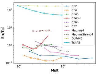
Figure 5: $4\times 3$ geometry, adaptive time-stepping. Error as a function of matrix-vector multiplications (left) and quotient $\frac{\mathrm{error}}{\mathrm{tolerance}}$ (right).

Finally, we illustrate the appropriateness of our step-size selection strategy in the sense that the step-sizes are chosen according to the local smoothness of the solution. We use the $2\times 4$ ladder geometry in this experiment.

Figure 6 shows the stepsizes chosen in the course of the time integration. The local step-sizes stepsizes are shown as a function of time $t$ for the representative choice of methods DoPri45, CF4, CF4oH, and Magnus4. We observe that the Runge–Kutta method chooses by far the smallest time-steps, the optimized commutator-free Magnus-type method CF4oH allows the largest time-steps and the classical Magnus integrator Magnus4 and CF4 are comparable, with time-steps in between the other two methods.

Figure 7 shows the approximation quality of the two functionals energy and double occupation by the commutator-free Magnus-type method CF4oH. These quantities describe the energy transfer into the system and the number of electron-hole pairs (or double/single occupied sites) excited by the solar light, respectively. For both the reference solution computed by DoPri45 and for CF4oH a tolerance of $10^{-11}$ was imposed. The Runge–Kutta method chooses vanishingly small time-steps, thus the numerical solution is plotted as a solid line, and the dots along these curves represent the points chosen by the adaptive CF4oH method. We observe that at the beginning of the time propagation the time-steps are chosen as quite small, after attenuation of the external pulse, however, time-steps increase impressively, while still the approximation quality of the double occupation functional is remarkable: The approximations computed with the large time-steps chosen for CF4oH lie on the curve provided by the reference method, however not following the oscillations in between the solution points. Overall, 244 points are needed for CF4oH, while DoPri45 requires 26015 steps.

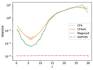
Figure 6: $2\times 4$ geometry. Adaptively chosen step-sizes for several integrators.

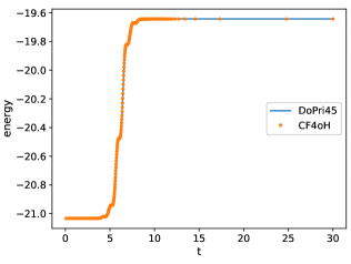
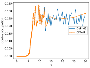
Figure 7: $2\times 4$ geometry. Approximation of the energy functional (left) and the mean double occupation functional (right) by optimized fourth-order commutator free Magnus integrators (CF4oH) and RRunge-Kutta (DoPri45).

5 Conclusions

In this study, we have investigated the successful application of adaptive Magnus-type exponential integrator for Hubbard models with a time-dependent electric field, modeling e.g. the impact of a solar photon. Similar Hamiltonians and time-dependencies will also be found in other situations where strongly interacting electrons are driven out-of-equilibrium by an external field. For such problems, commutator-free Magnus-type methods were found to be preferable over methods directly based on the Magnus expansion.

It was found that all methods show their expected convergence orders on coherent equidistant grids. However, the methods based on the Magnus expansion have larger error constants, where a newly proposed integrator improves on the classical fourth order Magnus integrator, but commutator-free methods are clearly to be favored. The use of high-order methods grants high accuracy for a given computational effort, especially when very precise solutions are sought.

We have also tested adaptive strategies based on asymptotically correct estimators of the local time-stepping error. Fourth order methods were found to be the most recommendable choice, where a new optimized method first presented in this work performs best. The popular and easy to implement explicit Runge–Kutta methods are not suitable for our problem class.

In addition to efficiency, reliability is a major motivation to use adaptive time-stepping strategies. Our tests revealed that commutator-free Magnus-type methods excel in that the prescribed tolerance and the actually achieved error are close (with high-order methods underestimating the necessary step-length more pronouncedly), while the classical Magnus integrator is too pessimistic (thus choosing unnecessarily small time-steps). Explicit Runge–Kutta methods are prohibitively unreliable.

Adaptive commutator-free Magnus-type methods are thus concluded to be the best choice for a reliable and efficient time integrators of Hubbard models of solar cells, with the best results for optimized fourth-order methods. This is also manifested by observing that important functionals of the solution like energy and mean double occupation are very well approximated even for large time-steps.

Appendix A Implementation details for the fourth order Magnus-Strang splitting

In this section, we give details of an efficient implementation of the new integrator proposed in Section 3.4 and the associated defect-based error estimator.

A.1 Basic integrator

For an effective numerical scheme we have to approximate the integrals in the definitions of $\mathcal{A}(\tau;t_{0})$ and $\mathcal{B}(\tau;t_{0})$. We obtain

$${\mathcal{S}}(\tau;t_{0})={\rm e}^{\frac{1}{2}\tau^{2}\Phi_{\mathcal{B}}(\tau;t_{0})}{\rm e}^{\tau\Phi_{\mathcal{A}}(\tau;t_{0})}{\rm e}^{\frac{1}{2}\tau^{2}\Phi_{\mathcal{B}}(\tau;t_{0})},$$ (A.1)

where

$$\Phi_{\mathcal{A}}(\tau;t_{0}) =-{\mathrm{i}}\,H_{\rm diag}-{\mathrm{i}}\,\hat{c}_{1}(\tau;t_{0})H_{\rm symm}+\hat{s}_{1}(\tau;t_{0})H_{\rm anti},$$

$$\Phi_{\mathcal{B}}(\tau;t_{0}) =-\hat{c}_{2}(\tau;t_{0})[H_{\rm symm},H_{\rm diag}]-{\mathrm{i}}\,\hat{s}_{2}(\tau,t_{0})[H_{\rm anti},H_{\rm diag}]-{\mathrm{i}}\,\hat{r}(\tau;t_{0})[H_{\rm symm},H_{\rm anti}]$$

with

$$\begin{split}\hat{c}_{1}(\tau;t_{0})&=\sum_{k=1}^{K_{1}}w^{(1)}_{k}c(t_{0}+x^{(1)}_{k}\tau)\approx\frac{1}{\tau}\tilde{c}_{1}(\tau,t_{0})=\frac{1}{\tau}\int_{t_{0}}^{t_{0}+\tau}c(\zeta)\,{\rm d}\zeta,\\ \hat{s}_{1}(\tau;t_{0})&=\sum_{k=1}^{K_{1}}w^{(1)}_{k}c(t_{0}+x^{(1)}_{k}\tau)\approx\frac{1}{\tau}\tilde{s}_{1}(\tau,t_{0})=\frac{1}{\tau}\int_{t_{0}}^{t_{0}+\tau}s(\zeta)\,{\rm d}\zeta,\\ \hat{c}_{2}(\tau;t_{0})&=\frac{1}{2}\sum_{k=1}^{K_{2}}w^{(2)}_{k}\big{(}c(t_{0}+y^{(2)}_{k}\tau)-c(t_{0}+x_{k}^{(2)}\tau)\big{)}\\ &\approx\frac{1}{\tau^{2}}\tilde{c}_{2}(\tau,t_{0})=\frac{1}{2\tau^{2}}\int_{t_{0}}^{t_{0}+\tau}\int_{t_{0}}^{t_{0}+\zeta}\big{(}c(\zeta)-c(\xi)\big{)}\,{\rm d}\xi\,{\rm d}\zeta,\\ \hat{s}_{2}(\tau;t_{0})&=\frac{1}{2}\sum_{k=1}^{K_{2}}w^{(2)}_{k}\big{(}s(t_{0}+y^{(2)}_{k}\tau)-s(t_{0}+x_{k}^{(2)}\tau)\big{)}\\ &\approx\frac{1}{\tau^{2}}\tilde{s}_{2}(\tau,t_{0})=\frac{1}{2\tau^{2}}\int_{t_{0}}^{\tau}\int_{t_{0}}^{t_{0}+\zeta}\big{(}s(\zeta)-s(\xi)\big{)}\,{\rm d}\xi\,{\rm d}\zeta,\\ \hat{r}(\tau;t_{0})&=\frac{1}{2}\sum_{k=1}^{K_{2}}w^{(2)}_{k}\big{(}c(t_{0}+y^{(2)}_{k}\tau)s(t_{0}+x^{(2)}_{k}\tau)-c(t_{0}+x_{k}^{(2)}\tau)s(t_{0}+y^{(2)}_{k}\tau)\big{)}\\ &\approx\frac{1}{\tau^{2}}\tilde{r}(\tau,t_{0})=\frac{1}{2\tau^{2}}\int_{t_{0}}^{t_{0}+\tau}\int_{t_{0}}^{t_{0}+\zeta}\big{(}c(\zeta)s(\xi)-c(\xi)s(\zeta)\big{)}\,{\rm d}\xi\,{\rm d}\zeta,\\ \end{split}$$

where $x^{(1)}_{k}$, $w^{(1)}_{k}$ respectively $x^{(2)}_{k}$, $y^{(2)}_{k}$, $w^{(2)}_{k}$ are the nodes and weights of a suitable quadrature formula for integration over the interval $[0,1]$ and over the triangle $0\leq y\leq 1$, $0\leq x\leq y$, respectively, see Tables 1, 2.

$x_{k}^{(1)}$	$w_{k}^{(1)}$
$\frac{1}{2}-\sqrt{\frac{1}{12}}$	$\frac{1}{2}$
$\frac{1}{2}+\sqrt{\frac{1}{12}}$	$\frac{1}{2}$

Table 1: Quadrature coefficients of order 4 for the interval $[0,1]$.

$x_{k}^{(2)}$	$y_{k}^{(2)}$	$w_{k}^{(2)}$
0.445948490915965	0.554051509084035	0.111690794839006
0.445948490915965	0.891896981831930	0.111690794839006
0.108103018168070	0.554051509084035	0.111690794839006
0.091576213509771	0.908423786490229	0.054975871827661
0.091576213509771	0.183152427019541	0.054975871827661
0.816847572980459	0.908423786490229	0.054975871827661

Table 2: Quadrature coefficients of order 4 for the triangle $0\leq y\leq 1$, $0\leq x\leq y$.

Note that for later convenience (for the definition of a defect-based error estimator) we extracted factors $\tau$ and $\tau^{2}$ in the exponents in (A.1).

The computation of the matrix–vector product

$$y=\Phi_{\mathcal{B}}(\tau;t_{0})\cdot v$$ (A.2)

is accomplished using the algorithm in Table 3.

$h_{1}=H_{\rm diag}\cdot v$ $h_{2}=H_{\rm symm}\cdot v$ $h_{3}=H_{\rm anti}\cdot v$ $h_{4}=-{\mathrm{i}}\hat{c}_{2}h_{1}+\hat{r}h_{3}$ $y=H_{\rm symm}\cdot h_{4}$ $h_{4}=\hat{s}_{2}h_{1}-\hat{r}h_{2}$ $h_{1}=H_{\rm anti}\cdot h_{4}$ $y=y+h_{1}$ $h_{4}=-{\mathrm{i}}\hat{c}_{2}h_{2}+\hat{s}_{2}h_{3}$ $h_{1}=H_{\rm diag}\cdot h_{4}$ $y=-{\mathrm{i}}(y-h_{1})$

Table 3: Algorithm for computing the matrix–vector product $y=\Phi_{\mathcal{B}}(\tau;t_{0})\cdot v$.

In addition to cheap scaling, addition, and subtraction operations on vectors this algorithm incorporates two (cheap) multiplications of vectors with $H_{\rm diag}$ and two multiplications of vectors each with $H_{\rm symm}$ and $H_{\rm anti}$. It needs four vectors $h_{1},\dots,h_{4}$ for the storage of intermediate results.

A.2 Implementation details for the symmetrized defect-based error estimator

The symmetrized defect here has the form

$${\mathcal{D}}(\tau)=(\partial_{\tau}-\tfrac{1}{2}\partial_{t_{0}}){\mathcal{S}}(\tau;t_{0})+\tfrac{1}{2}{\mathrm{i}}\big{(}H_{\rm full}(t_{0}+\tau){\mathcal{S}}(\tau;t_{0})+{\mathcal{S}}(\tau;t_{0})H_{\rm full}(t_{0})\big{)},$$

where $\partial_{\tau}$ denotes the derivative with respect to the first argument $\tau$, and $\partial_{t_{0}}$ denotes the derivative with respect to the second argument $t_{0}$. Here,

$$\begin{split}(\partial_{\tau}-\tfrac{1}{2}\partial_{t_{0}}){\mathcal{S}}(\tau;t_{0})=&\Gamma_{\mathcal{B}}(\tau;t_{0}){\rm e}^{\frac{1}{2}\tau^{2}\Phi_{\mathcal{B}}(\tau;t_{0})}{\rm e}^{\tau\Phi_{\mathcal{A}}(\tau,t_{0})}{\rm e}^{\frac{1}{2}\tau^{2}\Phi_{\mathcal{B}}(\tau;t_{0})}\\ &+{\rm e}^{\frac{1}{2}\tau^{2}\Phi_{\mathcal{B}}(\tau;t_{0})}\Gamma_{\mathcal{A}}(\tau;t_{0}){\rm e}^{\tau\Phi_{\mathcal{A}}(\tau;t_{0})}{\rm e}^{\frac{1}{2}\tau^{2}\Phi_{\mathcal{B}}(\tau;t_{0})}\\ &+{\rm e}^{\frac{1}{2}\tau^{2}\Phi_{\mathcal{B}}(\tau;t_{0})}{\rm e}^{\tau\Phi_{\mathcal{A}}(\tau;t_{0})}\Gamma_{\mathcal{B}}(\tau;t_{0}){\rm e}^{\frac{1}{2}\tau^{2}\Phi_{\mathcal{B}}(\tau;t_{0})}\end{split}$$

with

$$\Gamma_{\mathcal{A}}(\tau) =\int_{0}^{1}{\rm e}^{\sigma\tau\Phi_{\mathcal{A}}(\tau;t_{0})}(\partial_{\tau}-\tfrac{1}{2}\partial_{t_{0}})\big{(}\tau\Phi_{\mathcal{A}}(\tau;t_{0})\big{)}{\rm e}^{-\sigma\tau\Phi_{\mathcal{A}}(\tau;t_{0})}\,{\rm d}\sigma$$

$$=\Phi_{\mathcal{A}}(\tau;t)+\tau\int_{0}^{1}{\rm e}^{\sigma\tau\Phi_{\mathcal{A}}(\tau;t_{0})}\check{\Phi}_{\mathcal{A}}(\tau;t_{0}){\rm e}^{-\sigma\tau\Phi_{\mathcal{A}}(\tau;t_{0})}\,{\rm d}\sigma,$$ (A.3)

where

$$\check{\Phi}_{\mathcal{A}}(\tau;t_{0}) =(\partial_{1}-\tfrac{1}{2}\partial_{2})\Phi_{\mathcal{A}}(\tau;t_{0})=-{\mathrm{i}}\,\check{c}_{1}(\tau;t_{0})H_{\rm symm}+\check{s}_{1}(\tau;t_{0})H_{\rm anti},$$

$$\check{c}_{1}(\tau;t_{0}) =\sum_{k=1}^{K_{1}}w^{(1)}_{k}(x_{k}^{(1)}-\tfrac{1}{2})c^{\prime}(t_{0}+x^{(1)}_{k}\tau),$$

$$\check{s}_{1}(\tau;t_{0}) =\sum_{k=1}^{K_{1}}w^{(1)}_{k}(x_{k}^{(1)}-\tfrac{1}{2})s^{\prime}(t_{0}+x^{(1)}_{k}\tau),$$

and similarly,

$$\Gamma_{\mathcal{B}}(\tau;t_{0}) =\int_{0}^{1}{\rm e}^{\sigma\frac{1}{2}\tau^{2}\Phi_{\mathcal{B}}(\tau;t_{0})}(\partial_{\tau}-\tfrac{1}{2}\partial_{t_{0}})\big{(}\tfrac{1}{2}\tau^{2}\Phi_{\mathcal{B}}(\tau;t_{0})\big{)}{\rm e}^{-\sigma\frac{1}{2}\tau^{2}\Phi_{\mathcal{B}}(\tau;t_{0})}\,{\rm d}\sigma$$

$$=\tau\Phi_{\mathcal{B}}(\tau;t_{0})+\frac{\tau^{2}}{2}\int_{0}^{1}{\rm e}^{\sigma\frac{1}{2}\tau^{2}\Phi_{\mathcal{B}}(\tau;t_{0})}\check{\Phi}_{\mathcal{B}}(\tau;t_{0}){\rm e}^{-\sigma\frac{1}{2}\tau^{2}\Phi_{\mathcal{B}}(\tau;t_{0})}\,{\rm d}\sigma$$ (A.4)

with

$$\check{\Phi}_{\mathcal{B}}(\tau;t_{0})=-\check{c}_{2}(\tau;t_{0})[H_{\rm symm},H_{\rm diag}]-{\mathrm{i}}\,\check{s}_{2}(\tau,t_{0})[H_{\rm anti},H_{\rm diag}]-{\mathrm{i}}\,\check{r}(\tau,t_{0})[H_{\rm symm},H_{\rm anti}],$$

where

$$\check{c}_{2}(\tau;t_{0}) =\frac{1}{2}\sum_{k=1}^{K_{2}}w^{(2)}_{k}\big{(}(y_{k}^{(2)}-\tfrac{1}{2})c^{\prime}(t_{0}+y^{(2)}_{k}\tau)-(x_{k}^{(2)}-\tfrac{1}{2})c^{\prime}(t_{0}+x_{k}^{(2)}\tau)\big{)},$$

$$\check{s}_{2}(\tau,t_{0}) =\frac{1}{2}\sum_{k=1}^{K_{2}}w^{(2)}_{k}\big{(}(y_{k}^{(2)}-\tfrac{1}{2})s^{\prime}(t_{0}+y^{(2)}_{k}\tau)-(x_{k}^{(2)}-\tfrac{1}{2})s^{\prime}(t_{0}+x_{k}^{(2)}\tau)\big{)},$$

$$\check{r}(\tau,t_{0}) =\frac{1}{2}\sum_{k=1}^{K_{2}}w^{(2)}_{k}\big{(}(y_{k}^{(2)}-\tfrac{1}{2})c^{\prime}(t_{0}+y^{(2)}_{k}\tau)s(t_{0}+y^{(2)}_{k}\tau)+(x_{k}^{(2)}-\tfrac{1}{2})c(t_{0}+y^{(2)}_{k}\tau)s^{\prime}(t_{0}+y^{(2)}_{k}\tau)$$

$$\qquad\qquad\ \ -(x_{k}^{(2)}-\tfrac{1}{2})c^{\prime}(t_{0}+x^{(2)}_{k}\tau)s(t_{0}+y^{(2)}_{k}\tau)-(y_{k}^{(2)}-\tfrac{1}{2})c(t_{0}+x^{(2)}_{k}\tau)s^{\prime}(t_{0}+y^{(2)}_{k}\tau)\big{)}.$$

A computable approximation for (A.3) is

$$\widetilde{\Gamma}_{\mathcal{A}}(\tau;t_{0})=\Phi_{\mathcal{A}}(\tau;t_{0})+\sum_{m=0}^{3}\frac{\tau^{m+1}}{(m+1)!}\mathrm{ad}_{\Phi_{\mathcal{A}}(\tau;t_{0})}^{m}(\check{\Phi}_{\mathcal{A}}(\tau;t_{0}))$$

with leading error term

$$\Gamma_{\mathcal{A}}(\tau;t_{0})-\widetilde{\Gamma}_{\mathcal{A}}(\tau;t_{0})=\frac{\tau^{5}}{5!}[\Phi_{\mathcal{A}},[\Phi_{\mathcal{A}},[\Phi_{\mathcal{A}},[\Phi_{\mathcal{A}},\check{\Phi}_{\mathcal{A}}]]]+\mathcal{O}(\tau^{6}).$$

From the order conditions for the quadrature coefficients

$$\sum_{k=1}^{K_{1}}w_{k}^{(1)}=\int_{0}^{1}1\,\mathrm{d}x=1,\quad\sum_{k=1}^{K_{1}}w_{k}^{(1)}x_{k}^{(1)}=\int_{0}^{1}x\,\mathrm{d}x=\frac{1}{2}$$

it follows

$$\check{c}_{1}(\tau,t_{0})=\underbrace{\left(\sum_{k=1}^{K_{1}}w^{(1)}_{k}(x_{k}^{(1)}-\tfrac{1}{2})\right)}_{=0}c^{\prime}(t_{0})+\mathcal{O}(\tau)=\mathcal{O}(\tau),$$

similarly $\check{s}_{1}(\tau,t_{0})=\mathcal{O}(\tau)$, and thus $\check{\Phi}_{A}(\tau;t_{0})=\mathcal{O}(\tau)$. We conclude

$$\Gamma_{\mathcal{A}}(\tau;t_{0})-\widetilde{\Gamma}_{\mathcal{A}}(\tau;t_{0})=\mathcal{O}(\tau^{6}),$$

as required.

Similarly, a computable approximation for (A.4) is

$$\widetilde{\Gamma}_{\mathcal{B}}(\tau;t_{0})=\tau\Phi_{\mathcal{B}}(\tau;t_{0})+\frac{\tau^{2}}{2}\check{\Phi}_{\mathcal{B}}(\tau;t_{0}),$$

with leading error term

$$\Gamma_{\mathcal{B}}-\widetilde{\Gamma}_{\mathcal{B}}=\frac{\tau^{4}}{8}[\Phi_{\mathcal{B}}(\tau;t_{0}),\check{\Phi}_{\mathcal{B}}(\tau;t_{0})]+\mathcal{O}(\tau^{6}),$$

where we used $\Phi_{\mathcal{B}}(\tau;t_{0})=\mathcal{O}(\tau)$, $\check{\Phi}_{\mathcal{B}}(\tau,t_{0})=\mathcal{O}(1)$. From the order conditions for the quadrature coefficients

$$\sum_{k=1}^{K_{2}}w_{k}^{(2)}=\int_{0}^{1}\int_{0}^{y}1\,\mathrm{d}x\,\mathrm{d}y=\frac{1}{2},\quad\sum_{k=1}^{K_{2}}w_{k}^{(2)}x_{k}^{(2)}=\int_{0}^{1}\int_{0}^{y}x\,\mathrm{d}x\,\mathrm{d}y=\frac{1}{3},$$

$$\sum_{k=1}^{K_{2}}w_{k}^{(2)}y_{k}^{(2)}=\int_{0}^{1}\int_{0}^{y}y\,\mathrm{d}x\,\mathrm{d}y=\frac{1}{3}$$

it follows

$$\check{c}_{2}(\tau;t_{0})=\frac{1}{2}\underbrace{\left(\sum_{k=1}^{K_{2}}w^{(2)}_{k}(y_{k}^{(2)}-x_{k}^{(2)})\right)}_{=0}c^{\prime}(t_{0})+\mathcal{O}(\tau)=\mathcal{O}(\tau),$$

similarly $\check{s}_{2}(\tau,t_{0})=\mathcal{O}(\tau)$, $\check{r}(\tau,t_{0})=\mathcal{O}(\tau)$, and thus $\check{\Phi}_{\mathcal{B}}(\tau;t_{0})=\mathcal{O}(\tau)$. We conclude

$$\Gamma_{\mathcal{B}}-\widetilde{\Gamma}_{\mathcal{B}}=\mathcal{O}(\tau^{6}),$$

as required.

$h_{2}=X\cdot v$ $y=h_{2}$ $h_{1}=Y\cdot v$ $y=y+\tau h_{1}$ $h_{3}=X\cdot h_{1}$ /​/ $=XYv$ $y=y+\frac{1}{2}\tau^{2}h_{3}$ $h_{1}=X\cdot h_{3}$ /​/ $=XXYv$ $y=y+\frac{1}{6}\tau^{3}h_{1}$ $h_{3}=X\cdot h_{1}$ /​/ $=XXXYv$ $y=y+\frac{1}{24}\tau^{4}h_{3}$ $h_{1}=Y\cdot h_{2}$ /​/ $=YXv$ $y=y-\frac{1}{2}\tau^{2}h_{1}$ $h_{3}=X\cdot h_{1}$ /​/ $=XYXv$ $y=y-\frac{1}{3}\tau^{3}h_{3}$ $h_{1}=X\cdot h_{3}$ /​/ $=XXYXv$ $y=y-\frac{1}{8}\tau^{4}h_{1}$ $h_{4}=X\cdot h_{2}$ /​/ $=XXv$ $h_{1}=Y\cdot h_{4}$ /​/ $=YXXv$ $y=y+\frac{1}{6}\tau^{3}h_{1}$ $h_{3}=X\cdot h_{1}$ /​/ $=XYXXv$ $y=y+\frac{1}{8}\tau^{4}h_{3}$ $h_{2}=X\cdot h_{4}$ /​/ $=XXXv$ $h_{1}=Y\cdot h_{2}$ /​/ $=YXXXv$ $y=y-\frac{1}{24}\tau^{4}h_{1}$    $u=u_{0}$ $d=\frac{1}{2}\mathrm{i}H_{\rm full}(t_{0})\cdot u$ $u=\mathrm{e}^{\frac{1}{2}\tau^{2}\Phi_{B}(\tau;t_{0})}u$ $d=\mathrm{e}^{\frac{1}{2}\tau^{2}\Phi_{B}(\tau;t_{0})}d$ $d=d+\widetilde{\Gamma}_{B}(\tau;t_{0})\cdot u$ $u=\mathrm{e}^{\tau\Phi_{A}(\tau;t_{0})}u$ $d=\mathrm{e}^{\tau\Phi_{A}(\tau;t_{0})}d$ $d=d+\widetilde{\Gamma}_{A}(\tau;t_{0})\cdot u$ $u=\mathrm{e}^{\frac{1}{2}\tau^{2}\Phi_{B}(\tau;t_{0})}u$ $d=\mathrm{e}^{\frac{1}{2}\tau^{2}\Phi_{B}(\tau;t_{0})}d$ $d=d+\widetilde{\Gamma}_{B}(\tau;t_{0})\cdot u$ $d=d+\frac{1}{2}\mathrm{i}H_{\rm full}(t_{0}+\tau)\cdot u$

Table 4: Left: algorithm for computing $y=\big{(}X+\sum_{m=0}^{3}\frac{\tau^{m+1}}{(m+1)!}\mathrm{ad}_{X}^{m}(Y)\big{)}\cdot v$ which incorporates 13 matrix-vector multiplications with $X$ or $Y$ and 4 vectors $h_{1},\dots,h_{4}$ for the storage of intermediate results. Right: algorithm for the simultaneous computation of the numerical solution $u=\mathcal{S}(\tau;t_{0})u_{0}$ and the symmetrized defect $d=\mathcal{D}(\tau;t_{0})u_{0}$.

Table 4 (right) shows the algorithmic realization of the symmetrized defect. The applications of $\widetilde{\Gamma}_{\mathcal{A}}(\tau;t_{0})$ can be realized by the algorithm given in Table 4 (left), the application of $\widetilde{\Gamma}_{\mathcal{B}}(\tau;t_{0})$ can be realized by an obvious adaptation of the algorithm for (A.2).

Appendix B Further comparisons

To corroborate our conclusions about the different integration methods, we give results showing the achieved accuracy as in Section 4 but now for different choices of the parameters $\sigma_{p}$ and $\omega$, i.e., for the length and frequency of the electric field pulse.

Figures 8 and 9 show the error for equidistant time-stepping for the $2\times 4$ geometry. Again, we observe an advantage for the highest-order methods when high accuracy is sought, CF4oH is, as before, the most accurate fourth-order method. Figure 10 shows the same picture for the $4\times 3$ geometry.

Finally, Figure 11 shows the accuracy as a function of matrix–vector multiplications for adaptive time-stepping for the $2\times 4$ geometry. In this respect, CF4oH is the most efficient choice. The advantage of adaptivity is quite pronounced for these choices of parameters, a comparison of Figures 9 and 11 shows that for a given number of matrix–vector multiplications, the achieved accuracy is significantly higher in the adaptive integration.

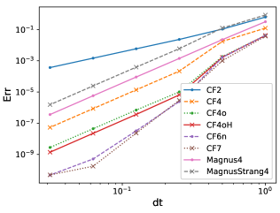
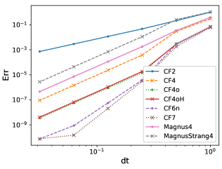
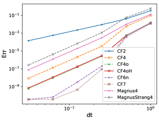
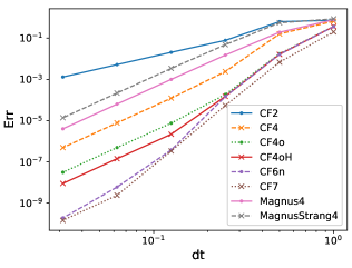
Figure 8: $2\times 4$ geometry, equidistant time-stepping. Error as a function of the step-size for $\omega=3.5$ (top row), $\sigma_{p}=1$ (top left) and $\sigma_{p}=4$ (top right), and for $\sigma_{p}=2$ (bottom row), $\omega=1.75$ (bottom left) and $\omega=7$ (bottom right).

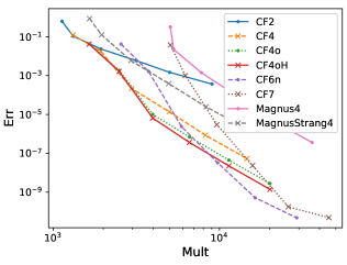
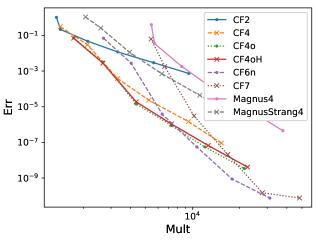
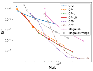
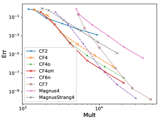
Figure 9: $2\times 4$ geometry, equidistant time-stepping. Error as a function of matrix–vector multiplications for $\omega=3.5$ (top row), $\sigma_{p}=1$ (top left) and $\sigma_{p}=4$ (top right), and for $\sigma_{p}=2$ (bottom row), $\omega=1.75$ (bottom left) and $\omega=7$ (bottom right).

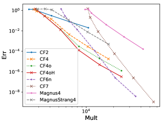
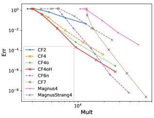
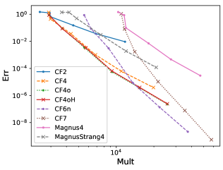
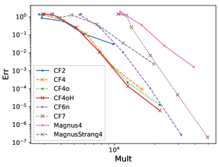
Figure 10: $4\times 3$ geometry, equidistant time-stepping. Error as a function of matrix–vector multiplications for $\omega=3.5$ (top row), $\sigma_{p}=1$ (top left) and $\sigma_{p}=4$ (top right), and for $\sigma_{p}=2$ (bottom row), $\omega=1.75$ (bottom left) and $\omega=7$ (bottom right).

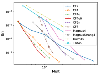
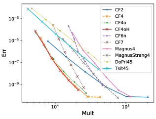
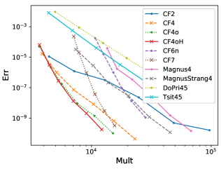
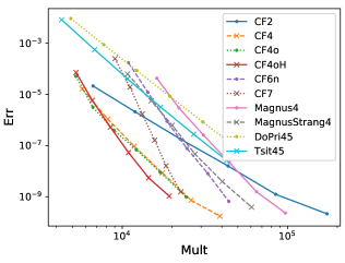
Figure 11: $2\times 4$ geometry, adaptive time-stepping. Error as a function of matrix-vector multiplications for $\omega=3.5$ (top row), $\sigma_{p}=1$ (top left) and $\sigma_{p}=4$ (top right), and for $\sigma_{p}=2$ (bottom row), $\omega=1.75$ (bottom left) and $\omega=7$ (bottom right).

References

- [1] P. Werner, K. Held, M. Eckstein, Role of impact ionisation in the thermalization of photoexcited mott insulators, Phys. Rev. B 90 (2014) 235102.
- [2] M. Innerberger, P. Worm, P. Prauhart, A. Kauch, Electron-light interaction in nonequilibrium – exact diagonalization for time dependent Hubbard Hamiltonians, arXiv e-prints (2020) arXiv:2005.13498arXiv:2005.13498.
- [3] E. Assmann, P. Blaha, R. Laskowski, K. Held, S. Okamoto, G. Sangiovanni, Oxide heterostructures for efficient solar cells, Phys. Rev. Lett. 110 (2013) 078701. doi:10.1103/PhysRevLett.110.078701.
-
[4]
M. E. Sorantin, A. Dorda, K. Held, E. Arrigoni,
Impact ionization
processes in the steady state of a driven mott-insulating layer coupled to
metallic leads, Phys. Rev. B 97 (2018) 115113.
doi:10.1103/PhysRevB.97.115113.
URL https://link.aps.org/doi/10.1103/PhysRevB.97.115113 - [5] W. Shockley, H. J. Queisser, Detailed balance limit of efficiency of p-n junction solar cells, J. Appl. Phys. 32 (1961) 510.
- [6] L. Wang, Y. Li, A. Bera, C. Ma, F. Jin, K. Yuan, W. Yin, A. David, W. Chen, W. Wu, W. Prellier, S. Wei, T. Wu, Device performance of the Mott insulator LaVO3 as a photovoltaic material, Phys. Rev. Applied 3 (2015) 064015. doi:10.1103/PhysRevApplied.3.064015.
-
[7]
M. Nakamura, F. Kagawa, T. Tanigaki, H. S. Park, T. Matsuda, D. Shindo,
Y. Tokura, M. Kawasaki,
Spontaneous
polarization and bulk photovoltaic effect driven by polar discontinuity in
LaFeO3/SrTiO3 heterojunctions, Phys. Rev. Lett. 116 (2016)
156801.
doi:10.1103/PhysRevLett.116.156801.
URL https://link.aps.org/doi/10.1103/PhysRevLett.116.156801 -
[8]
E. Manousakis,
Photovoltaic
effect for narrow-gap mott insulators, Phys. Rev. B 82 (2010) 125109.
doi:10.1103/PhysRevB.82.125109.
URL https://link.aps.org/doi/10.1103/PhysRevB.82.125109 - [9] A. Alverman, H. Fehske, High-order commutator-free exponential time-propagation of driven quantum systems, J. Comput. Phys. 230 (2011) 5930–5956.
- [10] A. Alverman, H. Fehske, P. Littlewood, Numerical time propagation of quantum systems in radiation fields, New J. Phys. 14 (2012) 105008.
- [11] E. Hairer, C. Lubich, G. Wanner, Geometric Numerical Integration, 2nd Edition, Springer-Verlag, Berlin–Heidelberg–New York, 2006.
- [12] W. Magnus, On the exponential solution of differential equations for a linear operator, Comm. Pure Appl. Math. 7 (1954) 649–673.
- [13] A. Iserles, K. Kropielnicka, P. Singh, Compact schemes for laser-matter interaction in Schrödinger equation based on effective splittings of Magnus expansion, Comput. Phys. Commun. 234 (2019) 195–201. doi:10.1016/j.cpc.2018.07.010.
- [14] J. Hubbard, Electron correlations in narrow energy bands, Proc. Roy. Soc. London A 276 (1963) 238–257.
-
[15]
M. C. Gutzwiller,
Effect of
correlation on the ferromagnetism of transition metals, Phys. Rev. Lett. 10
(1963) 159–162.
doi:10.1103/PhysRevLett.10.159.
URL http://link.aps.org/doi/10.1103/PhysRevLett.10.159 - [16] J. Kanamori, Electron correlation and ferromagnetism of transition metals, Progress of Theoretical Physics 30 (3) (1963) 275–289.
- [17] G. Mahan, Many-particle physics, 2nd Edition, Physics of solids and liquids, Plenum Press, New York, 1993.
-
[18]
E. Pavarini, E. Koch, J. van den Brink, G. Sawatzky,
Quantum Materials:
Experiments and Theory, Vol. 6 of Modeling and Simulation,
Forschungszentrum Jülich, Jülich, 2016.
URL http://juser.fz-juelich.de/record/819465 - [19] S. Jafari, Introduction to Hubbard model and exact diagonalization, Iranian Journal of Physics Research 8, available from http://ijpr.iut.ac.ir/article-1-279-en.pdf (2008).
- [20] R. Peierls, Zur Theorie des Diamagnetismus von Leitungselektronen, Z. Phys. 80 (1933) 763–791.
- [21] J. K. Freericks, V. M. Turkowski, V. Zlatić, Nonequilibrium dynamical mean-field theory, Phys. Rev. Lett. 96 (2006) 266408.
- [22] H. Aoki, N. Tsuji, M. Eckstein, M. Kollar, T. Oka, P. Werner, Nonequilibrium dynamical mean-field theory and its applications, Rev. Mod. Phys. 86 (2014) 779.
- [23] J. Stoer, R. Bulirsch, Numerische Mathematik 2, 3rd Edition, Springer-Verlag, Berlin-Heidelberg-New York, 1990.
- [24] A. Kauch, P. Worm, P. Prauhart, M. Innerbeger, C. Watzenböck, K. Held, in preparation (2020).
- [25] S. Blanes, P. Moan, Fourth- and sixth-order commutator-free Magnus integrators for linear and non-linear dynamical systems, Appl. Numer. Math. 56 (2005) 1519–1537.
- [26] S. Blanes, F. Casas, M. Thalhammer, High-order commutator-free quasi-Magnus exponential integrators for nonautonomous linear evolution equations, Comput. Phys. Commun. 220 (2017) 243–262.
- [27] W. Auzinger, H. Hofstätter, O. Koch, An algorithm for computing coefficients of words in expressions involving exponentials and its application to the construction of exponential integrators, in: M. England, W. Koepf, T. Sadykov, W. Seiler, E. Vorozhtsov (Eds.), Computer Algebra in Scientific Computing, Vol. 11661 of Lecture Notes in Computer Science, Springer Verlag, 2019, pp. 197–214.
- [28] H. Hofstätter, Order conditions for exponential integrators, arXiv:1902.11256v1 (2019).
- [29] W. Auzinger, H. Hofstätter, O. Koch, M. Quell, M. Thalhammer, A posteriori error estimation for Magnus-type integrators, M2AN – Math. Model. Numer. Anal. 53 (2019) 197–218. doi:https://doi.org/10.1051/m2an/2018050.
- [30] S. Blanes, F. Casas, J. Oteo, J. Ros, The Magnus expansion and some of its applications, Phys. Rep. 470 (2008) 151–238.
- [31] A. Iserles, H. Munthe-Kaas, S. Nørsett, A. Zanna, Lie group methods, Acta Numer. 9 (2000) 215–365.
- [32] P. Bader, A. Iserles, K. Kropielnicka, P. Singh, Efficient methods for linear Schrödinger equation in the semiclassical regime with time-dependent potential, Proc. R. Soc. A 472 (2016) 20150733. doi:http://dx.doi.org/10.1098/rspa.2015.0733.
- [33] W. Auzinger, O. Koch, An improved local error estimator for symmetric time-stepping schemes, Appl. Math. Lett. 82 (2018) 106–110. doi:10.1016/j.aml.2018.03.001.
- [34] W. Auzinger, H. Hofstätter, O. Koch, Symmetrized local error estimators for time-reversible one-step methods in nonlinear evolution equations, J. Comput. Appl. Math. 356 (2019) 339–357. doi:10.1016/j.cam.2019.02.011.
- [35] N. Higham, Functions of Matrices. Theory and Computations, SIAM, Philadelphia, PA, 2008.
- [36] P. Singh, Sixth-order schemes for laser–matter interaction in the schrödinger equation, J. Chem. Phys. 150 (2019) 154111.
- [37] C. Moler, C. Van Loan, Nineteen dubious ways to compute the exponential of a matrix, twenty-five years later, SIAM Rev. 45 (1) (2003) 3–000.
- [38] T. Jawecki, W. Auzinger, O. Koch, Computable strict upper bounds for krylov approximations to a class of matrix exponentials and -functions, BIT 60 (2020) 157–197.
- [39] M. Hochbruck, C. Lubich, H. Selhofer, Exponential integrators for large systems of differential equations, SIAM J. Sci. Comput. 19 (1998) 1552–1574.
- [40] C. Lubich, On splitting methods for Schrödinger–Poisson and cubic nonlinear Schrödinger equations, Math. Comp. 77 (2008) 2141–2153.
- [41] J. Niesen, W. Wright, Algorithm 919: A Krylov subspace algorithm for evaluating the -functions appearing in exponential integrators, ACM Trans. Math. Software 38 (2012) 22.
- [42] Y. Saad, Analysis of some Krylov subspace approximations to the matrix exponential operator, SIAM J. Numer. Anal. 29 (1) (1992) 209–228.
- [43] J. Dormand, P. Prince, A family of embedded Runge–Kutta formulae, J. Comput. Appl. Math. 6 (1980) 19–26.
- [44] C. Tsitouras, Runge–Kutta pairs of order 5(4) satisfying only the first column simplifying assumption, Comput. Math. Appl. 62 (2011) 770–775.