EKO: Adaptive Sampling of Compressed Video Data

Abstract.

Researchers have presented systems for efficiently analysing video data at scale using sampling algorithms. While these systems effectively leverage the temporal redundancy present in videos, they suffer from three limitations. First, they use traditional video storage formats are tailored for human consumption. Second, they load and decode the entire compressed video in memory before applying the sampling algorithm. Third, the sampling algorithms often require labeled training data obtained using a specific deep learning model. These limitations lead to lower accuracy, higher query execution time, and larger memory footprint.

In this paper, we present EKO, a storage engine for efficiently managing video data. EKO relies on two optimizations. First, it uses a novel unsupervised, adaptive sampling algorithm for identifying the key frames in a given video. Second, it stores the identified key frames in a compressed representation that is optimized for machine consumption. We show that EKO improves F1-score by up to 9% compared to the next best performing state-of-the-art unsupervised, sampling algorithms by selecting more representative frames. It reduces query execution time by 3$\times$ and memory footprint by 10$\times$ in comparison to a widely-used, traditional video storage format.

1. Introduction

The advent of high-definition cameras has led to an explosion in the amount of generated video data (Clement, 2020; Siegel, 2019). Researchers have proposed several techniques for efficiently analysing video data at scale. These efforts have focused on: (1) reducing query execution time, (2) increasing query accuracy, and (3) reducing memory footprint. To accelerate query processing, researchers have proposed techniques for sampling and filtering data using lightweight models (Kang et al., 2017; Kang et al., 2018; Lu et al., 2018; Suprem et al., 2020). Another line of research has focused on techniques for reducing the memory footprint of a video database management system (VDBMS) using versioning and content-based compression (Haynes et al., 2018; Daum et al., 2020).

Challenges. Traditional video storage formats seek to store videos in a representation that is better suited for human consumption. For instance, videos are often stored using a high frame rate and compressed using a delta encoding scheme that supports random access (Wiegand et al., 2003). These design decisions are based on the assumption that visual data is mainly consumed by humans. However, this representation is not efficient when videos are primarily analysed by machines. With a high frame rate, there is significant redundancy of information across nearby frames. As shown in Figure 4, the contents of the video only evolve slightly across a span of 4 contiguous frames. This increases the memory footprint of the VDBMS and the time that it takes to decode the video (Kang et al., 2020b). For instance, a 30-minute video stored at a frame rate of 60 fps occupies 24 GB of memory after it is loaded and decoded into a series of frames in memory by the VDMS. Optimizing the compressed video representation for machine consumption would enable faster query processing and lower the memory footprint of the VDBMS.

Another challenge lies in the usability and efficacy of the sampling algorithms in the VDBMS. These algorithms suffer from two limitations. First, they often require labeled training data obtained using a specific deep learning model (Kang et al., 2018; Kang et al., 2020a; Moll et al., 2020). So, the sampling algorithm is constrained to a specific dataset. Second, they are tailored for retrieving a static number of samples from a given video. So, the algorithm needs to tuned again for fetching a different number of samples. Designing a sampling algorithm to circumvent these limitations would improve the accuracy of the VDBMS.

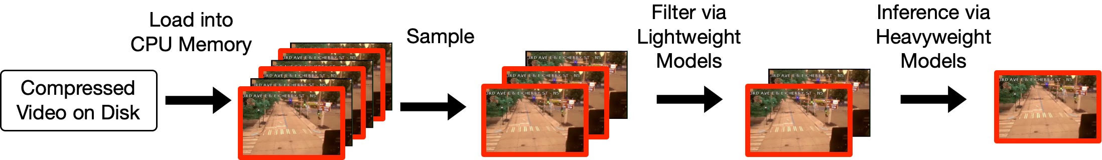
Figure 1. Video Analytics Pipeline – The key components of a pipeline for processing a query over videos.

Our Approach. In this paper, we present EKO, a storage engine for efficiently managing video data. EKO relies on two key techniques. First, it uses a novel sampling algorithm for identifying the key frames in a given video. Second, it stores the identified key frames in a compressed representation that is optimized for machine consumption with support for dynamic sampling rates. Using these two techniques, EKO improves accuracy, reduces the query execution time, and lowers the memory footprint.

EKO consists of three components: (1) Preprocessor, (2) Encoder, and (3) Decoder (illustrated in Figure 2). First, the Preprocessor identifies the key frames in the given video using a clustering algorithm. It constructs a hierarchy of these representative frames to support dynamic sampling rates. Second, the Encoder stores the key frames in a compressed representation tailored for machine consumption. Third, the Decoder efficiently retrieves a subset of frames from the compressed video based on the requirements of the Execution Engine.

Our evaluation of EKO shows that it performs up to 9% better in terms of F1-score than the next best state-of-the-art unsupervised, sampling algorithms when selecting 0.1% of the video for evaluation. The gap between EKO and other methods significantly increases as we lower the number of frames sampled. It reduces query execution time by 3$\times$ and memory footprint by 10$\times$ in comparison to a widely-used, traditional video storage format. EKO generates compressed videos that increase the storage footprint compared to traditional compressed videos by 2$\times$. But, this is still 100$\times$ smaller than that associated with storing the video as a series of frames on disk to facilitate faster query processing.

Contributions. The key contributions of this paper are:

• We motivate the need for a compressed representation tailored for machine consumption (§ 2).

• We present a clustering algorithm for identifying the key frames of a video in an unsupervised manner (§ 4).

• We introduce an adaptive sampling algorithm for efficiently decoding videos while processing queries (§ 5).

• We demonstrate that EKO reduces query execution time, improves accuracy compared to other unsupervised sampling algorithms, and significantly reduces memory footprint in comparison to a traditional storage format (§ 7).

2. Motivation & Background

We now present a motivating example that highlights the need for a machine-centric compressed representation in § 2.1. We then provide a brief overview of related work on compressing, analysing, and sampling videos in § 2.2.

2.1. Motivating Example

Consider the following query that retrieves frames with more than two cars from a traffic surveillance dataset:

⬇

SELECT frames

FROM UA_DETRAC

WHERE vehicle_type = ’car’

AND target_vehicle_count >= 2;

VDBMS	Custom Feature Extraction Network	Sampling Algorithm	Label Propagation Methodology	Distance Metric
EKO	✓	Clusterer + Frame Selector	Clusterer	L2
NOSCOPE		Thresholding		L2
TASTI	✓	FPF	KNN	L2
US		Uniform Sampling

Table 1. Video Sampling Algorithms – Qualitative comparison of sampling algorithms used in recently proposed VDBMSs.

As shown in Figure 1, a VDBMS answers this query using the following operators. First, it loads all the frames of the given video from disk to CPU memory and decodes them. Second, it samples a subset of frames from the decoded, in-memory sequence of frames. The sampling algorithm takes advantage of the fact that the contents of nearby frames in a video are similar to each other. Third, it filters out a subset of the sampled frames using a lightweight machine learning model (e.g., linear SVM (Cortes and Vapnik, 1995)). While the filtering algorithm is less accurate than a deep learning model, it lowers the query execution time by discarding a significant subset of irrelevant frames. Lastly, it moves the filtered frames from CPU memory and GPU memory and applies the heavyweight deep learning model on these frames to evaluate the predicates in the query (e.g., type of vehicles present in the frame).

It is critical to answer the queries efficiently while satisfying the accuracy requirements of the user. A naïve, uniformly-random sampling algorithm hurts query accuracy by up to 100% (§ 7.3). In contrast, if the system were to sample infrequently for higher efficiency and the target event occurs rarely in the video, then it is likely that the event goes undetected.

EKO tackles these challenges by identifying the key frames in the given video using an unsupervised algorithm. It then compresses the video in a machine-centric representation that keeps track of the key frames. Lastly, it decodes only the frames necessary for query processing to lower the I/O overhead.

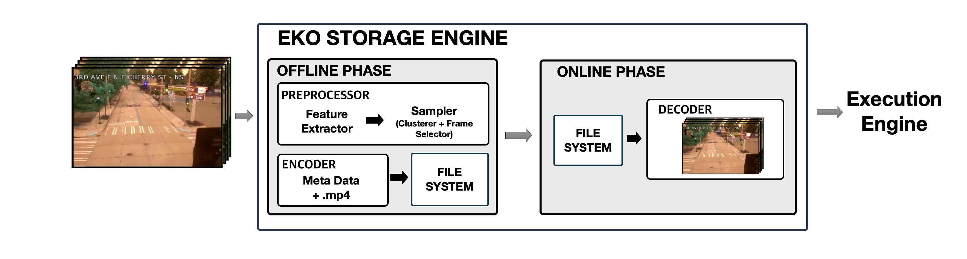
Figure 2. Architecture of EKO – EKO consists of three components. The preprocessor extracts the key frames from the given video using an unsupervised sampling algorithm. The encoder utilizes these key frames to generate a differently compressed video. The decoder allows EKO to quickly load a subset of the key frames from the compressed video on disk to CPU memory for query execution.

2.2. Background

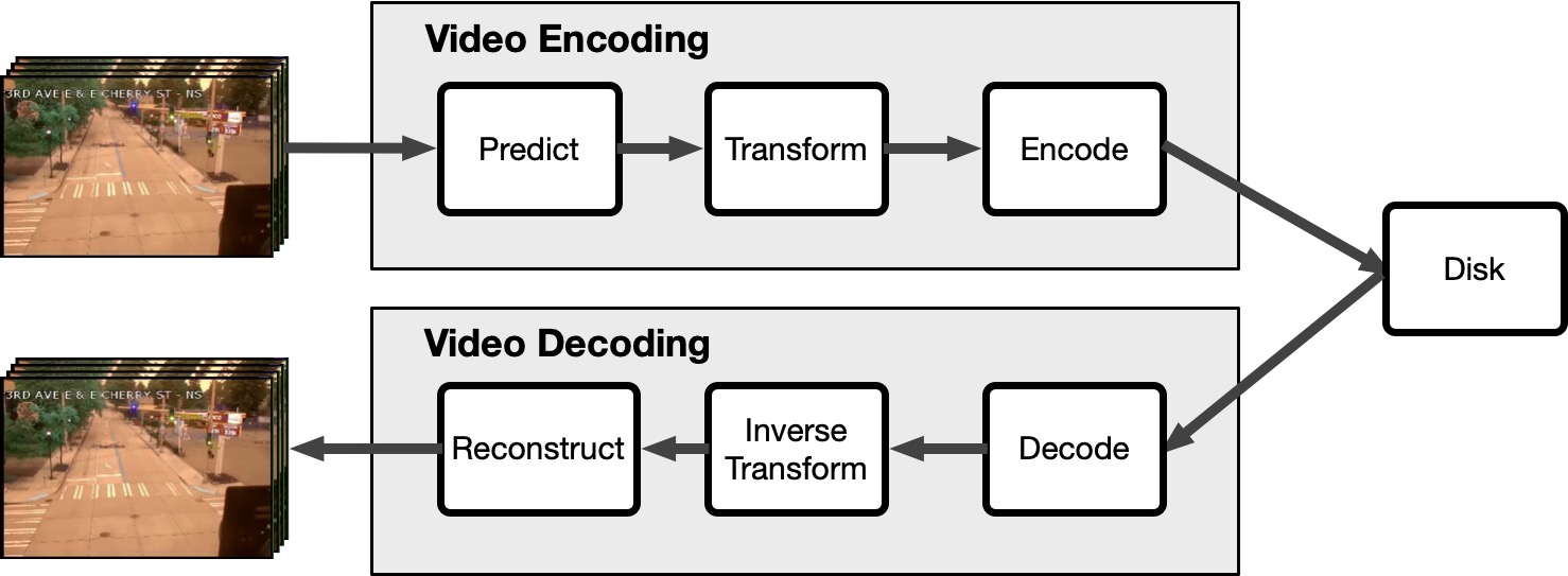
Figure 3. H.264 Video Coding Format – Steps associated with encoding and decoding H.264 video coding format.

Video compression. Video compression is centered around: (1) intra-frame, and (2) inter-frame coding. Intra-frame coding leverages correlation between pixels within the same frame. Intra-frame coding process is identical to standard image compression standards such as JPEG compression. As shown in Figure 3, it consists of the following steps: (1) prediction, (2) transformation, (3) quantization and encoding. Frames are initially divided into macroblocks (typically 16x16 pixels) and content predictions are made using surrounding macroblocks. Macroblock values are transformed using discrete cosine transform functions (DCT). The coefficients of the DCT are quantized according to the specified precision. Intra-frame coding compresses video by $3\times$ compared to raw pixel values (§ 7.6) and enables fast random access to a particular frame.

Inter-frame coding leverages the temporal redundancy between nearby frames in the video. It uses the same macroblock used for intra-frame coding. But, during the prediction step, it also uses information in previously encoded frames. The three major frame types in a compressed video are: (1) I-frames that serve as reference frames and do not require other frames for decoding, (2) P-frames require data from previous frames for decoding, and (3) B-frames require data from both previous and forward frames for decoding. We refer to P- and B-frames as delta frames since they only store the difference between nearby frames rather than each full frame. Figure 7 illustrates the differences between I and P frames. We elaborate on how EKO encodes a different set of I-frames in § 5.1.

The Encoder first determines how to best represent the current frame of interest: I- or B- or P-frame. The Encoder generates motion vectors to capture the movement in video with respect to prior frames. It calculates the difference between the prediction for the current frame and its actual contents, and encodes the difference as a residual. Inter-frame coding further decreases the storage footprint of the video by $100\times$ (§ 7.6).

Video container formats often use both intra- and inter- frame coding (e.g., AVI (avi, [n.d.]), MP4  (Pereira et al., 2002)). The downside to this approach is that random access takes time. This is because when a VDBMS seeks to extract a certain frame in the video, the decoder must first access the first frame in the group of pictures (GOP) and apply the delta calculations on top of that frame. EKO manipulates the I-frames of the video during ingestion to accelerate query processing and to lower the storage footprint.

Video analytics pipeline. As shown in Figure 1, in contemporary VDBMS systems, the query processing pipeline consists of the following components: (1) Data Loader, (2) Sampler, (3) Filter, and an (4) User Defined Function (UDF). The Data Loader migrates the video data from disk to CPU memory. It only loads the segments of the video that are required for processing the query. The Sampler is responsible for selecting a set of important frames in the loaded video. A couple of naïve sampling algorithms are: (1) uniformly sampling frames from the video, and (2) selecting the I-frames in the compressed video. Researchers have proposed sampling algorithms that better leverage the temporal redundancy of the video (Moll et al., 2020; Jiang et al., 2018; Kang et al., 2017).

UDF refers to the heavyweight deep learning model used by the VDBMS to process the query. This includes object detection (e.g., YOLO (Redmon et al., 2016)) and object classification models (e.g., VGG (Simonyan and Zisserman, 2014)). Filter are faster models compared to UDFs. However, their performance comes at the expense of a drop in accuracy. The Filter take a variety of forms ranging from traditional machine learning models (e.g., linear SVM, random forest) to specialized deep neural networks. VDBMSs leverages filters to accelerate queries with a tolerable accuracy drop (Lu et al., 2018; Anderson et al., 2019).

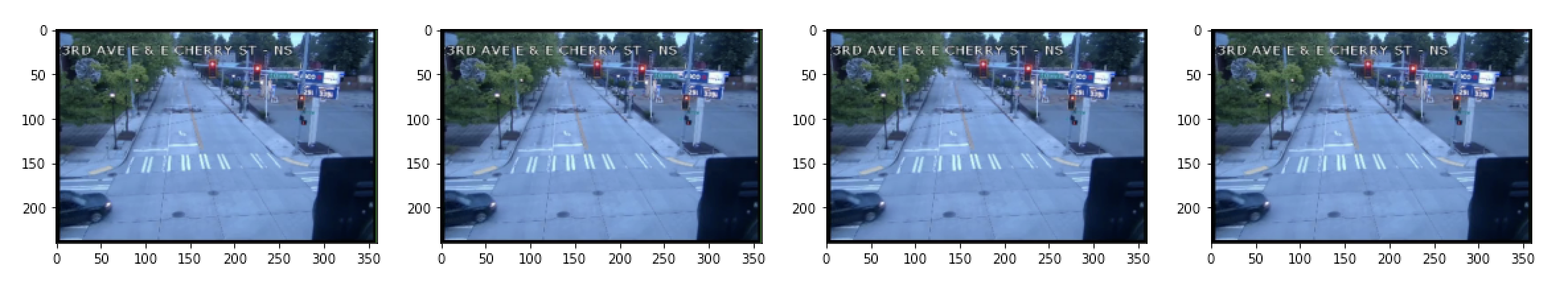
Figure 4. Temporal Redundancy – Corresponding pixels in contiguous video frames tend to take similar values. Video compression schemes exploit this temporal redundancy by only storing the differences between nearby frames rather than each full frame.

Video Sampling. VDBMSs apply sampling algorithms to leverage the temporal redundancy in videos. Depending on the sampling rate, the VDBMS may answer the query orders of magnitudes faster. BLAZEIT (Kang et al., 2018) utilizes control variates to efficiently sample video frames for LIMIT queries. EXSAMPLE (Moll et al., 2020) is tailored for queries that require detection of distinct objects. Based on the distribution of objects, it adopts a different sampling technique. These algorithms require labeled data for sampling frames.

Researchers have also presented unsupervised, sampling algorithms. NoScope (Kang et al., 2017), Tasti (Kang et al., 2020a), and EKO fall under this category. We present a qualitative comparison of these algorithms in Table 1. NoScope samples frames whenever the difference between the current frame and the previous frame exceeds a certain threshold. Since there is no specified method of propagating labels to the frames that have not been sampled, the set of queries that it can answer is limited. It does not rely on a feature extraction network to derive the features for a given image. Tasti is the closest system in terms of objectives to EKO. It leverages a custom feature extraction network based on triplet loss (Chechik et al., 2010). It selects samples using the Furthest Point First (FPF) algorithm (Rosenkrantz et al., 1977), and propagates labels using a variation of K-Nearest Neighbors (KNN) algorithm (Altman, 1992). We defer a comparison of EKO against these systems to § 7.3.

3. System Overview

The architecture of EKO is shown in Figure 2. EKO seeks to: (1) accelerate inference queries, and (2) minimize the CPU memory footprint during query processing. It automatically extracts the key frames in the given video using an unsupervised algorithm. The benefits of this design decision are twofold. First, most of the video content being created do not have labels associated with them. EKO supports such unlabeled data. Second, it exploits the innate structure of videos thereby allowing it to support a broader range of UDFs and queries.

Use Case. Consider a database with a week’s worth of video data collected from a camera deployed at a given intersection. If an urban planner is counting the number of cars passing by this intersection, EKO quickly answers this query by sampling 1% of the frames and processing them using the rest of video analytics pipeline. To facilitate efficient sampling, EKO pre-processes the video data in an offline manner to pick the most representative frames during ingestion and stores the processed videos on disk. When the user issues the query, it only decodes the top 1% of the frames that summarize the given dataset, and sends it to the Execution Engine.

Workflow. When the user loads a video into the VDBMS, EKO summarizes the given data. EKO’s Preprocessor automatically infers the optimal number of samples using the Silhouette technique (Rousseeuw, 1987). The Encoder stores the sampling results in the compressed representation. Lastly, when the user issues a query, the Decoder loads the necessary frames from the compressed video to answer the query efficiently.

Input : Decompressed video dataset $M$ (e.g., frames)
Number of samples $N$ (optional)

Output : Set of sampled frames $S$ (subset of $M$)

1

2Function Preprocess($M$, $N$):

3       $D=ExtractFeatures(M)$

4       $C=ClusterFeatures(D,N)$

5       $S=SelectFrames(C)$

6      

7      return $S$

8Function ExtractFeatures($M$):

9       $FE=InitFeatureExtractionNetwork()$

10       for $M_{\_}i\in M$ do

             // Downsample the video frames using EKOD

11             $D_{\_}i=FE(M_{\_}i)$

12            

13      return $D$

14Function ClusterFeatures($D$, $N$):

       // Compute connectivity matrix to enforce explicit temporal constraint

15       $conn=ComputeConnectivity(D)$

       // Compute optimal number of samples using heuristics if not given

16       if $N$ is $NONE$ then

17             $N=ComputeOptimalN(D)$

18            

19      else

20            

      // Cluster based on features and connectivity

21       $C=Cluster(D,conn,N)$

22      

23      return $C$

24Function SelectFrames($C$):

       // Sample a frame from each cluster

25       for $C_{\_}i\in C$ do

26             $S_{\_}i=SelectTemporalMiddleFrame(C_{\_}i)$

27            

28      return $S$

Algorithm 1 Algorithm for sampling frames in a video dataset.

4. Preprocessor

The Preprocessor is based a novel, unsupervised clustering algorithm that is tailored for the given video dataset and that iteratively converges to an optimal set of cluster centers. It finds the set of representative frames from the given video that is used for subsequent query processing. The benefits of the Preprocessor are twofold. First, it outperforms other widely-used sampling algorithms (e.g., uniform sampling), especially for queries focusing on rare events. Second, it does not require labeled video data.

As shown in Figure 5, while processing the selected frames using the User Defined Function, the Execution Engine propagates the binary label assigned to a sampled frame to the other frames within the same cluster (that were not selected by the sampling algorithm). As illustrated in Figure 2, the Preprocessor consists of two components: (1) Feature Extractor, and (2) Sampler. We next describe these components in detail.

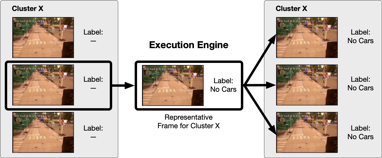
Figure 5. Label Propagation Method – The Execution Engine propagates the binary label assigned to a sampled key frame to the other frames within the same cluster. For instance, if the key frame contains no cars, it assumes that the other frames in the same cluster also contain no cars.

4.1. Feature Extractor

Algorithm 1 outlines the steps for choosing the representative frames. The Preprocessor first downsamples the frames in the given video before applying the clustering algorithm to circumvent the curse of dimensionality (Bellman, 1954). With high dimensional data, the L2 distance metric used for clustering the data does not accurately capture the underlying distribution. Lowering the dimensionality of the data increases the efficacy and the efficiency of the clustering algorithm. Since the complexity of the clustering algorithm grows quadratically with the number of dimensions ($n$), reducing $n$ by 2$\times$ leads to a 4$\times$ speedup.

Challenges. Choosing the appropriate downsampling algorithm is a non-trivial task. As we later show in § 7.3, the downsampling algorithm has a significant effect on the accuracy of the query. The Feature Extractor must satisfy the following objectives:

• The Feature Extractor must not only consider the raw pixel content of the frames, but also take the key objects themselves into consideration.

• The Feature Extractor must consider the temporal dynamics of the video.

• The downsampling algorithm must work well with the subsequent clustering algorithm.

The reason why we need to focus on the objects is because the queries we target are centered around them. If the Feature Extractor only considers the raw pixel content for clustering, it has a higher likelihood of not capturing the crucial features.

Our Approach. Feature Extractor uses a modified VGG16 (Simonyan and Zisserman, 2014) network for feature extraction. It implicitly enforces an ordering constraint to force similar frames in the video to be grouped together after the clustering algorithm. To embed this constraint, it fine-tunes the pretrained VGG16 network as outlined in Algorithm 2. After extracting the features, it passes them to the clustering algorithm. While training the model, it uses the labels generated from executing the clustering algorithm from the previous iteration to compute the loss. Feature Extractor uses the Adam optimizer for gradient-based optimization of the network.

EKO’s training procedure is a variant of the canonical iterative parameter update technique. In particular, it is related to Deep Embedded Clustering (DEC) (Xie et al., 2016). While DEC is tailored for images, EKO focuses on sampling from videos. So, it uses a different clustering algorithm. While DEC utilizes K-means for deriving the groups and to compute the loss, EKO relies on hierarchical clustering (Ward Jr, 1963). Furthermore, EKO’s clustering algorithm enforces explicit temporal constraints, thereby altering the behavior of the Feature Extractor.

Input : Decompressed video dataset $M$ (e.g., images)

Number of samples $N$ (optional)

Iteration limit $I$ (default value: 100)

Output : Set of sampled frames $S$ (subset of $M$)

1

2Function TrainFeatureExtractor($M$, $N$):

3      

4      $I_{\_}{curr}$ = 0

5       while $I_{\_}{curr}\leq\mathcal{I}$ do

6            

7            $D=ExtractFeatures(M)$

8             $C=ClusterFeatures(D,N)$

9             for $D_{\_}i\in D$ do

                   // For the current features, find the selected frame within the cluster

10                   $S_{\_}j=FindClusterRep(D_{\_}i)$

                   // Compute the distance between the selected frame and current frame

11                   $L=ComputeDist(D_{\_}i,S_{\_}j)$

                   // Perform backpropagation to update the network’s parameters

12                   $L.Backprop()$

13      return $\mathcal{S}$

Algorithm 2 Algorithm for training the feature extractor.

4.2. Sampler

As shown in Algorithm 1, the Sampler takes the downsampled frames returned by Feature Extractor as input. It first clusters these frames together and then selects a representative frame from each cluster. We modify the canonical hierarchical clustering algorithm (Ward Jr, 1963). First, EKO explicitly adds a temporal constraint to group contiguous frames together. Second, EKO automatically derive the required number of clusters by tailoring the silhouette method (Rousseeuw, 1987). Third, we empirically show that it is important to select the middle frame of each temporal cluster as the representative frame.

Temporal Constraint. While the Feature Extractor chooses important features needed to understand the content of the video frames, we found that it is important to explicitly add a temporal constrain to group contiguous frames together. This improves the efficacy of the Sampler (§ 7.7). Consider the movement of the car in Figure 4. If a frame at timestamp $t$ contains one car, then it is likely that the frames at timestamps $t-1$ and $t+1$ also contain one car. By explicitly enforcing the clustering algorithm to consider groupings of contiguous frames together, Sampler fully leverage the temporal redundancy in videos.

Dynamic Sample Selection. EKO allows the user to specify the number of samples required for answering the query. During ingestion, the Sampler computes the hierarchical tree specifying the clusters and caches it. Using this cached tree, it determines the cluster formations for the desired number of samples. Besides the already selected representative frames, it obtains additional samples by selecting frames that are closest to the temporal median of each cluster. As we show in § 7.3, these samples deliver higher accuracy compared to uniform sampling over the already selected representative frames.

Frame Selection. After determining the optimal number of clusters and clustering the downsampled datapoints, Sampler is left with the task of selecting the representative frames of each cluster that will be then be sent to the Execution Engine. We take the temporal redundancy of videos into consideration in the frame selection decision. In particular, we assume that the probability that frames at timestamps $t$ and $t+1$ are likely to have the same label compared to that of frames separated by more than 10 frames. So, if Sampler must only pick one frame from each cluster, then selecting the middle frame increases the likelihood that the other frames in the cluster share the same label as the selected frame. We show the importance of picking the middle frame in § 7.8.

4.3. Theoretical Analysis

We now present a theoretical analysis of the clustering algorithm used by EKO. Consider a set of $n$ points in the set $\{x_{\_}i\in X\}^{n}_{\_}{i=1}$ that we seek to group together into $k$ clusters. We assume that for every given dataset $X\in\mathbb{R}^{d_{\_}x}$, there exists an underlying latent space $Z\in\mathbb{R}^{d_{\_}z}$ that is optimal for sampling. $X$ and $Z$ differ in that the latter dataset focuses more on the objects in the frames that are relevant for the video analytics queries. While we cannot directly derive $Z$, we seek to learn $\hat{Z}\in{\mathbb{R}^{d_{\_}{\hat{z}}}}$ that approximates $Z$. We denote the transformation function by $h_{\_}\theta:X\rightarrow\hat{Z}$, where $\theta$ are learnable parameters.

Characteristics of Latent Space. We now list the desired characteristics of $\hat{Z}$. First, $d_{\_}{\hat{z}}<<d_{\_}x$. Reducing the dimensionality of the dataset will allow EKO to circumvent the curse of dimensionality. Next, if frames are temporally close to each other, they should be close to each other in the latent space as well. This property allows us to leverage the temporal redundancy of videos. Lastly, every cluster in the latent space must be dense. This ensures that frames with similar content are grouped together, thereby increasing the likelihood of these frames being grouped together by the clusterer.

Learning the Transformation Function. To learn the transformation function $h_{\_}\theta$ in an unsupervised manner, we impose explicit and implicit constraints on the Feature Extractor and its training process. We begin with a pre-trained VGG16 network so that the Execution Engine may leverage the features returned by this network. A deep learning network learns a function $f(x)$ of the form $f(x)=g(h_{\_}\theta(x))$. Here, $h_{\_}\theta(x)$ is the feature extraction network and $g(x)$ is the labeling function.

We constrain $h_{\_}\theta$ to match the underlying distribution $\hat{Z}$ in two ways. First, we augment $\{\hat{z}_{\_}i\in{\hat{Z}}\}_{\_}{i=1}^{n}$ by concatenating the temporal location of the frame and downsizing the output of the VGG16 network using an fully connected layer. This imposes an implicit temporal connectivity constraint on the points in the latent space. By downsizing the output of the VGG16 network, EKO chooses the key features, and reduces the dimensionality of the dataset (i.e., $d_{\_}{\hat{z}}<<d_{\_}x$). Second, we impose an additional explicit constraint for temporal connectivity. To meet the desired characteristics of the latent space, we seek to find $\theta$ that minimizes the following objective function:

$$\min_{\_}{\theta}\Sigma_{\_}{i=1}^{n}(f_{\_}\theta(x_{\_}i)-f_{\_}\theta(c(x_{\_}i))^{2})$$

In other words, EKO tries to minimize the difference between the features of a given video frame and that of the representative frame of the cluster to which it belongs.

5. Video Encoder and Decoder

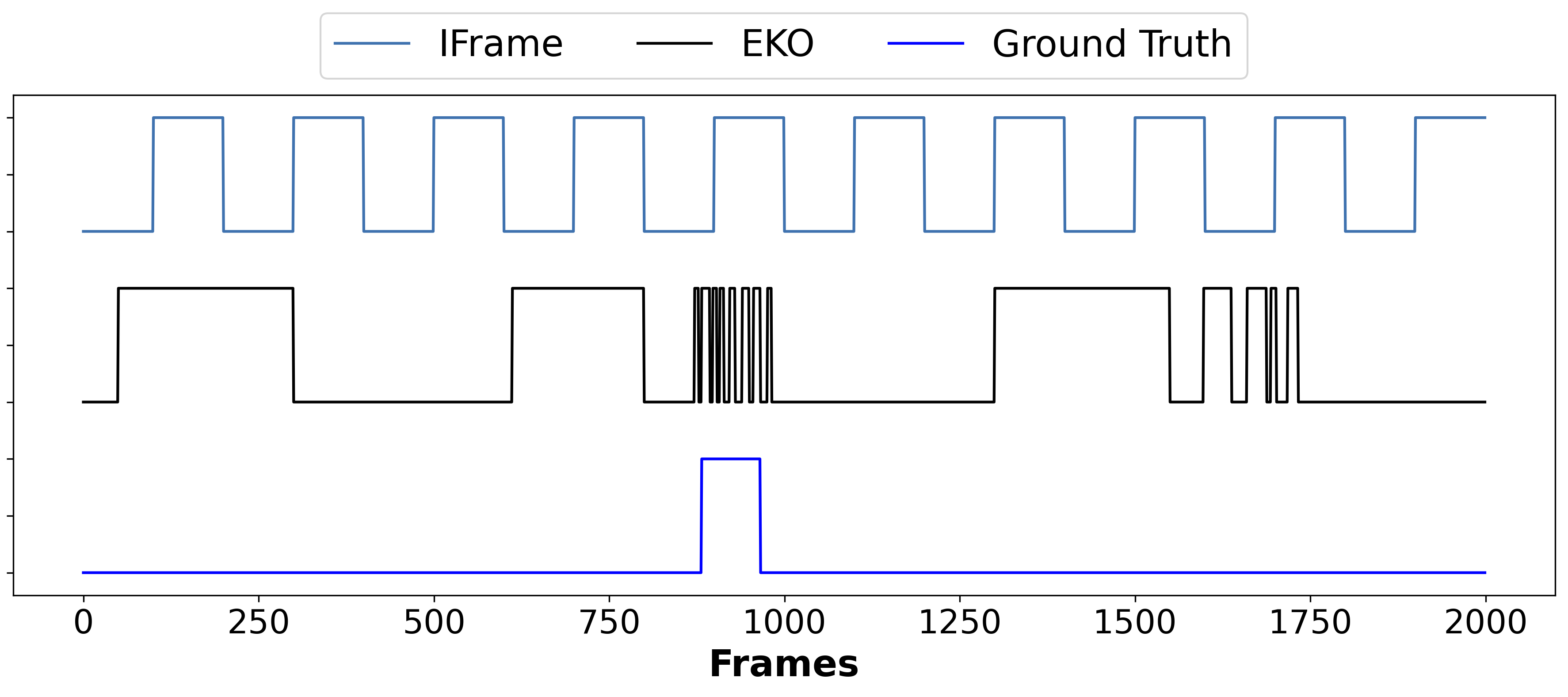
Figure 6. Cluster Boundaries – We represent each cluster by a transition along the sequence of frames. EKO adjusts the cluster boundaries based on the contents of the frames.

In this section, we first explain why canonical I-frames do not meet the requirements of the VDBMSs in § 5.1. We then discuss how the frames sampled by EKO are different from I-frames in § 5.2. Lastly, we discuss how EKO encodes and decodes video in  § 5.3.

5.1. Canonical I-Frames

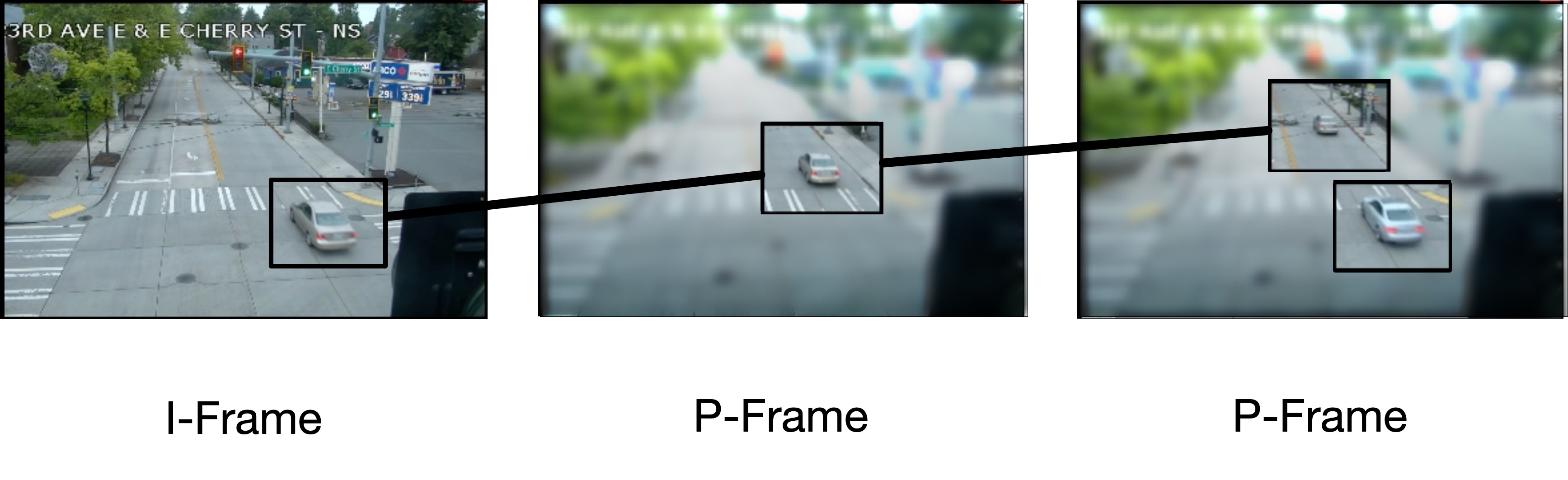
Figure 7. I- and P-frames – Visualization of intra-coded (I) and predicted (P) frames in a compressed video.

In this paper, we focus on the H.264 video compression standard. As shown in Figure 7, within a GOP, the I-frame is always the first frame. Subsequent P- and B-frames refer back to this I-frame for decoding (§ 2.2). The number of frames within a single GOP depends on multiple factors, including: (1) frame rate, and (2) constant rate factor. Typically, videos with higher frame rate have a GOP with around 250 frames. Since I-frames do not refer back to any frame, it takes less time to decode a random I-frame as opposed to other types of frames. So, EKO seeks to use I-frames for processing the query. In particular, the Execution Engine propagates the labels returned by the object detector on an I-frame to other nearby frames within the video.

Challenges. The I-frames chosen by a canonical Encoder do not satisfy the requirements of the Execution Engine. If EKO were to use them for processing the query, the drop in query accuracy is significant (§ 7.3). The reasons for this is twofold. First, the canonical I-frames do not take the dynamics of the video into consideration. The size of the GOP is hard-coded to be a small constant (e.g., 250 frames) to facilitate faster retrieval of other frames within the GOP. Since I-frames typically occur at the beginning of each GOP, this is equivalent to taking uniformly random samples from the video. This approach does not work well for queries focusing on rare events. Second, as we discussed in § 4, the representative frame should be the middle frame of the group (as opposed to the first frame). This increases the likelihood that the other frames in the group share the same label as the selected frame. Given these constraints, the Encoder in EKO picks a different set of frames, as described in § 4.2, to be the I-frames in the compressed video.

5.2. Sampled Frames

We now examine the differences between the traditional I-frames and the frames sampled by EKO. Since the Encoder uses these sampled frames as I-frames in the re-encoded video, we examine the differences between these two set of frames. We focus on the query shown in § 2.1 for this analysis. We consider a dataset with 100 K frames and generate 1000 clusters. We compare the groupings with traditional I-frames (i.e., GOPs) and the clusters generated in EKO. We compute inter-cluster metrics to examine the relevance of frames grouped together. Unlike EKO, the locations of the I-frames are fixed and do not take the activity in the video into consideration. So, the clusters are uniformly sized. In contrast, EKO generates clusters that exhibit a high variance in cluster size.

	Inter Cluster Statistics
	Iframe	EKO
Mean	100	100
Median	100	26.5
Std	0	120
Min	100	2
Max	100	706

Table 2. Comparison of traditional I-frames and EKO– Inter-cluster statistics associated with the clusters generated by a traditional encoder and EKO’s encoder.

The results are shown in Table 2. With traditional I-frames, the standard deviation of the cluster size is 0. In contrast, with EKO, the standard deviation of the cluster size is 120. This is because EKO adjusts the cluster boundaries based on the variation in the contents of the video. The benefits of this technique is more prominent when the query is evaluated using a fewer number of frames. Figure 6 illustrates the differences in the generated cluster boundaries. While groupings generated using traditional compression is static, EKO dynamically adjusts the clusters. Due to correlation between changes in the contents of the video and changes in the ground truth label, EKO delivers higher accuracy than traditional I-frames.

5.3. Encoding and Decoding

EKO leverages the widely-used ffmpeg library (Tomar, 2006) for manipulating the video. In particular, it uses the x264 codec to directly configure a custom set of frames returned by Sampler as the I-frames in the re-encoded video. It uses ffmpeg in this manner:

⬇

ffmpeg -i src -force_key_frames T dst -y

Here, $T$ represents the indices of the sampled frames within the original video. $src$ and $dst$ represent the filenames of the original video and re-encoded video, respectively. While this re-encoding allows EKO to improve query accuracy, it also increases the storage footprint of the video by 80% on average (§ 7.6).

EKO uses a custom Decoder that works in tandem with the Encoder. Based on the query, it either decodes a subset of the I-frames or the entire video. We empirically show that the Decoder takes up to 10$\times$ less time to load a subset of frames picked by the Sampler in comparison to a canonical Decoder operating on the original video (§ 7.5).

6. Implementation

We implemented EKO in Python 3. The Execution Engine utilizes the Pytorch framework (v 3.7.6) for inference using deep learning models. The Encoder and Decoder leverage the ffmpeg framework (v 4.3) for compressing and decompressing videos. EKO analyzes videos in two stages.

• In the offline stage, the Preprocessor first loads the video using the OpenCV framework (v 4.2.0). It then extracts key features from the video using the Pytorch framework. Next, the Sampler takes the downsampled frames and applies a variant of the agglomerative clustering algorithm in the scikit-learn library (v 0.23.1). In particular, it uses the ward linkage criterion to minimize the variance of the clusters being merged. The Sampler then selects a set of representative frames from these clusters. These samples are passed on to the custom Encoder. The Encoder re-encodes the video to embed the sampled frames as I-frames to facilitate faster retrieval of these frames by the Execution Engine during query processing.

• In the online stage, the Execution Engine requests the Decoder to return a subset of sampled frames. The custom Decoder efficiently retrieves these frames from the re-encoded video. Lastly, the Execution Engine applies inference on these representative frames. It then propagates the labels returned by the deep learning on each representative frame to other frames within the same cluster in the the re-encoded video.

7. Experiments

In our evaluation, we illustrate that:

• EKO delivers accurate results comparable to other sampling algorithms (§ 7.3).

• EKO’s components contribute to the overall improvement in latency and accuracy (§ 7.4).

• EKO executes queries up to 27$\times$ faster than traditional efficient sampling algorithms (§ 7.5).

• EKO lowers the storage footprint by 100$\times$ compared to a canonical storage format (§ 7.6).

• We conduct a sensitivity analysis of key parameters (§ 7.7, § 7.8).

7.1. Evaluation Metrics

Latency. We measure the time it takes for EKO to load in the video from disk and to process the query using the Execution Engine (Kang et al., 2020b).

Accuracy. To evaluate the accuracy of the sampling algorithms, we use a label propagation technique. In particular, EKO propagates the labels assigned by the User Defined Function to the sampled frame $X$ to other frames that are temporally close to $X$ in the video. We compare these labels against the ground truth to measure precision and recall metrics.

7.2. Experimental Setup

Q1	⬇ SELECT frames FROM Seattle WHERE vehicle_type = ’car’ AND target_vehicle_count >= 1;
Q2	⬇ SELECT frames FROM Seattle WHERE vehicle_type = ’car’ AND target_vehicle_count >= 2;
Q3	⬇ SELECT frames FROM UA-DETRAC WHERE vehicle_type = ’car’ AND target_vehicle_count >= 2;
Q4	⬇ SELECT frames FROM UA-DETRAC WHERE vehicle_type = ’car’ AND target_vehicle_count >= 3;
Q5	⬇ SELECT frames FROM UA-DETRAC WHERE vehicle_type = ’van’ AND target_vehicle_count >= 1;

Table 3. Queries used for evaluating EKO.

Video Name	Object Name	Object Count	Resolution	FPS	# of Eval Frames	# of TRUE Frames	% of TRUE Frames
UA-DETRAC	CAR	1	960x540	25	83791	80744	96.36%
UA-DETRAC	CAR	2	960x540	25	83791	75249	89.8%
UA-DETRAC	CAR	3	960x540	25	83791	66485	79.3%
UA-DETRAC	VAN	1	960x540	25	83791	25630	30.5%
Seattle	CAR	1	728x478	60	100k	20731	20.73%
Seattle	CAR	2	728x478	60	100k	1801	1.8%

Table 4. Datasets – The key properties of the datasets used in our evaluation. We list the number of evaluated frames and the percentage of frames containing target object (i.e., number of TRUE frames).

Datasets and Queries. We evaluate EKO on two datasets: (1) UA-DETRAC (Wen et al., 2020), and (2) Seattle (sea, [n.d.]). The key properties of these traffic-surveillance datasets are summarized in Table 4. UA-DETRAC consists of numerous short traffic camera videos (each of one minute duration). The latter dataset is a 30 minute long video of a traffic intersection in Seattle.

We use the queries shown in Table 3 to evaluate EKO and other sampling algorithms. We use SSD (Liu et al., 2016) as a reference inference model. We rank all the algorithms based on how well the labels that they assign to the frames in the video compare against those assigned by SSD. We use the label propagation technique shown in Figure 5.

Sampling Algorithms. We compare six sampling algorithms in our evaluation: (1) No-Sampling, (2) I-Frame, (3) Uniform, (4) NoScope, (5) Tasti, (6) EKO-VGG, and (7) EKO. Here, No-Sampling refers to disabling the sampling optimization (i.e., evaluating all the frames of the video). It serves as an upper bound on accuracy (and a lower bound on latency). I-Frame refers to using the original I-frames picked by the x264 video compression algorithm (VideoLAN, [n.d.]). Since the I-frame always comes at the beginning of the GOP, we propagate the label assigned to this frame to the latter B- and P-frames within the same GOP. Uniform refers to picking one frame out of every $k$ frames depending on the number of required frames.

NoScope samples frames based on detecting difference between a predefined frame and current frame. While two different methods are mentioned in the paper for determining the predefined frame, we use the method that detects the difference against an earlier frame of $t_{\_}{diff}$ seconds in the past.  (Kang et al., 2017). Tasti uses triplet loss on labeled video data to derive features from the video frames. The system then applies furthest point first (FPF) algorithm (Gonzalez, 1985) and a variant of K nearest neighbors (Altman, 1992) for propagating the labels to the remainder of the frames. Since we focus on the unsupervised setting, we use the pretrained version of the TASTI (referred to as TASTI-PT in (Kang et al., 2020a)).

EKO utilizes all the optimizations outlined in this paper including: (1) a custom feature extractor, (2) temporal constraint, (3) middle frame selection, and (4) a custom encoder and decoder. In contrast, EKO-VGG uses all of these optimizations except that it utilizes a pre-trained VGG-16 network. Unless specified otherwise, all the sampling algorithms are configured to pick the same number of frames for a fair comparison.

Hardware Environment. We perform the experiments on a server with these specifications:

• CPU: 16 Intel(R) Xeon(R) Gold 6134 @ 3.20GHz

• GPU: 4 Geforce RTX 2080 Ti

• RAM: 385 GB

SSD runs at 30 fps on one RTX 2080 Ti GPU in this server.

7.3. Query Accuracy

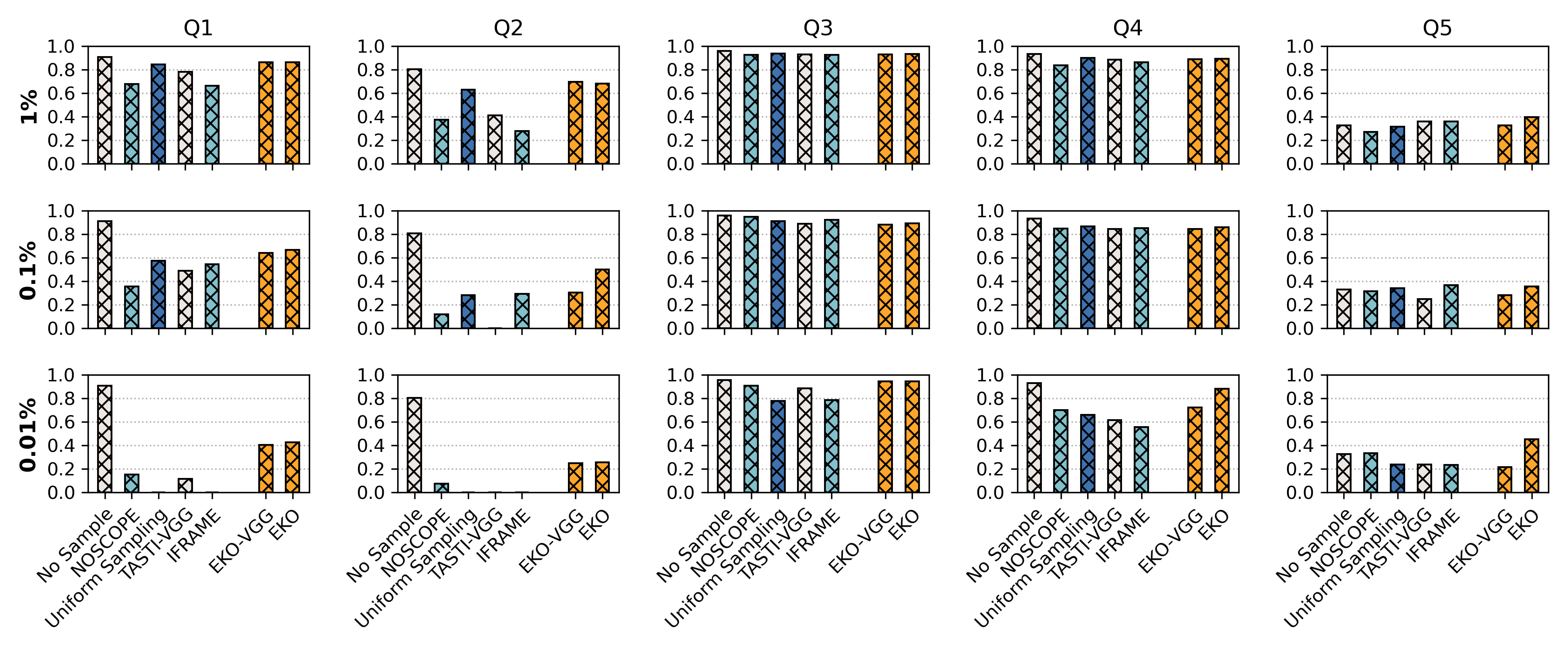
Figure 8. Accuracy – Comparison of the F1-score of different sampling algorithms across different queries. EKO strikes a balance between precision and recall metrics to achieve a high F1-score.

We first examine the end-to-end accuracy of EKO’s unsupervised, dynamic sampling algorithm outlined in § 4. We compare it against the other sampling algorithms listed in § 7.1. In this experiment, EKO first loads all of the frames into memory and then selects a subset of frames using the given sampling algorithm. It then sends those frames to the Execution Engine that runs inference using SSD (Liu et al., 2016). Lastly, the Execution Engine propagates the output label for the sampled frame to other frames in the same cluster using the method illustrated in Figure 5.

Selectivity. We vary the selectivity of the sampling algorithm (i.e., the number of samples picked) from 1% to 0.01%. For example, with a dataset of 100 K frames and selectivity of 1%, each algorithm is tailored to pick 1 K frames. We configure all the algorithms to return the same number of samples to ensure a fair comparison. We quantify query accuracy by measuring the F1-score. It is important to strike a balance between the precision and recall metrics for a given sampling algorithm to work well for diverse queries. We compare the efficacy of the algorithm against No-Sampling.

We first configure the selectivity of all the algorithms to 1%. The results shown in Figure 8. The most notable observation is that EKO’s F1-score only drops by 0.12 F1-points compared to No-Sampling. It is consistently better or on par with the second best sampling algorithm for each query.

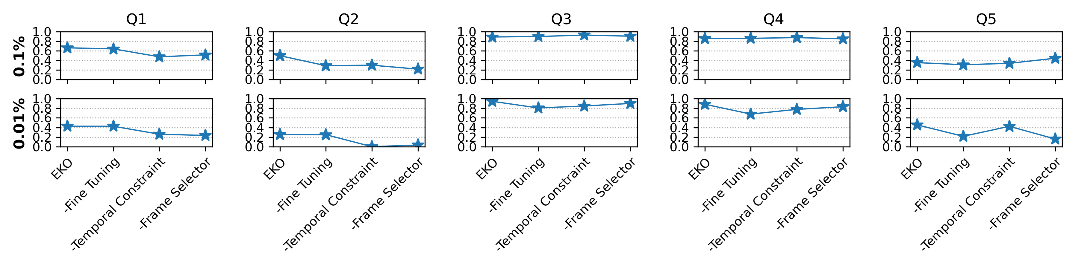
Figure 9. Ablation Study – Impact of different optimizations in EKO on accuracy. We disable optimizations one at a time: (1) feature extractor, (2) frame selector, ands (3) temporal constraint.

On Q1, EKO outperforms Uniform by 0.02 and Tasti by 0.18 points. The reasons are twofold. First, it picks a more representative set of frames that are not uniformly spread across the video. Second, it enforces a temporal constraint that improves the relevance of frames mapped to the same cluster.

On Q3, the difference between the sampling algorithms is minimal. For instance, compared to Q1, the gap between EKO and Uniform reduces from 0.02 to 0.0. This is because the frequency of the target object in this dataset is high. So, it is a relatively easier query to answer. Even if the sampling algorithm picks a less representative frame, it is likely that even this frame will contain the target object. So, the impact of the sampling algorithm on F1-score is minimal.

On Q5, EKO outperforms the No-Sampling baseline by 0.07 points. We attribute this to the comparatively low accuracy of SSD model on this query. The query focuses on a van object that is harder to detect. EKO picks a robust, representative subset of frames that reduces noise, thereby enabling it to outperform No-Sampling.

EKO outperforms EKO-VGG on average by 10% across all queries. This is because the fine-tuned network allows EKO to better extract features. The gap between EKO and EKO-VGG increases when we reduce the number of samples that they must pick.

Impact of Selectivity. As shown in Figure 8, we observe that the drop in EKO’s accuracy is minimal when we select fewer samples to process the query. When the selectivity is reduced from 1% to 0.01%, EKO’s F1-score only drops by 9%. In contrast, accuracy of Uniform and Tasti drops by 53% and 26%, respectively. We attribute this difference to the features generated by the network in EKO and its dynamic sampling algorithm.

The accuracy gap between EKO and No-Sampling decreases as we increase the number of samples. On Q2, the gap shrinks from 68% to 38% when selectivity is increased from 0.01% to 1%. This is because Q2 focuses on a rare event (i.e., frames in the Seattle dataset with more than two cars). When the selectivity is reduced to 0.01%, the difference between EKO and Uniform is more prominent.

Complexity of Query. The complexity of the query depends on: (1) the frequency of occurence of the target object, and (2) the characteristics of the dataset. For instance, while the object of interest in Q5 (i.e., van) appears more frequently compared to that in Q1 (car), all of the sampling algorithms find it hard to pick representative frames. The reasons are twofold. First, it is harder for the User Defined Function to detect vans as opposed to cars. This is why the F1-score of the No-Sampling algorithm is 64% lower on Q5 compared to that in Q1. Second, the UA-DETRAC dataset’s environment is more complex compared to that of the Seattle dataset. The frames in the former dataset contain both vans and cars. So, the sampling algorithm must carefully discriminate between the movement of these objects. Furthermore, this dataset consists of a collection short video clips focused on different traffic intersections. So, it exhibits more significant variation in object movement compared to the Seattle dataset that is a single long video focused on the same traffic intersection.

7.4. Ablation Study

We next examine the impact of different optimizations in EKO on accuracy. EKO uses three optimizations: (1) a custom feature extractor, (2) a custom frame selector, and (3) a temporal constraint. We disable these optimizations one at a time to quantify their impact on accuracy. In this experiment, we vary the selectivity of the algorithms from 0.1% to 0.01%. Without the custom feature extractor, EKO uses a pretrained VGG-16 network (i.e., same as EKO-VGG). Without the temporal constraint, EKO uses a vanilla agglomerative ward clustering algorithm to group the frames. Without the custom frame selector, EKO picks the first frame in each cluster as the representative frame. The results are shown in Figure 9. The most notable observation is that while all the optimizations contribute to the improvement in accuracy, the temporal constraint is the most important optimization.

Feature Extraction. The impact of disabling the custom feature extractor is more significant when the algorithm must pick fewer frames. For instance, on Q5 disabling this optimization leads to an accuracy drop of 25% and 50% when selectivity is 0.1% and 0.01%, respectively. This illustrates the importance of finding more representative frames using a better feature extractor.

Temporal Constraint. The most important optimization in EKO is the temporal constraint. The impact of this optimization is most prominent on complex queries (i.e., Q1, Q2). The temporal constraint allows EKO to utilize the motion information inherently present in the video. So, the algorithm is robust enough to handle the rare events that these quries seek to find. It is less susceptible to confusing a black truck and a black car that are present in completely different sections of the video. The impact of disabling these optimizations is minimal on Q3, Q4, and Q5. The frequencies of the target objects in these queries are so high that only enabling the feature extractor and picking the middle frame is sufficient to obtain quality results. We further discuss the effect of temporal constraint in § 7.7.

Frame Selection. The impact of disabling the frame selector is most significant on Q2. This query focuses on a rare event. In this case, the middle frame is more likely to be representative of the cluster as opposed to the first frame. In constrast, on Q3, Q4, and Q5, disabling the frame selector often results in better accuracy. This is because the query focuses on a frequent event and an easier dataset. So, the Execution Engine is capable of correctly answering the query even using the first frame. We further discuss the effect of frame selection strategy in § 7.8

7.5. Execution Time

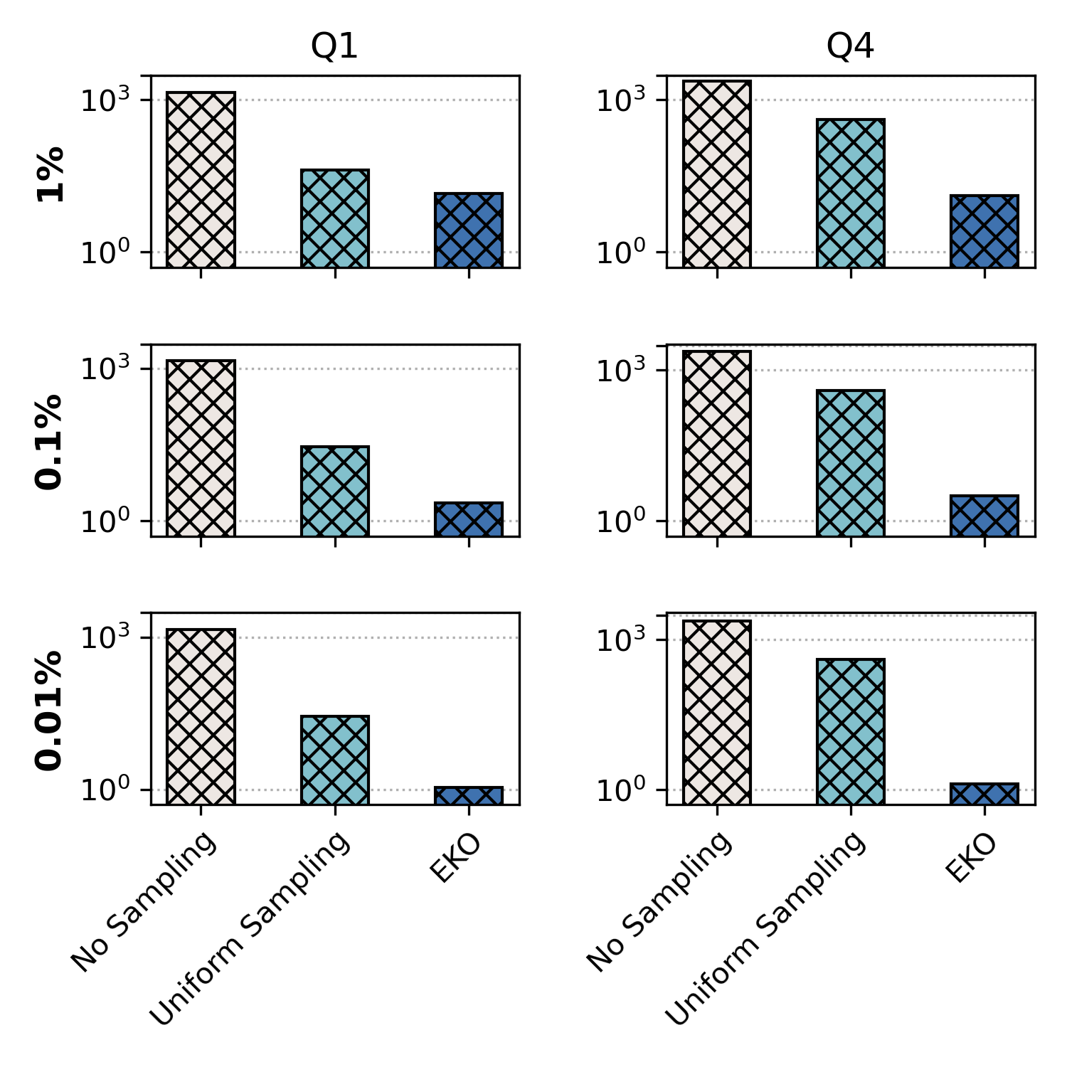
Figure 10. Execution Time – Comparison of the query processing time of different sampling algorithms.

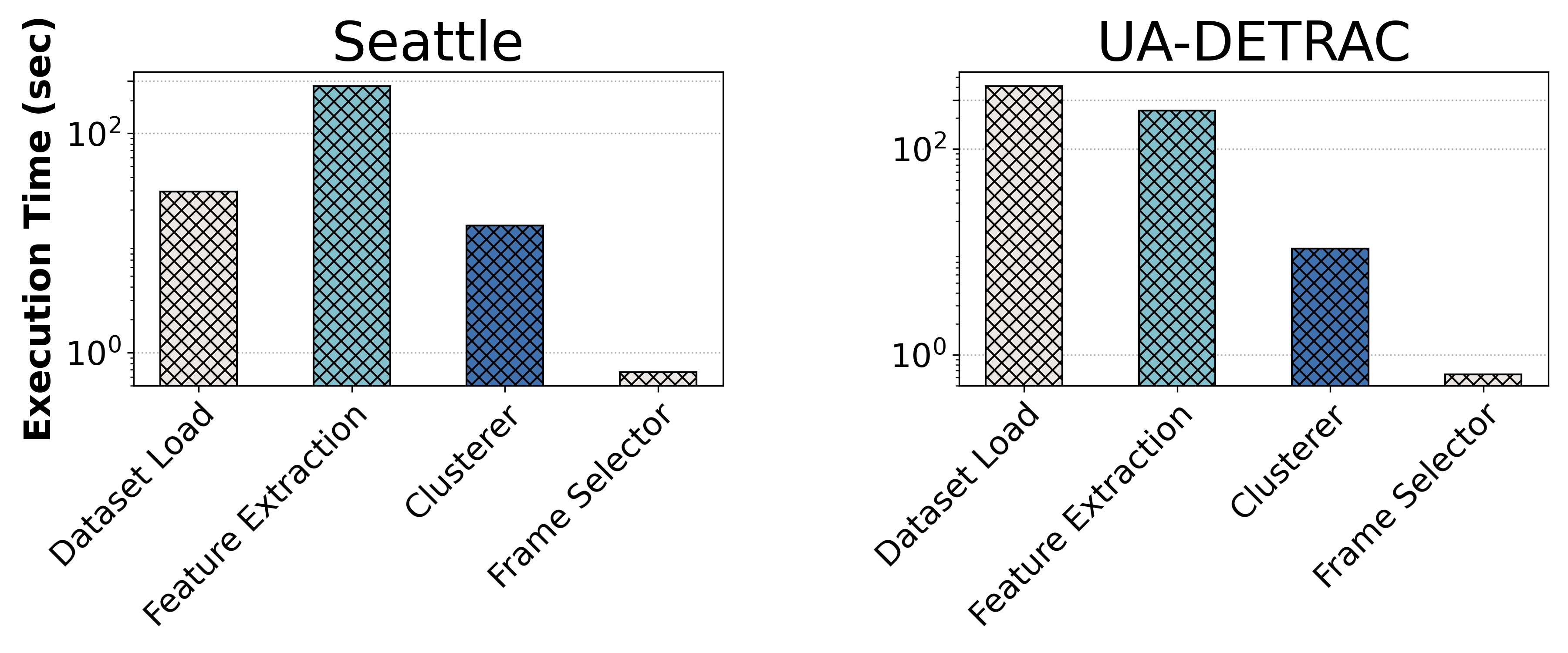
Figure 11. Preprocessing Time – Breakdown of time spent on different components of Preprocessor.

In this experiment, we compare the time taken by EKO to process queries in comparison to No-Sampling and Uniform algorithms. We focus on two representative queries: Q1 and Q3. With EKO, we assume that the Preprocessor has already constructed a compressed video with meta-data about the representative frames. Since this is an one-time cost, we do not include the pre-processing time in the results. We measure the time taken to load the sampled frames from disk to memory, and to perfor inference on those frames. We vary the selectivity of the algorithms 1% to 0.01%.

The results are shown in Figure 10. On Q1, for selectivity 1%, EKO executes the query 3$\times$ and 100$\times$ compared to Uniform and No-Sampling, respectively. Comparative speed increases as we decrease the numbers of samples used to evalute the query. We attribute this speedup to two factors. First, EKO combines the adaptive sampling algorithm and the compression scheme outlined in § 5. With both Uniform and No-Sampling, all of the frames in the video are loaded from disk to memory. In contrast, the custom decoder in EKO allows it to only load the desired number of sampled frames from the video into memory. Second, unlike No-Sampling, EKO and Uniform only run inference on the sampled frames and propagate the labels to the other frames. On average, it takes 0.3 ms and 2.7 ms to load a frame from disk to memory and to run inference on a given frame, respectively.

On Q3, EKO for selectivity 1% executes the query 31$\times$ and 180$\times$ compared to Uniform and No-Sampling, respectively. The impact of EKO is more prominent on this query focusing on the UA-DETRAC dataset. This is because this dataset is organized as a a series of images (unlike the Seattle dataset which is a compressed video format).

Impact of Selectivity. We next reduce the selectivity of the algorithms from 1% to 0.01%. On Q1, EKO executes the query 27$\times$ faster than Uniform. The speedup is 9$\times$ higher than that observed when the selectivity is set to 1%. This experiment illustrates the importance of picking a subset of important frames that are sufficient to answer the query with high confidence.

Pre-Processing Time. We next report the time taken to pre-process the video. This is an one-time cost and is amortized across multiple queries on the same dataset. The results are shown in Figure 11. We split the preprocessing time into four components: (1) dataset loading, (2) feature extraction, (3) clustering, and (4) frame selection. With the Seattle dataset, feature extraction was the most time consuming component (270 s). With the UA-DETRAC dataset, bottleneck lies in the data loading step. This is because the dataset is organized a series of frames.

7.6. Memory and Storage Footprint

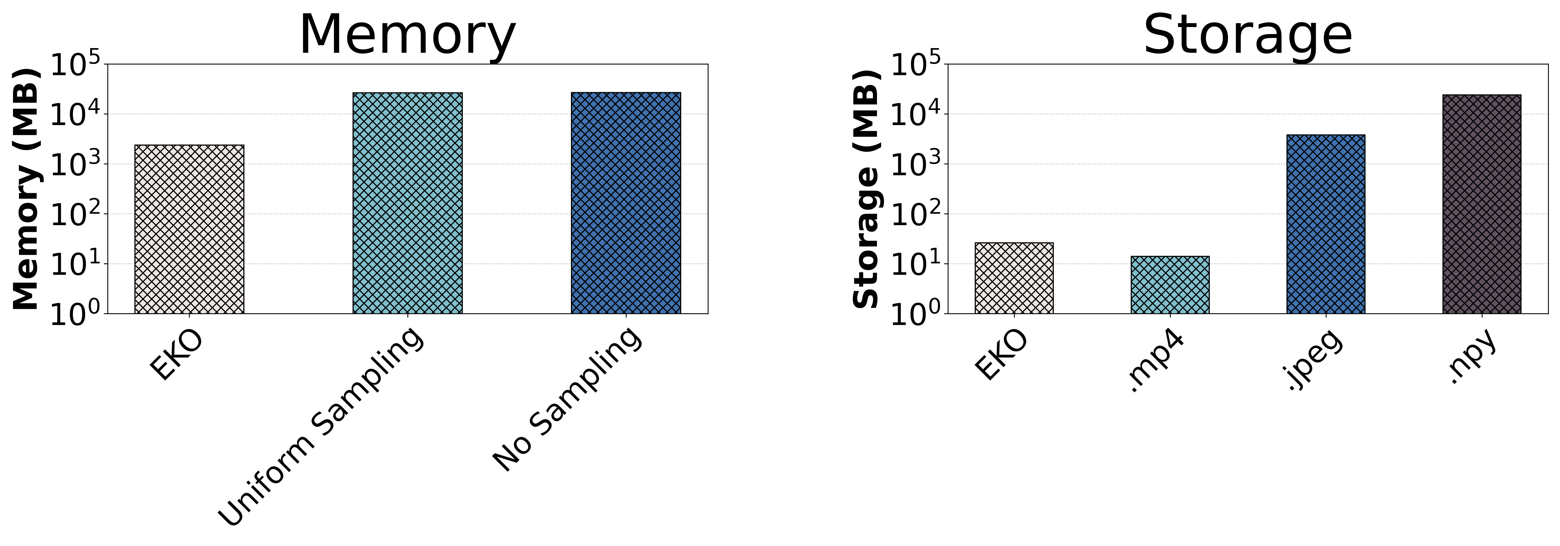
Figure 12. Memory and Storage Footprint – (a) Memory footprint of decompressed video, and (b) Storage footprint of compressed video on disk.

In this experiment, we quantify the memory and storage footprint of EKO. We focus on Q1 and configure the selectivity to 1%. We compute storage footprint based on the size of the Seattle dataset. The results are shown in Figure 12. We refer to the re-encoded video as EKO. mp4 refers to the video emitted by the $h.264$ codec. jpeg refers to storing the entire video as series of JPEG images. npy refers to the numpy representation for storing raw video content.

Impact on Memory. EKO consumes 2.37 GB of CPU memory while other algorithms consume 26 GB. This is because with the latter algorithms, the VDBMS decodes the entire video in memory. So, EKO is $~{}10\times$ memory efficient compared to Uniform and No-Sampling. The raw size of this dataset is only 240 MB. The rest of memory footprint stems from loading the SSD model. This experiment illustrates that EKO scales better to large datasets.

Impact on Storage. EKO’s re-encoded video takes 80% more space compared to mp4. The reasons are twofold. First, EKO contains more I-frames compared to the mp4 representation. Second, it generates metadata to faciliate dynamic sampling. EKO is $100\times$ and $270\times$ more space efficient compared to widely-used jpeg and npy formats, respectively.

7.7. Impact of Temporal Constraint

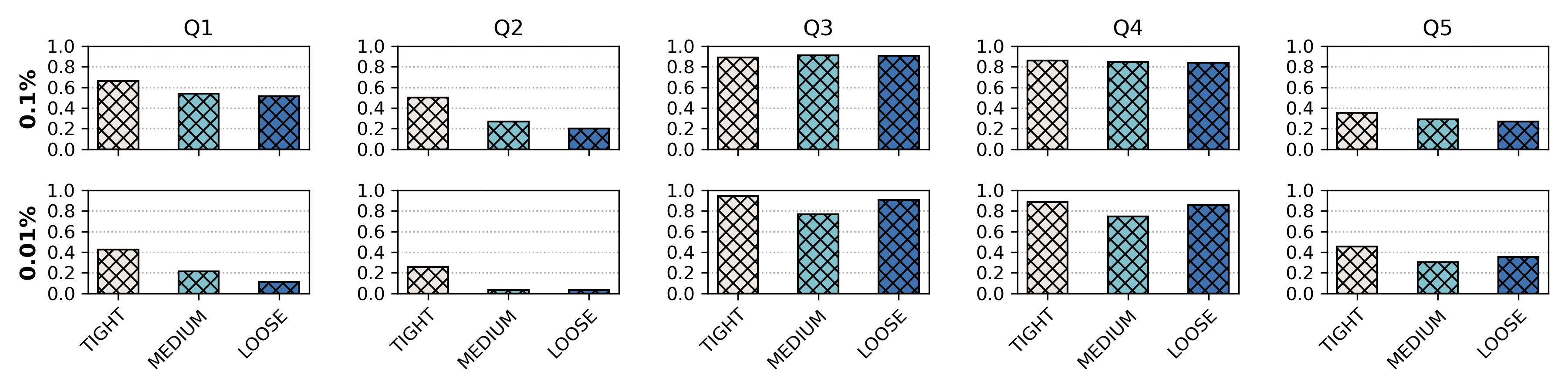
Figure 13. Impact of Temporal Constraint – Comparison of accuracy across different types of temporal constraints: (1) Tight, (2) Medium, and (3) Loose.

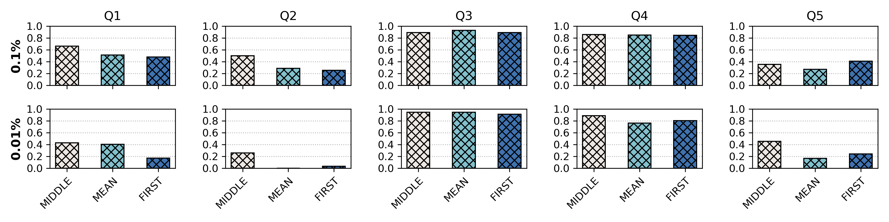
Figure 14. Impact of Frame Selection – Comparison of accuracy across different types of frame selection policies.

We next examine how the temporal constraint parameter affects the query accuracy of EKO for selectivities of 0.1% and 0.01%. We consider three configurations.

• Tight denotes a strong temporal constraint. It only allows the cluster to be formed by connecting temporally adjacent frames in the video. It is the default configuration in other experiments.

• Loose represents a much weaker temporal constraint. Clusters may be formed within a temporal span of 100 frames.

• Medium represents a configuration in between these two extremes. The clusterer may be form clusters with a temporal span ranging up to 50 frames.

The results are shown in Figure 13. The most notable observation is that relaxing the temporal constraint leads to a significant accuracy drop in many queries. With Q1 (selectivity = 0.1%), Tight outperforms Loose and Medium by 14% and 19%. With Q2, the gap increases to 48% and 65%, respectively This shows that the algorithm performs better under a tight temporal constraint. On Q3 and Q4, EKO works well under all the three constraints. This is because this query focuses on a frequent event. Since most frames satisfy the query’s constraint, the impact of the feature extractor in EKO is reduced. The importance of the temporal constraint increases when we reduce selectivity to 0.01%. When EKO must pick a smaller set of samples, it must effectively utilize the motion information present in the video.

7.8. Impact of Frame Selection

We next examine the impact of frame selection on accuracy. In this experiment, we configure EKO to use the custom feature extractor and place a Tight temporal constraint to isolate the effect of frame selection. In particular, we examine three policies for selecting frames within EKO: (1) First, (2) Mean, and (3) Middle. With First, EKO picks the first frame within each cluster while sampling frames. This is based on how I-frames are selected in canonical storage formats (avi, [n.d.]). With Mean, EKO computes the mean of all the frames within the cluster and picks the frame that is closest to the cluster’s mean frame. Lastly, Middle refers to picking the middle frame within each cluster from a temporal standpoint. We vary the selectivity from 0.1% to 0.01%. The results are shown in Figure 14.

Middle vs First. On average, Middle outperforms First by 27% across all queries. The gap between Middle and First is more prominent on queries focusing on rare events. Given the continous motion in videos, the middle frame is more representative of other frames in the cluster as opposed to the first frame. For instance, assume that the size of a given cluster is $n$ frames. The First policy leads to a maxmimal difference of $n$ frames (i.e., distance between the first and the last frames in the cluster). In contrast, the Middle policy leads to a maxmimal difference of $\frac{n}{2}$ frames. This variation in the frame selection policy is the key difference between Uniform and I-Frame in Figure 8.

Middle vs Mean. On average, Middle outperforms Mean by 26% across all queries. This is because the Mean policy does not work well with the continous motion in videos. Consider a cluster of frames wherein a car is moving from bottom left of the frame to the top right. The mean of this cluster would be a blurry smear of a car moving across the frame. While returning the frame closest to this mean frame, the Mean policy is likely to pick a non-representative frame. This experiment illustrates the importance of using the Middle policy in EKO.

8. Related Work

We now outline prior work in the areas of: (1) video analytics, (2) unsupervised image feature extraction, and (3) video storage and compression techniques.

Video Analytics. Researchers have presented several techniques for accelerating binary classification queries over videos. They are based on model cascades (Kang et al., 2017; Anderson et al., 2019), lightweight filters (Lu et al., 2018), and specialized models (Hsieh et al., 2018). NoScope (Kang et al., 2017) uses a difference detector for filtering out irrelevant frames and uses a specialized model for faster inference. TAHOMA (Anderson et al., 2019) utilizes a cascade of fast, high precision image classifiers. The lightweight models earlier in the cascade are able to quickly answer easier queries. Probabilistic Predicates (Lu et al., 2018) are lightweight models that filter out images that are not likely to satisfy the query. Instead of using high precision models as done by TAHOMA, it uses models with high recall. FOCUS uses specialized models to pre-process videos. By grouping frames with similar objects and using expensive models only for harder-to-process frames, it reduces query execution time.

Another line of research focuses on optimizing specific types of queries. BLAZEIT (Kang et al., 2018) uses control variates to optimize aggregate and limit queries by reducing the number of samples required to meet the error bound supplied by the user. MIRIS (Bastani et al., 2020) speeds up object tracking queries by varying the sampling rate based on the contents of the video. EXSAMPLE (Moll et al., 2020) illustrates the importance of picking more samples in portions of the video that are more likely to contain objects of interest.

Unsupervised Image Feature Extraction. There are several unsupervised algorithms for extracting features from images using (Xie et al., 2016; Ghasedi Dizaji et al., 2017; Caron et al., 2018). DEC uses clustering for this task (Xie et al., 2016). It updates its extraction network by jointly updating the cluster centers and the DNN parameters while minimizing the KL divergence between the data points and the desired target distribution. DEPICT (Ghasedi Dizaji et al., 2017) improves upon DEC by introducing regularization terms in the loss function for better clustering results. It also updates the network’s parameters to minimize the KL divergence between the data points and the target variable. DeepCluster (Caron et al., 2018) differs from these algorithms in that it utilizes a multi-nomial logistic loss function along with regularization.

EKO differs from prior algorithms in that it does not compute loss based on the generated cluster labels. Instead, it seeks to minimize the difference between the generated features and desired features. As discussed in § 4, this optimization is critical for videos wherein a given image may be assigned different labels based on the applied temporal constraint. Using the labels to compute the loss function would reduce the efficacy of the network.

Video Storage and Compression. Researchers have presented several systems for managing videos (Haynes et al., 2018; Daum et al., 2020; Xu et al., 2019). VSTORE periodically updates the parameters that determine how the video is stored (e.g., image quality, crop factor, resolution, sampling rate) based on the feedback from the consumers of the video. While VSTORE modifies the sampling rate across videos, it does not dynamically vary it within the video. TASM supports fast spatial, random access using a tile-based compression scheme. LIGHTDB focuses on managing virtual, augmented, and mixed reality videos. These videos consists of light fields that are higher-dimensional than traditional videos. EKO differs from these systems in that it seeks to leverage the temporal redundancy in the videos.

Prior efforts have applied deep learning for the video compression problem (Lu et al., 2019; Rippel et al., 2019; Wu et al., 2018). Specifically, one line of research focuses on minimizing distortion by maintaining as much motion information as possible compared to traditional video compression techniques (Lu et al., 2019; Wu et al., 2018). Another line of research is centered on compression networks that optimize for storage space while maintaining the same level of distortion compared to traditional compression techniques (Rippel et al., 2019). EKO differs from these efforts in that it is tailored for answering video queries. It generates more accurate results by combining adaptive sampling with the compression scheme.

9. Limitations and Future Work

EKO currently only supports binary classification queries similar to many other VDBMSs (Kang et al., 2017; Anderson et al., 2019; Lu et al., 2018; Hsieh et al., 2018). It does not support more complex queries like object localization.

⬇

SELECT target_object_bounding_boxes

FROM UA_DETRAC

WHERE vehicle_type = ’car’

AND target_vehicle_count >= 2;

We could leverage the clustering and label propagation algorithms in EKO to tackle this problem. After clustering the frames with temporal constraints, we could extend EKO to derive the movement vectors within each generated cluster during the offline, video ingestion phase. Then, during online query processing, EKO will leverage this meta-data to propagate the bounding boxes to the other frames within the cluster.

10. Conclusion

In this paper, we presented EKO, a storage engine for efficiently managing video data. EKO leverages an unsupervised sampling algorithm for picking important frames in videos. Its custom feature extractor enables it to outperform the state-of-the-art sampling algorithms with respect to accuracy on diverse queries and datasets. EKO contains a novel encoder and decoder for efficiently retrieving the key frames while processing queries. This allows the Execution Engine to fetch only the relevant frames without decoding the entire video. We show that EKO reduces query execution time by 3$\times$ and memory footprint by 10$\times$ in comparison to state-of-the-art VDBMSs.

References

- (1)
- sea ([n.d.]) [n.d.]. https://web6.seattle.gov/travelers/
- avi ([n.d.]) [n.d.]. WAVE and AVI Codec Registries. https://tools.ietf.org/html/rfc2361
- Altman (1992) Naomi S Altman. 1992. An introduction to kernel and nearest-neighbor nonparametric regression. The American Statistician 46, 3 (1992), 175–185.
- Anderson et al. (2019) Michael R Anderson, Michael Cafarella, German Ros, and Thomas F Wenisch. 2019. Physical representation-based predicate optimization for a visual analytics database. In ICDE. IEEE, 1466–1477.
- Bastani et al. (2020) Favyen Bastani, Songtao He, Arjun Balasingam, Karthik Gopalakrishnan, Mohammad Alizadeh, Hari Balakrishnan, Michael Cafarella, Tim Kraska, and Sam Madden. 2020. MIRIS: Fast Object Track Queries in Video. In SIGMOD. 1907–1921.
- Bellman (1954) Richard Bellman. 1954. The theory of dynamic programming. Technical Report. Rand corp santa monica ca.
- Caron et al. (2018) Mathilde Caron, Piotr Bojanowski, Armand Joulin, and Matthijs Douze. 2018. Deep clustering for unsupervised learning of visual features. In ECCV. 132–149.
- Chechik et al. (2010) Gal Chechik, Varun Sharma, Uri Shalit, and Samy Bengio. 2010. Large scale online learning of image similarity through ranking. (2010).
- Clement (2020) J. Clement. 2020. YouTube: hours of video uploaded every minute 2019. https://www.statista.com/statistics/259477/hours-of-video-uploaded-to-youtube-every-minute/
- Cortes and Vapnik (1995) Corinna Cortes and Vladimir Vapnik. 1995. Support-vector networks. Machine learning 20, 3 (1995), 273–297.
- Daum et al. (2020) Maureen Daum, Brandon Haynes, Dong He, Amrita Mazumdar, Magdalena Balazinska, and Alvin Cheung. 2020. TASM: A Tile-Based Storage Manager for Video Analytics. arXiv preprint arXiv:2006.02958 (2020).
- Ghasedi Dizaji et al. (2017) Kamran Ghasedi Dizaji, Amirhossein Herandi, Cheng Deng, Weidong Cai, and Heng Huang. 2017. Deep clustering via joint convolutional autoencoder embedding and relative entropy minimization. In ICCV. 5736–5745.
- Gonzalez (1985) Teofilo F Gonzalez. 1985. Clustering to minimize the maximum intercluster distance. Theoretical computer science 38 (1985), 293–306.
- Haynes et al. (2018) Brandon Haynes, Amrita Mazumdar, Magdalena Balazinska, Luis Ceze, and Alvin Cheung. 2018. Lightdb: A dbms for virtual reality video. VLDB 11, 10 (2018).
- Hsieh et al. (2018) Kevin Hsieh, Ganesh Ananthanarayanan, Peter Bodik, Shivaram Venkataraman, Paramvir Bahl, Matthai Philipose, Phillip B Gibbons, and Onur Mutlu. 2018. Focus: Querying large video datasets with low latency and low cost. In USENIX. 269–286.
- Jiang et al. (2018) Junchen Jiang, Ganesh Ananthanarayanan, Peter Bodik, Siddhartha Sen, and Ion Stoica. 2018. Chameleon: scalable adaptation of video analytics. In SIGCOMM. 253–266.
- Kang et al. (2018) Daniel Kang, Peter Bailis, and Matei Zaharia. 2018. Blazeit: Optimizing declarative aggregation and limit queries for neural network-based video analytics. arXiv preprint arXiv:1805.01046 (2018).
- Kang et al. (2017) Daniel Kang, John Emmons, Firas Abuzaid, Peter Bailis, and Matei Zaharia. 2017. Noscope: optimizing neural network queries over video at scale. arXiv preprint arXiv:1703.02529 (2017).
- Kang et al. (2020a) Daniel Kang, John Guibas, Peter Bailis, Tatsunori Hashimoto, and Matei Zaharia. 2020a. Task-agnostic Indexes for Deep Learning-based Queries over Unstructured Data. arXiv preprint arXiv:2009.04540 (2020).
- Kang et al. (2020b) Daniel Kang, Ankit Mathur, Teja Veeramacheneni, Peter Bailis, and Matei Zaharia. 2020b. Jointly optimizing preprocessing and inference for DNN-based visual analytics. arXiv preprint arXiv:2007.13005 (2020).
- Liu et al. (2016) Wei Liu, Dragomir Anguelov, Dumitru Erhan, Christian Szegedy, Scott Reed, Cheng-Yang Fu, and Alexander C Berg. 2016. Ssd: Single shot multibox detector. In ECCV. Springer, 21–37.
- Lu et al. (2019) Guo Lu, Wanli Ouyang, Dong Xu, Xiaoyun Zhang, Chunlei Cai, and Zhiyong Gao. 2019. Dvc: An end-to-end deep video compression framework. In CVPR. 11006–11015.
- Lu et al. (2018) Yao Lu, Aakanksha Chowdhery, Srikanth Kandula, and Surajit Chaudhuri. 2018. Accelerating machine learning inference with probabilistic predicates. In SIGMOD. 1493–1508.
- Moll et al. (2020) Oscar Moll, Favyen Bastani, Sam Madden, Mike Stonebraker, Vijay Gadepally, and Tim Kraska. 2020. ExSample: Efficient Searches on Video Repositories through Adaptive Sampling. arXiv preprint arXiv:2005.09141 (2020).
- Pereira et al. (2002) Fernando CN Pereira, Fernando Manuel Bernardo Pereira, Fernando C Pereira, Fernando Pereira, and Touradj Ebrahimi. 2002. The MPEG-4 book. Prentice Hall Professional.
- Redmon et al. (2016) Joseph Redmon, Santosh Divvala, Ross Girshick, and Ali Farhadi. 2016. You only look once: Unified, real-time object detection. In CVPR. 779–788.
- Rippel et al. (2019) Oren Rippel, Sanjay Nair, Carissa Lew, Steve Branson, Alexander G Anderson, and Lubomir Bourdev. 2019. Learned video compression. In CVPR. 3454–3463.
- Rosenkrantz et al. (1977) Daniel J Rosenkrantz, Richard E Stearns, and Philip M Lewis, II. 1977. An analysis of several heuristics for the traveling salesman problem. SIAM 6, 3 (1977), 563–581.
- Rousseeuw (1987) Peter J Rousseeuw. 1987. Silhouettes: a graphical aid to the interpretation and validation of cluster analysis. Journal of computational and applied mathematics 20 (1987), 53–65.
- Siegel (2019) Rachel Siegel. 2019. Tweens, teens and screens: The average time kids spend watching online videos has doubled in 4 years. https://www.washingtonpost.com/technology/2019/10/29/survey-average-time-young-people-spend-watching-videos-mostly-youtube-has-doubled-since/
- Simonyan and Zisserman (2014) Karen Simonyan and Andrew Zisserman. 2014. Very deep convolutional networks for large-scale image recognition. arXiv preprint arXiv:1409.1556 (2014).
- Suprem et al. (2020) Abhijit Suprem, Joy Arulraj, Calton Pu, and Joao Ferreira. 2020. ODIN: automated drift detection and recovery in video analytics. arXiv preprint arXiv:2009.05440 (2020).
- Tomar (2006) Suramya Tomar. 2006. Converting video formats with FFmpeg. Linux Journal 2006, 146 (2006), 10.
- VideoLAN ([n.d.]) VideoLAN. [n.d.]. x264. http://www.videolan.org/developers/x264.html
- Ward Jr (1963) Joe H Ward Jr. 1963. Hierarchical grouping to optimize an objective function. Journal of the American statistical association 58, 301 (1963), 236–244.
- Wen et al. (2020) Longyin Wen, Dawei Du, Zhaowei Cai, Zhen Lei, Ming-Ching Chang, Honggang Qi, Jongwoo Lim, Ming-Hsuan Yang, and Siwei Lyu. 2020. UA-DETRAC: A new benchmark and protocol for multi-object detection and tracking. CVIU 193 (2020), 102907.
- Wiegand et al. (2003) Thomas Wiegand, Gary J Sullivan, Gisle Bjontegaard, and Ajay Luthra. 2003. Overview of the H. 264/AVC video coding standard. TCSVT 13, 7 (2003), 560–576.
- Wu et al. (2018) Chao-Yuan Wu, Nayan Singhal, and Philipp Krahenbuhl. 2018. Video compression through image interpolation. In ECCV. 416–431.
- Xie et al. (2016) Junyuan Xie, Ross Girshick, and Ali Farhadi. 2016. Unsupervised deep embedding for clustering analysis. In ICML. 478–487.
- Xu et al. (2019) Tiantu Xu, Luis Materon Botelho, and Felix Xiaozhu Lin. 2019. Vstore: A data store for analytics on large videos. In EuroSys. 1–17.