The active centaur 2020 MK₄

Abstract

Context. Centaurs go around the Sun between the orbits of Jupiter and Neptune. Only a fraction of the known centaurs have been found to display comet-like features. Comet 29P/Schwassmann-Wachmann 1 is the most remarkable active centaur. It orbits the Sun just beyond Jupiter in a nearly circular path. Only a handful of known objects follow similar trajectories.

Aims. We present photometric observations of 2020 MK₄, a recently found centaur with an orbit not too different from that of 29P, and we perform a preliminary exploration of its dynamical evolution.

Methods. We analyzed broadband Cousins $R$ and Sloan $g^{\prime}$, $r^{\prime}$, and $i^{\prime}$ images of 2020 MK₄ acquired with the Jacobus Kapteyn Telescope and the IAC80 telescope to search for cometary-like activity and to derive its surface colors and size. Its orbital evolution was studied using direct $N$-body simulations.

Results. Centaur 2020 MK₄ is neutral-gray in color and has a faint, compact cometary-like coma. The values of its color indexes, $(g^{\prime}-r^{\prime})=0.42\pm 0.04$ and $(r^{\prime}-i^{\prime})=0.17\pm 0.04$, are similar to the solar ones. A lower limit for the absolute magnitude of the nucleus is $H_{g}=11.30\pm 0.03$ mag which, for an albedo in the range of 0.1–0.04, gives an upper limit for its size in the interval (23, 37) km. Its orbital evolution is very chaotic and 2020 MK₄ may be ejected from the Solar System during the next 200 kyr. Comet 29P experienced relatively close flybys with 2020 MK₄ in the past, sometimes when they were temporary Jovian satellites.

Conclusions. Based on the analysis of visible CCD images of 2020 MK₄, we confirm the presence of a coma of material around a central nucleus. Its surface colors place this centaur among the most extreme members of the gray group. Although the past, present, and future dynamical evolution of 2020 MK₄ resembles that of 29P, more data are required to confirm or reject a possible connection between the two objects and perhaps others.

1 Introduction

Centaurs go around the Sun following unstable paths between the orbits of Jupiter and Neptune (see for example Di Sisto & Brunini 2007; Chandler et al. 2020). While only a small fraction of the known centaurs have been found to exhibit cometary activity in the form of moderately intense eruptions, one object has managed to remain continuously active since its discovery nearly a century ago, experiencing semi-regular and comparatively very bright outbursts (see for example Jewitt 2009; Guilbert-Lepoutre 2012). This object is 29P/Schwassmann-Wachmann 1 which orbits at a distance between 5.7 AU and 6.3 AU from the Sun, beyond the region where water-ice sublimates efficiently (see for example Jewitt 2009; Guilbert-Lepoutre 2012; Wierzchos & Womack 2020). Its current orbit (see Table 1) is rather unusual among those of minor bodies located beyond Jupiter as it has both low eccentricity, $e=0.0448$, and low inclination, $i=9\aas@@fstack{\circ}39$. On June 24, 2020, J. Bulger, K. Chambers, T. Lowe, A. Schultz, and M. Willman observing with the 1.8-m Ritchey-Chretien telescope of the Pan-STARRS Project (Kaiser & Pan-STARRS Project Team 2004) from Haleakala, discovered a close orbital relative of 29P, 2020 MK₄, at an apparent magnitude $w$ of 19.8 (Drummond et al. 2020). Its latest orbit determination is shown in Table 1.

Table 1: Values of the heliocentric Keplerian orbital elements and their respective 1$\sigma$ uncertainties of comets 29P/Schwassmann-Wachmann 1, P/2008 CL94 (Lemmon), and P/2010 TO20 (LINEAR-Grauer), and centaur 2020 MK₄.

Orbital parameter		29P/Schwassmann-Wachmann 1	P/2008 CL94 (Lemmon)	P/2010 TO20 (LINEAR-Grauer)	2020 MK4
Semimajor axis, $a$ (AU)	=	5.99579143$\pm$0.00000004	6.1706$\pm$0.0002	5.6012$\pm$0.0003	6.15875$\pm$0.00007
Eccentricity, $e$	=	0.04437627$\pm$0.00000002	0.11941$\pm$0.00008	0.088533$\pm$0.000005	0.0220$\pm$0.0002
Inclination, $i$ (°)	=	9.382089$\pm$0.000002	8.34819$\pm$0.00010	2.63909$\pm$0.00012	6.66716$\pm$0.00010
Longitude of the ascending node, $\Omega$ (°)	=	312.595345$\pm$0.000011	33.4617$\pm$0.0004	43.9656$\pm$0.0008	2.344$\pm$0.002
Argument of perihelion, $\omega$ (°)	=	50.20600$\pm$0.00002	82.05$\pm$0.02	251.89$\pm$0.03	176.2$\pm$0.2
Mean anomaly, $M$ (°)	=	176.60347$\pm$0.00002	54.801$\pm$0.011	82.78$\pm$0.03	112.7$\pm$0.2
Perihelion distance, $q$ (AU)	=	5.72972056$\pm$0.00000013	5.4337$\pm$0.0004	5.1053$\pm$0.0002	6.0230$\pm$0.0010
Aphelion distance, $Q$ (AU)	=	6.26186229$\pm$0.00000004	6.9074$\pm$0.0002	6.0971$\pm$0.0003	6.29447$\pm$0.00007
Absolute magnitude, $H$ (mag)	=	8.6$\pm$1.0	8.5$\pm$0.4	5.9$\pm$0.4	11.4$\pm$0.6

The size and shape of the orbit of 2020 MK₄ are not too different from those of the orbit of 29P. Prior to the discovery of 2020 MK₄, the two closest orbital relatives of 29P (see Table 1) were the comets P/2008 CL94 (Lemmon) with a semimajor axis, $a=6.171$ AU (29P has 5.9930 AU), $e=0.1194$, and $i=8\aas@@fstack{\circ}35$ (Scotti et al. 2009; Kulyk et al. 2016; Wong et al. 2019) and P/2010 TO20 (LINEAR-Grauer) with $a=5.6006$ AU, $e=0.0887$, and $i=2\aas@@fstack{\circ}64$ (Grauer et al. 2011a; Spahr et al. 2011; Piani et al. 2011; Grauer et al. 2011b; Emel’yanenko et al. 2013; Lacerda 2013). On the other hand, the announcement MPEC of 2020 MK₄ also showed a significant increase in brightness over the course of nearly a month which could be consistent with that of an active centaur in an ourburst (Drummond et al. 2020). These two properties, an orbit similar to that of 29P and a possible rapid brightness increase, led us to investigate further. In this work, we study the nature (asteroidal versus cometary) of 2020 MK₄ using photometry and perform a preliminary exploration of its past, present, and future dynamical evolution. In Sect. 2, we describe the observations acquired and in Sect. 3, we present the results of our analysis. In Sect. 4, we explore the dynamical evolution of 2020 MK₄ and compare it with that of 29P and related objects. Our findings are discussed in Sect. 5. Finally, our conclusions are summarized in Sect. 6.

2 Observations

We obtained CCD images of 2020 MK₄ with the 0.82 m IAC80 telescope at Teide Observatory on July 16 and July 24, 2020 and also with the 1.0 m JKT telescope operated by the Southeastern Association for Research in Astronomy (SARA, Keel et al. 2017) on July 17, 2020. We used CAMELOT-2 (in Spanish, “CAmara MEjorada Ligera del Observatorio del Teide”-2) with the IAC80 telescope, a camera with an e2V 231-84 4K$\times$4K pixels CCD, a 0.336 arcsec pixel^-1 plate scale, and a 12$\aas@@fstack{\prime}$3$\times$12$\aas@@fstack{\prime}$3 effective field of view. With the JKT, we used a 2K$\times$2K pixels ANDOR Ikon-L 2048 CCD camera with a 0.34 arcsec pixel^-1 plate scale and a 11$\aas@@fstack{\prime}$6$\times$11$\aas@@fstack{\prime}$6 field of view.

On July 16 and with the IAC80, we obtained a series of images (exposure times of 120 s each) using the Cousins R filter between 1:04 and 2:19 UT. On July 17 and with the JKT, we obtained a series of 93 images (exposure times of 90 s each) using the Sloan r’ filter between 0:13 and 2:37 UT. Finally, between July 23, 23:01 UT and July 24, 00:54 UT, with the IAC80, we obtained a series of images (exposure times of 300 s each) using the Sloan g’, r’, and i’ filters (12 images in the r’, four in the g’, and four in the i’-band, doing four series of r’, g’, r’, i’, r’ images). We used sidereal tracking and the individual exposure time — in particular the first two nights — was selected to ensure that the movement of the comet was smaller than the value of the seeing to avoid traces. Images were bias and flat-field corrected (using sky flats). Observational circumstances are summarized in Table 2. On July 24, we also observed the Landolt standard field star Mark A (Landolt 1992) to derive an absolute photometric calibration.

Table 2: Circumstances of observation of centaur 2020 MK₄.

Date	Tel.	UT-range	X	$r_{h}$	$\Delta$	$\alpha$	$\theta_{\sun}$	$\theta_{-V}$	Filters
		(h:m)		(AU)	(AU)	(°)	(°)	(°)
July 16	IAC80	01:04 – 02:19	1.80 – 1.85	6.228	5.220	1.3	322.5	255.3	R
July 17	JKT	00:13 – 02:37	1.80 – 1.96	6.228	5.220	1.2	329.8	255.3	r’
July 23/24	IAC80	23.01 – 00:54	1.80 – 2.15	6.229	5.223	1.4	23.2	255.7	g’, r’, i’

3 Results

3.1 Cometary-like activity

During the analysis of the images of 2020 MK₄, we immediately noticed that the full width at half maximum (FWHM) of the point spread function (PSF) of 2020 MK₄ was systematically wider than that of the stars during the first two nights of observations, suggesting the presence of a faint, compact cometary-like coma. In order to determine if the object was active, we made a direct comparison of its surface brightness profile with the profiles of the stars in the field. We applied the following steps. First, we aligned the images so that the stars were all lined up and stacked onto one another. A set of bright stars in the combined image was selected and, for these stars, the intensity versus distance to centroid was extracted, normalized to the maximum, and combined to retrieve a high signal-to-noise ratio (S/N) stellar profile. In a second step, all the images were realigned, so then 2020 MK₄ was lined up and then combined (see Fig. 1). The profile of the object was subsequently extracted from the combined image and normalized. Finally, the resulting stellar profile and that of the object were fitted with a Moffat function and plotted together to compare them. In Fig. 2, we show the analysis of the profile of the combined images obtained on July 16 and 17. During both nights, the brightness profile of 2020 MK₄ was significantly wider, indicating that 2020 MK₄ had a coma.

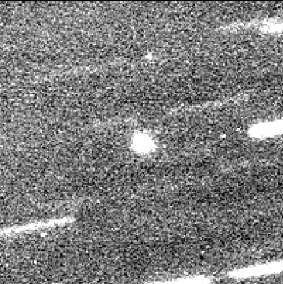
Figure 1: Observations of 2020 MK₄. Left panel: Image of 2020 MK₄ obtained on July 17, 2020 with the JKT telescope. This image is a combination of 93 images (exposure time of 90 s each), realigned so 2020 MK₄ was lined up. The field is 68″$\times$68″; north is up, and east is to the left. Right panel: Image combined on the comet minus the same combination of images centered on a bright star. Both images were sky subtracted and normalized to the peak before subtraction. It is important to notice that there is a circular residual compatible with the presence of a compact faint coma around 2020 MK₄. In this case, the field of view is 34″$\times$34″. The coma has a diameter of about 4$\aas@@fstack{\prime\prime}$1 or 15 500 km at the geocentric distance indicated in Table 2.

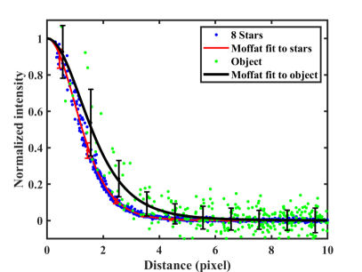
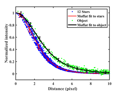
Figure 2: Profile analysis of the combined images of 2020 MK₄ obtained on July 16 (left panel) and July 17 (right panel). Each plot contains the values of the normalized intensity as a function of the distance from the centroid (in pixels) for the stars (blue dots), the Moffat fit for the stars (red line), values of normalized intensity for the object (green dots), and the Moffat fit for the object (black line). Red bars correspond to the stars while black bars correspond to the object, and they are placed in the middle of the interval; an artificial offset in the x-axis was introduced to avoid overlapping symbols. It is important to notice that the profile of 2020 MK₄ is significantly wider both nights, confirming that 2020 MK₄ shows clear signs of cometary-like activity.

We also used the image with a higher S/N obtained on July 17 to check if the difference between the object and star profile could be due to the proper motion of the object. In an attempt to see the coma, we subtracted the image of a bright star from the combined image in which the stars were aligned from that of 2020 MK₄ in the combined image for which 2020 MK₄ was lined up. In order to do that, we subtracted the sky value and normalized the images to the brightness peak of the object and star profile, respectively, carefully aligning the object and star, and we subtracted the star image. The result of this procedure is shown in Fig. 1. The resulting image presents an almost perfectly circular, but doughnut-shaped residual. This corresponds to the expected shape of a compact coma and not to the effect of the proper motion of the object that would produce residuals only in the direction of the motion. Therefore, we conclude that 2020 MK₄ was active at the time of the observations.

3.2 Photometry and colors

In order to derive a limit for the absolute magnitude and obtain the colors of the object, we did aperture photometry of the combined images for each night using standard tasks in the Image Reduction and Analysis Facility (IRAF). We followed a procedure similar to the one described in Licandro et al. (2019). We used an aperture diameter equivalent to the object’s FWHM. We obtained the absolute calibration using field stars with Sloan g’, r’, and i’ magnitudes determined in the Pan-STARRS catalogue and, on July 24, also using the flux calibrated Landolt stars in the field of the star Mark A and the transformation equations from Bilir et al. (2005) and Rodgers et al. (2006) when needed. We obtained a magnitude of $r^{\prime}=18.73\pm 0.07$, $r^{\prime}=18.88\pm 0.03$, and $r^{\prime}=18.84\pm 0.03$ on July 16, 17, and 24, respectively, and the colors $(g^{\prime}-r^{\prime})=0.42\pm 0.04$ and $(r^{\prime}-i^{\prime})=0.17\pm 0.04$ on July 24.

Using Eq. (1) from Jewitt & Luu (2019), we derived a lower limit for the absolute magnitude of 2020 MK₄, $H_{g}=11.30\pm 0.03$ mag. Assuming a value of the visible geometric albedo between 0.1 and 0.04, this value of $H_{g}$ provides an upper limit for the radius of the nucleus of the object, $R_{\rm N}$, between 23 km and 37 km. Using this value of $H_{g}$ and assuming that this is the real absolute magnitude of the centaur, the apparent magnitude of 2020 MK₄ during June 2020 could have been $19.0$ mag$<r^{\prime}<18.8$ mag. However, the observed brightness reported by Pan-STARRS in Drummond et al. (2020) shows that the object was 1 or 2 magnitudes fainter, with values around 21 mag (in $w$) early in June and 19.9 mag at the end of the month, indicative of an activation around early June or perhaps earlier than that.

In order to make an approximate evaluation of the relative contribution of the nucleus to the total flux in the used aperture, we subtracted a bright field star of known r’ magnitude from the comet images as we did above. In this case, we first scaled the star to $r^{\prime}$=20.73, 19.73, and 19.53 magnitude (in other words, 2.0, 1.0, and 0.8 magnitudes fainter than that of the comet). The normalized radial profiles of the resulting images are shown in Fig. 3 together with the profile of a simulated isotropic coma (thick, black curve). The profile of an isotropic coma was generated using the mkobject task of IRAF, a $1/\rho$ profile for the coma, and a Moffat profile with the same parameters obtained from the field stars to simulate the seeing. Figure 3 suggests that the nuclear magnitude is $\sim$0.8–1.0 mag fainter than the limit we obtained, that is $H_{g}\sim 12.30$ mag, and thus the nucleus contributes about 66% to 52% of the total flux in the used aperture. If the nucleus is brighter than 19.53 mag, then a “hole” in the comet’s profile should appear at the center; if it is fainter, then the coma profile should be much more compact than the isotropic assumption. Our results suggest a value of $R_{\rm N}$ between 15 km and 23 km.

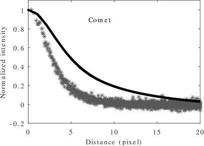
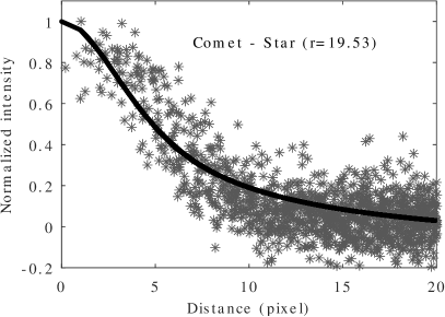
Figure 3: Evaluating the coma of 2020 MK₄. Normalized radial profile of the combined images of 2020 MK₄ obtained on July 17 minus a star profile of a different brightness (the assumed nucleus) together with the normalized radial profile of an isotropic coma (thick, black curve, see text). Upper-left panel: The profile of the comet. Upper-right panel: The profile of the comet minus that of a nucleus (a star) of $r^{\prime}$=20.73 mag. Bottom-left panel: The profile of the comet minus that of a nucleus of $r^{\prime}$=19.73 mag. Bottom-right panel: The profile of the comet minus that of a nucleus of $r^{\prime}$=19.53 mag. It is important to notice that the coma that remains once a nucleus of $r^{\prime}$=19.53 mag has been subtracted resembles what an isotropic coma should look like.

On the other hand, we noticed that the colors of 2020 MK₄ are similar to the solar ones. The colors of 2020 MK₄ correspond to those of the members of the group of the gray centaurs (see Peixinho et al. 2003; Tegler et al. 2003, 2008, 2016); in fact, it is perhaps one of the less red centaurs discovered thus far. It is well known that centaur objects exhibit a peculiar physical property and that their visual colors divide the population into two distinct groups: gray and red centaurs. The colors of 2020 MK₄ are also consistent with those observed in other active centaurs; they all belong to the gray population, with the exception of (523676) 2013 UL₁₀, a red centaur (Mazzotta Epifani et al. 2018). Melita & Licandro (2012) showed that the different thermal reprocessing on the surface of bodies of the red group on one side and the active and gray groups on the other is responsible for the observed bimodality in the distribution of the surface colors of the centaurs; the color distribution of the gray centaurs is similar to that of comet nuclei because gray centaurs likely had cometary activity. As we discussed above, the flux in the used aperture is not just due to the brightness of the nucleus, but to the nucleus plus the dust coma. The coma can contribute with $\sim$50% of the total flux and this can also have some effect on the measured color. In any case and in order to blue a red centaur so that it almost has a neutral color, the intrinsic color of the coma should be unusually blue. However, it is clear that once its active nature has been confirmed, further observations with a higher S/N are needed to understand the behavior of this centaur better.

4 Context and orbital evolution

Centaur 2020 MK₄ has been confirmed as active, but we still have a question regarding the similarity between its orbit and that of comet 29P/Schwassmann-Wachmann 1 and related objects (see Table 1). The characterization of its orbital context requires the study of the present-day orbital architecture of the sample of known objects that populate this region of the orbital parameter space. Here, such a study is carried out by exploring the distributions of mutual nodal distances and orientations in space. In order to analyze the results, we produced histograms using the Matplotlib library (Hunter 2007) with sets of bins computed using NumPy (van der Walt et al. 2011; Harris et al. 2020) by applying the Freedman and Diaconis rule (Freedman & Diaconis 1981); kernel density estimations were carried out using the Python library SciPy (Virtanen et al. 2020).

On the other hand, the assessment of the past, present, and future orbital evolution of 2020 MK₄ should be based on the statistical analysis of results from a representative sample of $N$-body simulations. Here, such calculations were carried out using a direct $N$-body code implemented by Aarseth (2003) that is publicly available from the website of the Institute of Astronomy of the University of Cambridge. This software uses the Hermite integration scheme described by Makino (1991). Results from this code compare well with those from Laskar et al. (2011) among others, as extensively discussed by de la Fuente Marcos & de la Fuente Marcos (2012).

The initial conditions used in our calculations come from the orbit determination in Table 1 which has been released by Jet Propulsion Laboratory’s Solar System Dynamics Group Small-Body Database (JPL’s SSDG SBDB). Input data used in our orbital context analysis and in our simulations were obtained from JPL’s HORIZONS online solar system data and ephemeris computation service (Giorgini 2011, 2015). Most data were retrieved from JPL’s SBDB and HORIZONS using tools provided by the Python package Astroquery (Ginsburg et al. 2019). Although the orbit determination still needs to be improved (the orbital size and shape are relatively good, but the orientation in space is still somewhat uncertain), particularly when compared with that of 29P in Table 1, we believe that it is good enough to reach some robust conclusions given the nature of our calculations. In addition to studying some representative orbits, we performed longer calculations that applied the Monte Carlo using the Covariance Matrix (MCCM) methodology described by de la Fuente Marcos & de la Fuente Marcos (2015) in which a Monte Carlo process generates control or clone orbits (3000) based on the nominal orbit, but adding random noise on each orbital element by making use of the covariance matrix, which was also retrieved from JPL’s SSDG SBDB.

4.1 Orbital context

Here, we focus on the sample of objects with $a\in(5.4,7)$ AU, $e<0.15$, and $i<10$° that includes the four objects in Table 1 and eight other known small bodies that follow this type of low-eccentricity, low-inclination orbit located just beyond that of Jupiter: 2011 FS₅₃, 2012 BS₇₆, 2014 EB₁₃₂, 2014 EF₁₁₅, 2014 EM₁₂₀, 2014 EO₆₈, 2014 EW₇₇, and 2016 AK₅₁. Unfortunately, all of them have very poor orbit determinations based on about a dozen observations and spanning data arcs of 2 to 18 days. The distribution of mutual nodal distances (their absolute values) was computed as described in Appendix A, using data from JPL’s SSDG SBDB. A small mutual nodal distance implies that the objects might experience close flybys, but this must be confirmed by using $N$-body simulations.

Our sample produced 66 pairs of mutual nodal distances, ${\Delta}_{\pm}$ (the results for each pair come from a set of 10⁴ pairs of virtual objects as described in Appendix A). The distribution of mutual nodal distances for the ascending mutual nodes is shown in the upper panel of Fig. 4 and the one corresponding to the descending mutual nodes is displayed in the bottom panel of Fig. 4. These distributions were computed using mean values and uncertainties in the orbit determinations as described in Appendix A. The first percentile of the distribution in ${\Delta}_{+}$ is equal to 0.22 AU and the one of ${\Delta}_{-}$ is 0.04 AU. The first percentile is often considered as the statistically significant boundary to select severe outliers.

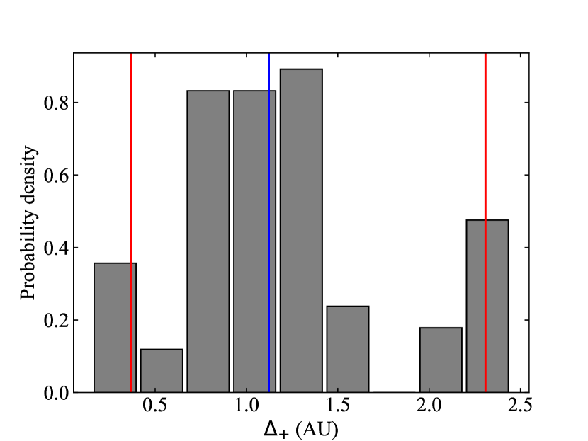
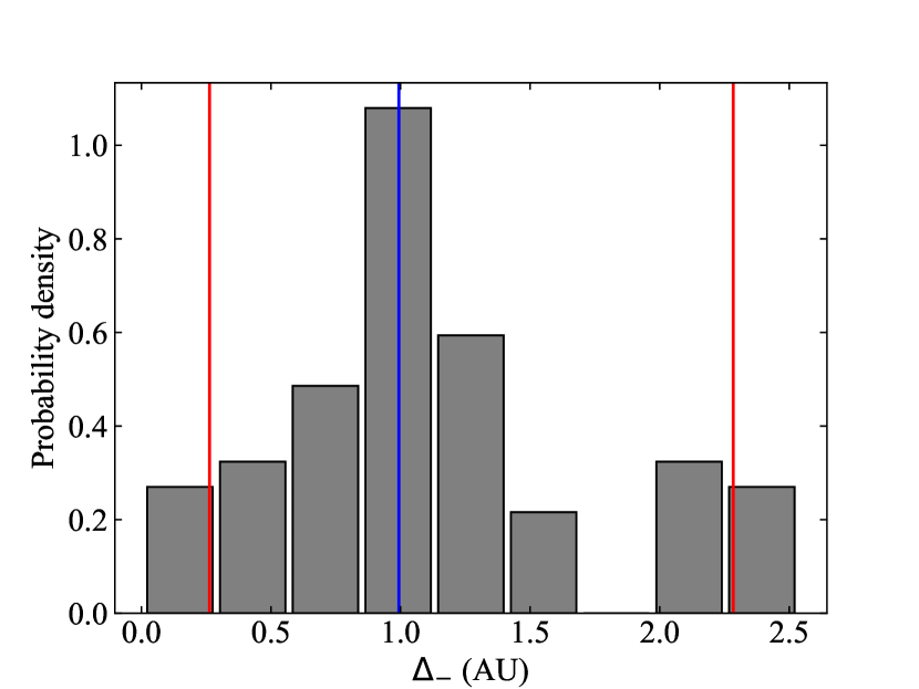
Figure 4: Distribution of mutual nodal distances. Upper panel: For the ascending mutual nodes of the sample of 12 small bodies following orbits similar to that of 29P. The median is shown in blue and the 5th and 95th percentiles are in red. Bottom panel: For the descending mutual nodes of the same sample. In the histogram, we use bins computed using the Freedman and Diaconis rule (Freedman & Diaconis 1981) and counts to form a probability density so the area under the histogram will sum to one.

When considering the 66 pairs of mutual nodal distances, two clear outliers emerge: For 29P and 2020 MK₄ ${\Delta}_{+}=0.1536\pm 0.0005$ AU (median, and the 16th and 84th percentiles) and for 29P and P/2010 TO20 (LINEAR-Grauer) ${\Delta}_{-}=0.0083\pm 0.0003$ AU. In both cases, it is statistically unlikely that the small values of the mutual nodal distances could be accidental (see Fig. 5) and some type of connection must exist, be it in the form of resonant forces or a true physical relationship in which both objects come from a disrupted parent body. If disruption events are the cause of the small mutual nodal distances, two of them may be required to explain the observed values. The distributions of angular distances between pairs of orbital poles and perihelia were computed as described in Appendix B using data from JPL’s SSDG SBDB. The orientations in space of the orbits of these objects are compatible with those coming from a continuous uniform distribution (average and standard deviation values, see Fig. 6, upper panel) of angular distances between pairs of orbital poles and perihelia.

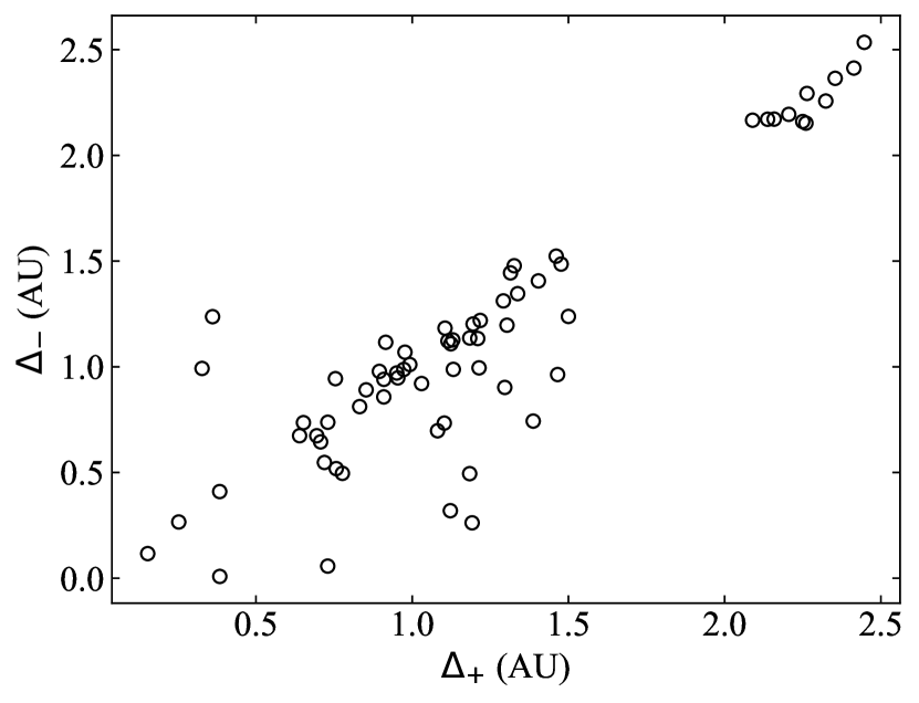
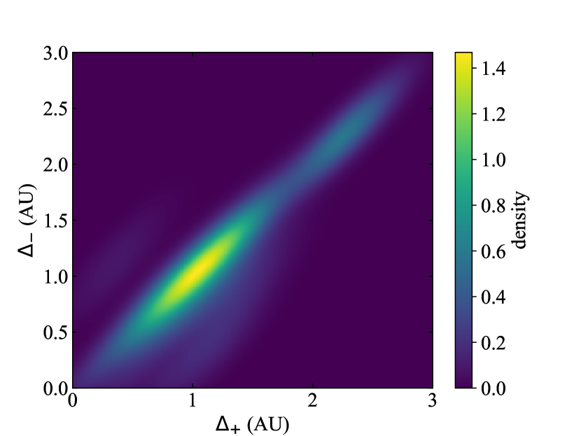
Figure 5: Mutual nodal distances of objects in 29P-like orbits. Upper panel: 66 pairs of mutual nodal distances. Bottom panel: Gaussian kernel density estimation of the same data.

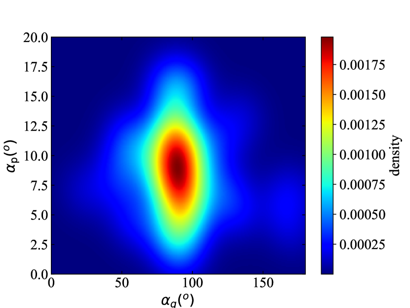
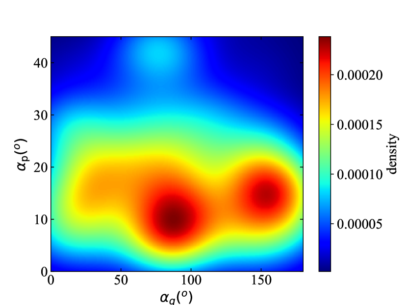
Figure 6: Orientations in space of the orbits. Upper panel: Gaussian kernel density estimation for the 66 pairs of 29P-like orbits. Bottom panel: Gaussian kernel density estimation for the 171 pairs of NC orbits.

It may be argued that our choice of parameter boundaries to select the sample of minor bodies that follow 29P-like orbits is somewhat artificial. Roberts & Muñoz-Gutiérrez (2021) have studied the dynamics of small bodies that go around the Sun between the orbits of Jupiter and Saturn. In their work, it is argued that all of these bodies have orbits similar to that of comet 29P. They call this group the “near centaurs” or NCs that have values of the perihelion distance $q>5.204$ AU and the aphelion distance $Q\in(5.6,9.583)$ AU. JPL’s SSDG SBDB shows that this group includes 42 objects; after discarding all the fragments of comet D/1993 F2 (Shoemaker-Levy 9), and 2004 VP₁₁₂ and 2007 TB₄₃₄ because their orbit determinations are very uncertain, our working sample includes 19 objects. This NC sample does not include P/2010 TO20 (LINEAR-Grauer) nor most of the objects in our previous sample with the exception of 2011 FS₅₃, because their perihelia are shorter, but it does include the other three objects in Table 1.

If we repeat the previous analysis for these NCs, we obtain Figs. 7 and 8. For this sample, the first percentile of the distribution in ${\Delta}_{+}$ is equal to 0.015 AU and the one of ${\Delta}_{-}$ is 0.040 AU. When considering the 171 pairs of mutual nodal distances (see Fig. 8), four clear outliers emerge: For 29P and (494219) 2016 LN₈ ${\Delta}_{-}=0.003090\pm 0.000002$ AU, for 2015 UH₆₇ and P/2005 T3 (Read) ${\Delta}_{-}=0.03\pm 0.02$ AU, for P/2008 CL94 (Lemmon) and P/2011 C2 (Gibbs) ${\Delta}_{+}=0.0096\pm 0.0005$ AU, and for P/2008 CL94 (Lemmon) and P/2015 M2 (PANSTARRS) ${\Delta}_{+}=0.0047\pm 0.0004$ AU. Although Roberts & Muñoz-Gutiérrez (2021) argue that most of these objects are partly subjected to various mean-motion resonances with the giant planets, such small values of ${\Delta}_{\pm}$ are suggestive of an interacting population in which fragmentation events may be taking place during outburst episodes.

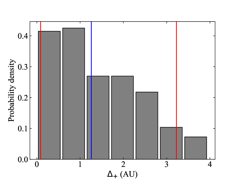
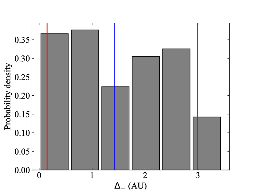
Figure 7: Distribution of mutual nodal distances. Upper panel: For the ascending mutual nodes of the sample of 19 NCs. The median is shown in blue and the 5th and 95th percentiles are in red. Bottom panel: For the descending mutual nodes of the same sample. In the histogram, we use bins computed using the Freedman and Diaconis rule (Freedman & Diaconis 1981) and counts to form a probability density so the area under the histogram will sum to one.

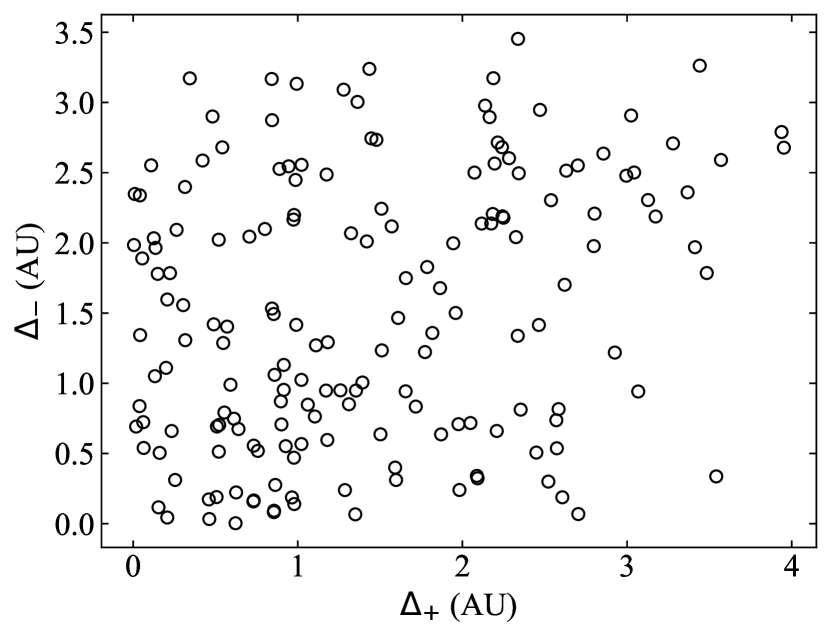
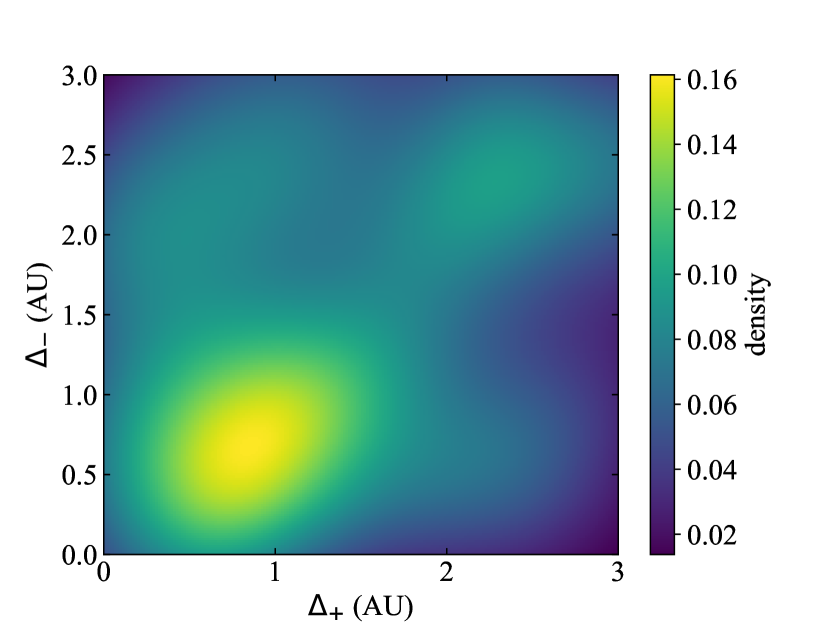
Figure 8: Mutual nodal distances of NCs. Upper panel: 171 pairs of mutual nodal distances. Bottom panel: Gaussian kernel density estimation of the same data.

Additional evidence along this line of reasoning comes from the study of the distributions of angular distances between pairs of orbital poles and perihelia defined by the angles $\alpha_{\rm p}$ and $\alpha_{q}$ (computed as described in Appendix B, see Fig. 6, bottom panel), and the difference in time of perihelion passage, $\Delta{T_{q}}$. The first percentiles of these distributions are 2$\aas@@fstack{\circ}$68, 5$\aas@@fstack{\circ}$64, and 0.062 yr, respectively. Outlier pairs are as follows: 2013 SO₁₀₇ and 2014 HY₁₉₅ with $\alpha_{\rm p}=2\aas@@fstack{\circ}252\pm 0\aas@@fstack{\circ}003$, 39P/Oterma and P/2005 S2 (Skiff) with $\alpha_{q}=5\aas@@fstack{\circ}51\pm 0\aas@@fstack{\circ}12$, 39P/Oterma and P/2005 T3 (Read) $\alpha_{q}=1\aas@@fstack{\circ}2_{-0\aas@@fstack{\circ}3}^{+0\aas@@fstack{\circ}5}$, P/2005 T3 (Read) and P/2008 CL94 (Lemmon) with $\alpha_{\rm p}=2\aas@@fstack{\circ}236\pm 0\aas@@fstack{\circ}011$, 2015 UH₆₇ and 2020 MK₄ with $\Delta{T_{q}}=0.013_{-0.008}^{+0.010}$ yr, and 2020 MK₄ and P/2015 M2 (PANSTARRS) with $\Delta{T_{q}}=0.053\pm 0.010$ yr. Some of these objects have highly correlated orbits in terms of their orientation in space and timing, which are difficult to explain by chance or mean-motion resonances alone.

4.2 Current dynamical status

Minor body 2020 MK₄ goes around the Sun between the orbits of Jupiter and Neptune, so it is a centaur. It has a current value of the Tisserand’s parameter, $T_{\rm J}$ (Murray & Dermott 1999), of 3.005; therefore, and following Levison & Duncan (1997), it cannot be a Jupiter-family comet because the value is not in the interval (2, 3), even if we account for the uncertainties. In contrast, 29P has a value of the Tisserand parameter of 2.984 and it has remained consistently under 3.0 since its discovery back in 1927. In this context, the Tisserand parameter, which is a quasi-invariant, is given by the expression:

$$T_{\rm J}=\frac{a}{a_{\rm J}}+2\ \cos{i}\ \sqrt{\frac{a_{\rm J}}{a}\ (1-e^{2})}\,,$$ (1)

where $a$, $e$, and $i$ are the semimajor axis, eccentricity, and inclination of the orbit of the minor body under study, respectively, and $a_{\rm J}$ is the semimajor axis of the orbit of Jupiter (Murray & Dermott 1999). The functional form of this parameter makes it robust against relatively large variations in the values of the relevant orbital parameters, which helps its application to objects with rather chaotic orbital evolutions.

The panels on the right-hand side of Figure 9 show the short-term evolution of relevant parameters of representative control orbits with Cartesian vectors separated by $\pm$3$\sigma$ and $\pm$9$\sigma$ from the nominal values in Table 3. The orbital evolution is very chaotic and some instances lead to ejections integrating into the past (not shown) and towards the future. Ejections are the result of very close encounters with Jupiter and other giant planets, but also with the Sun following episodes similar to those described in de la Fuente Marcos et al. (2015) for comet 96P/Machholz 1. Close encounters with Jupiter drive the very chaotic short-term behavior observed in the panels on the left in Fig. 9. The evolution of $T_{\rm J}$ (bottom panels) shows that 2020 MK₄ is unlikely to become a long-term member of the Jupiter-family comet dynamical class for control orbits in the $\pm$3$\sigma$ range, both in the past and the future. However, control orbits more separated from the nominal one, $\pm$9$\sigma$, show extended lengthy incursions inside the Jupiter-family comet orbital domain (the value of $T_{\rm J}$ librates, see bottom panels in Fig. 9). The bottom panel of Figure 10 shows that 29P has a much lower probability of being a long-term member of the Jupiter-family comet group (the control orbits are based on the data in Table 4). In general terms, the orbital evolution displayed in Figs. 9 and 10 is similar and nearly equally chaotic (readers are encouraged to compare the evolution of $a$, $e$, and $i$ in both figures); this is the standard dynamical behavior for objects in these orbits (see for example Grazier et al. 2019).

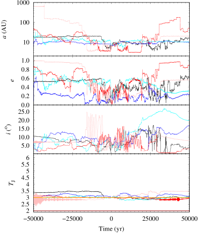
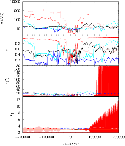
Figure 9: Short-term evolution of relevant parameters of 2020 MK₄. Left panels: focus on a shorter time window but correspond to the same data shown in the right-hand side panels. Right panels: evolution of the semimajor axis, $a$ (upper panels), of the nominal orbit (in black) as described by the orbit determination in Table 1 and those of control orbits or clones with Cartesian vectors separated $+$3$\sigma$ (in blue), $-$3$\sigma$ (in cyan), $+$9$\sigma$ (in red), and $-$9$\sigma$ (in pink) from the nominal values in Table 3. The second from the top panels show the evolution of the eccentricity, $e$, for the same sample of control orbits. The second from the bottom panels display the inclination, $i$. The bottom panels show the variations of the Tisserand’s parameter, $T_{\rm J}$ and include the boundary references 2 (in brown) and 3 (in orange). The output time-step size is 20 yr, the origin of time is epoch 2459000.5 TDB.

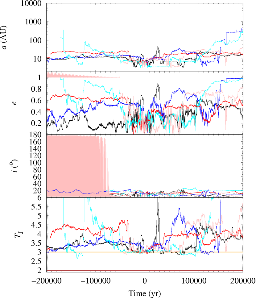
Figure 10: Short-term evolution of relevant parameters of comet 29P/Schwassmann-Wachmann 1. Similar to Fig. 9 but for data in Table 4. The output time-step size is 20 yr, the origin of time is epoch 2459000.5 TDB.

Figure 11 shows the shorter-term evolution of relevant parameters of representative orbits for all the objects in Table 1. Both 29P and 2020 MK₄ are not currently experiencing very close encounters with Jupiter and Saturn, but P/2008 CL94 (Lemmon) approaches Jupiter inside the Hill radius of the planet and P/2010 TO20 (LINEAR-Grauer) does the same for both Jupiter and Saturn.

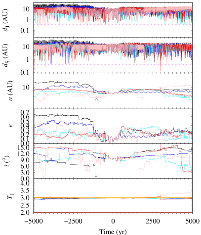
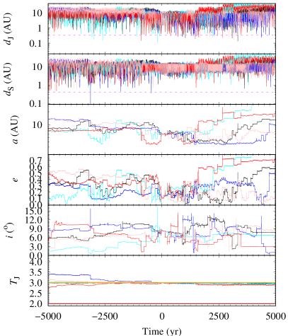
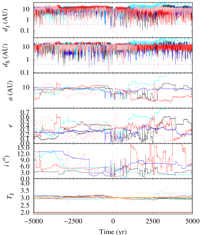
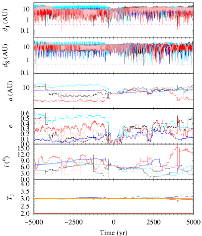
Figure 11: Short-term evolution of relevant parameters of comets 29P/Schwassmann-Wachmann 1, P/2008 CL94 (Lemmon), and P/2010 TO20 (LINEAR-Grauer), and centaur 2020 MK₄. Results for 29P are shown in the upper left panels, those of P/2008 CL94 are displayed in the upper right panels, the bottom left panels show those of P/2010 TO20, and the bottom right panels focus on 2020 MK₄. For each set of panels, we show the evolution of the distances to Jupiter (top panel) and Saturn (second to top) of the nominal orbit (in black) as described by the corresponding orbit determination in Table 1 and those of control orbits or clones with Cartesian vectors separated $+$3$\sigma$ (in blue), $-$3$\sigma$ (in cyan), $+$9$\sigma$ (in red), and $-$9$\sigma$ (in pink) from the nominal values in Appendix C. The Hill radii of Jupiter, 0.338 AU, and Saturn, 0.412 AU, is shown in red. The third panel from the top shows the evolution of the semimajor axis, $a$. The third panel from the bottom shows the evolution of the eccentricity, $e$, for the same sample of control orbits. The second panel from the bottom displays the inclination, $i$. The bottom panel shows the variations in Tisserand’s parameter, $T_{\rm J}$, and includes the boundary references 2 (in brown) and 3 (in orange). The output time-step size is 1 yr, and the origin of time is epoch 2459000.5 TDB.

4.3 Future orbital evolution

Figure 9 shows that 2020 MK₄ is not unlikely to leave the Solar System within the next 200 kyr. However, close encounters with Jupiter may lead to an eventual collision with the giant planet. A similar picture, but less extreme, emerges for 29P when considering Fig. 10 and is consistent with the previous work by Neslušan et al. (2017), Sarid et al. (2019), and Roberts & Muñoz-Gutiérrez (2021). Longer calculations carried out using MCCM to generate control orbits of 2020 MK₄ (see Fig. 12, right-hand side panel) yield a value for the probability of ejection from the Solar System during the next 0.5 Myr of 0.48$\pm$0.03 (average and standard deviation). These results are robust as they remain consistent between orbit determinations.

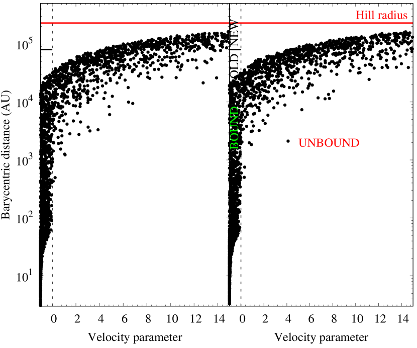
Figure 12: Past and future of 2020 MK₄. Values of the barycentric distance as a function of the velocity parameter 0.5 Myr into the past (left panel) and future (right panel) for 3000 control orbits of 2020 MK₄. The velocity parameter is the difference between the barycentric and escape velocities at the computed barycentric distance in units of the escape velocity. Positive values of the velocity parameter identify control orbits that could be the result of capture (left panel) or lead to escape (right panel). The thick black line corresponds to the aphelion distance —$a\ (1+e)$, limiting case $e=1$— that defines the domain of dynamically old comets with $a^{-1}>2.5\times 10^{-5}$ AU^-1 (see Królikowska & Dybczyński 2017); the thick red line marks the radius of the Hill sphere of the Solar System (see for example Chebotarev 1965).

The bottom right panels of Figure 11 show that the future evolution of 2020 MK₄ becomes more chaotic a few hundred years into the future when it will start experiencing close encounters under the Hill radius with Jupiter. Nearly 700 yr into the future, it will start experiencing close encounters under the Hill radius with Saturn as well and the overall orbital evolution will become even more chaotic. A similar behavior is observed for 29P (see Fig. 11, upper left panels). P/2008 CL94 is far more engaged with Jupiter, interacting at a close range now and in the future, but it will remain fairly detached from Saturn (see Fig. 11, upper right panels). P/2010 TO20 remains strongly perturbed by Jupiter and is slightly less affected by Saturn (see Fig. 11, bottom left panels), although close encounters with both planets seem to drive its very chaotic orbital evolution. All these objects have a significant probability of leaving the Solar System in the relatively near future.

4.4 Past orbital evolution: Possible origin

The key unknowns to determine are the origin of 2020 MK4 and whether 2020 MK4 and 29P, and perhaps other objects, are related. Figures 9 and 10 show that there is a clear resemblance between the past orbital evolution of both objects, but this does not imply a physical relationship as the evolutions are both very chaotic. An exploration of this scenario requires the analysis of a large set of $N$-body simulations integrating backwards in time for this pair. The statistical study of minimum approach distances may help in supporting or rejecting a scenario in which 2020 MK₄ could be a fragment of 29P.

Using a sample of 20 000 pairs of Gaussianly distributed control orbits based on the Cartesian vectors in Tables 3 and 4 and integrated backwards in time for 5 000 yr (a similar sample integrated for 10 000 yr produces nearly the same results), we have studied how the distribution is for minimum approach distances and also the relative position of Jupiter during such close encounters. The top panel of Figure 13 shows the distribution; the median and the 16th and 84th percentiles of the minimum approach distance distribution are $0.27_{-0.15}^{+0.21}$ AU. Our calculations show that close encounters between these objects under one Lunar distance are possible (the closest flyby was at about 363 000 km), but the most surprising result is that the probability of this pair experiencing a close encounter (following the distribution in Fig. 13, top panel) while 2020 MK₄ has a negative Jovicentric energy is 2.7% and most of these temporary captures were within 100 Jovian radii. About 63% of close encounters take place within 1 Hill radius of Jupiter. The distribution of the durations of many of these capture events is shown in Fig. 14 (top panel and second panel from the top). Comet 29P tends to experience slightly longer captures than 2020 MK₄.

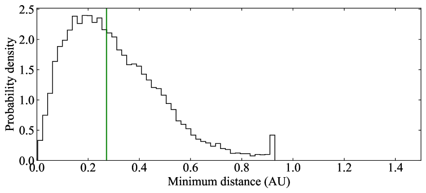
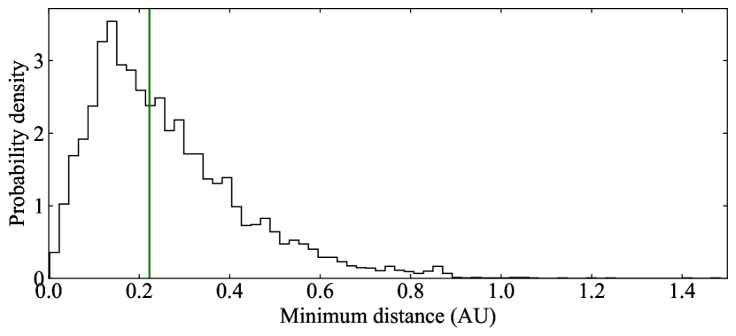
Figure 13: Distribution of minimum approach distances. Upper panel: For the pair 29P/Schwassmann-Wachmann 1 and 2020 MK₄. Middle panel: For the pair P/2008 CL94 (Lemmon) and 2020 MK₄. Bottom panel: For the pair P/2010 TO20 (LINEAR-Grauer) and 2020 MK₄. Median values are displayed as vertical green lines. The bins were computed using the Freedman and Diaconis rule implemented in NumPy (van der Walt et al. 2011; Harris et al. 2020). In the histogram, we use counts to form a probability density so the area under the histogram will sum to one.

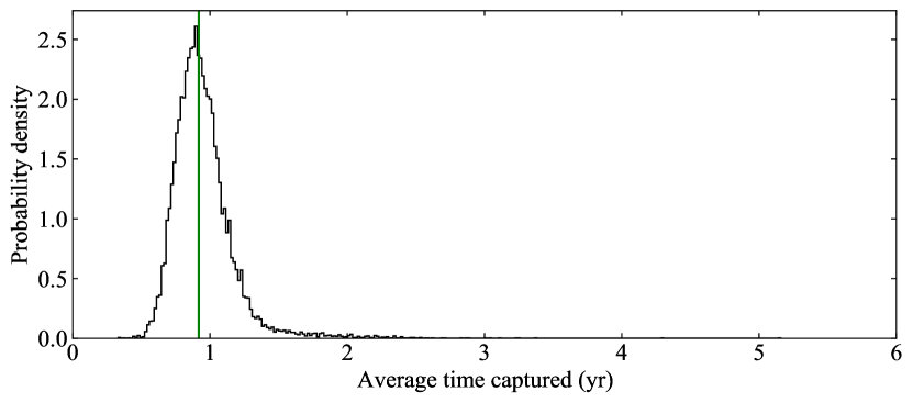
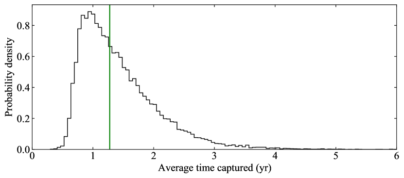
Figure 14: Distribution of average durations of temporary captures by Jupiter. Upper panel: For 2020 MK₄, 29P/Schwassmann-Wachmann 1 (second to upper panel), P/2008 CL94 (Lemmon) (second to bottom panel), and P/2010 TO20 (LINEAR-Grauer) (bottom panel). Median values are displayed as vertical green lines. The bins were computed using the Freedman and Diaconis rule implemented in NumPy (van der Walt et al. 2011; Harris et al. 2020). In the histogram, we use counts to form a probability density so the area under the histogram will sum to one.

In general, (temporary or long-term) capture (by Jupiter) is a very low probability event. On the other hand, the fact that close encounters between 2020 MK₄ and 29P may have taken place when one or both of these objects were temporary satellites of Jupiter opens the door to an alternative dynamical scenario for the origin of 2020 MK₄, that of a release by 29P with the gravitational assistance of Jupiter during a capture episode. Such a scenario has been observed in the past, for example the tidal disruption suffered by comet Shoemaker-Levy 9 in 1992 (see for example Nakano et al. 1993). Comet Shoemaker-Levy 9 was a Jovian satellite prior to impact (Benner 1994; Benner & McKinnon 1995). With the available data, an origin for 2020 MK₄ during a tidal (or binary) disruption event triggered by Jupiter on 29P cannot be excluded. Binary comets are rare, but they are known to exist (Agarwal et al. 2017, 2020); comet 288P/(300163) 2006 VW₁₃₉ could even be a triple (Kim et al. 2020).

In order to gain a better understanding of the role of Jupiter on the evolution of the objects shown in Table 1, we performed a similar study for the pairs P/2008 CL94 (Lemmon) and 2020 MK₄ as well as P/2010 TO20 (LINEAR-Grauer) and 2020 MK₄. The middle and bottom panels of Figure 13 summarize our results that use initial conditions from Tables 5 and 6. Close flybys when one or both members of the pair were temporary satellites of Jupiter are found in both cases with respective probabilities of 0.023 and 0.026. The distributions of the durations of the observed temporary capture events are displayed in Fig. 14. For comparison, the jovicentric orbital periods of known satellites of Jupiter range from slightly above 7 h (for Metis) to 2.17 yr (for S/2003 J 23).

The topic of temporary capture of cometary objects by Jupiter has already been studied in the past (see for example Carusi & Valsecchi 1981). Most known Jovian satellites have orbital periods close to 2 yr and move along very elongated and inclined paths (Sheppard & Jewitt 2003) so the objects discussed here may not complete one revolution around Jupiter before returning to interplanetary space. Following Fedorets et al. (2017), we may consider these episodes as linked to temporarily-captured flybys, not temporarily-captured orbiters. Although temporarily-captured orbiter episodes in which the object completes one orbit around the planet are also possible.

As for the possible past orbital evolution of 2020 MK₄ neglecting the possibility that it may have had an origin within the 29P–P/2008 CL94–P/2010 TO20 cometary complex, the results of longer integrations using MCCM to generate initial conditions indicate (see Fig. 12, left panel) that the probability of 2020 MK₄ having been captured from interstellar space during the past 0.5 Myr could be 0.49$\pm$0.04. This result together with the previous one for the probability of ejection indicate that the orbital evolution of 2020 MK₄ was as unstable in the past as it will be in the future.

5 Discussion

The origin of objects, such as 2020 MK₄, was thought to be in the trans-Neptunian or Edgeworth-Kuiper belt (see for example Fernandez 1980; Levison & Duncan 1997), but it is now generally accepted that this population may have its source in the scattered belt (see for example Di Sisto et al. 2009; Brasser & Wang 2015; Di Sisto & Rossignoli 2020; Roberts & Muñoz-Gutiérrez 2021); however, it is also important to consider the analysis in Grazier et al. (2018). Although cometary activity (either continuous or in the form of outbursts) has been detected at 30.7 AU for C/1995 O1 (Hale-Bopp) (Szabó et al. 2011), at 28.1 AU for 1P/Halley (Hainaut et al. 2004), and at 23.7 AU for C/2017 K2 (PANSTARRS) (Jewitt et al. 2017), so far no member of the trans-Neptunian belt (cold or scattered) has been recognized as active (see for example Cabral et al. 2019). In addition to comets, the only group of distant minor bodies that includes known active objects is that of the centaurs.

According to JPL’s SBDB search engine, as of March 5, 2021, there have been 547 known centaurs (objects with orbits between Jupiter and Neptune, 5.5 AU $<a<$ 30.1 AU). The list of known active centaurs maintained by Y. R. Fernández includes 34 objects, not counting (523676) 2013 UL₁₀ (Mazzotta Epifani et al. 2018) and the one discussed here, 2020 MK₄. Therefore, about 6.6% of the known centaurs have been observed at some point losing mass and displaying a cometary physical appearance. Not counting 29P/Schwassmann-Wachmann 1, the first active centaur to be identified as such was 95P/Chiron (Hartmann et al. 1990). Outbursts are sometimes associated with the ejection of sizable fragments, as in the case of 174P/Echeclus (see for example Rousselot 2008; Kareta et al. 2019).

Figure 11 shows that the objects in Table 1 had a very chaotic dynamical past and that their future orbital evolution will be equally chaotic, including very close encounters with Jupiter and perhaps also Saturn. In addition, Fig. 13 indicates that these objects may have experienced relatively close mutual flybys and in some cases such close encounters may have taken place when one or both of the objects involved were temporarily trapped by Jupiter’s gravitational pull, as shown in Fig. 14. Therefore, Jupiter plays a central role in the dynamics of this group of objects.

In general, our results indicate that the evolution of these minor bodies can only be reliably predicted a few thousand years into the past or the future, which is consistent with the conclusions in the extensive study of Roberts & Muñoz-Gutiérrez (2021). Although Roberts & Muñoz-Gutiérrez (2021) argue that mean-motion resonances with the giant planets may stabilize some of the orbits in this region and they provide some examples, for the set of objects studied here, resonant behavior fails to appear or at least its strength is not enough to mitigate their chaotic orbital evolution. The dynamical behavior observed is compatible with that of the centaurs experiencing generalized diffusion as discussed by Bailey & Malhotra (2009). In addition, relatively close and recurrent encounters between these objects are possible, and they are not impeded by resonances. Temporary captures by Jupiter of these objects are also recurrent (see Fig. 15).

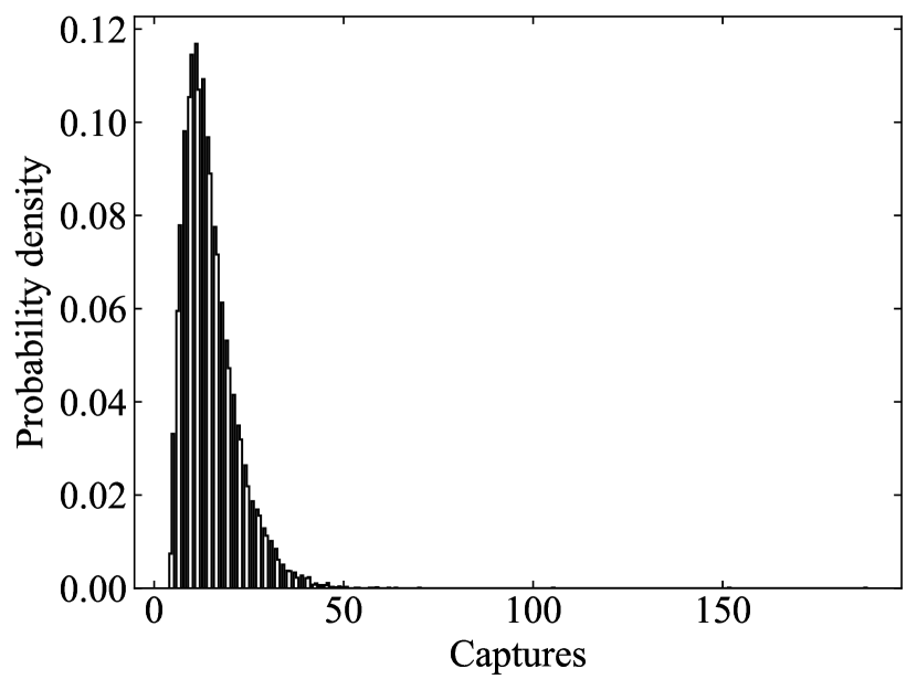
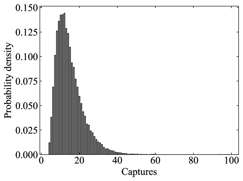
Figure 15: Distribution of the number of capture events by Jupiter per simulation. Upper panel: For 2020 MK₄ and for comet 29P/Schwassmann-Wachmann 1 (bottom panel). The bins were computed using the Freedman and Diaconis rule implemented in NumPy (van der Walt et al. 2011; Harris et al. 2020). In the histogram, we use counts to form a probability density so the area under the histogram will sum to one.

The orbital context analysis presented in Sect. 4.1 opens the possibility to close encounters between objects of this dynamical class as the mutual nodal distances are small. This theoretical possibility is confirmed by our $N$-body simulations, which indicate that close approaches at distances on the order of 10⁵ km (or 10^-3 AU) are indeed possible. However, this is the typical size of the coma of comet 29P when in outburst (see for example Trigo-Rodríguez et al. 2008) and this has the potential for a physical interaction between material in the comae of these objects during close encounters. This issue has never been considered before in the literature and it may accelerate the erosion rate of a cometary object as one active object may periodically penetrate the nebulous envelope of another and both experience mutual enhanced surface bombardment episodes.

Although our dynamical results cannot determine the origin of any of the objects studied in the scattered belt, they uncover an alternative or perhaps complementary scenario that may lead to increasing the population of objects following 29P-like orbits, that of the in situ production of these objects thanks to interactions with Jupiter of some precursor bodies. The existence of pairs of objects with small values of their mutual nodal distances and correlated orbits discussed in Sect. 4.1 provides additional support to this scenario when considering the very short dynamical lifetimes of these bodies.

As for the nature of the cometary-like activity of 2020 MK₄ presented in this paper, it seems to be irregular, not continuous. The data available from the Minor Planet Center (MPC, Rudenko 2016; Hernandez et al. 2019) indicate that its apparent magnitude went from $G=21.12$ mag on June 15, 2020, to $G=18.1$ mag on July 10, 2020, returning to $G=22.5$ mag by November 9, 2020. The data from the MPC suggest that the outburst may have stopped at some time between early September and November. Irregular activity is often found among centaurs (Jewitt 2009). Follow-up observations of this centaur are necessary to understand the nature of its activity.

6 Conclusions

In this paper, we have presented observations of 2020 MK₄ obtained with JKT and IAC80 which we have used to establish the active status of this centaur and to derive its colors. Its current orbital context has been outlined and its past, present, and future orbital evolution has been explored using direct $N$-body simulations. The object was originally selected to carry out this study because its orbit determination resembles that of comet 29P/Schwassmann-Wachmann 1 (see Table 1) and its first published observations hinted at an ongoing outburst event. Our conclusions can be summarized as follows.

1. We show that the PSF of 2020 MK₄ is nonstellar and this confirms the presence of cometary-like activity in the form of a conspicuous coma.

2. Centaur 2020 MK₄ is neutral-gray in color. The values of its color indexes, $(g^{\prime}-r^{\prime})=0.42\pm 0.04$ and $(r^{\prime}-i^{\prime})=0.17\pm 0.04$, are similar to the solar ones. These values are typical for active centaurs.

3. A lower limit for the absolute magnitude of the nucleus of 2020 MK₄ is $H_{g}=11.30\pm 0.03$ mag which, for an albedo in the range of 0.1–0.04, gives an upper limit for its size in the interval (23, 37) km.

4. The orbital evolution of 2020 MK₄ is very chaotic and it may eventually be ejected from the Solar System. It had a very chaotic dynamical past as well.

5. Both 2020 MK₄ and 29P may have been recurrent transient Jovian satellites. This also applies to P/2008 CL94 (Lemmon) and P/2010 TO20 (LINEAR-Grauer).

6. Although the past, present, and future dynamical evolution of 2020 MK₄ resembles that of 29P, a more robust orbit determination is needed to confirm or reject a possible relation between the two objects.

7. Our analyses suggest that active minor bodies may experience close encounters in which they traverse each other’s comae, experimenting mutual enhanced surface bombardment which may accelerate the erosion rate of these objects. Our analyses confirm that penetrating encounters in which 2020 MK₄ may travel across the coma of comet 29P are possible.

In summary, and based on the analysis of visible CCD images of 2020 MK₄, we confirm the presence of a coma of material around a central nucleus. Its surface colors place this centaur among the most extreme members of the gray group. Although the past, present, and future dynamical evolution of 2020 MK₄ resembles that of 29P, more data are required to confirm or reject a possible connection between the two objects and perhaps others.

Appendix A Mutual nodal distances and uncertainty estimates

The mutual nodal distance between two Keplerian trajectories with a common focus can be written as follows (see eqs. 16 and 17 in Saillenfest et al. 2017):

$${\Delta}_{\pm}=\frac{a_{2}\ (1-e_{2}^{2})}{1\pm e_{2}\ \cos{\varpi_{2}}}-\frac{a_{1}\ (1-e_{1}^{2})}{1\pm e_{1}\ \cos{\varpi_{1}}}\,,$$ (2)

where for prograde orbits the ”+” sign refers to the ascending node and the ”$-$” sign to the descending one, and

and

with $\Delta\Omega=\Omega_{2}-\Omega_{1}$, and $a_{j}$, $e_{j}$, $i_{j}$, $\Omega_{j}$, and $\omega_{j}$ ($j=1,2$) are the orbital elements of the orbits involved. In order to obtain the actual distributions of ${\Delta}_{\pm}$, we generated sets of orbital elements for the virtual objects using data from JPL’s SBDB. For example, the value of the semimajor axis of a virtual object was computed using the expression $a_{\rm v}=a+\sigma_{a}\,r_{\rm i}$, where $a$ is the semimajor axis, $\sigma_{a}$ is the standard deviation, and $r_{\rm i}$ is a (pseudo) random number with a normal distribution computed using NumPy (van der Walt et al. 2011; Harris et al. 2020). In order to calculate statistically relevant values of ${\Delta}_{\pm}$, we computed median and 16th and 84th percentiles from a set of 10⁴ pairs of virtual objects for each pair.

Appendix B Angular distances between pairs of orbital poles and perihelia

In order to understand the context of the orientations in space of the 29P-like orbits, we study the line of apsides of their paths and the projection of their orbital poles onto the plane of the sky. In heliocentric ecliptic coordinates, the longitude and latitude of an object at perihelion, $(l_{q},b_{q})$, are given by the following expressions: $\tan{(l_{q}-\Omega)}=\tan\omega\,\cos{i}$ and $\sin{b_{q}}=\sin\omega\,\sin{i}$ (see for example Murray & Dermott 1999). On the other hand, the ecliptic coordinates of the pole are $(l_{\rm p},b_{\rm p})=(\Omega-90\degr,90\degr-i)$. The angular distances between pairs of orbital poles and perihelia (see Fig. 6) are given by the angles $\alpha_{q}$ and $\alpha_{\rm p}$:

$$\cos{\alpha_{q}}=\cos{b_{q2}}\ \cos{b_{q1}}\ \cos{(l_{q2}-l_{q1})}+\sin{b_{q2}}\ \sin{b_{q1}}$$ (5)

and

$$\cos{\alpha_{\rm p}}=\cos{b_{\rm p2}}\ \cos{b_{\rm p1}}\ \cos{(l_{\rm p2}-l_{\rm p1})}+\sin{b_{\rm p2}}\ \sin{b_{\rm p1}}\,,$$ (6)

where the sets of orbital elements for the virtual objects were generated and the uncertainties were computed as described above.

Appendix C Input data

Here, we include the barycentric Cartesian state vectors of the four objects in Table 1. These vectors and their uncertainties were used to carry out the calculations discussed above and to generate the figures that display the time evolution of the various orbital parameters and the histograms of the close encounters of pairs of objects. For example, a new value for the $X$-component of the state vector was computed as $X_{\rm c}=X+\sigma_{X}\ r$, where $r$ is an univariate Gaussian random number, and $X$ and $\sigma_{X}$ are the mean value and its 1$\sigma$ uncertainty in the corresponding table.

Table 3: Barycentric Cartesian state vector of 2020 MK₄: Components and associated 1$\sigma$ uncertainties.

Component		value$\pm$1$\sigma$ uncertainty
$X$ (AU)	=	2.476823027013801$\times 10^{+0}$$\pm$2.63888043$\times 10^{-5}$
$Y$ (AU)	=	$-$5.649556533725540$\times 10^{+0}$$\pm$5.00052909$\times 10^{-5}$
$Z$ (AU)	=	$-$6.724625273177226$\times 10^{-1}$$\pm$6.68127413$\times 10^{-6}$
$V_{X}$ (AU/d)	=	6.344171798287663$\times 10^{-3}$$\pm$5.52645958$\times 10^{-7}$
$V_{Y}$ (AU/d)	=	2.598886274097145$\times 10^{-3}$$\pm$1.15080359$\times 10^{-6}$
$V_{Z}$ (AU/d)	=	2.738174058059657$\times 10^{-4}$$\pm$1.27180464$\times 10^{-7}$

Table 4: Barycentric Cartesian state vector of comet 29P/Schwassmann-Wachmann 1: Components and associated 1$\sigma$ uncertainties.

Component		value$\pm$1$\sigma$ uncertainty
$X$ (AU)	=	4.820127849857867$\times 10^{+0}$$\pm$2.26195239$\times 10^{-7}$
$Y$ (AU)	=	3.096547270522562$\times 10^{+0}$$\pm$2.26291332$\times 10^{-7}$
$Z$ (AU)	=	9.315292658149408$\times 10^{-1}$$\pm$1.80747737$\times 10^{-7}$
$V_{X}$ (AU/d)	=	$-$3.818139825384470$\times 10^{-3}$$\pm$2.98663624$\times 10^{-10}$
$V_{Y}$ (AU/d)	=	6.187940318090741$\times 10^{-3}$$\pm$1.63227588$\times 10^{-10}$
$V_{Z}$ (AU/d)	=	2.243304452195744$\times 10^{-4}$$\pm$2.29798018$\times 10^{-10}$

Table 5: Barycentric Cartesian state vector of comet P/2008 CL94 (Lemmon): Components and associated 1$\sigma$ uncertainties.

Component		value$\pm$1$\sigma$ uncertainty
$X$ (AU)	=	1.459836826464546$\times 10^{+0}$$\pm$2.48312839$\times 10^{-3}$
$Y$ (AU)	=	5.336008875429940$\times 10^{+0}$$\pm$8.60065292$\times 10^{-4}$
$Z$ (AU)	=	5.352334095577819$\times 10^{-1}$$\pm$3.08664106$\times 10^{-4}$
$V_{X}$ (AU/d)	=	$-$7.484540791199146$\times 10^{-3}$$\pm$4.84686920$\times 10^{-7}$
$V_{Y}$ (AU/d)	=	1.423074128372227$\times 10^{-3}$$\pm$3.12580298$\times 10^{-6}$
$V_{Z}$ (AU/d)	=	7.781756239073725$\times 10^{-4}$$\pm$3.54702110$\times 10^{-7}$

Table 6: Barycentric Cartesian state vector of comet P/2010 TO20 (LINEAR-Grauer): Components and associated 1$\sigma$ uncertainties.

Component		value$\pm$1$\sigma$ uncertainty
$X$ (AU)	=	$-$2.760378798588101$\times 10^{+0}$$\pm$1.87330516$\times 10^{-3}$
$Y$ (AU)	=	$-$4.981877686502737$\times 10^{+0}$$\pm$5.04623641$\times 10^{-4}$
$Z$ (AU)	=	$-$7.533566693101323$\times 10^{-2}$$\pm$7.13336260$\times 10^{-5}$
$V_{X}$ (AU/d)	=	6.530991396932470$\times 10^{-3}$$\pm$1.34995329$\times 10^{-6}$
$V_{Y}$ (AU/d)	=	$-$3.198756786861413$\times 10^{-3}$$\pm$1.72833828$\times 10^{-6}$
$V_{Z}$ (AU/d)	=	$-$2.946577560510802$\times 10^{-4}$$\pm$2.25495604$\times 10^{-8}$