Extremal Graphs for a Spectral Inequality on Edge-Disjoint Spanning Trees

Abstract.

Liu, Hong, Gu, and Lai proved if the second largest eigenvalue of the adjacency matrix of graph $G$ with minimum degree $\delta\geq 2m+2\geq 4$ satisfies $\lambda_{2}(G)<\delta-\frac{2m+1}{\delta+1}$, then $G$ contains at least $m+1$ edge-disjoint spanning trees, which verified a generalization of a conjecture by Cioabă and Wong. We show this bound is essentially the best possible by constructing $d$-regular graphs $\mathcal{G}_{m,d}$ for all $d\geq 2m+2\geq 4$ with at most $m$ edge-disjoint spanning trees and $\lambda_{2}(\mathcal{G}_{m,d})<d-\frac{2m+1}{d+3}$. As a corollary, we show that a spectral inequality on graph rigidity by Cioabă, Dewar, and Gu is essentially tight.

1. Introduction

Let $G=(V,E)$ be a finite, simple graph on $n$ vertices, and let $\lambda_{1}\geq\lambda_{2}\geq\cdots\geq\lambda_{n}$ and $\mu_{1}\leq\mu_{2}\leq\cdots\leq\mu_{n}$ be the eigenvalues of its adjacency and Laplacian matrices, respectively. Recall $\mu_{i}+\lambda_{i}=d$ for $d$-regular graphs [3, Ch. 1]. Additionally, let $\sigma(G)$ denote the maximum number of edge-disjoint spanning trees in $G$, sometimes referred to as the spanning tree packing number (see Palmer [20] for a survey of this parameter). Motivated by Kirchhoff’s celebrated matrix tree theorem on the number of spanning trees of a graph [14] and a question of Seymour [21], Cioabă and Wong [6] considered the relationship between the eigenvalues of a regular graph and $\sigma(G)$.

They obtained a result by combining two useful theorems. The Nash-Williams/Tutte theorem [19, 23] (described in Section 2.2) implies that if $G$ is a $(2m+2)$-edge-connected graph, then $\sigma(G)\geq m+1$. Additionally, Cioabă [4] showed if $G$ is a $d$-regular graph and $r$ is an integer with $2\leq r\leq d$ such that $\lambda_{2}(G)<d-2(r-1)/(d+1)$, then $G$ is $r$-edge-connected. These facts imply that if $G$ is a $d$-regular graph with $\lambda_{2}(G)<d-2(2m+1)/(d+1)$ for some integer $m$, with $2\leq m+1\leq\lfloor d/2\rfloor$, then $G$ contains $m+1$ edge-disjoint spanning trees. Cioabă and Wong conjectured the following factor of two improvement, which they verified for $m\in\{1,2\}$.

Conjecture 1 ([6]).

Let $m\geq 1$ be an integer and $G$ be a $d$-regular graph with $d\geq 2m+2$. If $\lambda_{2}(G)<d-\frac{2m+1}{d+1}$, then $\sigma(G)\geq m+1$.

This conjecture attracted much attention, leading to many partial results and generalizations [7, 8, 10, 11, 15, 17]. The question was ultimately resolved by Liu, Hong, Gu, and Lai.

Theorem 2 ([16]).

Let $m\geq 1$ be an integer and $G$ be a graph with minimum degree $\delta\geq 2m+2$. If $\lambda_{2}(G)<\delta-\frac{2m+1}{\delta+1}$, then $\sigma(G)\geq m+1$.

We show this bound is essentially the best possible.

Theorem 3.

For all $d\geq 2m+2\geq 4$, the $d$-regular graph $\mathcal{G}_{m,d}$ (defined in Section 2.1) has at most $m$ edge-disjoint spanning trees and satisfies

$$d-\dfrac{2m+1}{d+1}\leq\lambda_{2}(\mathcal{G}_{m,d})<d-\dfrac{2m+1}{d+3}.$$

Cioabă and Wong created special cases of this construction for the families $\mathcal{G}_{1,d}$ and (a slight variant of) $\mathcal{G}_{2,d}$ in [6] to show that Theorem 2 is essentially best possible for $m\in\{1,2\}$. In his PhD thesis [24], Wong also constructed the family $\mathcal{G}_{3,d}$ to show that Theorem 2 is essentially tight for $m=3$. Based on the family of graphs for the small cases of $m$ that appeared in [6], Gu [8] constructed a family of multigraphs by replacing every edge with multiple edges to show that the bounds in a multigraph analog of Theorem 2 are also the best possible. Additionally, Cioabă, Dewar, and Gu [5] used the variant of $\mathcal{G}_{2,d}$ from [6] to show that a sufficient spectral condition for graph rigidity is essentially the best possible. We generalize their result in Section 5.

In Section 2, we will construct the family of graphs $\mathcal{G}_{m,d}$ and prove the lower bound of Theorem 3. In Section 3, we will explicitly describe the characteristic polynomial of $\mathcal{G}_{m,d}$ (Theorem 11), and in Section 4, we will use the characteristic polynomial to prove the upper eigenvalue bound of Theorem 3. The proof of the second eigenvalue bound uses a classical number theoretic technique, Graeffe’s method (see Lemma 12), which to the best of our knowledge has not previously been used for second eigenvalue bounds. This approach should generalize to upper bounds on the roots of interesting combinatorial polynomials.

2. Graph Construction

2.1. Construction

We construct a family of graphs $\mathcal{G}_{m,d}$ such that $\lambda_{2}(\mathcal{G}_{m,d})<d-\frac{2m-1}{d+3}$, but $\sigma(\mathcal{G}_{m,d})\leq m$ for all $d\geq 2m+2\geq 4$. The graph $\mathcal{G}_{m,d}$ contains $2m+1$ copies of $K_{d+1}$, each with a deleted matching of size $m$. Then $m(2m+1)$ edges are added in a circulant manner to connect the vertices among the $2m+1$ cliques with the deleted matchings.

Let $d\geq 2m+2\geq 4$. The vertex set of $G=\mathcal{G}_{m,d}$ consists of all ordered pairs $(i,j)$ where $0\leq i\leq 2m$ and $0\leq j\leq d$. Let $H_{i}=\{(i,j)\mid 0\leq j\leq d\}$, and let the subgraph induced by $H_{i}$ be $G[H_{i}]=K_{d+1}\setminus E_{i}$, where

$$E_{i}=\{(i,2a-2)\sim(i,2a-1)\mid 1\leq a\leq m\}.$$

Now we connect edges among the $H_{i}$. Let

$$E^{\prime}=\{(i,2j+1)\sim(i+j+1,2j)\mid 0\leq i\leq 2m,\>0\leq j\leq m-1\},$$

where $i+j+1$ is taken modulo $2m+1$. Then

$$E(\mathcal{G}_{m,d})=\bigcup_{i=0}^{2m}E(G[H_{i}])\cup E^{\prime}.$$

This construction makes $\mathcal{G}_{m,d}$ a connected $d$-regular graph. See Figures 2.1 and 2.2.

2.2. Spanning Trees

Our result, like many prior results on edge-disjoint spanning trees, crucially relies on a theorem from Nash-Williams and Tutte, which converts a condition on $\sigma(G)$ to one on vertex partitions. If the vertex set $V(G)$ is partitioned into disjoint sets $V_{1},\ldots,V_{t}$, then let $e(V_{i},V_{j})$ be the number of edges with endpoints in both $V_{i}$ and $V_{j}$.

Theorem 4 (Nash-Williams/Tutte [19, 23]).

Let $G$ be a connected graph and $k>0$ be an integer. Then $\sigma(G)\geq k$ if and only if $\sum_{1\leq i<j\leq t}e(V_{i},V_{j})\geq k(t-1)$ for any partition $V(G)=V_{1}\cup\cdots\cup V_{t}$.

As in the previous subsection, let $H_{1},\ldots,H_{2m+1}$ be the modified cliques $K_{d+1}$ of $\mathcal{G}_{m,d}$. Since $e(H_{i},H_{j})=1$, we have

$$\sum_{0\leq i<j\leq 2m}e(H_{i},H_{j})=\dfrac{2m(2m+1)}{2}<(m+1)(2m).$$

By Theorem 4, $\mathcal{G}_{m,d}$ has at most $m$ edge-disjoint spanning trees. Then Theorem 2 implies $\lambda_{2}(\mathcal{G}_{m,d})\geq d-\frac{2m+1}{d+1}$, yielding the lower bound of Theorem 3. It remains to show $\lambda_{2}(\mathcal{G}_{m,d})<d-\frac{2m+1}{d+3}$.

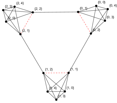
Figure 2.1. $\mathcal{G}_{1,4}$ with deleted dashed edges and labeled vertices.

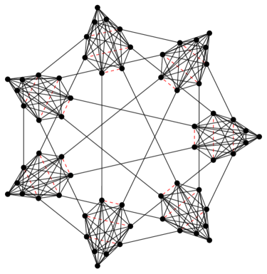
Figure 2.2. $\mathcal{G}_{3,8}$ with deleted dashed edges.

3. Characteristic Polynomial

The adjacency matrix of $\mathcal{G}_{m,d}$ is a block circulant matrix. Following [22], define $\operatorname{\mathcal{B}}(\mathbf{b}_{0},\mathbf{b}_{1},\ldots,\mathbf{b}_{n-1})$ to be the block circulant matrix

$$\begin{bmatrix}\mathbf{b}_{0}&\mathbf{b}_{1}&\mathbf{b}_{2}&\ddots&\mathbf{b}_{n-2}&\mathbf{b}_{n-1}\\ \mathbf{b}_{n-1}&\mathbf{b}_{0}&\mathbf{b}_{1}&\ddots&\mathbf{b}_{n-3}&\mathbf{b}_{n-2}\\ \mathbf{b}_{n-2}&\mathbf{b}_{n-1}&\mathbf{b}_{0}&\ddots&\mathbf{b}_{n-4}&\mathbf{b}_{n-3}\\ \ddots&\ddots&\ddots&\ddots&\ddots&\ddots\\ \mathbf{b}_{2}&\mathbf{b}_{3}&\mathbf{b}_{4}&\ddots&\mathbf{b}_{0}&\mathbf{b}_{1}\\ \mathbf{b}_{1}&\mathbf{b}_{2}&\mathbf{b}_{3}&\ddots&\mathbf{b}_{n-1}&\mathbf{b}_{0}\end{bmatrix},$$

where each $\mathbf{b}_{i}$ is a square matrix of equal dimension.

Lemma 5 ([22]).

The characteristic polynomial of a real, symmetric, block circulant matrix $\operatorname{\mathcal{B}}(\mathbf{b}_{0},\mathbf{b}_{1},\ldots,\mathbf{b}_{n-1})$ is given by

$$\det(xI-\operatorname{\mathcal{B}}(\mathbf{b}_{0},\mathbf{b}_{1},\ldots,\mathbf{b}_{n-1}))=\prod_{\zeta^{n}=1}\det(xI-\mathbf{H}_{\zeta}),$$

where

$$\mathbf{H}_{\zeta}=\mathbf{b}_{0}+\zeta\mathbf{b}_{1}+\cdots+\zeta^{n-1}\mathbf{b}_{n-1},$$

and $\zeta$ runs over the $n$th roots of unity (including $1$).

To determine the characteristic polynomial of $\mathcal{G}_{m,d}$, we will also need the following lemmas from linear algebra. Let $\mathbf{I}_{n}$ and $\mathbf{J}_{n}$ denote the identity matrix and all ones matrix of dimension $n$, respectively.

Lemma 6.

Let $\mathbf{A}$ be an invertible matrix and $\mathbf{u},\mathbf{v}$ be column vectors. Then,

$$\det(\mathbf{A}+\mathbf{uv}^{T})=(1+\mathbf{v}^{T}\mathbf{A}^{-1}\mathbf{u})\det(\mathbf{A}).$$

Lemma 7.

We have

$$\det(a\mathbf{I}_{n}+b\mathbf{J}_{n}) =a^{n}+na^{n-1}b,$$

$$(a\mathbf{I}_{n}+b\mathbf{J}_{n})^{-1} =\frac{1}{a}\mathbf{I}_{n}-\frac{b}{a(a+nb)}\mathbf{J}_{n}.$$

Finally, the characteristic polynomial of $\mathcal{G}_{m,d}$ will require defining the Chebyshev polynomials of the first kind $T_{n}(z)$ and Chebyshev polynomials of the second kind $U_{n}(z)$. We have [1, p. 775, Equations (22.3.6) and (22.3.7)]

(3.1) $$T_{n}(z) =\frac{n}{2}\sum_{k=0}^{\lfloor n/2\rfloor}\frac{(-1)^{k}}{n-k}\binom{n-k}{k}(2z)^{n-2k},$$

(3.2) $$U_{n}(z) =\sum_{k=0}^{\lfloor n/2\rfloor}{(-1)^{k}}\binom{n-k}{k}(2z)^{n-2k}.$$

They are also given by the implicit equations $T_{n}(\cos\theta)=\cos\left(n\theta\right)$ and $U_{n}(\cos\theta)\sin\theta=\sin((n+1)\theta)$. We prove a few lemmas on the Chebyshev polynomials and their connection to roots of unity.

Lemma 8.

For $m\geq 1$,

$$\frac{T_{2m+1}(z)}{z}=2^{2m}\prod_{j=1}^{m}\left(z^{2}-\sin^{2}\left(\dfrac{\pi j}{2m+1}\right)\right).$$

Proof.

Abramowitz and Stegun [1, Page 787, Equation 22.16.4] provide the zeroes of $T_{n}(z)$ as $\cos\left(\frac{2\ell-1}{2n}\pi\right),1\leq\ell\leq n$. The leading coefficient of $T_{2m+1}(z)$ is $2^{2m}$, as can be seen from equation (3.1), giving the product representation

$$T_{2m+1}(z) =2^{2m}\prod_{\ell=1}^{2m+1}\left(z-\cos\left(\frac{\ell-1/2}{2m+1}\pi\right)\right)$$

$$=2^{2m}z\prod_{\ell=1}^{m}\left(z-\cos\left(\frac{\ell-1/2}{2m+1}\pi\right)\right)\left(z+\cos\left(\frac{\ell-1/2}{2m+1}\pi\right)\right)$$

$$=2^{2m}z\prod_{\ell=1}^{m}\left(z^{2}-\sin^{2}\left(\frac{\ell-m-1}{2m+1}\pi\right)\right)$$

$$=2^{2m}z\prod_{\ell=1}^{m}\left(z^{2}-\sin^{2}\left(\frac{\ell}{2m+1}\pi\right)\right).$$

∎

Lemma 9.

For $m\geq 1$ and any $(2m+1)$-th primitive root of unity $\zeta$,

$$\prod_{j=1}^{m}(x^{2}+2x-1+\zeta^{j}+\overline{\zeta^{j}}) =\dfrac{T_{2m+1}(z)}{z},$$

$$\sum_{j=1}^{m}\dfrac{2x+\zeta^{j}+\overline{\zeta^{j}}}{x^{2}+2x-1+\zeta^{j}+\overline{\zeta^{j}}} =-\dfrac{1}{2z}+\dfrac{2m+1}{2T_{2m+1}(z)}(T_{2m+1}(z)-(z-1)U_{2m}(z)),$$

with the change of variables $z=\frac{x+1}{2}$.

Proof.

Applying Lemma 8,

$$\prod_{j=1}^{m}(x^{2}+2x-1+\zeta^{j}+\overline{\zeta^{j}}) =2^{2m}\prod_{j=1}^{m}\left(\left(\frac{x+1}{2}\right)^{2}-\left(\frac{\zeta^{j/2}-{\overline{\zeta^{j/2}}}}{2\imath}\right)^{2}\right)$$

$$=2^{2m}\prod_{j=1}^{m}\left(\left(\frac{x+1}{2}\right)^{2}-\sin^{2}\left(\frac{\pi j}{2m+1}\right)\right)$$

$$=\frac{T_{2m+1}\left(\frac{x+1}{2}\right)}{(x+1)/2}.$$

Also, we have

$$\sum_{j=1}^{m}\dfrac{2x+\zeta^{j}+\overline{\zeta^{j}}}{x^{2}+2x-1+\zeta^{j}+\overline{\zeta^{j}}} =\sum_{j=1}^{m}\frac{\frac{x+1}{2}-\left(\frac{\zeta^{j/2}-\overline{\zeta^{j/2}}}{2\imath}\right)^{2}}{\left(\frac{x+1}{2}\right)^{2}-\left(\frac{\zeta^{j/2}-\overline{\zeta^{j/2}}}{2\imath}\right)^{2}}$$

(3.3) $$=\sum_{j=1}^{m}\frac{\frac{x+1}{2}-\sin^{2}\left(\frac{\pi j}{2m+1}\right)}{\left(\frac{x+1}{2}\right)^{2}-\sin^{2}\left(\frac{\pi j}{2m+1}\right)}.$$

Taking a logarithm in Lemma 8 and then differentiating gives

$$\log T_{2m+1}(z)-\log z =\log 2^{2m}+\sum_{j=1}^{m}\log\left(z^{2}-\sin^{2}\left(\dfrac{\pi j}{2m+1}\right)\right),$$

(3.4) $$\dfrac{(2m+1)U_{2m}(z)}{T_{2m+1}(z)}-\frac{1}{z} =2z\sum_{j=1}^{m}\frac{1}{z^{2}-\sin^{2}\left(\frac{\pi j}{2m+1}\right)},$$

where we used $T^{\prime}_{n}(z)=nU_{n-1}(z)$ for $n\geq 1$. This can be verified from the series expansions of both. Substituting equation (3.4) into equation (3.3) with $z=(x+1)/2$ gives

$$\sum_{j=1}^{m}\frac{z-\sin^{2}\left(\frac{\pi j}{2m+1}\right)}{z^{2}-\sin^{2}\left(\frac{\pi j}{2m+1}\right)} =\sum_{j=1}^{m}\frac{z^{2}-\sin^{2}\left(\frac{\pi j}{2m+1}\right)}{z^{2}-\sin^{2}\left(\frac{\pi j}{2m+1}\right)}+\sum_{j=1}^{m}\frac{z-z^{2}}{z^{2}-\sin^{2}\left(\frac{\pi j}{2m+1}\right)}$$

$$=m+(z-z^{2})\sum_{j=1}^{m}\frac{1}{z^{2}-\sin^{2}\left(\frac{\pi j}{2m+1}\right)}$$

$$=m+\frac{(1-z)(2m+1)}{2}\frac{U_{2m(z)}}{T_{2m+1}(z)}-\frac{1-z}{2z}$$

$$=-\frac{1}{2z}+\frac{2m+1}{2T_{2m+1}(z)}\left(T_{2m+1}(z)-(z-1)U_{2m}(z)\right).$$

∎

We generalize Lemma 9 for all roots of unity $\zeta$.

Lemma 10.

For $m\geq 1$ and $2m+1\geq t\geq 1$, let $\zeta=e^{2\pi\imath t/(2m+1)}$ be a $(2m+1)$-th root of unity, where $\imath=\sqrt{-1}$. Define $g=\gcd(2m+1,t)$ and $n=\frac{2m+1}{g}$. Then

$$\prod_{j=1}^{m}(x^{2}+2x-1+\zeta^{j}+\overline{\zeta^{j}}) =\dfrac{(2T_{n}(z))^{g}}{2z},$$

$$\sum_{j=1}^{m}\dfrac{2x+\zeta^{j}+\overline{\zeta^{j}}}{x^{2}+2x-1+\zeta^{j}+\overline{\zeta^{j}}} =-\dfrac{1}{2z}+\dfrac{2m+1}{2T_{n}(z)}(T_{n}(z)-(z-1)U_{n-1}(z)),$$

with the change of variables $z=\frac{x+1}{2}$.

Proof.

Note that $\zeta$ is a primitive $n$th root of unity. By Lemma 9,

$$\prod_{j=1}^{\frac{n-1}{2}}(x^{2}+2x-1+\zeta^{j}+\overline{\zeta^{j}}) =\dfrac{T_{n}(z)}{z},$$

$$\sum_{j=1}^{\frac{n-1}{2}}\dfrac{2x+\zeta^{j}+\overline{\zeta^{j}}}{x^{2}+2x-1+\zeta^{j}+\overline{\zeta^{j}}} =-\dfrac{1}{2z}+\dfrac{2m+1}{2T_{n}(z)}(T_{n}(z)-(z-1)U_{n-1}(z)).$$

Notice $m=\frac{g-1}{2}n+\frac{n-1}{2}$. Using the periodicity of roots of unity several times,

$$\prod_{j=1}^{m}(x^{2}+2x-1+\zeta^{j}+\overline{\zeta^{j}}) =\left(\prod_{j=1}^{n}(x^{2}+2x-1+\zeta^{j}+\overline{\zeta^{j}})\right)^{\frac{g-1}{2}}\left(\prod_{j=1}^{\frac{n-1}{2}}(x^{2}+2x-1+\zeta^{j}+\overline{\zeta^{j}})\right)$$

$$=\left(\prod_{j=1}^{\frac{n-1}{2}}(x^{2}+2x-1+\zeta^{j}+\overline{\zeta^{j}})\right)^{g}(x^{2}+2x+1)^{\frac{g-1}{2}}$$

$$=\left(\dfrac{T_{n}(z)}{z}\right)^{g}(x+1)^{g-1}$$

$$=\dfrac{(2T_{n}(z))^{g}}{2z}.$$

Similarly,

$$\sum_{j=1}^{m}\dfrac{2x+\zeta^{j}+\overline{\zeta^{j}}}{x^{2}+2x-1+\zeta^{j}+\overline{\zeta^{j}}} =g\sum_{j=1}^{\frac{n-1}{2}}\dfrac{2x+\zeta^{j}+\overline{\zeta^{j}}}{x^{2}+2x-1+\zeta^{j}+\overline{\zeta^{j}}}+\dfrac{g-1}{2}\dfrac{2x+2}{x^{2}+2x+1}$$

$$=g\left(-\dfrac{1}{2z}+\dfrac{n}{2T_{n}(z)}(T_{n}(z)-(z-1)U_{n-1}(z))\right)+\dfrac{g-1}{x+1}$$

$$=-\dfrac{1}{2z}+\dfrac{2m+1}{2T_{n}(z)}(T_{n}(z)-(z-1)U_{n-1}(z)).$$

∎

Finally, we compute the characteristic polynomial of $\mathcal{G}_{m,d}$. Denote $\mathbf{J}_{a,b}$ to be the $a\times b$ all ones matrix.

Theorem 11.

For $d\geq 2m+2\geq 4$, the characteristic polynomial $p(x)$ of $\mathcal{G}_{m,d}$ is

$$(x+1)^{(d-2m)(2m+1)}\prod_{j=1}^{2m+1}(2T_{n}(z))^{g-1}\left[\left(-2m+1+\dfrac{2m-d}{z}\right)T_{n}(z)+(2m+1)(z-1)U_{n-1}(z)\right],$$

with the change of variables $g=\gcd(2m+1,j)$, $n=\frac{2m+1}{g}$, and $z=\frac{x+1}{2}$.

Proof.

By the symmetric construction of $\mathcal{G}_{m,d}$, its adjacency matrix is a block circulant matrix $\mathcal{B}(\mathbf{b}_{0},\ldots,\mathbf{b}_{2m})$. For any $i\neq j$, there is only one edge between $H_{i}$ and $H_{j}$. Then for $1\leq i\leq m$, $\mathbf{b}_{i}$ is a matrix with a single entry of $1$ in position $(2i,2i-1)$. Moreover, $\mathbf{b}_{i}=\mathbf{b}_{2m+1-i}^{T}$ for $m+1\leq i\leq 2m$. Finally, $\mathbf{b}_{0}$ is the adjacency matrix of any $H_{i}$. That is,

$$\mathbf{b}_{0}=\mathbf{J}_{d+1}-\mathbf{I}_{d+1}-\sum_{i=1}^{2m}\mathbf{b}_{i}.$$

By Lemma 5, the eigenvalues of the adjacency matrix are the union of the eigenvalues of each

$$\mathbf{H}_{\zeta} =\mathbf{b}_{0}+\zeta\mathbf{b}_{1}+\cdots+\zeta^{2m}\mathbf{b}_{2m}$$

$$=\begin{bmatrix}\mathbf{A}&\mathbf{J}_{2m,d-2m+1}\\ \mathbf{J}_{d-2m+1,2m}&\mathbf{J}_{d-2m+1}-\mathbf{I}_{d-2m+1}\end{bmatrix},$$

where $\zeta$ is a $(2m+1)$-th root of unity and

$$\mathbf{A}=\mathbf{J}_{2m}+\begin{bmatrix}-1&\overline{\zeta}-1\\ \zeta-1&-1\\ &&-1&\overline{\zeta^{2}}-1\\ &&\zeta^{2}-1&-1\\ &&&&\ddots\\ &&&&&-1&\overline{\zeta^{m}}-1\\ &&&&&\zeta^{m}-1&-1\end{bmatrix}.$$

The characteristic polynomial $p(x)$ is

$$p(x)=\prod_{\zeta^{2m+1}=1}\det(x\mathbf{I}-\mathbf{H}_{\zeta}).$$

We need the block determinant

$$\det(x\mathbf{I}-\mathbf{H}_{\zeta})=\begin{vmatrix}x\mathbf{I}_{2m}-\mathbf{A}&-\mathbf{J}_{2m,d-2m+1}\\ -\mathbf{J}_{d-2m+1,2m}&(x+1)\mathbf{I}_{d-2m+1}-\mathbf{J}_{d-2m+1}\end{vmatrix}.$$

Label the blocks $\mathbf{A}^{\prime},\mathbf{B},\mathbf{C},\mathbf{D}$. Passing to the Schur complement,

(3.5) $$\det(x\mathbf{I}-\mathbf{H}_{\zeta})=\det(\mathbf{D})\det(\mathbf{A}^{\prime}-\mathbf{BD}^{-1}\mathbf{C}).$$

By Lemma 7,

(3.6) $$\det\mathbf{D} =(x+1)^{d-2m}(x-d+2m),$$

$$\mathbf{D}^{-1} =\frac{1}{x+1}\mathbf{I}+\frac{1}{(x+1)(x-d+2m)}\mathbf{J}.$$

Note $\mathbf{J}_{n,m}\mathbf{J}_{m,l}=m\mathbf{J}_{n,l}$. Then,

$$\mathbf{BD}^{-1}\mathbf{C} =\frac{d-2m+1}{x+1}\mathbf{J}+\frac{(d-2m+1)^{2}}{(x+1)(x-d+2m)}\mathbf{J}=\frac{d-2m+1}{x-d+2m}\mathbf{J},$$

$$\mathbf{A}^{\prime}-\mathbf{BD}^{-1}\mathbf{C} =-\frac{x+1}{x-d+2m}\mathbf{J}+\begin{bmatrix}x+1&1-\overline{\zeta}\\ 1-\zeta&x+1\\ &&x+1&1-\overline{\zeta^{2}}\\ &&1-\zeta^{2}&x+1\\ &&&&\ddots\\ &&&&&x+1&1-\overline{\zeta^{m}}\\ &&&&&1-\zeta^{m}&x+1\\ \end{bmatrix}.$$

Let $\mathbf{M}_{\zeta}$ be the block matrix summand of $\mathbf{A}^{\prime}-\mathbf{BD}^{-1}\mathbf{C}$ and $\mathbf{u}$ be the all ones vector of dimension $2m$. Notice that $\mathbf{u}\mathbf{u}^{T}=\mathbf{J}_{2m}$, so that we can apply Lemma 6 to give

(3.7) $$\det(\mathbf{A}^{\prime}-\mathbf{BD}^{-1}\mathbf{C})=\left(1-\dfrac{x+1}{x-d+2m}\mathbf{u}^{T}\mathbf{M}_{\zeta}^{-1}\mathbf{u}\right)\det\mathbf{M}_{\zeta}.$$

Here, $\mathbf{u}^{T}\mathbf{M}_{\zeta}^{-1}\mathbf{u}$ gives the sum of the entries of $\mathbf{M}_{\zeta}^{-1}$. The inverse of a block diagonal matrix is the block diagonal matrix of the inverses of the blocks. Then the $j$th block of $\mathbf{M}_{\zeta}^{-1}$ is

$$\dfrac{1}{x^{2}+2x-1+\zeta^{j}+\overline{\zeta^{j}}}\begin{bmatrix}x+1&\overline{\zeta^{j}}-1\\ \zeta^{j}-1&x+1\end{bmatrix},$$

and

$$\mathbf{u}^{T}\mathbf{M}_{\zeta}^{-1}\mathbf{u}=\sum_{j=1}^{m}\dfrac{2x+\zeta^{j}+\overline{\zeta^{j}}}{x^{2}+2x-1+\zeta^{j}+\overline{\zeta^{j}}}.$$

The determinant of a block diagonal matrix is the product of the blocks’ determinants, so

$$\det\mathbf{M}_{\zeta}=\prod_{j=1}^{m}(x^{2}+2x-1+\zeta^{j}+\overline{\zeta^{j}}).$$

By Lemma 10,

$$\mathbf{u}^{T}\mathbf{M}_{\zeta}^{-1}\mathbf{u} =-\dfrac{1}{2z}+\dfrac{2m+1}{2T_{n}(z)}(T_{n}(z)-(z-1)U_{n-1}(z)),$$

$$\det\mathbf{M}_{\zeta} =\dfrac{(2T_{n}(z))^{g}}{2z}.$$

Substituting into (3.7), we obtain

$$\det(\mathbf{A^{\prime}}-\mathbf{BD}^{-1}\mathbf{C})=\dfrac{(2T_{n}(z))^{g-1}}{x-d+2m}\left[\left(-2m+1+\dfrac{2m-d}{z}\right)T_{n}(z)+(2m+1)(z-1)U_{n-1}(z)\right].$$

With (3.6), we simplify (3.5) to

$$\det(x\mathbf{I}-\mathbf{H}_{\zeta})=(x+1)^{d-2m}(2T_{n}(z))^{g-1}\left[\left(-2m+1+\dfrac{2m-d}{z}\right)T_{n}(z)+(2m+1)(z-1)U_{n-1}(z)\right].$$

Taking the product of $\det(x\mathbf{I}-\mathbf{H}_{\zeta})$ over all $2m+1$ roots of unity $\zeta$ yields the characteristic polynomial. ∎

4. Bounding the second eigenvalue

Let $[z^{n}]f(z)$ denote the coefficient of $z^{n}$ in $f(z)$, and let $z_{0}\geq z_{1}\geq\cdots\geq z_{n-1}$ be the roots of $f(z)$. Given any monic polynomial $f(z)$, we can rewrite $f(z)$ as

$$f(z)=\sum_{j=0}^{n}a_{j}z^{j}=\prod_{j=0}^{n-1}(z-z_{j})=z^{n}-z^{n-1}\sum_{j=0}^{n-1}z_{j}+O(z^{n-2}).$$

Lemma 12 (Graeffe’s Method [13]).

The largest root of a monic polynomial $f(z)=\sum_{j=0}^{n}a_{j}z^{j}$ can be bounded by

(4.1) $$z_{0}\leq\left(-4a_{n-4}+4a_{n-3}a_{n-1}+2a_{n-2}^{2}-4a_{n-2}a_{n-1}^{2}+a_{n-1}^{4}\right)^{1/4}.$$

Proof.

We compute

$$f(z)f(-z)=\prod_{j=0}^{n-1}(z-z_{j})(z+z_{j})=\prod_{j=0}^{n-1}(z^{2}-z_{j}^{2})=z^{2n}-z^{2n-2}\sum_{j=0}^{n-1}z_{j}^{2}+O(z^{2n-4}).$$

We know that this is an even function, so $a_{2n-1}=0$. Similarly, we can then compute

$$f(z)f(-z)f(\imath z)f(-\imath z) =\prod_{j=0}^{n-1}(z-z_{j})(z+z_{j})(z-\imath z_{j})(z+\imath z_{j})=\prod_{j=0}^{n-1}(z^{4}-z_{j}^{4})$$

$$=z^{4n}-z^{4n-4}\sum_{j=0}^{n-1}z_{j}^{4}+O(z^{4n-8}).$$

We conclude that

$$z_{0}\leq\left(\sum_{j=0}^{n-1}z_{j}^{4}\right)^{1/4}=\left(-[z^{4n-4}]f(z)f(-z)f(\imath z)f(-\imath z)\right)^{1/4}.$$

Moreover, only the powers of $z$ with degree at least $n-4$ multiply to produce a term of degree $4n-4$. By explicitly multiplying these polynomials out, we then have

$$f(z)f(-z) f(\imath z)f(-\imath z)$$

$$=\prod_{k=1}^{4}\left((\imath^{k}z)^{n}+a_{n-1}(\imath^{k}z)^{n-1}+a_{n-2}(\imath^{k}z)^{n-2}+a_{n-3}(\imath^{k}z)^{n-3}+a_{n-4}(\imath^{k}z)^{n-4}+O(z^{n-5})\right)$$

$$=z^{4n}-z^{4n-4}\left(-4a_{n-4}+4a_{n-3}a_{n-1}+2a_{n-2}^{2}-4a_{n-2}a_{n-1}^{2}+a_{n-1}^{4}\right)+O(z^{4n-8}).$$

∎

The intuition behind why Graeffe’s method suffices here is that if the polynomial’s roots are well separated, then Graeffe’s method provides extremely precise approximations. Here, numerically we observed $d-1\leq\lambda_{2}\leq d$ while the other roots were contained in $[-3,1]$. Then, passing to fourth powers using Graeffe’s method, the sum of fourth powers of all the roots is dominated by $\lambda_{2}^{4}$, so that taking a fourth root then provides a tight upper bound on the largest eigenvalue. We can use the same technique to derive a series of increasingly strong bounds on the largest root, as we incorporate more of the leading coefficients. For an introduction to the general method, see [13]. For historical discussion of the origin of the name and method, see [12].

We require the following technical inequality.

Lemma 13.

For $d\geq 2m+2\geq 6$, we have

$$\left(d^{4}+4d^{3}-(8m-2)d^{2}+4d+8m^{2}+4m+1\right)^{1/4}<d-\frac{2m+1}{d+3}+1.$$

Proof.

Let $n=2m+1$ and $\ell=d+1$, so this statement reduces to showing

$$\ell^{4}-4\ell^{2}n+2n^{2}-6n+8\ell n<\left(\ell-\frac{n}{\ell+2}\right)^{4}$$

for $\ell\geq n+2\geq 7$. By clearing denominators, expanding, and dividing through by $n$, this is equivalent to showing

$$2\ell^{4}(2n-5)+8\ell^{3}(n-6)-4\ell^{2}(n^{2}+6n+12)-8\ell(n^{2}+8n-8)+n^{3}-32n+96>0.$$

Note that $n^{3}-32n+96>0$ for $n\geq 5$, so we drop this term completely and divide by $2\ell$. It is left to show that

$$\ell^{3}(2n-5)+4\ell^{2}(n-6)+2\ell(-n^{2}-6n-12)+4(-n^{2}-8n+8)\geq 0.$$

Since we have $\ell-2\geq n\geq 5$, we can lower bound the left-hand side as

$$\geq\ell^{3}(10-5)+4\ell^{2}(5-6)+2\ell\left(-(\ell-2)^{2}-6(\ell-2)-12\right)+4\left(-(\ell-2)^{2}-8(\ell-2)+8\right)$$

$$=80-24\ell-12\ell^{2}+3\ell^{3}.$$

However, for $\ell\geq n+2\geq 7$, this polynomial is strictly positive. ∎

The main idea of our proof is to explicitly write down the first five coefficients of the characteristic polynomial, apply Graeffe’s method, and finally show that Graeffe’s method gives a slightly stronger bound than desired. We can now prove the following.

Theorem 14.

For $d\geq 2m+2\geq 4$,

$$d-\dfrac{2m+1}{d+1}\leq\lambda_{2}(\mathcal{G}_{m,d})<d-\dfrac{2m+1}{d+3}.$$

Proof.

See Section 2.1 for a discussion of the lower bound. Since $\mathcal{G}_{m,d}$ is a connected $d$-regular graph, it follows that $\lambda_{2}<\lambda_{1}=d$ [3, Ch. 1]. In the characteristic polynomial from Theorem 11, consider when $j=2m+1$ in the product. The expression in the product simplifies to

$$(x+1)^{2m}(x-d),$$

from which the eigenvalue of $d$ arises. Also observe that the factors $(x+1)^{(d-2m)(2m+1)}$ and $(2T_{n}(\frac{x+1}{2}))^{g-1}$ have roots in $[-3,1]$. It is enough to check that the factor

$$f_{n}(z)=\left(-2m+1+\dfrac{2m-d}{z}\right)T_{n}(z)+(2m+1)(z-1)U_{n-1}(z)$$

has roots less than $\frac{1}{2}({d-\frac{2m+1}{d+3}+1})$ for $1\leq j<2m+1$.

First, let us note some restrictions on the values of $n,m,d$ for which we need to prove this. The case $m=1$ was proven in [24]. Note that $n=(2m+1)/\gcd(2m+1,j)\neq 1$. As a divisor of $2m+1$, $n$ must then be odd, which eliminates $n=2$. We are left to check $2m+1\geq n\geq 3$ and $d\geq 2m+2$ for $m\geq 2$.

By (3.1) and (3.2), for $n\geq 4$

$$T_{n}(z) =2^{n-1}z^{n}-2^{n-3}nz^{n-2}+2^{n-6}n(n-3)z^{n-4}+O(z^{n-6}),$$

$$U_{n}(z) =2^{n}z^{n}-2^{n-2}(n-1)z^{n-2}+2^{n-5}(n-2)(n-3)z^{n-4}+O(z^{n-6}).$$

Then for $n\geq 4$,

$$f_{n}(z) =\left(-2m+1+\dfrac{2m-d}{z}\right)T_{n}(z)+(2m+1)(z-1)U_{n-1}(z)$$

$$=\left(-2m+1+\dfrac{2m-d}{z}\right)(2^{n-1}z^{n}-2^{n-3}nz^{n-2}+2^{n-6}n(n-3)z^{n-4}+O(z^{n-6}))$$

$$\quad+(2m+1)(z-1)(2^{n-1}z^{n-1}-2^{n-3}(n-2)z^{n-3}+2^{n-6}(n-3)(n-4)z^{n-5}+O(z^{n-6}))$$

so that the first five coefficients of the characteristic polynomial are explicitly

(4.2) $$\dfrac{f_{n}(z)}{2^{n}} =z^{n}-\dfrac{d+1}{2}z^{n-1}+\dfrac{2m+1-n}{4}z^{n-2}+\dfrac{dn+n-4m-2}{8}z^{n-3}$$

$$\quad+\dfrac{(n-4m-2)(n-3)}{32}z^{n-4}+O(z^{n-5}).$$

We examine the behavior at $n=3$, where (4.2) is technically undefined. Setting $n=3$ there, the $z^{n-4}$ factor vanishes due to the $(n-3)$ term, and we recover the correct polynomial. Therefore, we can extend the validity of this statement to $n\geq 3$.

By applying Graeffe’s method (Lemma 12) with

$$a_{n-1} =-\dfrac{d+1}{2},$$

$$a_{n-2} =\dfrac{2m+1-n}{4},$$

$$a_{n-3} =\dfrac{dn+n-4m-2}{8},$$

$$a_{n-4} =\dfrac{(n-4m-2)(n-3)}{32},$$

the largest root $z_{0}$ of $f_{n}(z)$ satisfies

(4.3) $$z_{0}\leq\dfrac{1}{2}\left(d^{4}+4d^{3}-(8m-2)d^{2}+4d+8m^{2}-8m+6n-5\right)^{1/4}.$$

Note that for fixed $m$ and $d$, this function is increasing in $n$ due to the $6n$ term, so it suffices to take $n=2m+1$ (the maximum possible value of $n$) in (4.3). Then (4.3) reduces to

(4.4) $$z_{0}\leq\dfrac{1}{2}\left(d^{4}+4d^{3}-(8m-2)d^{2}+4d+8m^{2}+4m+1\right)^{1/4}.$$

Lemma 13 shows that this is less than $\frac{1}{2}({d-\frac{2m+1}{d+3}+1})$ for $d\geq 2m+2\geq 6$. ∎

5. Application to Rigidity

One interesting application of this graph family pertains to graph rigidity. Rigidity is a well-studied notion of resistance to bending. A $k$-dimensional framework is a pair $(G,p)$, where $G$ is a graph and $p$ is a map from $V(G)$ to $\mathbb{R}^{k}$. Let $||\cdot||$ denote the Euclidean norm in $\mathbb{R}^{k}$. Two frameworks $(G,p)$ and $(G,q)$ are equivalent if $||p(u)-p(v)||=||q(u)-q(v)||$ for every edge $uv\in E(G)$, and congruent if $||p(u)-p(v)||=||q(u)-q(v)||$ for every $u,v\in V(G)$. Further, a framework $(G,p)$ is generic if the coordinates of its points are algebraically independent over the rationals. Finally, a framework $(G,p)$ is rigid if there exists an $\varepsilon>0$ such that if $(G,p)$ is equivalent to $(G,q)$ and $||p(u)-q(u)||<\varepsilon$ for every $u\in V(G)$, then $(G,p)$ is congruent to $(G,q)$. Note that we can consider rigidity as a property of the underlying graph, as a generic realization of $G$ is rigid in $\mathbb{R}^{k}$ if and only if every generic realization of $G$ is rigid in $\mathbb{R}^{k}$ [2]. Thus, we call a graph rigid in $\mathbb{R}^{k}$ if every generic realization of $G$ is rigid in $\mathbb{R}^{k}$. For the remainder of the section, we only consider rigid graphs in $\mathbb{R}^{2}.$

Cioabă, Dewar, and Gu investigated the connection between a graph’s Laplacian eigenvalues and rigidity, ultimately arriving at the following sufficient spectral condition.

Theorem 15 ([5]).

Let $G$ be a graph with minimum degree $\delta(G)\geq 6r$. If

1. $\mu_{2}(G)>\frac{6r-1}{\delta(G)+1}$,

2. $\mu_{2}(G-u)>\frac{4r-1}{\delta(G-u)+1}$ for every $u\in V(G)$, and

3. $\mu_{2}(G-v-w)>\frac{2r-1}{\delta(G-v-w)+1}$ for every $v,w\in V(G)$,

then $G$ contains at least $r$ edge-disjoint spanning rigid subgraphs.

Moreover, they used a variant of $\mathcal{G}_{2,d}$ and a result by Lovász and Yemini [18] to show that the first condition of the above theorem essentially cannot be improved for $r=1$. However, this categorization does not extend beyond $r=1$; we must turn to a more recent result by Gu [9] to verify tightness for larger values.

Suppose $\pi$ is a partition of $V(G)$. We call a part of $\pi$ trivial if it consists of a single vertex. Additionally, let $e_{G}(\pi)$ denote the number of edges of $G$ whose endpoints lie in two different parts of $\pi$.

Theorem 16 ([9]).

Let $r,\ell\geq 0$ be integers. If a graph $G$ contains $r$ spanning rigid subgraphs and $\ell$ spanning trees, all of which are mutually edge-disjoint, then for any partition $\pi$ of $V(G)$ with $t$ trivial parts,

$$e_{G}(\pi)\geq(3r+\ell)(|\pi|-1)-rt.$$

Using this result, we are able to prove the first condition of Theorem 15 is essentially tight for all $r\geq 1$.

Theorem 17.

Let $r>0$ be an integer. Then $\mathcal{G}_{3r-1,d}$ has fewer than $r$ edge-disjoint spanning rigid subgraphs and satisfies

$$\frac{6r-1}{d+3}<\mu_{2}(\mathcal{G}_{3r-1,d})\leq\frac{6r-1}{d+1}.$$

Proof.

Let $\pi$ be a partition of $V(\mathcal{G}_{3r-1,d})$, where the vertices of each modified $K_{d+1}$ form a part. Then $|\pi|=2(3r-1)+1=6r-1$ and $e_{\mathcal{G}_{3r-1,d}}(\pi)=(3r-1)(2(3r-1)+1)=(3r-1)(6r-1)$. Thus,

$$e_{\mathcal{G}_{3r-1,d}}(\pi)=(3r-1)(6r-1)<3r(6r-2)\leq(3r+\ell)((6r-1)-1)$$

for $\ell\geq 0$, so $\mathcal{G}_{3r-1,d}$ cannot contain $r$ edge-disjoint spanning rigid subgraphs by Theorem 16.

The spectral inequality is an immediate consequence of Theorem 3 by recognizing that $\mu_{2}=d-\lambda_{2}$, since the graph is $d$-regular. ∎

6. Open Problem

Numerically, $\lambda_{2}(\mathcal{G}_{m,d})$ converges to the upper bound $d-\frac{2m+1}{d+3}$ from Theorem 3. It is natural to ask the following: what is the optimal function $g(m,d)$ so that if a $d$-regular graph $\mathcal{G}$ has $\lambda_{2}(\mathcal{G})\leq g(m,d)$, then $G$ contains at least $m+1$ edge-disjoint spanning trees, and what are the extremal graphs?

7. Acknowledgements

The researach of Sebastian M. Cioabă was partially supported by NSF grants DMS-1600768 and CIF-1815922. Tanay Wakhare was supported by the MIT Television and Signal Processing Fellowship.

References

- [1] M. Abramowitz and I. A. Stegun. Handbook of mathematical functions with formulas, graphs, and mathematical tables, volume 55 of National Bureau of Standards Applied Mathematics Series. U.S. Government Printing Office, 1964.
- [2] L. Asimow and B. Roth. The rigidity of graphs. Transactions of the American Mathematical Society, 245:279–289, 1978.
- [3] A. E. Brouwer and W. H. Haemers. Spectra of graphs. Springer Science & Business Media, 2011.
- [4] S. M. Cioabă. Eigenvalues and edge-connectivity of regular graphs. Linear Algebra and its Applications, 432(1):458–470, 2010.
- [5] S. M. Cioabă, S. Dewar, and X. Gu. Spectral conditions for graph rigidity in the Euclidean plane. 2021. arXiv preprint arXiv:2001.06934.
- [6] S. M. Cioabă and W. Wong. Edge-disjoint spanning trees and eigenvalues of regular graphs. Linear Algebra and its Applications, 437(2):630–647, 2012.
- [7] X. Gu. Connectivity and spanning trees of graphs. PhD thesis, West Virginia University, 2013, available online at https://researchrepository.wvu.edu/cgi/viewcontent.cgi?article=6007&context=etd.
- [8] X. Gu. Spectral conditions for edge connectivity and packing spanning trees in multigraphs. Linear Algebra and its Applications, 493:82–90, 2016.
- [9] X. Gu. Spanning rigid subgraph packing and sparse subgraph covering. SIAM Journal on Discrete Mathematics, 32(2):1305–1313, 2018.
- [10] X. Gu, H. Lai, P. Li, and S. Yao. Edge-disjoint spanning trees, edge connectivity, and eigenvalues in graphs. Journal of Graph Theory, 81(1):16–29, 2016.
- [11] Y. Hong, X. Gu, H. Lai, and Q. Liu. Fractional spanning tree packing, forest covering and eigenvalues. Discrete Applied Mathematics, 213:219–223, 2016.
- [12] Alston S. Householder. Dandelin, Lobačevskiĭ, or Graeffe? Amer. Math. Monthly, 66:464–466, 1959.
- [13] C. A. Hutchinson. On Graeffe’s Method for the Numerical Solution of Algebraic Equations. Amer. Math. Monthly, 42(3):149–161, 1935.
- [14] G. Kirchhoff. Ueber die auflösung der gleichungen, auf welche man bei der untersuchung der linearen vertheilung galvanischer ströme geführt wird. Annalen der Physik, 148(12):497–508, 1847.
- [15] G. Li and L. Shi. Edge-disjoint spanning trees and eigenvalues of graphs. Linear Algebra and its Applications, 439(10):2784–2789, 2013.
- [16] Q. Liu, Y. Hong, X. Gu, and H. Lai. Note on edge-disjoint spanning trees and eigenvalues. Linear Algebra and its Applications, 458:128–133, 2014.
- [17] Q. Liu, Y. Hong, and H. Lai. Edge-disjoint spanning trees and eigenvalues. Linear Algebra and its Applications, 444:146–151, 2014.
- [18] L. Lovász and Y. Yemini. On generic rigidity in the plane. SIAM J. Algebraic Discrete Methods, 3(1):91–98, 1982.
- [19] C. St. J. A. Nash-Williams. Edge-disjoint spanning trees of finite graphs. Journal of the London Mathematical Society, 1(1):445–450, 1961.
- [20] E. M. Palmer. On the spanning tree packing number of a graph: a survey. Discrete Math., 230(1-3):13–21, 2001. Paul Catlin memorial collection (Kalamazoo, MI, 1996).
- [21] P. Seymour. Private communication to Sebastian Cioabă, April 2010.
- [22] G. J. Tee. Eigenvectors of block circulant and alternating circulant matrices. New Zealand J. Math., 36:195–211, 2007.
- [23] W. T. Tutte. On the problem of decomposing a graph into n connected factors. Journal of the London Mathematical Society, 1(1):221–230, 1961.
- [24] W. Wong. Spanning trees, toughness, and eigenvalues of regular graphs. PhD thesis, University of Delaware, 2013, available online at https://pqdtopen.proquest.com/doc/1443835286.html?FMT=ABS.