Isconna: Streaming Anomaly Detection with Frequency and Patterns

Abstract

An edge stream is a common form of presentation of dynamic networks. It can evolve with time, with new types of nodes or edges being continually added. Existing methods for anomaly detection rely on edge occurrence counts or compare pattern snippets found in historical records. In this work, we propose Isconna, which focuses on both the frequency and the pattern of edge records. The burst detection component targets anomalies between individual timestamps, while the pattern detection component highlights anomalies across segments of timestamps. These two components together produce three intermediate scores, which are aggregated into the final anomaly score. Isconna does not actively explore or maintain pattern snippets; it instead measures the consecutive presence and absence of edge records. Isconna is an online algorithm, it does not keep the original information of edge records; only statistical values are maintained in a few count-min sketches (CMS). Isconna’s space complexity $O(rc)$ is determined by two user-specific parameters, the size of CMSs. In worst case, Isconna’s time complexity can be up to $O(rc)$, but it can be amortized in practice. Experiments show that Isconna outperforms five state-of-the-art frequency- and/or pattern-based baselines on six real-world datasets with up to 20 million edge records.

Introduction

An edge stream, or a stream of edge records, represents a set of connections on a time-evolving graph. Unlike its static counterpart, in a stream, edge records reach the detection system one after another. Therefore, some statistical values for the whole dataset are not available as a priori; this causes problems in data preprocessing and other aspects.

In the real world, an edge stream can be used as the abstraction of various applications, such as network connections, social network posts. Within these streams, anomalies may occasionally appear, like distributed denial of service (DDoS) attacks in a network graph, breaking events in a social network graph, or money laundering in a transaction network. As an informal definition, anomalies in an edge stream are behaviors, represented as edges, that deviates from the usual pattern or are known to be harmful to the system’s regular operation. The goal of anomaly detection algorithms is to mark those anomalous behaviors, where a typical method is to assign a score to each edge record indicating the degree of anomalousness.

Existing methods, like SedanSpot, process each edge record individually without considering the contextual information. If edge records are extracted outside of the original context, the algorithm tends to produce the same result. However, in different environments, what should be regarded as anomalous are significantly different. The normal level of an industry network is unlikely to be the same as a home network. While recent methods take into account contextual information, they only focus on a specific attribute; for example, MIDAS uses the occurrence count for burst detection. In this work, as a preliminary attempt, we combine the characteristics of multiple contextual attributes, proposing the Isconna, a streaming anomaly detection algorithm focusing on both robustness and efficacy.

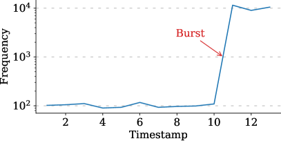
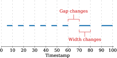
Figure 1: Example of bursts (left) and pattern changes (right)

Informally, a burst is a sudden change in the number of occurrences (frequency).

As an example, Fig. 1 (left) shows the number of outbound connections from a workstation within consecutive timestamps. Before timestamp 11, there are around 100 connections in each timestamp. From timestamp 11, it surges to about 10,000 and maintains in the following timestamps. Intuitively, we can believe something happens to the machine, e.g., the user account is compromised, or the network adapter is malfunctioning.

Likewise, the change of pattern may also indicate irregular events. Fig. 1 (right) gives an example. It represents whether a user visits a news website, and each timestamp is one day. Before day 60, the user visits the website for five consecutive days, then does not visit it for another five days, and loop. After day 60, the length of the consecutive visiting and non-visiting are both doubled. This potentially indicates some event occurs and changes the user’s reading habit.

Our algorithm is motivated by the burst and the pattern change. It learns the frequency, the consecutive occurrence and absence from the history data, then uses them to predict the anomalous degree of future data.

Existing methods in the streaming anomaly detection are briefly introduced in the next section. The details of the Isconna is given in the Proposed Algorithm section. The Experiments section demonstrates the performance of Isconna using various experiments with different conditions and configurations.

Related Works

Anomaly Detection is a vast topic by itself and cannot be fully covered in this manuscript. See (Chandola, Banerjee, and Kumar 2009) for an extensive survey on anomaly detection, and (Akoglu, Tong, and Koutra 2015) for a survey on graph-based anomaly detection.

OddBall (Akoglu, McGlohon, and Faloutsos 2010), CatchSync (Jiang et al. 2016) and (Kleinberg 1999) detect anomalous nodes. AutoPart (Chakrabarti 2004) spots anomalies by finding edge removals that significantly reduce the compression cost. NrMF (Tong and Lin 2011) detect anomalous edges by factoring the adjacency matrix and flagging edges with high reconstruction errors. FRAUDAR (Hooi et al. 2017) and k-cores (Shin, Eliassi-Rad, and Faloutsos 2018) target anomalous subgraphs detection, However, these approaches work on static graphs only.

Among methods that focus on dynamic graphs, DTA/STA (Sun, Tao, and Faloutsos 2006) approximate the adjacency matrix of the current snapshot using the matrix factorization. AnomRank (Yoon et al. 2019), which is inspired by PageRank (Page et al. 1999), iteratively updates two score vectors and compute anomaly scores. Copycatch (Beutel et al. 2013) and SpotLight (Eswaran et al. 2018) detect anomalous subgraphs. HotSpot (Yu et al. 2013), IncGM+ (Abdelhamid et al. 2017) and DenseAlert (Shin et al. 2017) utilize incremental method to process graph updates or subgraphs more efficiently. SPOT/DSPOT (Siffer et al. 2017) use the extreme value theory to automatically set thresholds for anomalies. However, these approaches work on graph snapshots only and are unable to handle the finer granularity of edge streams.

As for methods focusing on edge streams, RHSS (Ranshous et al. 2016) focuses on sparsely-connected parts of a graph. SedanSpot (Eswaran and Faloutsos 2018) identifies edge anomalies based on edge occurrence, preferential attachment, and mutual neighbors. MIDAS (Bhatia et al. 2020) identifies microcluster-based anomalies, or suddenly arriving groups of suspiciously similar edges. CAD (Sricharan and Das 2014) localizes anomalous changes in the graph structure using the commute time distance measurement. However, these methods are unable to detect any seasonality or periodic patterns in the data.

PENminer (Belth, Zheng, and Koutra 2020) explores the persistence of activity snippets, i.e., the length and regularity of edge-update sequences’ reoccurrences. F-FADE (Chang et al. 2021) aims to detect anomalous interaction patterns by factorizing the frequency of those patterns. These methods can effectively detect periodic patterns, but they require a considerable amount of time to explore and maintain possible patterns in the network.

Recently, several deep learning based methods have also been proposed for anomaly detection; see (Chalapathy and Chawla 2019) for an extensive survey. However, such approaches are unable to detect in a streaming manner.

Theory

Table of Notations

Due to the page limit, the table of notations is given in the supplementary.

Definitions

Edge Record

An edge record $e$ is an individual entry in the dataset. It is defined as an ordered tuple $(s,d,t)$. The array of all edge records sorted in non-descending order of timestamp is called an edge stream $\mathscr{S}$.

Edge Type

An edge type $e$ is an abstract edge without the timestamp $t$. It is defined as an ordered tuple $(s,d)$. The set of all edge types is the edge set $\mathscr{E}$.

Segment

A segment $g$, or $[t_{i},t_{j}]$ is an set of consecutive timestamps, defined as $\{t_{k}|t_{i}\leq t_{k}\leq t_{j}\}$. For a segment $[t_{i},t_{j}]$, if there is an edge type $e\coloneqq(s,d)$ additionally satisfies $\forall t\in[t_{i},t_{j}],\exists e\in\mathscr{S},s=s_{e}\land d=d_{e}\land t=t_{e}$, then the segment is called an occurrence segment of edge type $e$ on the interval $t_{i}$ to $t_{j}$, or an occurrence segment. Similarly, a segment is called an absence segment iff $\forall t\in[t_{i},t_{j}],\nexists e\in\mathscr{S},s=s_{e}\land d=d_{e}\land t=t_{e}$. In this work, we only consider non-expandable segments, that is, $[t_{i},t_{j}]$ is an occurrence segment or an absence segment, but neither $[t_{i}-1,t_{j}]$ nor $[t_{i},t_{j}+1]$ is. We additionally define $g(e)$ as the occurrence segment that contains edge record $e$ and $g(e,t)$ as the absence segment of edge type $e$ with timestamp $t$ included.

Problem 1 (Anomaly Detection)

Given an edge stream $\mathscr{S}$ on a time-evolving graph $G$, assign a score to each edge record $e$ according to the contextual information, where a higher score indicates a higher degree of anomalousness.

Proposed Anomalousness Measure

An anomalousness measure is a function that evaluates the anomalousness of a given edge record according to its internal states. Formally, $A(e;\theta)\coloneqq\mathscr{S}\times\Theta\to\mathbb{R}^{+}$, where $\theta\in\Theta$ is the contextual information maintained as the internal state of the detector, $\Theta$ is the set of all possible internal states, $A(\cdot)$ is the anomalousness measure. We first propose the combined form of the anomalousness measure

$$A(e;\theta)\coloneqq f(B(e;\theta),P(e;\theta))$$ (1)

where $B(\cdot)$ is a function that evaluates the burst anomalousness, $P(\cdot)$ is a function that evaluates pattern change anomalousness, and $f(\cdot)$ is a function that combines these components.

Burst Anomalousness Measure

For burst detection, we adopt the idea of the MIDAS algorithm, using a statistical hypothesis test to evaluate the degree of deviation from the learned mode. For simplicity, we derive the formula of anomalousness from the G-test. The comparison between the chi-squared test and the G-test is out of the scope of this work, a detailed discussion can be found at (Cressie and Read 1984).

$$G \coloneqq 2\sum_{i}O_{i}\cdot\log\dfrac{O_{i}}{E_{i}}$$

$$=2\left(O_{\text{current}}\cdot\log\dfrac{O_{\text{current}}}{E_{\text{current}}}+O_{\text{past}}\cdot\log\dfrac{O_{\text{past}}}{E_{\text{past}}}\right)$$

$$=2\left[c\cdot\log\dfrac{c}{\dfrac{a}{t-1}}+a\cdot\log\dfrac{a}{\dfrac{a}{t-1}\cdot(t-1)}\right]$$

$$=2c\cdot\log\left[\dfrac{c\cdot(t-1)}{a}\right]$$

where $G$ is the G-test statistic, $O_{i}$ is the observed count of class $i$, $E_{i}$ is the expected count of class $i$, $t$ is the timestamp of edge record $e$, $c$ is the current occurrence count of $e$ in timestamp $t$, $a$ is the accumulated occurrence count of $e$ up to timestamp $t-1$.

The derived statistic ranges from negative infinity to positive infinity. However, as an anomalousness measure, we only concern the extent of deviations. Hence, we take its absolute value. The formal definition of the burst anomalousness measure is given in Definition 1.

Definition 1 (Burst Anomalousness Measure)

Given an edge record $e\in\mathscr{S}$ and the detector’s internal state $\theta$, the burst anomalousness measure is defined as

$$B(e;\theta)\coloneqq \left|2c(e;\theta)\cdot\log\left[\dfrac{c(e;\theta)(t_{e}-1)}{a(e;\theta)}\right]\right|$$ (2)

$$c(e;\theta)\coloneqq \|\{e_{i}|e=e_{i},e_{i}\in\mathscr{S},t_{e_{i}}=t_{\theta}\}\|$$ (3)

$$a(e;\theta)\coloneqq \|\{e_{i}|e=e_{i},e_{i}\in\mathscr{S},t_{e_{i}}<t_{\theta}\}\|$$ (4)

where $B(e;\theta)$ is the burst anomalousness measure, $t_{e}$ is the timestamp of edge record $e$, $t_{\theta}$ is detector’s internal timestamp.

Pattern Change Anomalousness Measure

For pattern change detection, an intuitive idea is to maintain a portion of the history, then detect the repeated pattern. If we regard each edge record as a character and the maintained history as a string, this becomes the repeated substring pattern problem. For example, string “abcabcabcabc” is four repeats of substring “abc”. There are many different algorithms to solve this problem efficiently. However, as string comparison is unavoidable, it would be difficult, if not impossible, to decrease the time complexity below linear. Additionally, with the edge stream keeps evolving, the maintained records are also constantly updated. In the worst case, the above algorithm for detecting repeated patterns is executed whenever a new edge record reaches the system. On the other hand, the maintained stream history may be a combination of multiple patterns with different periods. As a result, such an exact pattern tracking solution may not be practical.

We try to use various methods to solve or bypass those problems. The first method is to track individual edge types rather than exact patterns. In theory, if there are $n$ edge types and the maximum pattern length is $m$, then the number of unique patterns would be $O(n^{m})$. Therefore, targeting edge types can significantly reduce the space complexity, and thus the time complexity.

The second method is to abstract patterns into several statistical values. We choose the length of patterns and the interval between pattern occurrences because they are easier to maintain. For simplicity, we call them width and gap, respectively. Note that we do not use the term “period”, because in the real world, patterns do not always have a strict period, but may have a rough range of intervals between occurrences. This method alone does not help solve the aforementioned problems. However, with different edge types being tracked separately, updating the maintained history is equivalent to modifying the recorded width and gap values of affected edge types.

As a quick summary, two statistical values, the length of consecutive edge type occurrences (width) and the interval between occurrences (gap), are used to compute the pattern change anomalousness, whose formula is not discussed yet.

For the formula of pattern change anomalousness measure, we still prefer the statistical hypothesis tests due to their high interpretability. To achieve this, we split the tracking of width and gap into the current and the historical values, and use the concept of segments to differentiate them. Table 1 shows those combinations and corresponding notations that will be used in the definition. The formal definition of the pattern change anomalousness measure is given in Definition 2.

Table 1: Notations of concept combinations

	Current	Accumulated
Occurrence	$c(g(e);\theta)$	$a(g(e);\theta)$
Absence	$c(g(e,t);\theta)$	$a(g(e,t);\theta)$

Definition 2 (Pattern Change Anomalousness Measure)

Given an edge record $e\in\mathscr{S}$ and the detector’s internal state $\theta$, the pattern change anomalousness measure is defined as

$$P(e;\theta)\coloneqq f(P(g(e);\theta),P(g(e,t^{\prime});\theta))$$ (5)

$$P(g;\theta)\coloneqq \left|2c(g;\theta)\cdot\log\left[\dfrac{c(g;\theta)(\bar{t}(g)-1)}{a(g;\theta)}\right]\right|$$ (6)

$$c(g;\theta)\coloneqq \|\{t|t\in g\}\|$$ (7)

$$a(g(e);\theta)\coloneqq \sum_{[t_{i},t_{j}]\in\mathscr{G}_{o}\backslash g(e),t_{j}<t_{e}}\|\{t|t\in[t_{i},t_{j}]\}\|$$ (8)

$$a(g(e,t);\theta)\coloneqq \sum_{[t_{i},t_{j}]\in\mathscr{G}_{a}\backslash g(e,t),t_{j}<t}\|\{t|t\in[t_{i},t_{j}]\}\|$$ (9)

where $P(e;\theta)$ is the pattern change anomalousness measure, $t^{\prime}$ is the largest timestamp that is smaller than the initial timestamp of $g(e)$, $\bar{t}(g)$ is the index number of $g$ , $\mathscr{G}_{o}$ is the set of occurrence segments, $\mathscr{G}_{a}$ is the set of absence segments.

Component Combinator

In Equation 1 and Equation 5, we use a combinator $f(\cdot)$ without giving its definition. Since the components defined above represent different aspects of the stream, they may not have the same scale. Thus we define $f(\cdot)$ as the product of components with exponential weights. The anomalousness measure can be therefore converted into the following formula.

$$A(e;\theta)\coloneqq B(e;\theta)^{\alpha}\cdot P(g(e);\theta)^{\beta}\cdot P(g(e,t^{\prime});\theta)^{\gamma}$$ (10)

where the exponents $\alpha,\beta,\gamma\in[0,+\infty)$ are the weight of components, depending on the goals of the actual scenario.

As a general guide, $\beta$ is usually greater than $\gamma$, because an occurrence segment includes the information about this edge type, while an absence segment is about other edge types and is already covered by their corresponding occurrence segments. For $\alpha$ vs. $\beta$, it depends on the characteristics of the edge stream. For example, in a stable scenario where fluctuations are relatively small, a higher $\alpha$ helps spot bursts that are difficult to notice. While in the scenario where edges follow strong patterns, users may prefer a high $\beta$ and $\gamma$ value to capture any abnormal changes.

Proposed Method: Isconna

In this section, we will describe the algorithm procedure and implementation details. Fig. 2 gives an overview of our proposed Isconna algorithm.

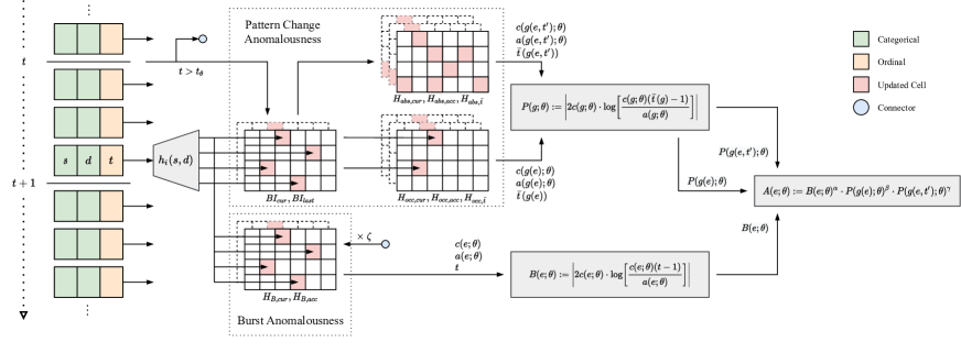
Figure 2: Overview of the Isconna algorithm

Count-Min Sketches

From Equation 10, we learn that for each edge record, the detector needs to compute the anomalousness measure for the three different components. As edges are tracked by edge types, ideally, the detector should maintain the information of each edge type independently. However, this is impractical due to the memory limit and the streaming nature.

To resolve this problem, we use Count-Min Sketches (CMS) (Cormode and Muthukrishnan 2004) to store the intermediate information. A CMS consists of a few hash tables with different hash functions but the same number of cells. In addition to the Hash, Add and Query operations provided by the original CMS, we also define the ArgQuery operation. A brief introduction to CMS is given in the supplementary.

For simplicity, we apply the Same-Layout Assumption to CMSs in the detector, that is, all CMSs share the same shape and the same group of hash functions, thus an item can be hashed into the same group of cells for all CMSs. In practice, this assumption reduces the number of required hashing operations and helps decrease the running time.

Busy Indicators

The tracking for the burst anomalousness measure is straightforward. As it only counts the number of occurrences, when an edge reaches the detector, it is hashed and the corresponding cells in CMSs increment by 1. However, for the pattern change anomalousness measure, it tracks the length of occurrence/absence segments, which requires special data structures to track the beginning and the ending of segments. Therefore, we propose a special type of CMS, Busy Indicators (BI).

A group of BIs consists of two CMSs with Boolean elements, one tracks the edge occurrence of the current timestamp, another for the last timestamp. All possible element combinations are listed in Table 2. Note that the beginning of an occurrence segment is at the same time the ending of the adjacent absence segment, and vice versa.

Table 2: Combination of BI element values

	$\top(>0)$	$\bot(=0)$
$\top(>0)$	Occ. cont.	Occ. init.
$\bot(=0)$	Abs. init.	Abs. cont.

Procedure

Algorithm 1 Isconna-EO ($\mathscr{S}$, $\zeta$, $\alpha$, $\beta$, $\gamma$)

1:Stream $\mathscr{S}$, scale factor $\zeta$, weight $\alpha$, $\beta$, $\gamma$

2:Anomalousness measure $A$

3:Initialize CMS $H_{B,cur}$, $H_{B,acc}$, $H_{occ,cur}$, $H_{occ,acc}$, $H_{occ,\bar{t}}$, $H_{abs,cur}$, $H_{abs,acc}$, $H_{abs,\bar{t}}$, $BI_{cur}$ and $BI_{last}$

4:Initialize internal state $\theta$ $\triangleright$ Including CMSs

5:for new edge record $e\in\mathscr{S}$ do

6:     if $t_{\theta}<t_{e}$ then

7:         Absence($\theta$, $\zeta$)

8:         $H_{B,cur}\leftarrow\zeta\cdot H_{B,cur}$

9:         $t_{\theta}\leftarrow t_{e}$      

10:     $I\leftarrow$ Hash($H_{B,cur}$, $e$)

11:     Add($H_{B,cur}$, $I$)

12:     Add($H_{B,acc}$, $I$)

13:     $c(e;\theta)\leftarrow$ Query($H_{B,cur}$, $I$)

14:     $a(e;\theta)\leftarrow$ Query($H_{B,acc}$, $I$)

15:     Compute $B(e;\theta)$ according to Equation 2

16:     Occurrence($\theta$, $\zeta$, $I$)

17:     $i\leftarrow$ ArgQuery($H_{occ,\bar{t}}$, $I$)

18:     $c(g(e);\theta)\leftarrow H_{occ,cur}(i)$

19:     $a(g(e);\theta)\leftarrow H_{occ,acc}(i)$

20:     $\bar{t}(g(e))\leftarrow H_{occ,\bar{t}}(i)$

21:     Compute $P(g(e);\theta)$ according to Equation 6

22:     $i\leftarrow$ ArgQuery($H_{abs,\bar{t}}$, $I$)

23:     $c(g(e,t^{\prime});\theta)\leftarrow H_{abs,cur}(i)$

24:     $a(g(e,t^{\prime});\theta)\leftarrow H_{abs,acc}(i)$

25:     $\bar{t}(g(e,t^{\prime}))\leftarrow H_{abs,\bar{t}}(i)$

26:     Compute $P(g(e,t^{\prime});\theta)$ according to Equation 6

27:     yield $A(e;\theta)$ according to Equation 10

Algorithm 2 Functions for Pattern Change Anomalousness

1:function Occurrence($\theta$, $\zeta$, $I$)

2:     for index $i\in I$ do

3:         if $\neg BI_{cur}(i)$ then

4:              $BI_{cur}(i)\leftarrow\top$

5:              if $\neg BI_{last}(i)$ then

6:                  $H_{occ,acc}(i)\leftarrow H_{occ,acc}(i)+H_{occ,cur}(i)$

7:                  $H_{occ,cur}(i)\leftarrow\zeta\cdot H_{occ,cur}(i)$

8:                  $H_{occ,\bar{t}}(i)\leftarrow H_{occ,\bar{t}}(i)+1$               

9:              $H_{occ,cur}(i)\leftarrow H_{occ,cur}(i)+1$               

10:function Absence($\theta$, $\zeta$)

11:     for $i\in 0:\textsc{sizeof}(H_{abs,cur})$ do

12:         if $\neg BI_{cur}(i)$ then

13:              if $BI_{last}(i)$ then

14:                  $H_{abs,acc}(i)\leftarrow H_{abs,acc}(i)+H_{abs,cur}(i)$

15:                  $H_{abs,cur}(i)\leftarrow\zeta\cdot H_{abs,cur}(i)$

16:                  $H_{abs,\bar{t}}(i)\leftarrow H_{abs,\bar{t}}(i)+1$               

17:              $H_{abs,cur}(i)\leftarrow H_{abs,cur}(i)+1$          

18:         $BI_{last}(i)\leftarrow BI_{cur}(i)$

19:         $BI_{cur}(i)\leftarrow\bot$      

Algorithm 1 gives the pseudocode of the Isconna algorithm. The high-level structure of the algorithm includes two stages: regular processing (line 10-27) and additional steps when the timestamp advances (line 6-9).

Line 10-15 are for the burst anomalousness measure. Due to the same-layout assumption, we only need to hash once for the cell indices, they can be reused on all other CMSs.

Line 16-26 are for the pattern change anomalousness measure. It first calls function Occurrence to update the information of occurrence segment $g(e)$. Function Occurrence (Algorithm 2, line 1-9) first checks if this edge type is already processed in the current timestamp. If not, it checks whether $e$ is the beginning of a new occurrence segment, and performs merging and resetting steps. Line 17 and line 22 call function ArgQuery function to retrieve the cell index of the minimum segment index number. Since counts in CMSs are no less than their actual value, the minimum segment index is the fewest updated one, and thus the most accurate one.

Line 6-9 are the additional steps when the timestamp advances. Function Absence (Algorithm 2, line 10-19) resembles function Occurrence. However, since it is called at the end of timestamps, it iterates over all cells and additionally resets BIs.

Like the predecessor MIDAS algorithm, we take into account the temporal effect, thus the algorithm requires an additional parameter $\zeta$, the scale factor. The value of $\zeta$ depends on the density of edge records in each timestamp. As an empirical guide, if there are many edge records in each timestamp or the same edge type is expected to reoccur within a few timestamps, then a low $\zeta$ is preferred. For example, in a wide area network (WAN), each timestamp is one second, there will be more than millions of connections per second, and the connection between the same pair of nodes is highly likely to reoccur in the next second. On the contrary, if edge records are sparse in the stream, a high $\zeta$ maintains the information for a longer time and prevents too many near-empty cells in the CMSs.

Edge-Node (EN) Variant

Apart from the edge-only (EO) version as shown in Algorithm 1, we also propose an edge-node (EN) variant which additionally incorporates the node information. Due to the space limit, the pseudocode of the Isconna-EN algorithm is given in the supplementary.

Processing nodes are similar to processing edge records, except that function Hash takes one argument instead. For simplicity, we replace the intermediate steps with three instances of Isconna-EO, but note that those sub-instances return the anomalousness measure of each component and do have a for loop inside.

Compared with edge records, there are fewer nodes in a graph. This has several advantages: (1) The CMS conflict occurs less often; (2) The average length of occurrence segments is higher, and that of absence segments is lower, which makes width scores and gap scores more balanced.

However, this does not necessarily mean the EN variant is always better than the original EO variant. Although extra information provides a more comprehensive understanding of the graph, it may also interfere with the algorithm’s decision making.

Theoretical Guarantee

Our theoretical guarantee establishes a bound on the false positive probability of the detection.

Theorem 1

Let $\chi^{2}_{1-\delta}(1)$ be the $1-\delta$ quantile of a $\chi^{2}$ random variable with 1 degree of freedom. Then

$$P(\tilde{G}>\chi^{2}_{1-\delta}(1))<\delta$$ (11)

where $\delta$ is a parameter of the CMS; $\tilde{G}$ is the adjusted G-test statistic.

In other words, if $\tilde{G}$ is the test statistic and $\chi^{2}_{1-\delta}(1)$ is the threshold, the probability of producing a false positive, i.e., $\tilde{G}$ is incorrectly higher than $\chi^{2}_{1-\delta}(1)$, is at most $\delta$. Details and the proof are given in the supplementary.

Time and Space Complexity

For the space complexity, the algorithm does not keep the original edge information, only count/length values in CMSs are maintained. As the CMS is the only data structure used in the algorithm, if we denote $r$ as the number of rows of a CMS, $c$ as the number of columns of a CMS, then Isconna’s space complexity is $O(rc)$.

For the time complexity, the end-of-timestamp processing (the if block in Alg. 1) and the rest part are discussed separately. In the end-of-timestamp processing, function Absence iterates over all the cells in $H_{abs,cur}$. If we denote each CMS has $r$ rows and $c$ columns, the time complexity of this part is $O(rc)$. For the rest processing steps (after the if block in Alg. 1), all the CMS operations and the UpdateWidth function only visit one cell in each row; hence the time complexity is $O(r)$. However, we cannot simply combine the time complexity of both parts, as the number of edge records in each timestamp is unknown. In the worst case, where there is only one edge record in each timestamp, the overall time complexity is $O(rc)$ for each edge record, although this is unlikely in practice.

Experiments

Datasets

We use six real-world datasets, CIC-DdoS2019 (Sharafaldin et al. 2019), CIC-IDS2018 (Sharafaldin, Lashkari, and Ghorbani 2018), CTU-13 (García et al. 2014), DARPA (Lippmann et al. 1999), ISCX-IDX2012 (Shiravi et al. 2012) and UNSW-NB15 (Moustafa and Slay 2015). Due to the space limit, the statistical details are given in the supplementary.

Baselines

We use SedanSpot, PENminer, F-Fade, and MIDAS as baselines. All the algorithms have their open-source implementation provided by the authors, where SedanSpot and MIDAS are implemented in C++, PENminer, and F-Fade are implemented in Python. Apart from the default parameter provided in the source code, we further tested some other combinations of parameters. The detailed parameter combinations are listed in the supplementary.

Evaluation Metrics

All methods output an anomaly score for each input edge record (higher is more anomalous). The area under the receiver operating characteristic curve (AUROC) is reported as the accuracy metric. For the speed metric, the running time of the program (excluding I/O) is used as the metric. Unless explicitly specified, all experiments including baselines are repeated 11 times and the median is reported.

Experimental Setup

We implement Isconna in C++. Experiments are performed on a Windows 10 machine with a 4.20GHz Intel i7-7700K CPU and 32GiB RAM.

Performance

Table 3: AUROC of each method on different datasets

Dataset PENminer F-Fade SedanSpot MIDAS MIDAS-R Isconna-EO Isconna-EN CIC-DDoS2019 $---$ 0.7802 0.5893 0.6746 0.9918 0.9995 0.9987 CIC-IDS2018 0.8209 0.6179 0.4834 0.5516 0.9240 0.9975 0.9758 CTU-13 0.6041 0.8028 0.6435 0.8900 0.9730 0.9827 0.9477 DARPA 0.8724 0.9283 0.7119 0.8780 0.9494 0.9323 0.9678 ISCX-IDS2012 0.5300 0.6797 0.5948 0.3823 0.7728 0.9250 0.9654 UNSW-NB15 0.7028 0.6859 0.8435 0.8841 0.8928 0.9195 0.8974

Isconna produces higher accuracy (AUROC) while being fast in comparison to the baselines.

Table 3 shows the AUROC of baselines and our proposed algorithms on the 6 real-world datasets. Parameter values that produce the highest AUROC on each dataset are reported in the supplementary. Note that the PENminer algorithm on CIC-DDoS2019 cannot finish within 24 hours; thus, this result is not reported in Table 3. Our proposed Isconna outperforms SedanSpot, PENminer, F-Fade, and MIDAS on all datasets.

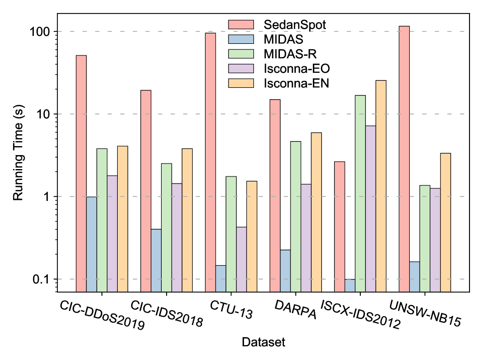
Figure 3: Time cost of Isconna and baselines

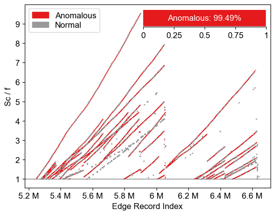
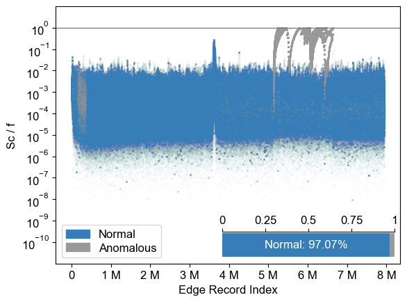
Figure 4: The contribution of pattern change detection to the final anomalousness measure, for final score greater than frequency score (left) and less than (right)

Fig. 4 shows the speed comparison of SedanSpot, MIDAS, MIDAS-R, Iscoona-EO, and Isconna-EN algorithms. F-Fade and PENminer are omitted since they are implemented in Python and spend minutes to hours processing large datasets (orders of magnitude slower). Note that on datasets other than ISCX-IDS2012, SedanSpot is significantly slower than other algorithms. On the other hand, MIDAS is the fastest among all algorithms. However, as seen in Table 3, this fast speed is at the cost of low detection accuracy.

Effectiveness of Pattern Detection

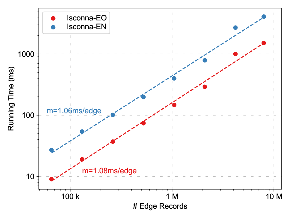
(a) For the number of edge records

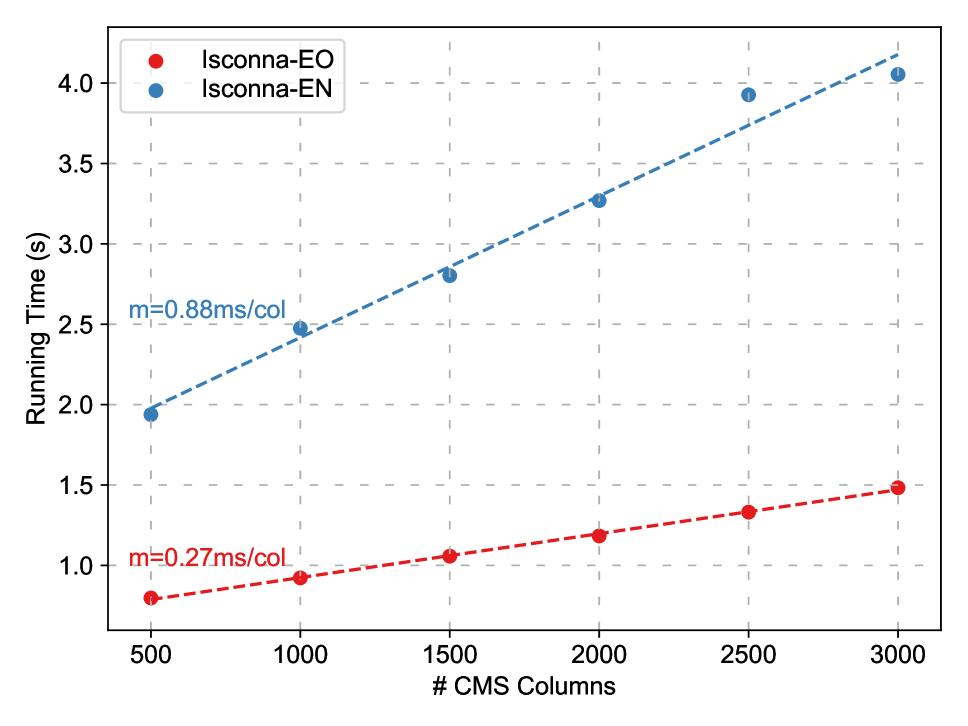
(b) For the number of CMS columns

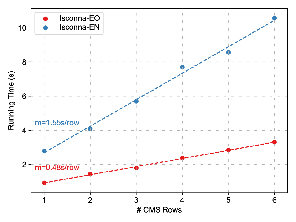
(c) For the number of CMS rows

Figure 5: Scalability (time cost vs. different parameter values)

In this part, we demonstrate the effectiveness of the pattern detection component by comparing the anomaly scores with and without width score and gap scores, i.e., comparing $A(e;\theta)$ and $B(e;\theta)$. We run Isconna-EO on the CIC-IDS2018 dataset. Fig. 4 (left) shows the edge records whose anomaly scores are increased after multiplying the pattern change score, i.e., $A(e;\theta)/B(e;\theta)>1$. Among them, 99.49% are true positive and 0.51% are false positive. This demonstrates that pattern detection can help better distinguish anomalous edge records by producing higher anomaly scores. On the other hand, Fig. 4 (right) shows edge records where $A(e;\theta)/B(e;\theta)<1$, of which 97.07% are true negative and 2.93% are false negative. This indicates that pattern detection is able to reduce the probability of incorrectly labeling normal edge records as anomalous, with an acceptable false negative rate.

Scalability

Fig. 5(a) shows the scalability of edge records. We test the required time to process the first $2^{16},2^{17},\dots,2^{22}$ and all edge records of the CIC-IDS2018 dataset. The results are spread around two lines, which indicates the running time of the algorithm on the whole dataset is linear to the number of edge records in it. Thus we can confirm the constant time complexity for processing individual edge records.

Fig. 5(b) and Fig. 5(c) show the CMS column scalability and the CMS row scalability, respectively. We can see the running time is linear to the number of columns/rows. This demonstrates that the size of CMSs is one of the terms of time complexity. Additionally, we may notice the slope of the EN variant is about three times of the EO variant. This is due to the extra CMSs for source nodes and destination nodes; both have a group of CMSs that resembles those of edges.

Conclusion

In this paper, we propose Isconna-EO and Isconna-EN algorithms, which detect burst and pattern anomalies in a streaming manner, without actively exploring or maintaining pattern snippets. The time complexity of processing an individual edge records is constant with respect to the data scale. Additionally, we provide a theoretical guarantee on the false positive probability. Our experimental results show that Isconna outperforms $5$ state-of-the-art frequency- or pattern-based baselines on $6$ real-world datasets, and demonstrate the scalability effectiveness of the pattern detection component. Future work could consider compatibility for general types of data and techniques for automatic parameter tuning.

References

- Abdelhamid et al. (2017) Abdelhamid, E.; Canim, M.; Sadoghi, M.; Bhattacharjee, B.; Chang, Y.; and Kalnis, P. 2017. Incremental Frequent Subgraph Mining on Large Evolving Graphs. IEEE Trans. Knowl. Data Eng., 29(12): 2710–2723.
- Akoglu, McGlohon, and Faloutsos (2010) Akoglu, L.; McGlohon, M.; and Faloutsos, C. 2010. oddball: Spotting Anomalies in Weighted Graphs. In Zaki, M. J.; Yu, J. X.; Ravindran, B.; and Pudi, V., eds., Advances in Knowledge Discovery and Data Mining, 14th Pacific-Asia Conference, PAKDD 2010, Hyderabad, India, June 21-24, 2010. Proceedings. Part II, volume 6119 of Lecture Notes in Computer Science, 410–421. Springer.
- Akoglu, Tong, and Koutra (2015) Akoglu, L.; Tong, H.; and Koutra, D. 2015. Graph based anomaly detection and description: a survey. Data Mining and Knowledge Discovery, 29(3): 626–688.
- Belth, Zheng, and Koutra (2020) Belth, C.; Zheng, X.; and Koutra, D. 2020. Mining Persistent Activity in Continually Evolving Networks. In Gupta, R.; Liu, Y.; Tang, J.; and Prakash, B. A., eds., KDD ’20: The 26th ACM SIGKDD Conference on Knowledge Discovery and Data Mining, Virtual Event, CA, USA, August 23-27, 2020, 934–944. ACM.
- Beutel et al. (2013) Beutel, A.; Xu, W.; Guruswami, V.; Palow, C.; and Faloutsos, C. 2013. CopyCatch: stopping group attacks by spotting lockstep behavior in social networks. In Schwabe, D.; Almeida, V. A. F.; Glaser, H.; Baeza-Yates, R.; and Moon, S. B., eds., 22nd International World Wide Web Conference, WWW ’13, Rio de Janeiro, Brazil, May 13-17, 2013, 119–130. International World Wide Web Conferences Steering Committee / ACM.
- Bhatia et al. (2020) Bhatia, S.; Hooi, B.; Yoon, M.; Shin, K.; and Faloutsos, C. 2020. Midas: Microcluster-Based Detector of Anomalies in Edge Streams. In The Thirty-Fourth AAAI Conference on Artificial Intelligence, AAAI 2020, The Thirty-Second Innovative Applications of Artificial Intelligence Conference, IAAI 2020, The Tenth AAAI Symposium on Educational Advances in Artificial Intelligence, EAAI 2020, New York, NY, USA, February 7-12, 2020, 3242–3249. AAAI Press.
- Chakrabarti (2004) Chakrabarti, D. 2004. AutoPart: Parameter-Free Graph Partitioning and Outlier Detection. In Boulicaut, J.; Esposito, F.; Giannotti, F.; and Pedreschi, D., eds., Knowledge Discovery in Databases: PKDD 2004, 8th European Conference on Principles and Practice of Knowledge Discovery in Databases, Pisa, Italy, September 20-24, 2004, Proceedings, volume 3202 of Lecture Notes in Computer Science, 112–124. Springer.
- Chalapathy and Chawla (2019) Chalapathy, R.; and Chawla, S. 2019. Deep Learning for Anomaly Detection: A Survey.
- Chandola, Banerjee, and Kumar (2009) Chandola, V.; Banerjee, A.; and Kumar, V. 2009. Anomaly detection. ACM Computing Surveys, 41(3): 1–58.
- Chang et al. (2021) Chang, Y.; Li, P.; Sosic, R.; Afifi, M. H.; Schweighauser, M.; and Leskovec, J. 2021. F-FADE: Frequency Factorization for Anomaly Detection in Edge Streams. In Lewin-Eytan, L.; Carmel, D.; Yom-Tov, E.; Agichtein, E.; and Gabrilovich, E., eds., WSDM ’21, The Fourteenth ACM International Conference on Web Search and Data Mining, Virtual Event, Israel, March 8-12, 2021, 589–597. ACM.
- Cormode and Muthukrishnan (2004) Cormode, G.; and Muthukrishnan, S. 2004. An Improved Data Stream Summary: The Count-Min Sketch and Its Applications. In Farach-Colton, M., ed., LATIN 2004: Theoretical Informatics, 6th Latin American Symposium, Buenos Aires, Argentina, April 5-8, 2004, Proceedings, volume 2976 of Lecture Notes in Computer Science, 29–38. Springer.
- Cressie and Read (1984) Cressie, N.; and Read, T. R. 1984. Multinomial Goodness-Of-Fit Tests. Journal of the Royal Statistical Society: Series B (Methodological), 46(3): 440–464.
- Eswaran and Faloutsos (2018) Eswaran, D.; and Faloutsos, C. 2018. SedanSpot: Detecting Anomalies in Edge Streams. In IEEE International Conference on Data Mining, ICDM 2018, Singapore, November 17-20, 2018, 953–958. IEEE Computer Society.
- Eswaran et al. (2018) Eswaran, D.; Faloutsos, C.; Guha, S.; and Mishra, N. 2018. SpotLight: Detecting Anomalies in Streaming Graphs. In Guo, Y.; and Farooq, F., eds., Proceedings of the 24th ACM SIGKDD International Conference on Knowledge Discovery & Data Mining, KDD 2018, London, UK, August 19-23, 2018, 1378–1386. ACM.
- García et al. (2014) García, S.; Grill, M.; Stiborek, J.; and Zunino, A. 2014. An empirical comparison of botnet detection methods. Comput. Secur., 45: 100–123.
- Hooi et al. (2017) Hooi, B.; Shin, K.; Song, H. A.; Beutel, A.; Shah, N.; and Faloutsos, C. 2017. Graph-Based Fraud Detection in the Face of Camouflage. ACM Trans. Knowl. Discov. Data, 11(4): 44:1–44:26.
- Jiang et al. (2016) Jiang, M.; Cui, P.; Beutel, A.; Faloutsos, C.; and Yang, S. 2016. Catching Synchronized Behaviors in Large Networks: A Graph Mining Approach. ACM Trans. Knowl. Discov. Data, 10(4): 35:1–35:27.
- Kleinberg (1999) Kleinberg, J. M. 1999. Authoritative Sources in a Hyperlinked Environment. J. ACM, 46(5): 604–632.
- Lippmann et al. (1999) Lippmann, R.; Cunningham, R. K.; Fried, D. J.; Graf, I.; Kendall, K. R.; Webster, S. E.; and Zissman, M. A. 1999. Results of the DARPA 1998 Offline Intrusion Detection Evaluation. In Recent Advances in Intrusion Detection, Second International Workshop, RAID 1999, West Lafayette, Indiana, USA, September 7-9, 1999.
- Moustafa and Slay (2015) Moustafa, N.; and Slay, J. 2015. UNSW-NB15: a comprehensive data set for network intrusion detection systems (UNSW-NB15 network data set). In 2015 Military Communications and Information Systems Conference, MilCIS 2015, Canberra, Australia, November 10-12, 2015, 1–6. IEEE.
- Page et al. (1999) Page, L.; Brin, S.; Motwani, R.; and Winograd, T. 1999. The PageRank Citation Ranking: Bringing Order to the Web. Technical Report 1999-66. Previous number = SIDL-WP-1999-0120.
- Ranshous et al. (2016) Ranshous, S.; Harenberg, S.; Sharma, K.; and Samatova, N. F. 2016. A Scalable Approach for Outlier Detection in Edge Streams Using Sketch-based Approximations. In Venkatasubramanian, S. C.; and Jr., W. M., eds., Proceedings of the 2016 SIAM International Conference on Data Mining, Miami, Florida, USA, May 5-7, 2016, 189–197. SIAM.
- Sharafaldin, Lashkari, and Ghorbani (2018) Sharafaldin, I.; Lashkari, A. H.; and Ghorbani, A. A. 2018. Toward Generating a New Intrusion Detection Dataset and Intrusion Traffic Characterization. In Mori, P.; Furnell, S.; and Camp, O., eds., Proceedings of the 4th International Conference on Information Systems Security and Privacy, ICISSP 2018, Funchal, Madeira - Portugal, January 22-24, 2018, 108–116. SciTePress.
- Sharafaldin et al. (2019) Sharafaldin, I.; Lashkari, A. H.; Hakak, S.; and Ghorbani, A. A. 2019. Developing Realistic Distributed Denial of Service (DDoS) Attack Dataset and Taxonomy. In 2019 International Carnahan Conference on Security Technology (ICCST). IEEE.
- Shin, Eliassi-Rad, and Faloutsos (2018) Shin, K.; Eliassi-Rad, T.; and Faloutsos, C. 2018. Patterns and anomalies in k-cores of real-world graphs with applications. Knowl. Inf. Syst., 54(3): 677–710.
- Shin et al. (2017) Shin, K.; Hooi, B.; Kim, J.; and Faloutsos, C. 2017. DenseAlert: Incremental Dense-Subtensor Detection in Tensor Streams. In Proceedings of the 23rd ACM SIGKDD International Conference on Knowledge Discovery and Data Mining, Halifax, NS, Canada, August 13 - 17, 2017, 1057–1066. ACM.
- Shiravi et al. (2012) Shiravi, A.; Shiravi, H.; Tavallaee, M.; and Ghorbani, A. A. 2012. Toward developing a systematic approach to generate benchmark datasets for intrusion detection. Comput. Secur., 31(3): 357–374.
- Siffer et al. (2017) Siffer, A.; Fouque, P.; Termier, A.; and Largouët, C. 2017. Anomaly Detection in Streams with Extreme Value Theory. In Proceedings of the 23rd ACM SIGKDD International Conference on Knowledge Discovery and Data Mining, Halifax, NS, Canada, August 13 - 17, 2017, 1067–1075. ACM.
- Sricharan and Das (2014) Sricharan, K.; and Das, K. 2014. Localizing anomalous changes in time-evolving graphs. In Dyreson, C. E.; Li, F.; and Özsu, M. T., eds., International Conference on Management of Data, SIGMOD 2014, Snowbird, UT, USA, June 22-27, 2014, 1347–1358. ACM.
- Sun, Tao, and Faloutsos (2006) Sun, J.; Tao, D.; and Faloutsos, C. 2006. Beyond streams and graphs: dynamic tensor analysis. In Eliassi-Rad, T.; Ungar, L. H.; Craven, M.; and Gunopulos, D., eds., Proceedings of the Twelfth ACM SIGKDD International Conference on Knowledge Discovery and Data Mining, Philadelphia, PA, USA, August 20-23, 2006, 374–383. ACM.
- Tong and Lin (2011) Tong, H.; and Lin, C. 2011. Non-Negative Residual Matrix Factorization with Application to Graph Anomaly Detection. In Proceedings of the Eleventh SIAM International Conference on Data Mining, SDM 2011, April 28-30, 2011, Mesa, Arizona, USA, 143–153. SIAM / Omnipress.
- Yoon et al. (2019) Yoon, M.; Hooi, B.; Shin, K.; and Faloutsos, C. 2019. Fast and Accurate Anomaly Detection in Dynamic Graphs with a Two-Pronged Approach. In Teredesai, A.; Kumar, V.; Li, Y.; Rosales, R.; Terzi, E.; and Karypis, G., eds., Proceedings of the 25th ACM SIGKDD International Conference on Knowledge Discovery & Data Mining, KDD 2019, Anchorage, AK, USA, August 4-8, 2019, 647–657. ACM.
- Yu et al. (2013) Yu, W.; Aggarwal, C. C.; Ma, S.; and Wang, H. 2013. On Anomalous Hotspot Discovery in Graph Streams. In Xiong, H.; Karypis, G.; Thuraisingham, B. M.; Cook, D. J.; and Wu, X., eds., 2013 IEEE 13th International Conference on Data Mining, Dallas, TX, USA, December 7-10, 2013, 1271–1276. IEEE Computer Society.