Reinforcement Learning with Temporal Logic Constraints for Partially-Observable Markov Decision Processes

Abstract

This paper proposes a reinforcement learning method for controller synthesis of autonomous systems in unknown and partially-observable environments with subjective time-dependent safety constraints. Mathematically, we model the system dynamics by a partially-observable Markov decision process (POMDP) with unknown transition/observation probabilities. The time-dependent safety constraint is captured by iLTL, a variation of linear temporal logic for state distributions. Our Reinforcement learning method first constructs the belief MDP of the POMDP, capturing the time evolution of estimated state distributions. Then, by building the product belief MDP of the belief MDP and the limiting deterministic Büchi automaton (LDBA) of the temporal logic constraint, we transform the time-dependent safety constraint on the POMDP into a state-dependent constraint on the product belief MDP. Finally, we learn the optimal policy by value iteration under the state-dependent constraint.

I Introduction

Reinforcement learning methods are widely used to synthesize control policies for autonomous systems that work in unknown environments (e.g., robotics and unmanned vehicles) [1]. Among them, model-free reinforcement learning methods are of particular interest since they can derive control policies without identifying the complete system model [1]. Instead, they can find the best control policy for a given discounted reward function by iteratively rolling out a tentative control policy and improving it based on observed system behaviors. For systems with fully observable states, algorithms have been developed for various tasks [2, 3, 4] including linear temporal logic tasks [5, 6, 7, 8, 9].

More often than not, the states of real-world autonomous systems such as self-driving cars [10] and robots [11] are not fully observable due to system/environment uncertainty (e.g., sensor noise). For these applications, a widely-used mathematical model for control synthesis is the partially observable Markov decision process (POMDP) [12]. A POMDP generalizes a Markov decision process (MDP), whose states are partially-observable through a probabilistic relation to a set of observations. Due to the partial observability, control synthesis is considerably harder for POMDP than fully observable models like Markov decision processes. Most of the exact decision problems on POMDP are either undecidable or PSPACE-complete [13, 14].

This work studies the control synthesis for POMDPs in the Bayesian framework. Instead of exhaustively consider all states agreeing with the observation (e.g., in [13, 14]), we based the control actions on the posterior state estimation, i.e., beliefs. For a given observation, the evolution of beliefs under the control actions is captured by a Markov decision process with infinitely many states. Thus, the Bayesian framework “lifts” the POMDP control problem into a (fully-observable) MDP control problem at the cost of expanding the state space. Accordingly, we value iteration methods to deal with the infinite product belief space [15, 16].

A crucial concern in learning-based control synthesis is dynamical safety. For safety-critical systems, such as self-driving cars [10] and robots [11], designing a policy that guarantees both safety and optimality is necessary. Typically, the safety constraints are time-dependent and expressible by linear temporal logic (LTL), a set of symbols and rules for formally representing and reasoning about time-dependent properties [17]. For different scenarios, variations of LTL in syntax and semantics are used [18].

This work considers safety constraints expressed by iLTL, a variation of LTL for state distributions. It has found applications in wireless sensor network [19] and cyber-physical systems [20, 21]. Compare to barrier certificates [22], iLTL is more expressive for time-dependent safety constraints. We use iLTL to capture safety constraints for posterior state estimations (i.e., beliefs) of the POMDP. Namely, when synthesizing the optimal control for a given discounted reward, if we “believe” an action will violate the iLTL safety constraint, we should not take it.

We propose a reinforcement learning method to derive the optimal control policy for a given discounted reward under an iLTL safety constraint. By constructing the belief MDP of the POMDP, we first lift the control synthesis problem to the belief space. Then, we build the product belief MDP of the belief MDP and the limiting deterministic Büchi automaton (LDBA) of the temporal logic constraint. This transforms the time-dependent iLTL constraint to a state-dependent Büchi constraint on the product belief MDP [8]. Finally, we propose a value iteration method to learn the optimal policy for the discounted reward under the Büchi constraint. An overview of our approach is shown by Figure 1.

The rest of the paper runs as follows. We give the definition of POMDP in Section II and formula the control synthesis problem Section III. We introduce the LDBA and build the product belief MDP in Section IV. Then, we introduce the value iteration under constraints and the learning algorithm in Section V. Finally, we conclude this work in Section VI.

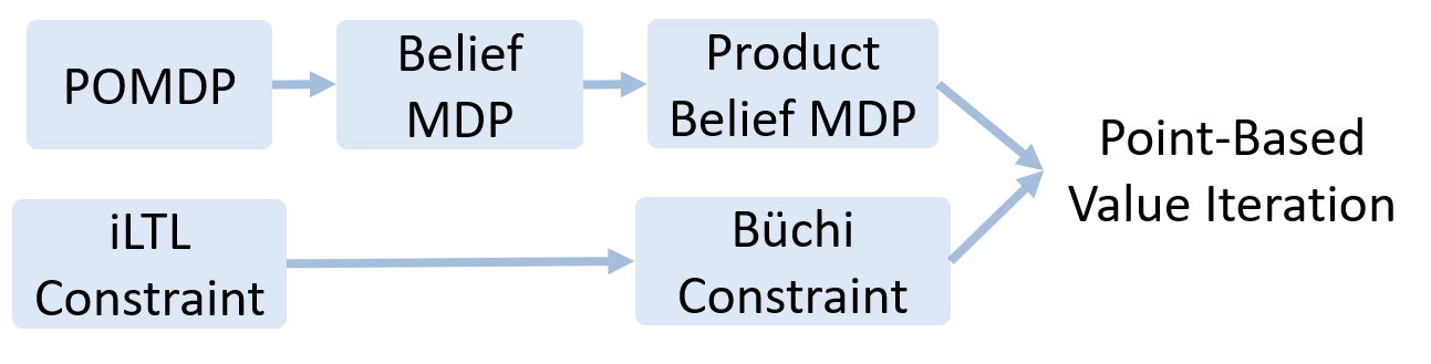
Figure 1: An overview of our method.

II Preliminaries

We model an autonomous system’s dynamics in the unknown and partially-observable environment by a partially-observable Markov decision process (POMDP), where the underline dynamics is a Markov decision process, but the control can only depend on observations probabilistically related to the states.

For a finite $S$, we denote the set of probability distributions on $S$ by $\text{Dist}(S)$. A POMDP is a tuple $\mathcal{M}=(S,A,T,p_{0},r,\gamma,O,\Omega)$, where

• $S=\{s_{1},\ldots,s_{n}\}$ is a set of $n$ states.

• $A=\{a_{1},\ldots,a_{m}\}$ is a set of $m$ actions.

• $T:S\times A\times S\to[0,1]$ is a set of transition probabilities between states, satisfying for any $s\in S$ and any $a\in A$,

  $$\sum_{s^{\prime}\in S}T(s,a,s^{\prime})=1.$$

  By taking the action $a\in A$ on the state $s\in S$, the probability of transiting to the state $s^{\prime}\in S$ is $T(s,a,s^{\prime})$.

• $p_{0}\in\text{Dist}(S)$ is an initial distribution.

• $r:S\to\real$ is the immediate reward function.

• $\gamma:S\to(0,1)$ is a discount factor.

• $O=\{o_{1},\ldots,o_{l}\}$ is a set of $l$ observations.

• $\Omega:S\times O$ is a set of observation probabilities, satisfying for any $s\in S$

  $$\sum_{o\in O}\Omega(s,o)=1.$$

  On the state $s$, the probability of yielding an observation $o$ is $\Omega(s,o)$.

When $S=O$ and $\Omega(s,o)=1$ if and only if $s=o$, the POMDP $\mathcal{M}$ reduces to a Markov decision process (MDP). We call a sequence of states $\sigma:\mathbb{N}\to S$ a path of the POMDP if for any $t\in\mathbb{N}$, there exists $a\in A$ such that $T(s(t),a,s(t+1))>0$. In addition, we call a sequences of state distributions $\sigma:\mathbb{N}\to\text{Dist}(S)$ as an execution of the POMDP.

III Problem Formulation

We consider the control synthesis problem on the POMDP from Section II. Mathematically, the control policy

$$\pi:O^{*}\to\text{Dist}(A)$$ (1)

decides (probabilistically) the action to take from the history of observations. We denote the POMDP under the control policy by $\mathcal{M}_{\pi}$ and a random path drawn from the controlled POMDP by $\sigma\sim\mathcal{M}_{\pi}$. The control goal is to maximize the expected cumulative reward of the random path $\sigma$; equivalently, we look for the optimal control policy $\pi^{*}$ such that

$$\pi^{*}=\mathrm{argmax}_{\pi}\mathbb{E}_{\sigma\sim\mathcal{M}_{\pi}}R(\sigma),$$ (2)

where

$$R(\sigma)=\sum_{i=1}^{\infty}\gamma^{t}r(\sigma(t)).$$ (3)

III-A Belief Markov Decision Processes

The states are not directly observable in a POMDP. But, from a history of observation, one can derive a probabilistic estimation of the states from the history of observations is called a belief $b\in\text{Dist}(S)$. At $t=0$, the belief $b_{0}$ is the initial distribution, i.e., $b_{0}=p_{0}$. For $t>0$, the belief $b_{t}$ updates upon observing $o$ by the Bayes rule

$$\begin{split}b_{t+1}(s^{\prime})=\frac{\Omega(s^{\prime},o)\sum_{s\in S}T(s,a,s^{\prime})b_{t}(s)}{\sum_{s^{\prime}\in S}\Omega(s^{\prime},o)\sum_{s\in S}T(s,a,s^{\prime})b_{t}(s)}\end{split}$$ (4)

Following (4), the POMDP $\mathcal{M}$ induces a Markov decision process (MDP) on the belief space $\text{Dist}(S)$ where each belief (i.e., state distribution) is a state. It shows how the belief changes for taking different actions. The belief MDP is fully observable.

Definition 1.

The belief MDP $\mathcal{D}$ of the POMDP $\mathcal{M}\allowbreak=(S,A,T,p_{0},r,\gamma,O,\Omega)$ is defined by $\mathcal{D}=(\text{Dist}(S),\allowbreak A,T_{\mathcal{D}},p_{0},r_{\mathcal{D}},\gamma)$ where

$$T_{\mathcal{D}}(b,a,b^{\prime})=\sum_{o\in O}\sum_{s^{\prime}\in S}\sum_{s\in S}\eta(b,o,b^{\prime})\Omega(s^{\prime},o)T(s,a,s^{\prime})b(s)$$

with

$$\begin{split}&\eta(b,o,b^{\prime})\\ &=\bigg{\{}\begin{array}[]{ll}1,&\text{if the belief update for }b,o\text{ by~{}\eqref{eq:belief update} returns }b^{\prime},\\ 0,&\text{otherwise,}\end{array}\end{split}$$

and

$$r_{\mathcal{D}}(b,a)=\sum_{s\in S}b(s)r(s,a)$$

for $b,b^{\prime}\in\text{Dist}(S)$ and $a\in A$.

III-B Time-Dependent Safety Constraints

We formally capture time-dependent safety constraints by temporal logic. For the probabilistic safety related to state distributions, we introduce a variant of the linear temporal logic (LTL) to capture time-dependent specifications for wireless sensor network [19] and cyber-physical systems [20, 21].

An inequality LTL (iLTL) formula is derived recursively from the rules

$$\varphi\Coloneqq f\mid\neg\varphi\mid\varphi\land\varphi\mid\bigcirc\varphi\mid\varphi\mathbin{\mathcal{U}}_{T}\varphi$$ (5)

where

• $f:{}^{n}\to\real$ is a (given) function and is called an atomic proposition.

• $T\in\mathbb{N}$ and $\bigcirc$ and $\mathbin{\mathcal{U}}$ are temporal operators, meaning “next” and “until”, respectively.

Other common logic operators can be derived as follows: $\text{True}\equiv\varphi\land\neg\varphi$, $\varphi\land\varphi^{\prime}\equiv\neg(\neg\varphi\wedge\neg\varphi^{\prime})$, $\varphi\rightarrow\varphi^{\prime}\equiv\neg\varphi\land\varphi^{\prime}$, $\Diamond_{T}\varphi\equiv\text{True}U_{T}\varphi$, and $\Box_{T}\varphi\equiv\neg\Diamond_{T}\neg\varphi$. Also, we denote $\mathbin{\mathcal{U}}_{T},\Diamond_{T},$ and $\Box_{T}$ by $\mathbin{\mathcal{U}},\Diamond$ and $\Box$, respectively. Our definition of iLTL is more general than [19, 20, 21], since we allow atomic proposition $f$ in (5) to be nonlinear functions.

Let $\sigma:\mathbb{N}\to\text{Dist}(S)$ be a execution of the POMDP. The satisfaction (denoted by $\models$) of an iLTL formula is defined recursively by the rules

$$\sigma\models f\text{ iff }f(\sigma(0))>0$$

$$\sigma\models\neg\varphi\text{ iff }\sigma\not\models\varphi$$

$$\sigma\models\varphi_{1}\land\varphi_{2}\text{ iff }\sigma\models\psi_{1}\text{ and }\sigma\models\varphi_{2}$$

$$\sigma\models\bigcirc\varphi\text{ iff }\sigma^{[1]}\models\varphi$$

$$\sigma\models\varphi_{1}\mathbin{\mathcal{U}}_{T}\varphi_{2}\text{ iff }\exists t\leq T.\big{(}\sigma^{[t]}\models\varphi\text{ and }\forall t^{\prime}\leq t.\ \sigma^{[t^{\prime}]}\models\varphi\big{)}$$

where $\sigma^{[t]}$ is the $t$-shift of $\sigma$ defined by $\sigma^{[t]}(t^{\prime})=\sigma(t+t^{\prime})$ for any $t^{\prime}\in\mathbb{N}$.

Using iLTL, we can express a wide class of time-dependent safety properties. For example, consider a general probabilistic space $S$. Let $S_{1},S_{2}\subseteq S$ and $I_{S_{1}}$ and $I_{S_{2}}$ be the indicator functions, respectively. Then the iLTL formula

$$\varphi=\Diamond\Box(0.1-I_{S_{1}})\lor\Diamond\Box(I_{S_{2}}-0.8)$$ (6)

means that the probability of finally always staying in the (unsafe) set $S_{1}$ should be less than $0.1$ and the probability of finally always staying the (goal) set $S_{2}$ should be great than $0.8$.

III-C Control Synthesis Under iLTL Constraints

Based on modeling the system by a POMDP and the time-dependent safety constraint by iLTL, we formally introduce the problem formulation below.

Problem 1.

Given the MDP from Section II and the iLTL constraint $\varphi$ from Section III-B, find a policy $\pi$ in the form of (1) maximize the expected value of the discounted reward (3), while ensuring the belief sequence $b_{0}b_{1}\ldots$ derived from (4) satisfies $\varphi$.

In Problem 1, the constraint $b_{0}b_{1}\ldots\models\varphi$ means when synthesizing the optimal control for a given discounted reward, if we “believe” an action will violate the iLTL safety constraint, we should not take it. Besides, in our Bayesian framework discussed in Section III-A, the control policy $\pi:O^{*}\to\text{Dist}(A)$ depends on past observations through belief updates (which are a sufficient statistic). Thus, to maximize the discounted reward (3) (without the safety constraint $\varphi$), we only need the belief sequence $b_{0}b_{1}\ldots$. In addition, since the satisfaction of the safety constraint $\varphi$ also involves the belief sequence $b_{0}b_{1}\ldots$, it suffices to consider a policy mapping belief sequences to actions. This is summarized by the following lemma.

Lemma 1.

To solve Problem 1, it suffices to find a policy

$$\pi:\text{Dist}(S)^{*}\to A.$$ (7)

IV Product Belief MDP

Following Lemma 1, the control policy that solves Problem 1 depends on the past belief sequence, so is memory-dependent; this is beyond the capability of reinforcement learning. To remove the memory dependency, we generalize the product technique from [8] to belief MDPs that have infinite states.

IV-A Limiting-Deterministic Büchi Automata

An LDBA is a tuple $\mathcal{A}=(Q,\Sigma,\delta,q_{0},B)$ where

• $Q$ is a finite set of states;

• $\Sigma$ is a finite set of alphabets;

• $\delta:Q\times(\Sigma\cup\{\varepsilon\})\to Q$ is a (partial) transition function (i.e., all alphabets are allowed on each state) with $\varepsilon$ standing for the empty alphabet.

• $q_{0}\in Q$ is an initial state;

• $B$ is a set of accepting states.

The LDBA satisfies that

• the transition $\delta$ is total except for the empty alphabet, i.e., $|\delta(q,\cdot)|=1$ for any $q\in Q$;

• there exists a bipartition of into an initial and accepting component, i.e., $Q=Q_{A}\cup Q_{I}$ such that

  • transitions from the accepting component stay within it, i.e., $\delta(q,\cdot)\subseteq Q_{A}$ for any $q\in Q_{A}$;

  • the accepting states are in the accepting component, i.e., $B\subseteq Q_{A}$.

  • the $\varepsilon$-moves are not allowed in the accepting component, i.e., $\delta(q,\varepsilon)=\emptyset$ for any $q\in Q_{A}$;

We call $q:\mathbb{N}\to Q$ a path of the LDBA if $q(0)=q_{0}$ and for any $t\in\mathbb{N}$, there exists $\sigma\in\Sigma$ such that $q(t+1)=\delta(q(t),\sigma)$. The path $q$ is accepted if $\text{Inf}(q)\cup B\neq\emptyset$, i.e., some state in $B$ appears infinitely often in $q$. Accordingly, an alphabet sequence is accepted if there exists a corresponding accepted path. As a variation of the standard linear temporal logic (LTL), an iLTL formula yields a graphic representation called a limiting-deterministic Büchi automaton (LDBA) [24, 8].

Lemma 2.

For any iLTL formula $\varphi$, there exists an LDBA $\mathcal{A}$ (whose alphabets are sets of iLTL atomic propositions from (5)) such that a sequence $b\models\varphi$ if and only if $b$ is accepted by $\mathcal{A}$. Accordingly, we call $\mathcal{A}$ realizes $\varphi$.

For example, an LDBA realizing the iLTL formula (6) is shown by Figure 2.

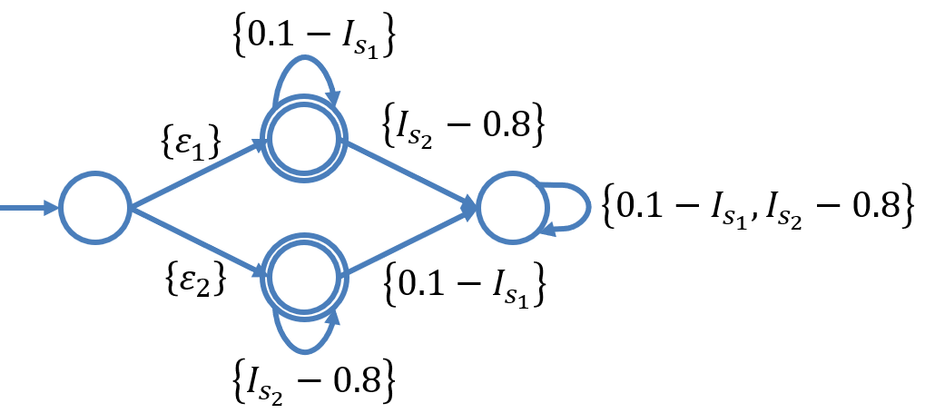
Figure 2: The figure shows an LDBA for the iLTL formula (6). We index the empty alphabets $\varepsilon_{1}$ and $\varepsilon_{2}$ to distinguish. The accepting states are double circled.

IV-B Product Belief MDP

Definition 2.

The product belief MDP $\mathcal{D}^{\times}=\mathcal{D}\times\mathcal{A}$ of the belief MDP $\mathcal{D}=(\text{Dist}(S),A,T_{\mathcal{D}},p_{0},\allowbreak r_{\mathcal{D}},\gamma)$ and an LDBA $\mathcal{A}=(Q,\Sigma,\delta,q_{0},B)$ is defined by $\mathcal{D}^{\times}=(\text{Dist}(S)\times Q,A\cup\{\varepsilon\},T^{\times},(p_{0},q_{0}),r^{\times},\gamma)$ where

$$T^{\times}\big{(}(b,q),a,(b^{\prime},q^{\prime})\big{)}=$$

$$\qquad\begin{cases}T_{\mathcal{D}}(b,a,b^{\prime})&\text{if }a\in A,q^{\prime}=\delta(q,L(b))\\ 1&\text{if }a=\varepsilon,q^{\prime}\in\delta(q,\varepsilon),b=b^{\prime}\\ 0&\text{otherwise}\end{cases}$$ (8)

$$L(b)=\{f\text{ is an atomic proposition in }\varphi\mid f(b)>0\}$$ (9)

and

$$r^{\times}\big{(}(b,q)\big{)}=r_{\mathcal{D}}(b).$$ (10)

In addition, let

$$B^{\times}=\{(b,q)\in\text{Dist}(S)\times Q\mid q\in B\}.$$ (11)

A path $(b_{0},q_{0})(b_{1},q_{1})\ldots$ of the product belief MDP corresponds uniquely to the combination of a path $b_{0}b_{1}\ldots$ of the belief MDP and a path $q_{0}q_{1}\ldots$ of the LDBA; and vice versa. Following (11), the path $q_{0}q_{1}\ldots$ is accepted by the LDBA (i.e., some states in $B$ appears in it infinitely often) if and only if some states in $B^{\times}$ appear infinitely often in the product path $(b_{0},q_{0})(b_{1},q_{1})\ldots$. Also, the reward (10) for the path $(b_{0},q_{0})(b_{1},q_{1})\ldots$ is equal to the reward (3) for the path $(b_{0},q_{0})(b_{1},q_{1})\ldots$. The existence of $\varepsilon$ moves in the LDBA (and the $\varepsilon$ actions in the product belief MDP) does not affect the path correspondence. Thus, we can reduce the iLTL constraint on the belief MDP to a Büchi constraint (i.e., visiting certain states infinitely often) on the product belief MDP, as stated by the following lemma.

Theorem 1.

If $\mathcal{D}^{\times}=\mathcal{D}\times\mathcal{A}$, then

$$\max_{\pi}\mathbb{P}_{\sigma\sim\mathcal{D}_{\pi}}(\sigma\models\varphi)=\max_{\pi^{\times}}\mathbb{P}_{\sigma^{\times}\sim\mathcal{D}^{\times}_{\pi^{\times}}}(\sigma^{\times}\models\Box\Diamond B^{\times}\big{)}$$ (12)

and

$$\max_{\pi}\mathbb{E}_{\sigma\sim\mathcal{D}_{\pi}}(\sum_{i=1}^{\infty}\gamma^{t}r(\sigma(t)))$$

$$\qquad=\max_{\pi^{\times}}\mathbb{E}_{\sigma^{\times}\sim\mathcal{D}^{\times}_{\pi^{\times}}}(\sum_{i=1}^{\infty}\gamma^{t}r^{\times}(\sigma^{\times}(t))),$$ (13)

where $\pi$ is of the form (7); and similarly $\pi^{\times}$.

Proof.

Follow from the proof Theorem 1 in [8], noting that $L(b)$ in (9) contains all atomic propositions holds on the (belief) state $b$. ∎

Furthermore, the maxima of the right-hand side of (12) and (1) can be memoryless. Despite the existence of $\varepsilon$ actions, this memoryless policy maps to a memory-dependent policy on the belief MDP, which maximizes the left-hand side of (12) and (1), as formally stated below.

Corollary 1.

A memoryless policy maximizes the right-hand side of (12) and (1). It induces a memory-dependent policy that maximizes the left-hand side of (12) and (1).

Proof.

Follow from the proof Theorem 3 in [24]. ∎

V Learning under Constraints

The product belief MDP has an infinite states space $\text{Dist}(S)\times Q$. Thus the tabular reinforcement learning method does not apply. Here, we generalize the value iteration method [25, 15] to solve for the optimal control policy under the constraint.

V-A Bellman Equation on Belief Space

We define the value function for the reward $r^{\times}$ on the product belief space by

$$V_{r}\big{(}(b,q)\big{)}=\max_{\pi^{\times}}\mathbb{E}_{\sigma^{\times}\sim\mathcal{D}^{\times}_{\pi^{\times},(b,q)}}\sum_{t\in\mathbb{N}}\gamma^{t}r^{\times}(\sigma(t))$$ (14)

where $\sigma^{\times}\sim\mathcal{D}^{\times}_{\pi^{\times},(b,q)}$ is a random path drawn from $\mathcal{D}^{\times}$ under the policy $\pi$ from the product state $(b,q)$. The value function $V_{r}$ captures the maximal expected value of the reward (3) if started from the product state $(b,q)$. By Theorem 1, $V_{r}(p_{0},q_{0})$ is the maximal expected reward of (3) on the POMDP $\mathcal{M}$.

In addition, we define the value function for the Büchi constraint on the product belief space by

$$V_{p}\big{(}(b,q)\big{)}=\max_{\pi^{\times}}\mathbb{P}_{\sigma\sim\mathcal{D}^{\times}_{\pi^{\times},(b,q)}}\big{(}\sigma\models\Box\Diamond B^{\times}\big{)}$$ (15)

The value function $V_{p}$ captures the maximal satisfaction probability of the Büchi constraint $\Box\Diamond B^{\times}$ if started from the product state $(b,q)$. By Theorem 1, $V_{p}(p_{0},q_{0})$ is the maximal satisfaction probability of the iLTL safety constraint $\varphi$ on the POMDP $\mathcal{M}$.

From Corollary 1, it suffices to consider pure and memoryless policy to maximize the two wo values functions (14) and (15). Accordingly, they satisfy the following Bellman equations

$$V_{r}\big{(}(b,q)\big{)}=\max_{a\in A}Q_{r}\big{(}(b,q),a\big{)}$$ (16)

$$Q_{r}\big{(}(b,q),a\big{)}=r^{\times}\big{(}(b,q)\big{)}+\gamma\sum_{q^{\prime}\in Q}\int_{b^{\prime}\in\text{Dist}(S)}$$

$$\qquad T^{\times}\Big{(}\big{(}(b,q)\big{)},a,\big{(}(b^{\prime},q^{\prime})\big{)}\Big{)}V_{r}\big{(}(b^{\prime},q^{\prime})\big{)}\mathrm{d}b^{\prime}$$ (17)

and

$$V_{p}\big{(}(b,q)\big{)}=\max_{a\in A}Q_{p}\big{(}(b,q),a\big{)}$$

$$Q_{p}\big{(}(b,q),a\big{)}=\sum_{q^{\prime}\in Q}\int_{b^{\prime}\in\text{Dist}(S)}$$

$$\qquad T^{\times}\Big{(}\big{(}(b,q)\big{)},a,\big{(}(b^{\prime},q^{\prime})\big{)}\Big{)}V_{p}\big{(}(b^{\prime},q^{\prime})\big{)}\mathrm{d}b^{\prime}$$ (18)

For solving (V-A), we also have

$$V_{p}\big{(}(b,q)\big{)}=1\text{ for }(b,q)\in B^{\times}$$ (19)

where $B^{\times}$ is given by (11), according to iLTL syntax.

V-B Value Iteration

Our learning method aims to find solutions to the Bellman equations (17) and (V-A) by sampling, without using knowledge on the transition probabilities $T^{\times}$. Since the product belief space $\text{Dist}(S)\times Q$ is infinite, tabular learning methods are not applicable. Instead, we generalize the value iteration method [25] to the product belief space. Our method is based on the fact that the value functions and Q-functions are piecewise linear, as stated below.

Lemma 3.

The value functions $V_{r}\big{(}(b,q)\big{)}$ and $V_{p}\big{(}(b,q)\big{)}$ and Q-functions $Q_{r}\big{(}(b,q),a\big{)}$ and $Q_{p}\big{(}(b,q),a\big{)}$ are convex and piecewise linear in $b$.

Proof.

It suffices to prove the statement for each $q\in Q$, which follows directly from [25]. ∎

Based on Lemma 3, we can represent the Q-function $Q_{r}$ (and the same for $Q_{p}$) on the product space by

$$Q_{r}\big{(}(b,q),a\big{)}=\max_{\theta\in\Theta_{q,a}}\sum_{s\in S}\theta(s)b(s)$$ (20)

$$V_{r}\big{(}(b,q)\big{)}=\max_{\theta\in\Theta_{q}}\sum_{s\in S}\theta(s)b(s)$$ (21)

where each $\Theta_{q}$ and $\Theta_{q,a}$ (for $q\in Q$ and $a\in A$) is a finite set of $|S|$-dimensional vectors, which define hyperplanes on the belief space. Following (16), we can take

$$\Theta_{q}=\cup_{a\in A}\Theta_{q,a}.$$ (22)

Our goal is to identify the set $\Theta_{q,a}$ (thus $\Theta_{q}$). By plugging (20)-(22) into the the Bellman equation (17) and using Definition 2, we have

$$Q_{r}\big{(}(b,q),a\big{)}= \sum_{s\in S}r(s)b(s)+\gamma\int_{b^{\prime}\in\text{Dist}(S)}$$

$$T_{\mathcal{D}}(b,a,b^{\prime})\max_{\theta\in\Theta_{q^{\prime}}}\sum_{s\in S}\theta(s)b^{\prime}(s)\mathrm{d}b^{\prime}$$ (23)

where $q^{\prime}=\delta(q,L(b))$. The updated $Q_{r}$ by (V-B) is again piecewise linear and convex in $b$.

The update rule (V-B) is not directly usable since the belief transition probabilities $T_{\mathcal{D}}$ are unknown. For learning, we can replace $T_{\mathcal{D}}$ with its empirical estimation. Suppose starting from the belief state $b$, we take the action $a$ repeatedly for $n$ times, and derive $n$ observations $o_{1},\ldots,o_{n}$ and correspondingly $n$ updated beliefs $b^{\prime}_{1},\ldots,b^{\prime}_{n}$ by (4). Then, the empirical estimation of $T_{\mathcal{D}}$ is given By

$$\hat{T}_{\mathcal{D}}=\frac{1}{n}I(b,a,b^{\prime}_{n})$$ (24)

where $I$ is the indicator function.

By applying (24) to (V-B), we derive

$$Q_{r}\big{(}(b,q),a\big{)}\leftarrow \sum_{s\in S}r(s)b(s)+\frac{\gamma}{n}\sum_{i=1}^{n}\max_{\theta\in\Theta_{q^{\prime}}}\sum_{s\in S}\theta(s)b_{i}^{\prime}(s)$$ (25)

where $q^{\prime}=\delta(q,L(b))$. Accordingly, we update $\Theta_{q,a}$ by

$$\Theta_{q,a}\leftarrow \Theta_{q,a}\cup\Big{\{}r+\frac{\gamma}{n}\sum_{i=1}^{n}\mathrm{argmax}_{\theta\in\Theta_{q^{\prime}}}\sum_{s\in S}\theta(s)b_{i}^{\prime}(s)\Big{\}}$$ (26)

The updated $\Theta_{q,a}$ may contain duplicated vectors dominated by others in taking the maximum in (20). We can prune them by linear programming.

Theorem 2.

By iteratively updating $\Theta_{q,a}$ by (26) for all $q\in Q$ and pruning, the Q-function $Q_{r}$ and value function $V_{r}$ converges. The same holds for $Q_{p}$ and $V_{p}$.

Proof.

First, as the number of samples $n\to\infty$, we have $\hat{T}_{\mathcal{D}}\to T_{\mathcal{D}}$. Then by repeatedly taking all $q\in Q$, the value functions $V_{r}\big{(}(\cdot,q)\big{)}$ (or $V_{p}$) converges for each $q$ by [25]. ∎

Remark 1.

We can reduce the pruning complexity by choosing a finite set of witness beliefs $W\subseteq\text{Dist}(S)$. We keep $\theta\in\Theta_{q,a}$ if and only if it defines the value functions at some $w\in W$, i.e., $\theta=\mathrm{argmax}_{\theta\in\Theta_{q,a}}\sum_{s\in S}\theta(s)w(s)$. The point-based pruning method is computationally simpler at the cost of introducing a bounded error related to the density of $W$ (see [15] for details).

V-C Learning Algorithm

We now present a learning method to solve Problem 1 when the transition probabilities of the POMDP $\mathcal{M}$ is unknown. Our approach simultaneously runs two learning algorithms on the product belief MDP $\mathcal{D}^{\times}$ to solve for the Q-functions $Q_{r}$ and $Q_{p}$ (and the value functions $V_{r}$ and $V_{p}$). For $Q_{r}$, we use Q-learning with $\epsilon$-greedy policy exploration. Meanwhile, we use the Q-learning method from [8] to update $Q_{p}$. The Q-function $Q_{p}$ determines the maximal satisfaction probability of the iLTL constraint $\varphi$. Therefore, to ensure the absolute satisfaction of $\varphi$, only the actions from

$$A_{\text{safe}}\big{(}(b,q)\big{)}=\big{\{}a\in A\mid Q_{p}\big{(}(b,q),a\big{)}=1\big{\}}$$ (27)

are allowable on the product belief state $(b,q)$ for the learning of $Q_{p}$ (excluding those $\epsilon$-greedy policy explorations).

We implement our learning method in an off-policy fashion for generality. We keep track of all previously-sampled episodes

$$\Xi\leftarrow\Xi\cup\{\big{(}(b,q),a,(b^{\prime},q^{\prime})\big{)}\}$$ (28)

and update the empirical transition probabilities of beliefs $\hat{T}_{\mathcal{D}}$ accordingly. The new samples are drawn by randomly choosing a product belief $(b,q)$ that has appeared in $\Xi$. The corresponding action is selected as described above. The overall learning method is presented by Algorithm 1. Finally, we can derive the policy that solves Problem 1 by the discussion in Section IV-B using the learned Q-functions $Q_{r}$ and $Q_{p}$ from Algorithm 1.

Theorem 3.

For a given POMDP $\mathcal{M}$ and iLTL safety constraints $\varphi$, Algorithm 1 converges.

Proof.

By Theorem 2, both $Q_{r}$ and $Q_{p}$ converges in Algorithm 1, thus the claim holds. ∎

Remark 2.

In the pruning step of Algorithm 1, we may use the beliefs in $\Xi$ as the witness beliefs (as discussed in Remark 1), since those beliefs are the most important for learning. We will study this problem in future work.

Algorithm 1 Reinforcement learning on product belief MDP

1:Input iLTL constraint $\varphi$, POMDP $\mathcal{M}$

2:Build Belief MDP $\mathcal{D}$ for POMDP $\mathcal{M}$

3:Build LDBA $\mathcal{A}$ for iLTL formula $\varphi$

4:Build product belief MDP $\mathcal{D}^{\times}=\mathcal{D}\times\mathcal{A}$

5:Set parameters $T\gg 1$ and $\epsilon\ll 1$

6:Initialize $\Theta_{q,a}$ for $Q_{r}$ and $\Theta_{q,a}^{\prime}$ for $Q_{p}$

7:$(b,q)\leftarrow(p_{0},q_{0})$

8:while not converge do

9:     Get $A_{\text{safe}}$ from (27)

10:     Choose $a\in A_{\text{safe}}\big{(}(b,q)\big{)}$ with probability $1-\epsilon$

11:      or any other in $A$ with probability $\epsilon$

12:     Take $a$ and observe $o$

13:     Compute $b^{\prime}$ by (4) and $q^{\prime}\leftarrow\delta(q,L(b))$ with (9)

14:     Update $\Xi$ by (28) and $\hat{T}_{\mathcal{D}}$ by (24)

15:     Update and prune $\Theta_{q,a}$ (and $\Theta_{q,a}^{\prime}$) by (26)

16:     Randomly pick new $(b,q)$ that has appeared in $\Xi$

17:end while

18:Return $\Theta_{q,a}$ and $\Theta_{q,a}^{\prime}$

VI Conclusion

This paper proposed a reinforcement learning method for controller synthesis of autonomous systems in unknown and partially-observable environments with subjective time-dependent safety constraints. We modeled the system dynamics by a partially-observable Markov decision process (POMDP) with unknown transition/observation probabilities and the time-dependent safety constraint by linear temporal logic formulas. Our Reinforcement learning method first constructed the belief MDP of the POMDP. Then, by building the product belief MDP of the belief MDP and the LDBA of the temporal logic constraint, we transformed the time-dependent safety constraint on the POMDP into a state-dependent constraint on the product belief MDP. Finally, we proposed a learning method for the optimal policy under the state-dependent constraint.

References

- [1] R. S. Sutton and A. G. Barto, Reinforcement Learning: An Introduction. MIT press, 2018.
- [2] J. Kober, J. A. Bagnell, and J. Peters, “Reinforcement learning in robotics: A survey,” The International Journal of Robotics Research, vol. 32, no. 11, pp. 1238–1274, 2013.
- [3] J. Kober and J. Peters, “Learning motor primitives for robotics,” in 2009 IEEE International Conference on Robotics and Automation, May 2009, pp. 2112–2118.
- [4] S. Levine, C. Finn, T. Darrell, and P. Abbeel, “End-to-End Training of Deep Visuomotor Policies,” Journal of Machine Learning Research, vol. 17, no. 1, pp. 1334–1373, 2016.
- [5] X. Li, C.-I. Vasile, and C. Belta, “Reinforcement Learning With Temporal Logic Rewards,” in IEEE/RSJ International Conference on Intelligent Robots and Systems, 2017, pp. 3834–3839.
- [6] E. M. Hahn, M. Perez, S. Schewe, F. Somenzi, A. Trivedi, and D. Wojtczak, “Omega-Regular Objectives in Model-Free Reinforcement Learning,” in Tools and Algorithms for the Construction and Analysis of Systems, T. Vojnar and L. Zhang, Eds. Cham: Springer International Publishing, 2019, vol. 11427, pp. 395–412.
- [7] M. Hasanbeig, Y. Kantaros, A. Abate, D. Kroening, G. J. Pappas, and I. Lee, “Reinforcement Learning for Temporal Logic Control Synthesis with Probabilistic Satisfaction Guarantees,” in IEEE 58th Conference on Decision and Control (CDC), 2019, pp. 5338–5343.
- [8] A. K. Bozkurt, Y. Wang, M. Zavlanos, and M. Pajic, “Control synthesis from linear temporal logic specifications using model-free reinforcement learning,” in IEEE International Conference on Robotics and Automation (ICRA), Paris, France, 2020, pp. 10 349–10 355.
- [9] ——, “Model-Free Reinforcement Learning for Stochastic Games with Linear Temporal Logic Objectives,” in International Conference on Robotics and Automation, 2021.
- [10] C. Hubmann, J. Schulz, M. Becker, D. Althoff, and C. Stiller, “Automated Driving in Uncertain Environments: Planning With Interaction and Uncertain Maneuver Prediction,” IEEE Transactions on Intelligent Vehicles, vol. 3, no. 1, pp. 5–17, Mar. 2018.
- [11] A. K. Bozkurt, Y. Wang, and M. Pajic, “Secure Planning Against Stealthy Attacks via Model-Free Reinforcement Learning,” in IEEE International Conference on Robotics and Automation (ICRA), 2021.
- [12] L. P. Kaelbling, M. L. Littman, and A. R. Cassandra, “Planning and acting in partially observable stochastic domains,” Artificial Intelligence, vol. 101, no. 1, pp. 99–134, May 1998.
- [13] O. Madani, S. Hanks, and A. Condon, “On the Undecidability of Probabilistic Planning and Infinite-Horizon Partially Observable Markov Decision Problems,” in AAAI Conference on Artificial Intelligence, 1999, pp. 541–548.
- [14] C. H. Papadimitriou and J. N. Tsitsiklis, “The Complexity of Markov Decision Processes,” Mathematics of Operations Research, vol. 12, no. 3, pp. 441–450, Aug. 1987.
- [15] J. Pineau, G. Gordon, and S. Thrun, “Point-based value iteration: An anytime algorithm for POMDPs,” in International Joint Conference on Artificial Intelligence, vol. 3, 2003, pp. 1025–1032.
- [16] S. Ji, R. Parr, H. Li, X. Liao, and L. Carin, “Point-Based Policy Iteration,” in AAAI Conference on Artificial Intelligence, 2007, pp. 1243–1249.
- [17] A. Pnueli, “The temporal logic of programs,” in 18th Annual Symposium on Foundations of Computer Science, 1977, pp. 46–57.
- [18] M. Ahmadi, A. Singletary, J. W. Burdick, and A. D. Ames, “Barrier Functions for Multiagent-POMDPs with DTL Specifications,” in IEEE Conference on Decision and Control, 2020, pp. 1380–1385.
- [19] Y. Kwon and G. Agha, “Linear Inequality LTL (iLTL): A Model Checker for Discrete Time Markov Chains,” in Formal Methods and Software Engineering, ser. Lecture Notes in Computer Science, J. Davies, W. Schulte, and M. Barnett, Eds. Springer Berlin Heidelberg, 2004, vol. 3308, pp. 194–208.
- [20] Y. Wang, N. Roohi, M. West, M. Viswanathan, and G. E. Dullerud, “Statistical verification of dynamical systems using set oriented methods,” in ACM International Conference on Hybrid Systems: Computation and Control (HSCC), New York, NY, USA, 2015, pp. 169–178.
- [21] ——, “Verifying continuous-time stochastic hybrid systems via Mori-Zwanzig model reduction,” in IEEE Conference on Decision and Control (CDC), 2016, pp. 3012–3017.
- [22] A. D. Ames, S. Coogan, M. Egerstedt, G. Notomista, K. Sreenath, and P. Tabuada, “Control Barrier Functions: Theory and Applications,” in European Control Conference, 2019.
- [23] Y. Wang and M. Pajic, “Hyperproperties for robotics: Motion planning via HyperLTL,” in IEEE International Conference on Robotics and Automation (ICRA), Paris, France, 2020, pp. 8462–8468.
- [24] S. Sickert, J. Esparza, S. Jaax, and J. Křetínský, “Limit-Deterministic Büchi Automata for Linear Temporal Logic,” in Computer Aided Verification, S. Chaudhuri and A. Farzan, Eds. Cham: Springer International Publishing, 2016, vol. 9780, pp. 312–332.
- [25] R. D. Smallwood and E. J. Sondik, “The Optimal Control of Partially Observable Markov Processes Over a Finite Horizon,” Operations Research, vol. 21, no. 5, pp. 1071–1088, 1973.