Dispersal-induced growth in a time-periodic environment

Abstract

Dispersal-induced growth (DIG) occurs when two populations with time-varying growth rates, each of which, when isolated, would become extinct, are able to persist and grow exponentially when dispersal among the two populations is present. This work provides a mathematical exploration of this surprising phenomenon, in the context of a deterministic model with periodic variation of growth rates, and characterizes the factors which are important in generating the DIG effect, and the corresponding conditions on the parameters involved.

1 Introduction

Exploring how the dispersal of organisms interacts with environmental heterogeneity, both spatial and temporal, to determine population growth, is a central theme in ecological theory, with important implications for environmental management and conservation [Baguette et al. 2012, Cousens et al. 2008, Hanski and Gaggiotti 2004, Lewis et al. 2016]. Many plant and animal populations inhabit separate patches of varying size and quality, which are inter-connected by dispersal. A patch is called a source if it can sustain a population, and a sink if it is of such low quality that a population would not persist on it, if isolated. A basic insight of source-sink theory is that populations in sinks may be sustained, and even exhibit positive growth rates, as a result of immigration from source patches [Dias 1996, Kawecki 2004, Pulliam 1988]. A more surprising phenomenon is that of Dispersal-induced Growth (DIG), whereby it is possible for populations in a set of patches, with dispersal among them, to persist and grow despite the fact that all these patches are sinks. This counter-intuitive effect was first explicitly discussed, in different frameworks, in [Jansen and Yoshimura 1998, Roy et al. 2005]. [Jansen and Yoshimura 1998] used a simplified ‘well-mixing’ model with stochastic environment, and occurrence of the DIG effect was derived. [Roy et al. 2005], who used the term ‘inflationary effect’ for what we here call dispersal-induced growth, modelled direct dispersal among patches, with stochastic growth rates which are temporally positively autocorrelated, and the possibility of the DIG effect was derived by heuristic arguments and demonstrated by extensive numerical simulations. [Matthews and Gonzalez 2007] experimentally confirmed the DIG phenomenon in a laboratory system using Paramecium aurelia. See also [Cheong et al. 2019, Williams and Hastings 2011] for surveys and discussions of ‘paradoxical’ effects in population biology, in which coupling of losing strategies can lead to persistence and growth.

In the continuous-time deterministic context, the DIG phenomenon was discussed and numerically demonstrated by [Klausmeier 2008], using a simple two-patch model leading to a pair of ordinary differential equations, with periodic growth rates - see equations (4),(5) below. The present work is devoted to the mathematical analysis of this model and its generalization to multiple patches. Periodically varying growth rates can either be thought of as a proxy for auto-correlated environmental fluctuations as assumed in the stochastic model of [Roy et al. 2005], or they can model seasonal variations in the quality of patches, another ubiquitous ecological mechanism [White and Hastings 2020]. The DIG phenomenon is manifested when, despite the fact that the time-averaged growth rate in each patch is negative, which would lead to extinction in each patch if it were isolated, dispersal among the patches allows the populations to persist and grow (see Figure 1 below). Such persistence may be desirable in the context of species conservation, or undesirable, as in the case of invasive species or pathogens. In the recent work [Kortessis et al. 2020] the same model is obtained as a linearization of an SIR epidemic model, which is used to numerically demonstrate that epidemic control through non-pharmaceutical interventions may be hampered by the fact that control measures are applied in a non-synchronized manner in two regions which are inter-connected by flows of infective individuals, leading to persistence of a pathogen that would have been eradicated if movement between the two regions had been curtailed, or if the control measures had been synchronized among the regions.

A better understanding of the DIG phenomenon, beyond numerical simulations, requires mathematical analysis of relevant models. For stochastically varying growth, several researchers have obtained analytical results regarding the DIG effect. In the special case of ‘well-mixed’ systems in which dispersing individuals join a common pool from which they disperse to all patches, a simple and elegant analytical treatment is available [Bascompte et al. 2002, Jansen and Yoshimura 1998, Metz et al. 1983]. The case of direct and limited dispersal among patches is considerably more difficult. [Morita and Yoshimura 2012] analyze a discrete-time two-patch model, showing that the ratio of populations in the two patches converges to a stationary distribution characterized by a Perron-Frobenius equation which can be solved numerically, and in terms of which the total growth rate of the populations can be computed. [Evans et al. 2013] analyze a continuous-time stochastic model, obtaining an explicit expression for the stationary distribution in the two-patch case, from which the population growth rate can be calculated, and providing explicit conditions for the occurrence of dispersal-induced growth. In the above-mentioned analytical works, it is assumed that there is no auto-correlation in the environmental variation. [Schreiber 2010] obtains an analytical approximation of the population growth rate for the case of many patches in a discrete-time model including auto-correlation of the time-dependent growth rates, which shows that positive autocorrelation enhances the total population growth rate and thus the possibility of DIG, while spatial correlation among patches reduces this effect, in agreement with the numerical findings of [Roy et al. 2005].

In the context of time-periodic, rather than stochastic environmental variation, [Bansaye and Lampert 2013] analyze discrete-time models, in which the environment varies periodically between two states, and conditions for occurrence of DIG are given. Recent work of [Benaïm et al. 2021] studies the DIG phenonemonon in a two-patch model in which the growth rates switch between two values, both in a periodic and stochastically.

In recent years there has been significant progress in analyzing models with periodic environmental variation in the continuous space case, in which movement of organisms is modeled by diffusion. In particular, [Liu et al. 2019] have proved an important result on the monotonicity of the principal eigenvalue of such problems in dependence on the frequency of environmental forcing (see also [Liu and Lou 2022, Su et al. 2020]). The recent work [Liu et al. 2022] has proved an analog of the monotonicity result of [Liu et al. 2019] in the case of discrete patches, and also analyzes the asymptotics of the principal eigenvalues in the limits of low and of high frequency.

In this work we will employ the results of [Liu et al. 2022] to provide a detailed analysis of the DIG phenomena and the conditions under which it arises. We show that occurrence of the DIG effect depends on an appropriate balance of three factors:

• Difference in the time-dependence of the growth rates in the different patches: the DIG effect cannot occur when all time-dependent growth rates are identical or sufficiently similar.

• Frequency of the variation in growth rates: this frequency must be sufficiently small for DIG to occur.

• Rate of dispersal: for DIG to occur, dispersal must be neither too weak nor too strong. This was also the case in the stochastic simulations reported in [Roy et al. 2005], and the analytical results in [Schreiber 2010]. Thus, dispersal is a ‘double-edged sword’ [Abbot 2011, Hudson and Cattaori 1999] - its positive effect on population growth is supressed if its level is too high.

The precise formulations of our results are given in Section 2. The results are illustrated by means of numerical simulations and computations of the ranges of parameters for which DIG occurs in specific examples. Preliminaries to the proof of the main theorems are provided in Section 3, in which we characterize the growth rates of the species in several ways. In Section 4 we we analyze the behavior of the growth rate in two asymptotic regimes - the low and the high frequency limits, using the results of [Liu et al. 2022]. This analysis forms the basis for the proofs of our main theorems, given in Section 5.

Our results will explain central features of the observations made using numerical simulations, and in particular show that DIG is a robust phenomenon occuring for general periodic growth-rate profiles, as long as the parameters involved are in appropriate ranges. Some questions for further research are proposed in the Discussion.

2 The main results

2.1 The model

We consider populations of sizes $x_{i}(t)$ ($1\leq i\leq N$), inhabiting $N$ patches, and subject to time-periodic local growth rates $r_{i}(\omega t)$ ($1\leq i\leq N$), where it is assumed that $r_{i}(\theta)$ are $2\pi$-periodic functions, so that $r_{i}(\omega t)$ are periodic with period $T=\frac{2\pi}{\omega}$. We also assume dispersal among the patches $i,j$ ($i\neq j$) at rate $m\cdot L_{ij}$, where the the parameter $m\geq 0$ is used to control the dispersal rate of the species described, and the numbers $L_{ij}=L_{ji}\geq 0$ ($i\neq j$) encode the topology of the dispersal network and the relative rates of dispersal among different patches. We then have the differential equations

$$x_{i}^{\prime}=r_{i}(\omega t)x_{i}+m\sum_{j\neq i}L_{ij}(x_{j}-x_{i}),\;\;\;1\leq i\leq N.$$ (1)

Equivalently, defining the diagonal elements of the matrix $L$ by

$$L_{ii}=-\sum_{j\neq i}L_{ij},\;\;\;1\leq j\leq N,$$ (2)

and setting

$$\mathbb{x}(t)=\left(\begin{array}[]{c}x_{1}(t)\\ \vdots\\ x_{N}(t)\end{array}\right),\;\;\;\;R(\theta)=\left(\begin{array}[]{ccc}r_{1}(\theta)&0&0\\ 0&\ddots&0\\ 0&0&r_{N}(\theta)\end{array}\right),$$

the system (1) can be written as

$$\mathbb{x}^{\prime}=[R(\omega t)+mL]\mathbb{x}.$$ (3)

In addition to the assumptions that $L$ is symmetric, has non-negative non-diagonal elements, and (2), we also make the standing assumption that $L$ is irreducible, which means that the dispersal network among the patches is connected (any two patches are connected by a path).

Example 1.

The simplest two-patch case ($N=2$) is already of much interest, and it allows to obtain some explicit formulas which cannot be obtained in the general case (see examples 2,3 below, and Section 3.2). In this case $L_{12}=L_{21}=1$, $L_{11}=L_{22}=-1$, and the system (1) is

$$x_{1}^{\prime}=r_{1}(\omega t)x_{1}+m(x_{2}-x_{1}),$$ (4)

$$x_{2}^{\prime}=r_{2}(\omega t)x_{2}+m(x_{1}-x_{2}).$$ (5)

The model studied is linear, as it does not take into account density-dependent effects. However, the study of this system is also directly relevant to the understanding of more elaborate models including nonlinearity, since persistence of populations in such models depends on the behavior of the system obtained by linearization around the trivial equilibrium $\mathbb{x}=0$, which brings us back to the (3). Therefore our results entail the occurrence of the DIG effect in nonlinear models (e.g. the epidemic model of [Kortessis et al. 2020]).

Any solution of (3) with $x_{i}(0)>0$ ($1\leq i\leq N$) satisfies $x_{i}(t)>0$ for all $t>0$ (see Section 3.1). Given a function $x:[0,\infty)\rightarrow(0,\infty)$ we will denote its growth rate (Lyapunov exponent) by

$$\Lambda[x]=\lim_{t\rightarrow\infty}\frac{1}{t}\ln(x(t)),$$

provided this limit exists. Note that $\Lambda[x]>0$ corresponds to exponential growth, while $\Lambda[x]<0$ corresponds to exponential decay - leading to extinction. Therefore our investigation focuses on the quantities $\Lambda[x_{i}]$.

In the absence of dispersal ($m=0$) the population in each patch would evolve independently, and the differential equations are easily solved to yield

$$x_{i}(t)=x_{i}(0)e^{\int_{0}^{t}r_{i}(\omega\tau)d\tau},\;\;1\leq i\leq N,$$ (6)

leading to

$$\Lambda[x_{i}]=\lim_{t\rightarrow\infty}\frac{1}{t}\int_{0}^{t}r_{i}(\omega\tau)d\tau=\bar{r}_{i},$$ (7)

where

$$\bar{r}_{i}=\frac{1}{2\pi}\int_{0}^{2\pi}r_{i}(\theta)d\theta,\;\;1\leq i\leq N$$

are the local average growth rates in each of the patches. Patch $i$ is called a source if $\bar{r}_{i}>0$ and a sink if $\bar{r}_{i}<0$.

The study of growth rates $\Lambda[x_{i}]$ when the patches are coupled through dispersal ($m>0$) is more difficult than in the uncoupled case, since the equations (3) cannot be solved in closed form. A fundamental fact is that, when dispersal is present, the growth rates of all components $\Lambda[x_{i}]$ are equal, and moreover they do not depend on the initial condition - see Section 3.1. We will therefore denote the growth rate $\Lambda[x_{1}]=\Lambda[x_{2}]=\cdots=\Lambda[x_{N}]$ corresponding to the system (3) by $\Lambda=\Lambda(m,\omega)$.

We will say that dispersal-induced growth (DIG) occurs if all patches are sinks ($\bar{r}_{i}<0,\;\;1\leq i\leq N$), but $\Lambda(m,\omega)>0$. This means that each of the populations would become extinct if isolated, but dispersal, at an appropriate rate, induces exponential growth in all patches.

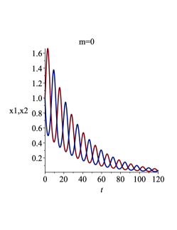
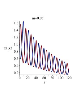
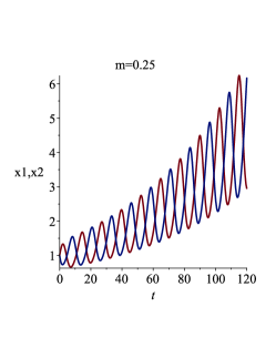
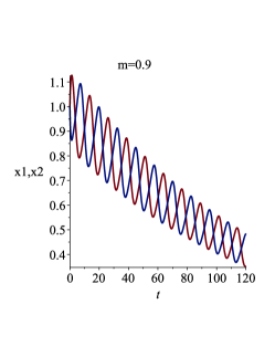
Figure 1: Solutions of (4),(5), with $r_{1}(\omega t)=-0.03+0.3\cos(\omega t),\;\;r_{2}(\omega t)=r_{1}(\omega t-\pi)$, with $\omega=0.5$, for different values of the dispersal rate $m$.

In the special case in which growth rates are constant in time ($R(\theta)\equiv R$), the growth rate $\Lambda$ is the largest eigenvalue of the matrix $R+mL$, and in this case we have $\Lambda\leq\max_{1\leq i\leq N}\bar{r}_{i}$ (see Lemma 6(iii) below), and in particular $\Lambda<0$ when all patches are sinks. Thus the DIG phenomenon cannot occur when growth rates do not vary in time.

Studying the growth or decay of the solutions of the system (3) can be formulated as a question of Floquet Theory ([Chicone 2006, Hale 2009, Klausmeier 2008]). Any system of linear differential equations with periodic coefficients has associated Floquet exponents, and indeed, in the notation used here, the value $\Lambda$ is precisely the maximal Floquet exponent - whose sign determines the growth or decay of the solutions (see Section 3.1). However, in contrast to time-independent (autonomous) systems, studying the Floquet exponents of periodic systems analytically is challenging, and our aim is to perform such a study for the particular system of interest here.

2.2 Some numerical results

A numerical demonstration of the DIG effect is shown in Figure 1, in the case $N=2$, for a pair of periodic growth-rate profiles with $\bar{r}_{1}<0,\bar{r}_{2}<0$. In the absence of dispersal ($m=0$), as well as for sufficiently weak dispersal ($m=0.05$), both populations decay, while in the presence of stronger dispersal ($m=0.25$) both populations grow - the DIG phenomenon. For yet stronger dispersal ($m=0.9$) the populations once again decay.

In Figure 2, we display a numerically-generated plot of the $(m,\omega)$ parameter-plane, for the same periodic growth profiles as in Figure 1 - the computation by which this figure was generated is explained in Section 3.2. The green region is the set of parameter values for which $\Lambda(m,\omega)>0$, that is for which DIG occurs. The lines are level curves of the function $\Lambda(m,\omega)$. As observed in the figure, there exists a value $m^{*}>0$ such that, if the dispersal rate satisfies $m\in(0,m^{*})$, DIG occurs when the frequency $\omega$ of environmental variation is sufficiently small, $0<\omega<\omega_{c}(m)$, and does not occur if $\omega>\omega_{c}(m)$, or if $m\geq m^{*}$.

Defining $\omega^{*}=\max_{m\in[0,m^{*}]}\omega_{c}(m)$, we see that if we fix a frequency $\omega\in(0,\omega^{*})$ then DIG will occur for an intermediate range of values of $m$ - neither too weak nor too strong. If $\omega>\omega^{*}$ DIG will not occur for any dispersal rate. The bottom part of Figure 2 shows the growth rate $\Lambda$ as a function of the dispersal rate $m$, for three values of the frequency, using the same profiles $r_{1}(\theta),r_{2}(\theta)$. Positive values of $\Lambda$, corresponding to DIG, occur for intermediate values of $m$.

A central aim of this work is to obtain theoretical understanding of the features noted above, as observed in Figure 2, that is to analytically derive them, thus providing a mathematical explanation for these features and proving that they are generic.

2.3 The all-sink case

We now present our main results for the case in which all patches are sinks ($\bar{r}_{i}<0$), and then discuss their implications for characterizing the conditions under which DIG occurs.

Theorem 1 (All-sink case).

Assume $r_{i}(\theta)$ ($1\leq i\leq N$) are continuous $2\pi$-periodic functions, with $\bar{r}_{i}<0$. Define

$$r_{max}(\theta)=\max_{1\leq i\leq N}r_{i}(\theta)$$

$$\chi=\frac{1}{2\pi}\int_{0}^{2\pi}r_{max}(\theta)d\theta.$$ (8)

Then we have

$$\lim_{m\rightarrow 0+}\lim_{\omega\rightarrow 0+}\Lambda(m,\omega)=\chi,$$ (9)

and

(I) If $\chi<0$ then $\Lambda(m,\omega)<0$ (decay) for all $m>0,\omega>0$.

(II) If $\chi>0$ then, defining

$$\Lambda_{0}(m)=\frac{1}{2\pi}\int_{0}^{2\pi}\lambda(R(\theta)+mL)d\theta,$$ (10)

where $\lambda(A)$ denotes the maximal eigenvalue of a symmetric matrix $A$, the equation

$$\Lambda_{0}(m)=0,\;\;m>0$$ (11)

has a unique solution $m=m^{*}>0$, and there exists a continuous function $\omega_{c}:[0,m^{*}]\rightarrow[0,\infty)$, real-analytic on $(0,m^{*})$, with $\omega_{c}(0)=\omega_{c}(m^{*})=0$ and $\omega_{c}(m)>0$ for $m\in(0,m^{*})$, such that

• If $m\in(0,m^{*})$ then $\Lambda(m,\omega)>0$ (growth) for $\omega<\omega_{c}(m)$ and $\Lambda(m,\omega)<0$ (decay) for $\omega>\omega_{c}(m)$.

• If $m\geq m^{*}$ then $\Lambda(m,\omega)<0$ (decay) for any $\omega>0$.

Example 2.

In the case $N=2$, with (4),(5), it is easy to compute (10) explicitly and find that

$$\Lambda_{0}(m)\doteq\frac{1}{2}\left[\bar{r}_{1}+\bar{r}_{2}+\frac{1}{2\pi}\int_{0}^{2\pi}\sqrt{(r_{1}(\theta)-r_{2}(\theta))^{2}+4m^{2}}d\theta\right]-m.$$ (12)

For example, taking $r_{1}(\theta),r_{2}(\theta)$ as in Figure 2, we can use (12) and solve (11) numerically, to find $m^{*}=0.7276..$ - this is the least upper bound of values of $m$ for which DIG occurs, in agreement with the top part of Figure 2.

The proof of Theorem 1 is given in Section 5, after we develop the needed tools in the sections 3, 4. We now discuss the insights that this theorem gives into the DIG effect. This can be compared with the observations regarding the numerical results made in Section 2.2 above.

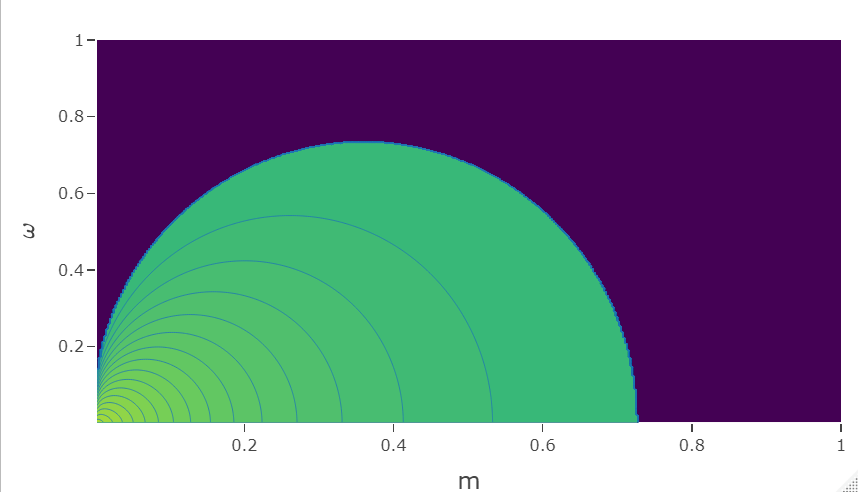
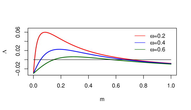
Figure 2: The two-sink case. Top: Regions of growth (green) and decay (dark) for solutions of (4),(5) in the $(m,\omega)$ parameter plane. Also shown are level curves of the function $\Lambda(m,\omega)$. Bottom: Growth rate $\Lambda$ of solutions of (4),(5) as a function of the dispersal rate $m$ for three values of the frequency $\omega$. Here $r_{1}(\omega t)=-0.03+0.3\cos(\omega t),\;\;r_{2}(\omega t)=r_{1}(\omega t-\pi)=-0.03-0.3\cos(\omega t)$.

(1) The periodic growth profiles: The condition $\chi>0$, where $\chi$ is given by (8), is necessary for DIG to occur. $\chi$ is the time-average of the maximum of the local growth rates at each point in time. This condition entails in particular that:

(i) At least one of the local growth rates must be positive at some times. However it is possible for all but one of the local growth rates to be negative at all times, and indeed it is even possible for all but one of the local growth rates to be negative and constant (time-independent) - see Figure 3 (left) for such an example.

(ii) None of the local growth rates is higher than all others at all times. Indeed if, e.g., $r_{1}(\theta)\geq r_{i}(\theta)$ for all $i$ and all $\theta$, then we have $r_{max}(\theta)=r_{1}(\theta)$, so $\chi\leq\bar{r}_{1}<0$.

(iii) The local growth rates $r_{i}(\theta)$ cannot be too similar (in particular they cannot be identical). Indeed, if $\max_{\theta}|r_{i}(\theta)-r_{j}(\theta)|\leq\epsilon$ ($1\leq i,j\leq N$) then, for all $i$,

$$\chi=\frac{1}{2\pi}\int_{0}^{2\pi}r_{max}(\theta)d\theta\leq\frac{1}{2\pi}\int_{0}^{2\pi}(r_{i}(\theta)+\epsilon)d\theta=\bar{r}_{i}+\epsilon.$$

Thus, if $\epsilon<\max_{1\leq i\leq N}|\bar{r}_{i}|$ then $\chi<0$. We therefore conclude that if

$$\max_{1\leq i,j\leq N}\max_{\theta}|r_{i}(\theta)-r_{j}(\theta)|<\max_{1\leq i\leq N}|\bar{r}_{i}|$$

then DIG cannot occur. Note, however, that it is possible to have $\chi>0$ even when all $r_{i}(\theta)$ are phase-synchronized, so that DIG can occur even if the same seasonal effect acts in all patches, as long as the strength of this effect is not identical in all patches - see Figure 3 (right) for an example.

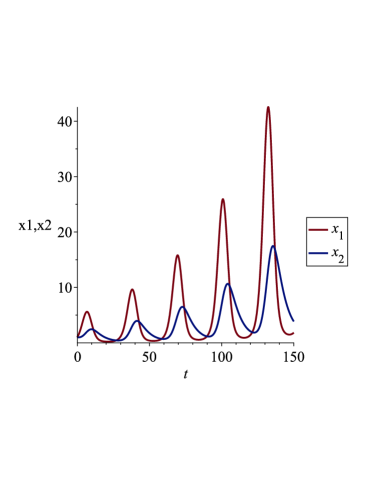
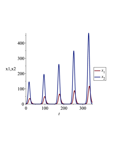
Figure 3: Left: Example of the DIG effect when growth rate in one of two patches is constant: $r_{1}(\omega t)=-0.05,\;\;r_{2}(\omega t)=-0.05+0.5\cos(\omega t)$, $\omega=0.2,m=0.1$. Right: Example of DIG when the seasonal effect in two patches is phase-synchronized: $r_{1}(\omega t)=-0.1+0.1\cos(\omega t),\;\;r_{2}(\omega t)=-0.1+0.6\cos(\omega t)$, $\omega=0.08,m=0.05$.

(2) Rate of dispersal. Assuming that $\chi>0$, part (II) of Theorem 1 implies that when $m\in(0,m^{*})$ DIG will occur for $\omega<\omega_{c}(m)$. Thus a dispersal rate which is too large ($m>m^{*}$) will prevent the DIG effect from occurring, but dispersal rates $m<m^{*}$ will induce DIG provided that the frequency $\omega$ is sufficiently small. The qualification in the previous sentence is essential: if we fix $\omega>0$, then, since $\omega_{c}(0)=0$, we will have $\omega_{c}(m)<\omega$ for $m$ sufficiently small, implying that $\Lambda(m,\omega)<0$, so that DIG does not occur.

(3) Frequency of oscillations: If $\omega>\omega^{*}=\max_{m\in[0,m^{*}]}\omega_{c}(m)$, part (II) of Theorem 1 implies that DIG will not occur. Thus, while time-variation of at least one growth rate is essential for DIG, the frequency of this variation cannot be too high.

2.4 The Source-Sink case

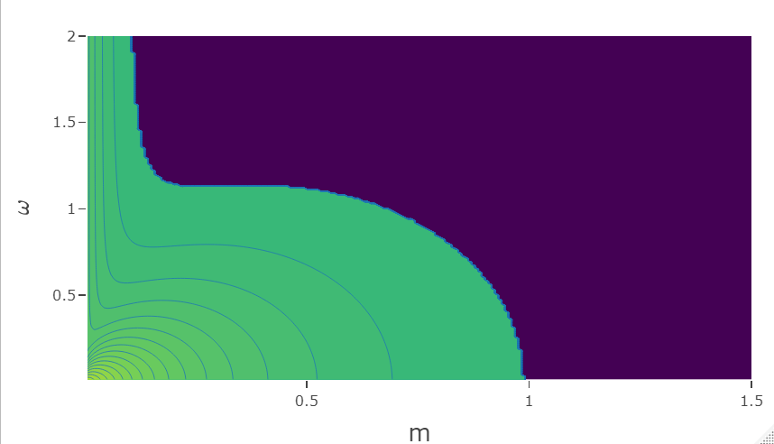
Figure 4: The Source-Sink case: Regions of growth (green) and decay (dark) for solutions of (4),(5) in the $(m,\omega)$ parameter plane. Also shown are level curves of the function $\Lambda(m,\omega)$. Here $r_{1}(\omega t)=-0.1+0.3\cos(\omega t),\;\;r_{2}(\omega t)=0.05-0.3\cos(\omega t)$.

Although our main interest is in the DIG effect, which involves the all-sink case, we complement our analysis with a treatment of the source-sink case, using the same methods. Our results in this case are given by

Theorem 2 (Source-Sink case).

Assume $r_{i}(\theta)$ ($1\leq i\leq N$) are continuous $2\pi$-periodic functions, with

$$\min_{1\leq i\leq N}\bar{r}_{i}<0,\;\;\;\max_{1\leq i\leq N}\bar{r}_{i}>0.$$ (13)

Denote

$$\bar{R}=\left(\begin{array}[]{ccc}\bar{r}_{1}&0&0\\ 0&\ddots&0\\ 0&0&\bar{r}_{N}\end{array}\right),\;\;\;\;\;\bar{r}=\frac{1}{N}\sum_{i=1}^{n}\bar{r}_{i}.$$ (14)

(I) If $\bar{r}>0$ then for any $m>0,\omega>0$ we have $\Lambda(m,\omega)>0$ (growth).

(II) If $\bar{r}<0$ then the equation (11) has a unique solution $m=m^{*}>0$.

Defining

$$\Lambda_{\infty}(m)=\lambda\left(\bar{R}+mL\right),$$ (15)

where $\lambda(A)$ denotes the maximal eigenvalue of a symmetric matrix $A$, the equation

$$\Lambda_{\infty}(m)=0,\;\;\;m>0$$ (16)

has a unique solution, which we denote by $\hat{m}$, and we have $\hat{m}\leq m^{*}$. Unless $r_{i}(\theta)-r_{j}(\theta)$ are constant for all $i,j$, we have strict inequality $\hat{m}<m^{*}$, and there exists a continuous function $\omega_{c}:(\hat{m},m^{*}]\rightarrow[0,\infty)$, real-analytic on $(\hat{m},m^{*})$, with $\lim_{m\rightarrow\hat{m}+}\omega_{c}(m)=+\infty$, $\omega_{c}(m^{*})=0$, and $\omega(m)>0$ for $m\in(\hat{m},m^{*})$, such that

• If $m\in(0,\hat{m}]$ then for any $\omega>0$ we have $\Lambda(m,\omega)>0$ (growth).

• If $m\in(\hat{m},m^{*})$ then for $\omega\in(0,\omega_{c}(m))$ we have $\Lambda(m,\omega)>0$ (growth) and for $\omega>\omega_{c}(m)$ we have $\Lambda(m,\omega)<0$ (decay).

• If $m\geq m^{*}$ then for all $\omega>0$ we have $\Lambda(m,\omega)<0$ (decay).

The proof of Theorem 2 is given in Section 5.

Part (I) of the above theorem says that when the mean of the time-averaged local growth rates is positive, growth always occurs. Part (II) says that growth may occur also when the mean of the time-averaged growth rates is negative, and - in contrast with the all-sink case - here, if $m$ is sufficiently small ($m<\hat{m}$), we have $\Lambda(m,\omega)>0$ (growth) for all $\omega>0$. This can be seen in the parameter-plane diagram in Figure 4, obtained numerically. Let us note that the condition $m<\hat{m}$ is precisely the condition for growth in the case in which the local growth rates $r_{i}(\theta)$ are constant, with values $\bar{r}_{i}$ (with $\min_{1\leq i\leq N}\bar{r}_{i}<0$, $\max_{1\leq i\leq N}\bar{r}_{i}>0$), that is the condition under which the largest eigenvalue of the matrix $\bar{R}+mL$ is positive. However, unless all $r_{i}(\theta)-r_{j}(\theta)$ are constant, we have $\hat{m}<m^{*}$, and the theorem implies that, when the frequency is sufficiently small, the time periodic system also displays growth for parameter values $m\in(\hat{m},m^{*})$ for which the corresponding time-averaged system leads to decay.

We note that the special case in which all $r_{i}(\theta)-r_{j}(\theta)$ are constant, which was excluded in the above theorem, is a trivial one: in this case we have $R(\theta)=\bar{R}+r_{0}(\theta)I$, where $r_{0}(\theta)$ is $2\pi$-periodic and satisfies $\int_{0}^{2\pi}r_{0}(\theta)d\theta=0$, and then (3) has the explicit solution $\mathbb{x}(t)=e^{\int_{0}^{t}r_{0}(\omega s)ds}e^{t(\bar{R}+mL)}\mathbb{x}(0)$, from which it follows that $\Lambda(m,\omega)=\lambda(\bar{R}+mL)=\Lambda_{\infty}(m)$ for all $\omega$, so that the growth rate is identical to that of the corresponding time-averaged system for all $(m,\omega)$.

Example 3.

In the case $N=2$, with (4),(5), and assuming the source-sink case $\bar{r}_{1}\bar{r}_{2}<0$, it is easy to compute (15) explicitly and find that

$$\Lambda_{\infty}(m)=\frac{1}{2}\left[\bar{r}_{1}+\bar{r}_{2}+\sqrt{(\bar{r}_{1}-\bar{r}_{2})^{2}+4m^{2}}\right]-m.$$

The solution $\hat{m}$ of (16) is then given by

$$\hat{m}=\left(\frac{1}{\bar{r}_{1}}+\frac{1}{\bar{r}_{2}}\right)^{-1}.$$ (17)

For example, taking $r_{1}(\theta),r_{2}(\theta)$ as in Figure 4, (17) gives $\hat{m}=0.1$, so that by Theorem 2, for $m\leq{\hat{m}}$ we have $\Lambda(m,\omega)>0$ for all $\omega$. Using (12) and solving (11) numerically, we find $m^{*}=0.990..$. Thus for $\hat{m}<m<m^{*}$ we have $\Lambda(m,\omega)>0$ for $\omega$ small, and $\Lambda(m,\omega)<0$ for $\omega$ large, and for $m>m^{*}$ we always have $\Lambda(m,\omega)<0$. All these results are in agreement with Figure 4.

3 Characterizations of the growth rate

In this section we characterize the growth rate $\Lambda(m,\omega)$ corresponding to (3) in different ways, each of which has its uses: as the dominant eigenvalue of a monodromy matrix, as the principal eigenvalue of a periodic problem, and, in the case of two patches, via an integral related to a periodic solution of an associated nonlinear scalar differential equation.

3.1 The growth rate as a principal eigenvalue

The fundamental solution corresponding to (3) is the matrix function $X(t)$ satisfying

$$X^{\prime}(t)=[R(\omega t)+mL]X(t),\;\;\;X(0)=I,$$

where $I$ is the identity matrix. Since the matrix $R(\omega t)+mL$ is an irreducible cooperative matrix (i.e. has non-negative non-diagonal entries), the Kamke-Müller theorem [Hirsch and Smith 2006] implies that the matrices $X(t)$ have positive entries - so that solutions of (3) with positive initial conditions remain positive for all time. The Perron-Frobenius theorem implies that the matrix $X(T)$ ($T=\frac{2\pi}{\omega}$), known as the monodromy matrix, has a dominant eigenvalue (an eigenvalue of maximal modulus) $\rho=\rho(X(T))$ which is positive and simple, and the corresponding eigenvector $\mathbb{v}$ has positive entries and is the only positive eigenvector of $X(T)$. By Floquet’s Theorem (see, e.g., [Chicone 2006], Theorem 2.83) we have $X(t+T)=X(t)X(T)$ for all $t$. Therefore, defining

$$\lambda=\frac{1}{T}\ln\left(\rho(X(T))\right),\;\;\varphi(t)=e^{-\lambda t}X(t)\mathbb{v},$$ (18)

($\lambda$ is known as the Floquet exponent), we have that

$$\varphi\left(t+T\right)=e^{-\lambda\left(t+T\right)}X\left(t+T\right)\mathbb{v}=\frac{1}{\rho}e^{-\lambda t}X(t)X(T)\mathbb{v}=e^{-\lambda t}X(t)\mathbb{v}=\varphi(t),$$

$$\varphi^{\prime}(t)=-\lambda e^{-\lambda t}X(t)\mathbb{v}+e^{-\lambda t}X^{\prime}(t)\mathbb{v}=[R(\omega t)+mL]\varphi(t)-\lambda\varphi(t).$$

Thus $\lambda$ given by (18) is the principal eigenvalue (the one with largest real part) of the periodic problem

$$\varphi^{\prime}(t)=[R(\omega t)+mL]\varphi(t)-\lambda\varphi(t),\;\;\;\;\varphi\left(t+T\right)=\varphi(t).$$

Moreover, we have that, for any positive solution $\mathbb{x}(t)$ of (3):

$$\underline{C}\leq\frac{x_{i}(t)}{e^{\lambda t}\varphi_{i}(t)}\leq\overline{C},\;\;\;\;\;1\leq i\leq N,$$ (19)

where the positive constants $\underline{C},\overline{C}$ depend on the initial conditions - for an elegant proof of this fact using the relative entropy method see [Perthame 2007], Sec. 6.3.2. (19), together with the periodicity of $\varphi(t)$ imply

$$\Lambda[x_{i}]=\lim_{t\rightarrow\infty}\frac{1}{t}\ln(x_{i}(t))=\lambda.$$ (20)

In particular this shows that, under coupling, the growth rates in all patches are identical. We note also that by the analytic dependence of solutions of differential equations on parameters, and the fact that $\rho(X(T))$ is a simple eigenvalue, (20) implies that the function $\Lambda(m,\omega)$ is real-analytic.

We can also normalize the period, setting $\varphi(t)=\mathbb{u}(\omega t)$, where $\mathbb{u}(\theta)$ is $2\pi$-periodic, and we thus obtain

Lemma 1.

The growth rate $\Lambda(m,\omega)$ is given as

$$\Lambda(m,\omega)=\lambda,$$

where $\lambda$ is the principal eigenvalue of the periodic problem

$$\omega\mathbb{u}^{\prime}(\theta)=[R(\theta)+mL]\mathbb{u}(\theta)-\lambda\mathbb{u}(\theta),$$

$$\mathbb{u}(\theta+2\pi)=\mathbb{u}(\theta),$$ (21)

that is the eigenvalue with largest real part.

We now cite an important result from [Liu et al. 2022] which will play a significant role in the proofs of the main results.

Lemma 2.

For all $m>0,\omega>0$ we have $\Lambda_{\omega}^{\prime}(m,\omega)\leq 0$. The inequality is strict except in the case that $r_{i}(\theta)-r_{j}(\theta)$ are constants for all $i,j$, so that $\Lambda(m,\omega)$ is strictly decreasing in $\omega$ for any fixed $m$.

In view of Lemma 1, this result follows from Part (ii) of Theorem 1.1 in [Liu et al. 2022] and Remark 1.2 following that theorem. Note that in the formulation of the results in [Liu et al. 2022] the principal eigenvalue is defined as the negative of the value as defined here, and is thus increasing with respect to $\omega$.

3.2 An associated scalar differential equation in the two-patch case

In the case of two patches ($N=2$) we now obtain a formula for the growth rate $\Lambda$ in terms of the periodic solution of an associated nonlinear scalar differential equation. This formula, besides its intrinsic interest, has been useful for us in carrying out numerical computations.

Lemma 3.

If $(x_{1}(t),x_{2}(t))$ is any positive solution of (4),(5), then the function

$$z(t)=\frac{x_{2}(t)}{x_{1}(t)}.$$ (22)

satisfies the differential equation

$$z^{\prime}=(r_{2}(\omega t)-r_{1}(\omega t))z+m(1-z^{2}).$$ (23)

Proof.

Dividing (4),(5) by $x_{1}$ we have

$$\frac{x_{1}^{\prime}(t)}{x_{1}(t)} = r_{1}(\omega t)+mz(t)-m,$$ (24)

$$\frac{x_{2}^{\prime}(t)}{x_{1}(t)} = r_{2}(\omega t)z(t)+m-mz(t),$$

from which it follows that

$$z^{\prime}(t) = \frac{x_{1}(t)x_{2}^{\prime}(t)-x_{1}^{\prime}(t)x_{2}(t)}{x_{1}(t)^{2}}=\frac{x_{2}^{\prime}(t)}{x_{1}(t)}-\frac{x_{1}^{\prime}(t)}{x_{1}(t)}\cdot z(t)$$

$$= r_{2}(\omega t)z(t)+m-mz(t)-(r_{1}(\omega t)+mz(t)-m)\cdot z(t)$$

$$= (r_{2}(\omega t)-r_{1}(\omega t))z(t)+m(1-z(t)^{2}).$$

∎

Regarding the differential equation (23), we note that $z=0$ implies $z^{\prime}>0$, so that any solution with positive initial condition remains positive for all $t>0$. Moreover the following lemma shows that all solutions of (23) approach a unique periodic solution as $t\rightarrow\infty$, and that this periodic solution can be used to compute the growth rate $\Lambda(m,\omega)$.

Lemma 4.

Assume $m>0$. For each $\omega>0$, there exists a unique $\frac{2\pi}{\omega}$-periodic solution of (23), which we denote by $z_{p}(t)$, and this solution is globally stable, that is, all solutions $z(t)$ of (23) with $z(0)>0$ satisfy

$$\lim_{t\rightarrow\infty}[z(t)-z_{p}(t)]=0.$$ (25)

The growth rate of solutions of (4),(5) is given by

$$\Lambda(m,\omega)=\frac{1}{2}\left(\bar{r}_{1}+\bar{r}_{2}\right)+m\cdot\left(\frac{\omega}{4\pi}\int_{0}^{\frac{2\pi}{\omega}}\left(z_{p}(\tau)+\frac{1}{z_{p}(\tau)}\right)d\tau-1\right).$$ (26)

Proof.

We first transform (23) by making the change of variable $z(t)=e^{y(t)}$ (using the fact that $z(t)$ is positive), to obtain the equation

$$y^{\prime}=(r_{2}(\omega t)-r_{1}(\omega t))+m(e^{-y}-e^{y}).$$ (27)

We will show that (27) has a unique $\frac{2\pi}{\omega}$-periodic solution $y_{p}(t)$ which is globally stable in the sense that, for any solution $y(t)$ of (27),

$$\lim_{t\rightarrow\infty}[y(t)-y_{p}(t)]=0.$$

This will imply the result of Lemma 4 for the equation (23), with $z_{p}(t)=e^{y_{p}(t)}$. Denote by $y(t,y_{0})$ the solution of (27) satisfying the initial condition $y(0)=y_{0}$. We define $\psi$ to be the time-$T$ ($T=\frac{2\pi}{\omega}$) Poincaré mapping corresponding to (27):

$$\psi(y_{0})=y\left(T,y_{0}\right).$$

To compute the derivative of this function we differentiate the equations

$$y_{t}(t,y_{0})=(r_{2}(\omega t)-r_{1}(\omega t))+m[e^{-y(t,y_{0})}-e^{y(t,y_{0})}],\;\;\;y(0,y_{0})=y_{0}$$

with respect to $y_{0}$, obtaining

$$y_{y_{0}t}(t,y_{0})=-m[e^{-y(t,y_{0})}+e^{y(t,y_{0})}]y_{y_{0}}(t,y_{0})\;\;\;y_{y_{0}}(0,y_{0})=1,$$

leading to

$$y_{y_{0}}(t,y_{0})=e^{-m\int_{0}^{t}(e^{-y(\tau,y_{0})}+e^{y(\tau,y_{0})})d\tau},$$

so that

$$\psi^{\prime}(y_{0})=y_{y_{0}}(T,y_{0})=e^{-m\int_{0}^{T}(e^{-y(\tau,y_{0})}+e^{y(\tau,y_{0})})d\tau}$$

satisfies $0<\psi^{\prime}(y_{0})<e^{-2mT}<1$ for all $y_{0}$. This implies that $\psi:\mathbb{R}\rightarrow\mathbb{R}$ is a contraction mapping, so that by Banach’s contraction mapping principle ([Hale 2009], Section 0.3) it has a unique fixed point $y^{*}\in\mathbb{R}$, and, for all $y_{0}\in\mathbb{R}$, the iterates of $\psi$ satisfy $\lim_{k\rightarrow\infty}\psi^{k}(y_{0})=y^{*}$. This, in turn, implies that the function $y_{p}(t)=y(t,y^{*})$ is a $T$-periodic solution of (27), which is globally stable.

We now show that the periodic solution $z_{p}$ determines the growth rate $\Lambda$ of $x_{1},x_{2}$. By (24) and (25) we have

$$\lim_{t\rightarrow\infty}\frac{1}{t}\ln\left(x_{1}(t)\right)=\lim_{t\rightarrow\infty}\frac{1}{t}\int_{0}^{t}\frac{x_{1}^{\prime}(\tau)}{x_{1}(\tau)}d\tau$$

$$=\lim_{t\rightarrow\infty}\frac{1}{t}\left[\int_{0}^{t}r_{1}(\omega\tau)d\tau+m\int_{0}^{t}(z(\tau)-1)d\tau\right]=\bar{r}_{1}+m\cdot\left(\frac{\omega}{2\pi}\int_{0}^{\frac{2\pi}{\omega}}z_{p}(\tau)d\tau-1\right).$$

Note also that, by (22), and since (25) implies that any solution $z(t)$ of (23) is bounded on $[0,\infty)$, we have

$$\lim_{t\rightarrow\infty}\frac{1}{t}\ln(x_{2}(t))=\lim_{t\rightarrow\infty}\frac{1}{t}\left[\ln(z(t))+\ln(x_{1}(t))\right]=\lim_{t\rightarrow\infty}\frac{1}{t}\ln(x_{1}(t)).$$

We thus have

$$\Lambda[x_{1}]=\Lambda[x_{2}]=\Lambda(m,\omega)=\bar{r}_{1}+m\cdot\left(\frac{\omega}{2\pi}\int_{0}^{\frac{2\pi}{\omega}}z_{p}(\tau)d\tau-1\right).$$ (28)

By exchanging the roles of $r_{1}(\theta)$ and $r_{2}(\theta)$, so that $z_{p}$ is replaced by $\frac{1}{z_{p}}$ we get the equivalent expression

$$\Lambda(m,\omega)=\bar{r}_{2}+m\cdot\left(\frac{\omega}{2\pi}\int_{0}^{\frac{2\pi}{\omega}}\frac{1}{z_{p}(\tau)}d\tau-1\right),$$ (29)

and by averaging (28),(29) we obtain the symmetric expression (26). ∎

We note that the plots in Figures 2,4 were obtained by using Lemma 4: For each point in a grid in the plotted region, the periodic solution $z_{p}$ was found numerically, and the quantity $\Lambda(m,\omega)$ was computed using (28). The green (growth) region is the set of points for which $\Lambda(m,\omega)>0$.

4 The low and high frequency limits of the growth rate

The characterization of the growth rate $\Lambda$ in terms of the principal eigenvalue of a periodic problem (Lemma 1) allows us to employ the recent results of [Liu et al. 2022], which determine the limit of $\Lambda(m,\omega)$ in the cases $\omega\rightarrow 0$ and $\omega\rightarrow\infty$, and thus provide a key element in the proofs of Theorems 1,2. In this section, we cite results from [Liu et al. 2022] and apply them to our specific problem.

4.1 The low frequency limit

We now present an explicit expression for the growth rate $\Lambda(m,\omega)$ in the limit $\omega\rightarrow 0$ (see Figure 5 for a numerical illustration of the contents of this result).

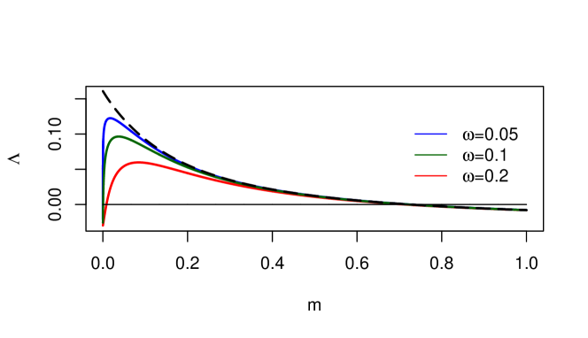
Figure 5: Illustration of the result of Lemma 5. Here $r_{1}(\omega t)=-0.03+0.3\cos(\omega t),\;\;r_{2}(\omega t)=r_{1}(\omega t-\pi)$. The curves $m\rightarrow\Lambda(m,\omega)$ are plotted for $\omega=0.2,0.1,0.05$, and they can be seen to converge to the curve $\Lambda_{0}(m)$ (dashed line).

Theorem 2.1 of [Liu et al. 2022] (in the case $a=0$ of that theorem), applied to the periodic eigenvalue problem (1), gives:

Lemma 5.

Let $\Lambda_{0}(m)$ be defined by (10). Then we have, for each $m>0$:

$$\lim_{\omega\rightarrow 0+}\Lambda(m,\omega)=\Lambda_{0}(m).$$

The auxilliary results in the following lemma will be needed below.

Lemma 6.

Let $L$ be an $N\times N$ symmetric matrix with non-negative non-diagonal elements, which is irreducible, and satisfies (2). Let

$$D=\left(\begin{array}[]{ccc}d_{1}&0&0\\ 0&\ddots&0\\ 0&0&d_{N}\end{array}\right)$$

be a diagonal matrix. Then

(i) If the numbers $d_{i}$ ($1\leq i\leq N$) are not all equal to each other, then $\lambda(D+mL)$ is strictly monotone decreasing with respect to $m$. If $d_{i}=d$, for all $i$ then $\lambda(D+mL)=d$.

(ii) As $m\rightarrow\infty$, we have

$$\lim_{m\rightarrow\infty}\lambda(D+mL)=\frac{1}{N}\sum_{i=1}^{N}d_{i}.$$

(iii) $\lambda(D+mL)<\max_{1\leq i\leq N}d_{i}$ for all $m$.

Proof.

Since $L$ has non-negative non-diagonal elements, is irreducible, and satisfies (2), the Perron-Frobenius theorem implies that its maximal eigenvalue is $\lambda(L)=0$, with corresponding eigenvector $\mathbb{1}=(1,1,\cdots,1)$. Note that $\lambda(L)=0$ means that $L$ is negative semi-definite.

If $A,B$ are symmetric matrices and $B$ is positive semi-definite, then $\lambda(A+B)\geq\lambda(A)$ - this is a consequence of the min-max principle (see e.g., [Bhatia 1997], Corrollary III.2.3). Apply this with $A=D+m_{2}L$, $B=(m_{1}-m_{2})L$, where $0\leq m_{1}<m_{2}$ - note that $B$ is positive semi-definite since $L$ is negative semi-definite - to conclude that $\lambda(D+m_{2}L)=\lambda(A)\leq\lambda(A+B)=\lambda(D+m_{1}L)$. We have therefore shown that $\lambda(D+mL)$ is monotone decreasing (the fact that it is strictly decreasing when the $d_{i}$’s are not all equal will be shown below).

To prove (ii), note that $\lambda(D+mL)=m\cdot\lambda(L+m^{-1}D)$, and study the maximal eigenvalue of $L+\epsilon D$ for small $\epsilon$. As $\epsilon\rightarrow 0+$, each of eigenvalues of $M(\epsilon)=L+\epsilon D$ converges to a corresponding eigenvalue of $L$ (see e.g. [Bhatia 1997], Corollary III.2.6), and since the maximal eigenvalue of $L$ is $0$, the maximal eigenvalue of $M(\epsilon)$, which we denote by $\mu(\epsilon)$, satisfies $\lim_{\epsilon\rightarrow 0}\mu(\epsilon)=0$. Denoting the eigenvector corresponding to $\mu(\epsilon)$ by $\mathbb{v}(\epsilon)$, we have $\mathbb{v}(0)=\mathbb{1}=(1,1,\cdots,1)$ and

$$M(\epsilon)\mathbb{v}(\epsilon)=\mu(\epsilon)\mathbb{v}(\epsilon)\;\;\Rightarrow\;\;M^{\prime}(\epsilon)\mathbb{v}(\epsilon)+M(\epsilon)\mathbb{v}^{\prime}(\epsilon)=\mu^{\prime}(\epsilon)\mathbb{v}(\epsilon)+\mu(\epsilon)\mathbb{v}^{\prime}(\epsilon).$$

Setting $\epsilon=0$ and denoting by $\langle\cdot,\cdot\rangle$ the standard inner product on $\mathbb{R}^{N}$, we get

$$D\mathbb{1}+L\mathbb{v}^{\prime}(0)=\mu^{\prime}(0)\mathbb{1}\;\;\Rightarrow\;\;\langle D\mathbb{1},\mathbb{1}\rangle+\langle L\mathbb{v}^{\prime}(0),\mathbb{1}\rangle=\mu^{\prime}(0)\langle\mathbb{1},\mathbb{1}\rangle,$$

and since by symmetry of $L$ we have $\langle L\mathbb{v}^{\prime}(0),\mathbb{1}\rangle=\langle\mathbb{v}^{\prime}(0),L\mathbb{1}\rangle=0$, we conclude that

$$\mu^{\prime}(0)=\frac{\langle D\mathbb{1},\mathbb{1}\rangle}{\langle\mathbb{1},\mathbb{1}\rangle}=\frac{1}{N}\sum_{i=1}^{N}d_{i},\;\;\;\Rightarrow\;\;\;\mu(\epsilon)=\mu^{\prime}(0)\epsilon+O(\epsilon^{2})=\frac{\epsilon}{N}\sum_{i=1}^{N}d_{i}+O(\epsilon^{2}).$$

Therefore, as $m\rightarrow\infty$,

$$\lambda(D+mL) = m\cdot\lambda(L+m^{-1}D)=m\cdot\left(\frac{m^{-1}}{N}\sum_{i=1}^{N}d_{i}+O(m^{-2})\right)$$

$$= \frac{1}{N}\sum_{i=1}^{N}d_{i}+O(m^{-1}),$$

proving (ii).

We now note that, since the function $m\rightarrow\lambda(D+mL)$ is real-analytic, it cannot be constant on an interval unless it is everywhere constant, but if this is the case then part (ii) implies that

$$\frac{1}{N}\sum_{i=1}^{N}d_{i}=\lim_{m\rightarrow\infty}\lambda(D+mL)=\lambda(D)=\max_{1\leq i\leq N}d_{i},$$

which occurs iff all $d_{i}$’s are equal. Therefore if the $d_{i}$’s are not equal we have that $m\rightarrow\lambda(D+mL)$ is strictly decreasing, and when the all $d_{i}$’s are equal, it is constant.

(iii) follows from (i), since $\lambda(D+mL)\leq\lambda(D)=\max_{1\leq i\leq N}d_{i}$. ∎

In the following lemma we derive properties of the function $\Lambda_{0}(m)$, which will be used in the proofs of the main theorems:

Lemma 7.

(i) $\Lambda_{0}(0)=\chi$, where $\chi$ is given by (8).

(ii) $\lim_{m\rightarrow\infty}\Lambda_{0}(m)=\bar{r}\doteq\frac{1}{N}\sum_{i=1}^{N}\bar{r}_{i}$.

(iii) Assuming that it is not the case that $r_{i}(\theta)\equiv r_{j}(\theta)$ for all $i,j$, the function $\Lambda_{0}(m)$ is strictly monotone decreasing on $[0,\infty)$.

(iv) If $\chi<0$ then $\Lambda_{0}(m)<0$ for all $m>0$.

(v) If $\chi>0$ and $\bar{r}<0$, there is a unique value $m^{*}$ such that $\Lambda_{0}(m^{*})=0$, that is a solution of the equation (11), and we have

$$m\in(0,m^{*})\;\; \Rightarrow \;\;\Lambda_{0}(m)>0,$$

$$m>m^{*}\;\; \Rightarrow \;\;\Lambda_{0}(m)<0.$$ (30)

Proof.

(i) Since $R(\theta)$ is a diagonal matrix we have $\lambda(R(\theta))=r_{max}(\theta)$, hence by the definition (10) of $\Lambda_{0}(m)$, we have

$$\Lambda_{0}(0)=\frac{1}{2\pi}\int_{0}^{2\pi}\lambda(R(\theta))d\theta=\frac{1}{2\pi}\int_{0}^{2\pi}r_{max}(\theta)d\theta=\chi.$$

(ii) Fixing $\theta$ and applying Lemma 6(ii) with $D=R(\theta)$ we have

$$\lim_{m\rightarrow\infty}\lambda(R(\theta)+mL)=\frac{1}{N}\sum_{i=1}^{N}r_{i}(\theta).$$ (31)

Since, by Lemma 6(i), $\lambda(R(\theta)+mL)$ is monotone decreasing or constant with respect to $m$ for each fixed $\theta$, Lebesgue’s Monotone Convergence Theorem ([Rudin 1976], Th. 11.28) and (31) imply

$$\lim_{m\rightarrow\infty}\Lambda_{0}(m)=\frac{1}{2\pi}\lim_{m\rightarrow\infty}\int_{0}^{2\pi}\lambda(R(\theta)+mL)d\theta=\frac{1}{2\pi}\frac{1}{N}\int_{0}^{2\pi}\sum_{i=1}^{N}r_{i}(\theta)d\theta=\bar{r}.$$

(iii) By Lemma 6(i) $\lambda(R(\theta)+mL)$ is monotone decreasing or constant with respect to $m$ for any value of theta $\theta$, and it is strictly monotone decreasing unless all $r_{i}(\theta)$’s are equal, so the definition (10) implies that $\Lambda_{0}(m)$ is strictly monotone increasing unless all $r_{i}(\theta)$’s are everywhere equal.

(iv) follows from (i) and (iii).

(v) If $\chi>0$ and $\bar{r}<0$ then by (i),(ii) we have $\Lambda_{0}(0)>0$, $\lim_{m\rightarrow\infty}\Lambda_{0}(m)<0$, and since by (iii) the function $\Lambda_{0}(m)$ is strictly decreasing (note that $\chi>0$, $\bar{r}<0$ preclude the possibility that all $r_{i}(\theta)$ are indentical) we conclude that there exists a unique $m^{*}>0$ with $\Lambda_{0}(m)=0$, and that (7) holds. ∎

4.2 The high frequency limit

We now study the behavior of $\Lambda(m,\omega)$ in the limit $\omega\rightarrow\infty$.

Theorem 1.2 of [Liu et al. 2022] tells us that

Lemma 8.

Let $\Lambda_{\infty}(m)$ be defined by (15). Then we have, for all $m>0$,

$$\lim_{\omega\rightarrow\infty}\Lambda(m,\omega)=\Lambda_{\infty}(m).$$

We now derive properties of the function $\Lambda_{\infty}(m)$, which will be used in the proofs of the main theorems.

Lemma 9.

(i) $\Lambda_{\infty}(0)=\max_{1\leq i\leq N}\bar{r}_{i}$.

(ii) $\lim_{m\rightarrow\infty}\Lambda_{\infty}(m)=\bar{r}\doteq\frac{1}{N}\sum_{i=1}^{N}\bar{r}_{i}.$

(iii) $\Lambda_{\infty}(m)$ is strictly monotone decreasing, except in the case that $\bar{r}_{i}=\bar{r}_{j}$ for all $i,j$, in which it is constant.

(iv) For all $m>0$ we have $\Lambda_{\infty}(m)\leq\Lambda_{0}(m)$, with strict inequality unless all functions $r_{i}(\theta)-r_{j}(\theta)$ are constant.

(v) When $\bar{r}>0$ we have $\Lambda_{\infty}(m)>0$ for all $m>0$.

(vi) When $\bar{r}_{i}<0$ for all $i$, we have $\Lambda_{\infty}(m)<0$ for all $m>0$.

(vii) When $\bar{r}<0$ and (13) holds, the equation (16) has a unique solution $\hat{m}$, and

$$m\in(0,\hat{m})\;\;\Rightarrow\;\;\Lambda_{\infty}(m)>0,$$

$$m>\hat{m}\;\;\Rightarrow\;\;\Lambda_{\infty}(m)<0.$$ (32)

Proof.

(i) $\Lambda_{\infty}(0)=\lambda(\bar{R})=\max_{1\leq i\leq N}\bar{r}_{i}$.

(ii) and (iii) follow from Lemma 6(i),(ii) taking $D=\bar{R}$.

(iv) follows by combining the results of Lemmas 2, 5 and 8: since $\Lambda(m,\omega)$ is monotone decreasing in $\omega$,

$$\Lambda_{\infty}(m)=\lim_{\omega\rightarrow\infty}\Lambda(m,\omega)\leq\lim_{\omega\rightarrow 0+}\Lambda(m,\omega)=\Lambda_{0}(m).$$

Unless all $r_{i}(\theta)-r_{j}(\theta)$ are constant, Lemma 2 implies that the inequality is strict.

(v) Follows from (ii) and (iii).

(vi) Follows from (i) and (iii).

(vii) If $\bar{r}<0$ and (13) holds, then by (i) we have $\Lambda_{\infty}(0)>0$, by (ii) we have $\lim_{m\rightarrow\infty}\Lambda_{\infty}(m)<0$, and by (iii) we have that $\Lambda_{\infty}(m)$ is strictly monotone decreasing. Hence there is a unique value $\hat{m}\in(0,\infty)$ such that $\Lambda_{\infty}(\hat{m})=0$, and (9) holds. ∎

5 Proofs of the main theorems

We now combine the results obtained in the previous sections to obtain the proofs of the main theorems.

Proof of Theorem 1.

Here we assume the all-sink case, $\bar{r}_{i}<0$ for $1\leq i\leq N$.

Let $\chi$ be defined by (8). (9) follows from Lemma 5 and Lemma 7(i).

If $\chi<0$ then Lemma 7(iv) and Lemma 5 imply that, for any $m>0$, we have $\Lambda(m,\omega)<0$ for $\omega$ sufficiently small, hence Lemma 2 implies that $\Lambda(m,\omega)<0$ for all $\omega$. Therefore we have part (I) of Theorem 1.

We now assume $\chi>0$. Lemma 7(v) then implies that there is a unique solution $m^{*}$ of the equation (11), and that (7) holds. Also, by Lemma 9(vi), we have that

$$\Lambda_{\infty}(m)<0,\;\;\;m\in(0,\infty).$$ (33)

By Lemma 2, we have that $\Lambda(m,\omega)$ is strictly monotone decreasing with respect to $\omega$ - indeed it is impossible that $r_{i}(\theta)-r_{j}(\theta)$ are constant for all $i,j$, since this would imply that one the functions $r_{i}(\theta)$ is larger than all the others, leading to $\chi=\bar{r}_{i}<0$, in contradiction with our assumption $\chi>0$.

We first prove part (II)b, fixing $m>m^{*}$. (7) and Lemma 5 imply that $\Lambda(m,\omega)<0$ for $\omega$ sufficiently small, and since $\Lambda(m,\omega)$ is monotone decreasing with respect to $\omega$, we have $\Lambda(m,\omega)<0$ for all $\omega>0$. Note also that by continuity this implies $\Lambda(m^{*},\omega)\leq 0$ for all $\omega$, and since $\Lambda(m^{*},\omega)$ is strictly decreasing with respect to $\omega$ we conclude that $\Lambda(m^{*},\omega)<0$ also holds. We thus have (II)(b).

To prove part (II)(a) of the theorem, we now fix $m\in(0,m^{*})$. (7) and Lemma 5 imply that $\Lambda(m,\omega)>0$ for $\omega>0$ sufficiently small, while (33) and Lemma 8 imply that $\Lambda(m,\omega)<0$ for $\omega>0$ sufficiently large. By the monotonicity of $\Lambda(m,\omega)$ with respect to $\omega$, the above two facts imply that there exists a unique value $\omega=\omega_{c}(m)>0$ for which $\Lambda(m,\omega)=0$, and we have

$$\omega\in(0,\omega_{c}(m))\;\; \Rightarrow \;\;\Lambda(m,\omega)>0$$

$$\omega>\omega_{c}(m)\;\; \Rightarrow \;\;\Lambda(m,\omega)<0.$$ (34)

Since the function $\Lambda(m,\omega)$ is real-analytic (see remark preceding Lemma 1), and $\omega_{c}(m)$ is defined implicitly by $\Lambda(m,\omega_{c}(m))=0$ (for $m\in(0,m^{*})$), and $\Lambda_{\omega}^{\prime}(m,\omega_{c}(m))<0$ (Lemma 2), the real-analytic implicit function theorem (see, e.g., [Krantz and Parks 2002], Section 6.1) implies that $\omega_{c}(m)$ is a real-analytic function.

To complete the proof we show that the function $\omega_{c}(m)$ can be continuously extended to the closed interval $[0,m^{*}]$, with $\omega_{c}(0)=\omega_{c}(m^{*})=0$. To show that $\lim_{m\rightarrow 0+}\omega_{c}(m)=0$, we fix $\omega_{0}>0$ and show that $\omega_{c}(m)<\omega_{0}$ for $m$ sufficiently small. Indeed, since $\bar{r}_{i}<0$ for all $i$, we know by (7) that for $m=0$ we have $\Lambda(0,\omega_{0})=\max_{1\leq i\leq N}\bar{r}_{i}<0$, hence by continuity $\Lambda(m,\omega_{0})<0$ for $m$ sufficiently small, so that, for such $m$, (5) implies $\omega_{c}(m)<\omega_{0}$. Similarly, to show that $\lim_{m\rightarrow m^{*}-}\omega_{c}(m)=0$, we fix $\omega_{0}>0$ and show that $\omega_{c}(m)<\omega_{0}$ for $m<m^{*}$ sufficiently close to $m^{*}$. Indeed, by part (II)(b), proved above, we have $\Lambda(m^{*},\omega_{0})<0$, hence by continuity $\Lambda(m,\omega_{0})<0$ for $m$ sufficiently close to $m^{*}$, so that, for such $m$, (5) implies $\omega_{c}(m)<\omega_{0}$. ∎

Proof of theorem 2.

Here we assume the source-sink case (13). In the case $\bar{r}>0$, Lemmas 2, 8 and 9(v) imply $\Lambda(m,w)\geq\lim_{\omega\rightarrow\infty}\Lambda(m,\omega)=\Lambda_{\infty}(m)>0$, proving part (I) of the theorem.

To prove part (II), we now assume $\bar{r}<0$. By Lemma 7(i) and (13) we have

$$\Lambda_{0}(0) = \chi=\frac{1}{2\pi}\int_{0}^{2\pi}\max_{1\leq i\leq N}r_{i}(\theta)d\theta\geq\frac{1}{2\pi}\max_{1\leq i\leq N}\int_{0}^{2\pi}r_{i}(\theta)d\theta=\max_{1\leq i\leq N}\bar{r}_{i}>0$$

Therefore Lemma 7(v) implies that equation (11) has a unique solution $m^{*}$, and that (7) holds.

By Lemma 9(vii) we have that a solution $\hat{m}$ of (16) exists, and (9) holds. Assume now that $r_{i}(\theta)-r_{j}(\theta)$ are not all constant. By Lemma 9(iv) we have

$$\Lambda_{0}(m^{*})=0=\Lambda_{\infty}(\hat{m})<\Lambda_{0}(\hat{m}),$$

which, since $\Lambda_{0}(m)$ is a decreasing function (Lemma 7(iii)), implies $\hat{m}<m^{*}$.

We consider three cases:

a. Assume $m\in(0,\hat{m})$. Then (9) and Lemma 8 imply that $\Lambda(m,\omega)>0$ for $\omega$ sufficiently large. But since $\Lambda(m,\omega)$ is decreasing with respect to $\omega$ (Lemma 2) we conclude that $\Lambda(m,\omega)>0$ for all $\omega>0$. By continuity we obtain also $\Lambda(\hat{m},\omega)\geq 0$ for all $\omega>0$, and, since $\Lambda(m^{*},\omega)$ is strictly decreasing with respect to $\omega$, this implies $\Lambda(\hat{m},\omega)>0$.

b. Assume that $m\in(\hat{m},m^{*})$. Since $m<m^{*}$, (7) and Lemma 5 imply that $\Lambda(m,\omega)>0$ for $\omega>0$ sufficiently small. On the other hand (9) and Lemma 8 imply $\Lambda(m,\omega)<0$ for $\omega$ sufficiently large. These two facts, together with the strict monotonicity of $\Lambda(m,\omega)$ with respect to $\omega$, imply that there is a unique value $\omega_{c}(m)$ such that (5) holds, which is the desired conclusion.

c. Assume $m>m^{*}$. Then (7) and Lemma 5 imply that $\Lambda(m,\omega)<0$ for $\omega>0$ sufficiently small, and since $\Lambda(m,\omega)$ is monotone decreasing with resepct to $\omega$ we conclude that $\Lambda(m,\omega)<0$ for all $\omega>0$. By continuity this implies $\Lambda(m^{*},\omega)\leq 0$ for all $\omega$, which by the strict monotonicity of $\Lambda(m^{*},\omega)$ with respect to $\omega$ implies $\Lambda(m^{*},\omega)<0$.

To conclude, we prove the properties of the function $\omega_{c}(m)$ stated in the theorem. Real-analyticity follows from the implicit function theorem, as in the proof of Theorem 1 above.

To show that $\lim_{\omega\rightarrow\hat{m}+}\omega_{c}(m)=+\infty$, we fix $\omega_{0}>0$. By case a above, we have $\Lambda(\hat{m},\omega_{0})>0$, hence by continuity $\Lambda(m,\omega_{0})>0$ for $m>\hat{m}$ sufficiently close to $\hat{m}$, which, by (5), implies $\omega_{c}(m)>\omega_{0}$ for such $m$.

To show that $\lim_{\omega\rightarrow m^{*}-}\omega_{c}(m)=0$, we fix $\omega_{0}$. By case c above, we have $\Lambda(m^{*},\omega_{0})<0$, hence $\Lambda(m,\omega_{0})<0$ for $m<m^{*}$ sufficiently close to $m^{*}$, which, by (5), implies $\omega_{c}(m)<\omega_{0}$ for such $m$.

∎

6 Discussion

The DIG effect is an interesting example of an emergent dynamical phenomenon which arises from the combination of several elementary mechanisms, and which cannot occur if any of the mechanisms is excluded. The mechanisms here are: (i) Temporal heterogeneity: population growth rate of at least one patch varies in time. (ii) Spatial heterogeneity: the population growth rate profiles in the patches are not identical, (iii) Dispersal among the patches. Given these mechanisms we have seen that the populations can persist and grow despite the fact that each of the patches is a sink. In the absence of any one of these three mechanisms, population growth could not occur when all patches are sinks.

We have proved that DIG is a robust phenomenon, as it occurs regardless of the specific choice of the periodic local growth-rate profiles $r_{i}(\theta)$, as long as the condition $\chi>0$ holds (with $\chi$ given by (8)), for a range of values of the frequency $\omega$ of the oscillations in growth rates and of the dispersal rate $m$. However we have seen that in order for DIG to occur, it is necessary that the frequency $\omega$ not be too large, and that the disperal rate $m$ is neither too small nor too large.

Theorem 1 explains the main features of the subset of parameters in the $(m,\omega)$ plane for which the DIG pheonomenon occurs, as observed in the numerical results presented in Figure 2, and discussed in Section 2.2. An additional feature observed in this figure, and in analogous figures we have plotted for other periodic profiles $r_{1}(\theta),r_{2}(\theta)$, is that the function $\omega=\omega_{c}(m)$ is convex. We conjecture that this fact holds generally, and it is an interesting challenge to prove this.

Another numerical observation concerns the behavior of the curve $\omega=\omega_{c}(m)$ in the vicinity of $m=0$. From the numerical results it seems evident that this curve is tangent to the $\omega$-axis at the origin, which leads to the conjecture that $\lim_{m\rightarrow 0}\omega_{c}^{\prime}(m)=+\infty$. Note that this means that for small $\omega$ very weak dispersal is sufficient to cause DIG. We note that studying this case in which $m$ and $\omega$ are simultaneously small is rather delicate. We raised the above conjecture in an earlier preprint version of this work, and it has now been established, in the case $N=2$ patches, in [Benaïm et al. 2021] for piecewise-constant profiles $r_{i}(\theta)$ using explicit computations and for general profiles in [Lobry 2022], using techniques of nonstandard analysis.

While the results obtained here show that the region in the $(m,\omega)$ parameter plane for which DIG occurs has qualitative features which are independent of the topology of the network of patches, as encoded in the matrix $L$, it is of interest to furter explore how the quantitative properties of this set of parameters depends on the network topology, as well as on the form of the period growth profiles. Such improved understanding would enable to better assess the extent and the circumstances under which the DIG effect is relevant to explaining population persistence and growth in real-world ecosystems.

References

- [Abbot 2011] Abbott, KC (2011) A dispersal-induced paradox: synchrony and stability in stochastic metapopulations. Ecol. Lett. 14:1158-1169. https://doi.org/10.1111/j.1461-0248.2011.01670.x
- [Baguette et al. 2012] Baguette M, Benton, TG, Bullock JM (2012) Dispersal Ecology and Evolution. Oxford University Press, Oxford.
- [Bansaye and Lampert 2013] Bansaye V, Lambert A (2013) New approaches to source–sink metapopulations decoupling demography and dispersal. Theor. Popul. Biol. 88:31-46. https://doi.org/10.1016/j.tpb.2013.06.003
- [Bascompte et al. 2002] Bascompte J, Possingham H, Roughgarden J (2002) Patchy populations in stochastic environments: critical number of patches for persistence. Am. Nat. 159:128-137. https://doi.org/10.1086/324793
- [Benaïm et al. 2021] Benaïm M, Lobry C, Sari T, Strickler E (2021) Untangling the role of temporal and spatial variations in persistance of populations. arXiv preprint arXiv:2111.12633.
- [Bhatia 1997] Bhatia R (1997) Matrix Analysis, Springer, New-York.
- [Cheong et al. 2019] Cheong KH, Koh JM, Jones MC (2019) Paradoxical survival: Examining the Parrondo effect across biology. BioEssays 41:1900027. https://doi.org/10.1002/bies.201900027
- [Chicone 2006] Chicone C (2006) Ordinary Differential Equations with Applications. Springer, New-York.
- [Cousens et al. 2008] Cousens R, Dytham C, Law R (2008) Dispersal in plants: a population perspective. Oxford University Press, Oxford.
- [Dias 1996] Dias PC (1996) Sources and sinks in population biology. TREE 11:326-330. https://doi.org/10.1016/0169-5347(96)10037-9
- [Evans et al. 2013] Evans SN, Ralph PL, Schreiber SJ, Sen A (2013) Stochastic population growth in spatially heterogeneous environments. J. Math. Biol. 66:423-476. https://doi.org/10.1007/s00285-012-0514-0
- [Hale 2009] Hale JK (2009) Ordinary Differential Equations, Dover, New-York.
- [Hanski and Gaggiotti 2004] Hanski IA, and Gaggiotti OE eds. (2004) Ecology, genetics and evolution of metapopulations. Elsevier Academic Press, San Diego.
- [Hirsch and Smith 2006] Hirsch MW, Smith H (2006) Monotone dynamical systems. In: Drábek P, Fonda A, Handbook of Differential Equations: Ordinary Differential Equations 2, Elsevier, Amsterdam.
- [Hudson and Cattaori 1999] Hudson PJ, Cattadori IM (1999) The Moran effect: a cause of population synchrony. TREE 14:1-2. https://doi.org/10.1016/S0169-5347(98)01498-0
- [Jansen and Yoshimura 1998] Jansen VA, Yoshimura, J (1998) Populations can persist in an environment consisting of sink habitats only. PNAS 95:3696-3698. https://doi.org/10.1073/pnas.95.7.3696
- [Kawecki 2004] Kawecki TJ (2004) Ecological and evolutionary consequences of source-sink population dynamics. In: Ecology, genetics and evolution of metapopulations, Hanski IA, and Gaggiotti OE eds. Elsevier Academic Press, San Diego. pp.387-414.
- [Kortessis et al. 2020] Kortessis N, Simon MW, Barfield M, Glass GE, Singer BH, Holt, RD (2020) The interplay of movement and spatiotemporal variation in transmission degrades pandemic control. PNAS 117:30104-30106. https://doi.org/10.1073/pnas.2018286117
- [Klausmeier 2008] Klausmeier CA (2008) Floquet theory: a useful tool for understanding nonequilibrium dynamics. Theor.l Ecol. 1:153-161. https://doi.org/10.1007/s12080-008-0016-2
- [Krantz and Parks 2002] Krantz SG, Parks HR (2002) The Implicit Function Theorem: History, Theory, and Applications, Springer, New-York.
- [Lewis et al. 2016] Lewis MA, Petrovskii SV, Potts JR (2016) The Mathematics Behind Biological Invasions, Springer, New-York.
- [Liu et al. 2022] Liu S, Lou Y, Song P (2022) A new monotonicity for principal eigenvalues with applications to time-periodic patch models. SIAM J. Appl. Math 82:576-601. https://doi.org/10.1137/20M1320973
- [Liu and Lou 2022] Liu S, Lou Y (2022) Classifying the level set of principal eigenvalue for time-periodic parabolic operators and applications. J. Funct. Anal. 282:109338. https://doi.org/10.1016/j.jfa.2021.109338
- [Liu et al. 2019] Liu S, Lou, Y, Peng R, Zhou M (2019) Monotonicity of the principal eigenvalue for a linear time-periodic parabolic operator. Proc.Am. Math. Soc. 147:5291-5302. https://doi.org/10.1090/proc/14653
- [Lobry 2022] Lobry C (2022) Entry-exit in the halo of a slow semi-stable curve. arXiv preprint arXiv:2203.10357.
- [Matthews and Gonzalez 2007] Matthews DP, Gonzalez, A (2007) The inflationary effects of environmental fluctuations ensure the persistence of sink metapopulations. Ecology 88:2848-2856. https://doi.org/10.1890/06-1107.1
- [Metz et al. 1983] Metz JAJ, De Jong TJ, Klinkhamer PGL (1983) What are the advantages of dispersing; a paper by Kuno explained and extended. Oecologia 57:166-169. https://doi.org/10.1007/BF00379576
- [Morita and Yoshimura 2012] Morita S, Yoshimura J (2012) Analytical solution of metapopulation dynamics in a stochastic environment. Phys. Rev. E 86:045102. https://doi.org/10.1103/PhysRevE.86.045102
- [Perthame 2007] Perthame B (2007) Transport Equations in Biology, Birkhäuser Verlag, Basel.
- [Pulliam 1988] Pulliam HR (1988) Sources, sinks, and population regulation. The Am. Nat. 132:652-661. https://doi.org/10.1086/284880
- [Roy et al. 2005] Roy M, Holt RD, Barfield M (2005) Temporal autocorrelation can enhance the persistence and abundance of metapopulations comprised of coupled sinks. Am Nat. 166:246-261. https://doi.org/10.1086/431286
- [Rudin 1976] Rudin W (1976) Principles of Mathematical Analysis. McGraw-hill, New-York.
- [Schreiber 2010] Schreiber SJ (2010) Interactive effects of temporal correlations, spatial heterogeneity and dispersal on population persistence. Proc. R. Soc. B: Biol. Sci. 277:1907-1914. https://doi.org/10.1098/rspb.2009.2006
- [Su et al. 2020] Su YH, Li WT, Lou Y, Yang FY (2020) The generalised principal eigenvalue of time-periodic nonlocal dispersal operators and applications. J. Differ. Equ. 269:4960-4997. https://doi.org/10.1016/j.jde.2020.03.046
- [White and Hastings 2020] White ER, Hastings A (2020) Seasonality in ecology: Progress and prospects in theory. Ecol. Complex. 44:100867. https://doi.org/10.1016/j.ecocom.2020.100867
- [Williams and Hastings 2011] Williams PD, Hastings A (2011) Paradoxical persistence through mixed-system dynamics: towards a unified perspective of reversal behaviours in evolutionary ecology. Proc. R. Soc. B: Biol. Sci. 278:1281-1290. https://doi.org/10.1098/rspb.2010.2074